Vacuum energy
of the Bukhvostov-Lipatov model

Vladimir V. Bazhanov¹, Sergei L. Lukyanov^2,3 and Boris A. Runov¹

¹Department of Theoretical Physics

Research School of Physics and Engineering

Australian National University, Canberra, ACT 2601, Australia

²NHETC, Department of Physics and Astronomy

Rutgers University

Piscataway, NJ 08855-0849, USA

and

³L.D. Landau Institute for Theoretical Physics

Chernogolovka, 142432, Russia

Abstract

Bukhvostov and Lipatov have shown that weakly interacting instantons and anti-instantons in the $O(3)$ non-linear sigma model in two dimensions are described by an exactly soluble model containing two coupled Dirac fermions. We propose an exact formula for the vacuum energy of the model for twisted boundary conditions, expressing it through a special solution of the classical sinh-Gordon equation. The formula perfectly matches predictions of the standard renormalized perturbation theory at weak couplings as well as the conformal perturbation theory at short distances. Our results also agree with the Bethe ansatz solution of the model. A complete proof the proposed expression for the vacuum energy based on a combination of the Bethe ansatz techniques and the classical inverse scattering transform method is presented in the second part of this work [40].

1 Introduction

The “instanton calculus” is a common approach for studying the non-perturbative semiclassical effects in gauge theories and sigma models. One of the first and perhaps the best known illustration of this approach is the $O(3)$ Non-Linear Sigma Model (NLSM) in two dimensions, where multi-instanton configurations admit a simple analytic form [1]. It is less known that the $O(3)$ NLSM provides an opportunity to explore a mechanism of exact summation of the instanton configurations in the path integral. In order to explain the purpose of this paper, we start with a brief overview of the main ideas behind this summation.

The instanton contributions in the $O(3)$ NLSM were calculated in a semiclassical approximation in the paper [2]. It was shown that the effect of instantons with positive topological charge can be described in terms of the non-interacting theory of Dirac fermions. Moreover, every instanton has its anti-instanton counterpart with the same action and opposite topological charge. Thus, neglecting the instanton-anti-instanton interaction, one arrives to the theory with two non-interacting fermions. Although the classical equation has no solutions containing both instanton-anti-instanton configurations, such configurations must still be taken into account. In ref. [3] Bukhvostov and Lipatov (BL) have found that the weak instanton-anti-instanton interaction is described by means of a theory of two Dirac fermions, $\psi_{\sigma}\ (\sigma=\pm)$, with the Lagrangian

$${\cal L}=\sum_{\sigma=\pm}{\bar{\psi}}_{\sigma}\big{(}{\rm i}\gamma^{\mu}\partial_{\mu}-M\big{)}{\psi}_{\sigma}-g\,\big{(}{\bar{\psi}}_{+}\gamma^{\mu}{\psi}_{+}\big{)}\big{(}{\bar{\psi}}_{-}\gamma_{\mu}{\psi}_{-}\big{)}\ .$$ (1.1)

The perturbative treatment of (1.1) leads to ultraviolet (UV) divergences and requires renormalization. The renormalization can be performed by adding the following counterterms to the Lagrangian which preserve the invariance w.r.t. two independent $U(1)$ rotations $\psi_{\pm}\mapsto\mbox{e}^{{\rm i}\alpha_{\pm}}\,\psi_{\pm}$, as well as the permutation $\psi_{+}\leftrightarrow\psi_{-}$:

$${\cal L}_{\rm BL}={\cal L}-\sum_{\sigma=\pm}\Big{(}\,\delta M\,{\bar{\psi}}_{\sigma}{\psi}_{\sigma}+\frac{g_{1}}{2}\,\big{(}{\bar{\psi}}_{\sigma}\gamma^{\mu}{\psi}_{\sigma}\big{)}^{2}\Big{)}\ .$$ (1.2)

In fact the cancellation of the UV divergences leaves undetermined one of the counterterm couplings. It is possible to use the renormalization scheme where the renormalized mass $M$, the bare mass $M_{0}=M+\delta M$ and UV cut-off energy scale $\Lambda_{\rm UV}$ obey the relation

$$\frac{M}{M_{0}}=\bigg{(}\frac{M}{\Lambda_{\rm UV}}\bigg{)}^{\nu}\ ,$$ (1.3)

where the exponent $\nu$ is a renormalization group invariant parameter as well as dimensionless coupling $g$. For $\nu=0$ the fermion mass does not require renormalization and the only divergent quantity is the zero point energy. The theory, in a sense, turns out to be UV finite in this case. Then the specific logarithmic divergence of the zero point energy can be interpreted as a “small-instanton” divergence in the context of $O(3)$ NLSM. Recall, that the standard lattice description of the $O(3)$ sigma model has problems – for example, the lattice topological susceptibility does not obey naive scaling laws. Lüscher has shown [4] that this is because of the so-called “small instantons” – field configurations such as the winding of the $O(3)$-field around plaquettes of lattice size, giving rise to spurious contribution to quantities related to the zero point energy.

To the best of our knowledge, there is no any indication that the fermionic QFT is integrable for general values of the parameters $(g,\nu)$ [5]. However, it is expected to be an integrable theory for $\nu=0$, which is of prime interest for the problem of instanton summation. The corresponding factorizable scattering theory was proposed in [6], by extending previous results of [7, 8, 9]. According to the work [6] the spectrum of the model contains a fundamental quadruplet of mass $M$ whose two-particle $S$-matrix is given by the direct product $(-S_{a_{1}}\otimes S_{a_{2}})$ of two $U(1)$-symmetric solutions of the $S$-matrix bootstrap. Each of the factors $S_{a}$ coincides with the soliton $S$-matrix in the quantum sine-Gordon theory with the renormalized coupling constant $a$. The couplings are not independent but satisfy the condition $a_{1}+a_{2}=2$, so that, without loss of generality, one can set $a_{1}=1-\delta$ and $a_{2}=1+\delta$ with $\delta\geq 0$. A relation between $\delta$ and the four-fermion coupling $g$ is not universal, i.e., depends on regularization procedure involved in the perturbative calculations. Nevertheless, $g=\frac{\pi\delta}{1-\delta^{2}}$ if one uses the regularization that preserves the underlying $U(1)\otimes U(1)$ symmetry of the BL model. Together with the fundamental particles of mass $M$, there are also bound states whose masses are given by $M_{n}=2M\,\sin\big{(}\textstyle{\frac{\pi n}{2}}\,(1-\delta)\big{)}$, where the integer $n$ run from $1$ to an integer part of $\frac{1}{1-\delta}$. As $\delta\to 1^{-}$, the fermion coupling $g$ approaches infinity $g\to\infty$, and an increasing number of particles with vanishing mass occur in the theory. The theory can also be continued into the strong coupling regime with $\delta>1$ by means of the bosonization technique. Namely, the fermionic BL model can be equivalently formulated as a theory of two Bose scalars $\varphi_{i}$ governed by the Lagrangian [3]

$${\tilde{\cal L}}_{\rm BL}={\textstyle\frac{1}{16\pi}}\ \big{(}\,(\partial_{\nu}\varphi_{1})^{2}+(\partial_{\nu}\varphi_{2})^{2}\,\big{)}+4\mu\ \cos\big{(}{\textstyle\frac{\sqrt{a_{1}}}{2}}\varphi_{1}\big{)}\cos\big{(}{\textstyle\frac{\sqrt{a_{2}}}{2}}\varphi_{2}\big{)}\ .$$ (1.4)

The interacting term here can be written as $4\mu\,\cosh\big{(}{\textstyle\frac{\sqrt{\delta-1}}{2}}\varphi_{1}\big{)}\cos\big{(}{\textstyle\frac{\sqrt{\delta+1}}{2}}\varphi_{2}\big{)}$, and, hence, the bosonic description is still applicable as $\delta>1$. As it was pointed out by Al.B. Zamolodchikov (unpublished, see also [6]), the Lagrangian (1.4) with $a_{1}=2-a_{2}<0$ provides a dual description of the so-called sausage model [10], which is a NLSM whose target space has a geometry of a deformed 2-sphere. As $a_{1}\to-\infty$ the sausage metric gains the $O(3)$-invariance and we come back to the $O(3)$ NLSM. Notice that the formal substitution $\delta\equiv 1-a_{1}=\infty$ into the relation $g=\frac{\pi\delta}{1-\delta^{2}}$ leads to the vanishing fermionic coupling in the initial Lagrangian (1.1).

Putting the theory on a finite segment $x^{1}\in[0,R]$, one should impose boundary conditions on the fundamental fermion fields. We shall consider the twisted (quasiperiodic) boundary conditions, which preserve the $U(1)\otimes U(1)$ invariance of the bulk Lagrangian,

$${\psi}_{\pm}(x^{0},x^{1}+R)=-\mbox{e}^{2\pi{\rm i}k_{\pm}}\,{\psi}_{\pm}(x^{0},x^{1})\ ,\ \ \ \ {\bar{\psi}}_{\pm}(x^{0},x^{1}+R)=-\mbox{e}^{-2\pi{\rm i}k_{\pm}}\,{\bar{\psi}}_{\pm}(x^{0},x^{1})\ .$$ (1.5)

The pair of real numbers $(k_{+},k_{-})$ labels different sectors of the theory and, therefore, one can address the problem of computing of vacuum energy $E_{\bf k}$ in each sector. Notice that twisted boundary conditions is of special interest for application of resurgence theory to the problem of instanton summation [11].

There is no doubt to say that the above scenario of the instanton summation deserves a detailed quantitative study. Perhaps the simplest question in this respect concerns an exact description of finite volume energy spectrum for the theory (1.4) in both regimes $0<\delta<1$ and $\delta>1$. In this work we will focus on the perturbative regime $0<\delta<1$, where the fermionic description (1.2) can be applied. We propose an exact formula which expresses the vacuum energies in terms of certain solutions of the classical sinh-Gordon equation. The formula is perfectly matching both the conformal perturbation theory as well as the standard renormalized perturbation theory for the Lagrangian (1.2). The result also agrees with the original coordinate Bethe ansatz solution of ref.[3] and the associated non-linear integral equations derived in [12]. The aim of this paper is to review and further develop all these approaches to facilitate future considerations of the NLSM regime of the theory with $\delta>1$.

The paper is organized as follows. In the first two sections we discuss the perturbative approaches for calculating $E_{\bf k}$. In Sec. 2, the small-$R$ behavior of $E_{\bf k}$ is studied by means of the conformal perturbation theory for the bosonic Lagrangian (1.4). Then, in Sec. 3, using the fermionic Lagrangian (1.2), the vacuum energies are calculated within the second order of standard renormalized perturbation theory. The exact formula for the vacuum energies expressed through solutions of the classical sinh-Gordon equation is presented in Sec. 4. Our considerations there are essentially based on the previous works [13, 14, 15]. These connections allows one to derive a system non-linear integral equations which is well suited for perturbative analysis around $\delta=0$. Finally, Sec. 5 contains a summary of the original coordinate Bethe ansatz results [3] and the corresponding non-linear integral equations [12], as well as their numerical comparison with our calculation.

2 Small-$R$ expansion

In this paper we shall mainly focus on the BL model with the vanishing exponent $\nu$ (1.3). Nevertheless it is useful to start with the theory characterized by a general set $(g,\nu)$. In the bosonic formulation, the model is still described by the Lagrangian (1.4), where the couplings $(a_{1},a_{2})$ substitute the pair $(g,\nu)$. These two pairs of renormalization group invariants are related as follows [3, 6]:

$$\nu=\frac{1}{2}\ (a_{1}+a_{2}-2)\ ,\ \ \ \ \ \ \ \ \frac{g}{\pi}=\frac{a_{2}-a_{1}}{2a_{1}a_{2}}\ .$$ (2.1)

Due to the periodicity of the potential term in $\varphi_{i}$, the space of states splits into the orthogonal subspaces ${\cal H}_{\bf k}$ characterized by two “quasimomenta” ${\bf k}=(k_{1},k_{2})$,

$$\varphi_{i}\mapsto\varphi_{i}+\frac{4\pi}{\sqrt{a_{i}}}\ :\ \ \ \ |\,\Psi_{\bf k}\,\rangle\mapsto\mbox{e}^{2\pi{\rm i}k_{i}}\,|\,\Psi_{\bf k}\,\rangle\ .$$ (2.2)

As usual in the bosonization, the quasimomenta are related to the fermionic twists (1.5):

$$k_{\pm}=\frac{1}{2}\ (k_{1}\pm k_{2})\ .$$ (2.3)

The neutral (w.r.t. $U(1)\otimes U(1)$) sector of the theory is described by the Bose fields with periodic boundary conditions:

$$\varphi_{i}(x^{0},x^{1}+R)=\varphi_{i}(x^{0},x^{1})\ .$$ (2.4)

In the Euclidean version of (1.4), the periodic boundary corresponds to the geometry of infinite (or very long in the“time” direction $x^{0}$) flat cylinder

$$D=\big{\{}{\bf x}=(x^{0},x^{1})\,|\,-\infty<x^{0}<\infty,\ x^{1}\equiv x^{1}+R\big{\}}\ .$$ (2.5)

Then the ratio $E_{\bf k}/R$ would correspond to the specific (per unit length of the cylinder) free energy with the scalar operator $\exp\big{(}{\rm i}(k_{1}\varphi_{1}+k_{2}\varphi_{2})\big{)}$ “flowing” along the cylinder. The UV conformal dimension of this operator is $\Delta=\frac{1}{4}\sum_{i=1}^{2}a_{i}k_{i}^{2}$. Therefore, we expect that at $R\to 0$

$$E_{\bf k}\sim-\frac{\pi}{6R}\ c_{\bf k}\ ,\ \ \ \ \ c_{\bf k}=\sum_{i=1}^{2}\big{(}1-6a_{i}k_{i}^{2}\big{)}\ .$$ (2.6)

The conformal perturbation theory for $E_{\bf k}$ is constructed in the usual way [16] and yields an expansion in the dimensionless variable $\lambda=2\pi\mu\,\big{(}\frac{R}{2\pi}\big{)}^{1-\nu}$,

$$E_{\bf k}=\frac{\pi}{R}\ \sum_{n=0}^{\infty}e_{n}^{(\nu)}\ \lambda^{2n}\ .$$ (2.7)

Here the first coefficient $e^{(\nu)}_{0}$ coincides with $-\frac{c_{\bf k}}{6}$, while the subsequent ones are given by the perturbative integrals. In particular $e_{1}^{(\nu)}=I(p_{+})+I(p_{-})$, where $p_{\pm}=\frac{1}{2}(a_{1}k_{1}\pm a_{2}k_{2})$ and

$$I(p) = \int_{D}\frac{\mbox{d}^{2}x}{R^{2}}\frac{4^{-\nu}\,\pi\,\mbox{e}^{-\frac{2\pi}{R}(\nu+2p)x^{0}}}{\big{(}\sinh\big{(}\frac{\pi}{R}(x^{0}+{\rm i}x^{1})\big{)}\sinh\big{(}\frac{\pi}{R}(x^{0}-{\rm i}x^{1})\big{)}\big{)}^{1+\nu}}$$ (2.8)

$$= \frac{\Gamma(\frac{1}{2}+p+\nu)\Gamma(\frac{1}{2}-p)\Gamma(-\nu)}{\Gamma(\frac{1}{2}-p-\nu)\Gamma(\frac{1}{2}+p)\Gamma(1+\nu)}\ .$$

In the opposite large-$R$ limit, the vacuum energy is composed of an extensive part which is proportional to the spatial size of the system and does not depends on the quasimomenta. The specific bulk energy, ${\cal E}\equiv\lim_{R\to\infty}E_{\bf k}/R$, has dimension $[\,mass\,]^{2}$, i.e., ${\cal E}/M^{2}$ is a certain function of the dimensionless couplings $(g,\nu)$. This universal ratio, along with another dimensionless combinations $\mu/M^{1-\nu}$, are fundamental characteristic of the theory, which allows one to glue together the small- and large-$R$ asymptotic expansions. It is convenient to extract the extensive part from $E_{\bf k}$ and introduce the scaling function

$${\mathfrak{F}}(r,{\bf k})=\frac{R}{\pi}\ (E_{\bf k}-R\ {\cal E})\ .$$ (2.9)

Notice that it is a dimensionless function of the dimensionless variables $r\equiv MR$ and ${\bf k}$ (and, of course, the couplings), satisfying the normalization condition

$$\lim_{r\to+\infty}{\mathfrak{F}}(r,{\bf k})=0\ .$$ (2.10)

Also, since the value of $c_{\rm eff}\equiv-6\,{\mathfrak{F}}(r,{\bf k})$ at $r=0$ coincides with the UV effective central charge (2.6), this function can be interpreted as an effective central charge for the off-critical theory.

After this preparation let us turn to the case $\nu=0$. Now, as it follows from the relations (2.1), the parameters of the bosonic Lagrangian (1.4) obey the constraint

$$a_{1}+a_{2}=2\ ,$$ (2.11)

which can be resolved as

$$a_{1}=1-\delta\ ,\ \ \ a_{2}=1+\delta\ .$$ (2.12)

We will assume that $0<a_{1}\leq 1\leq a_{2}$, i.e., $0\leq\delta<1$. A formal substitution of $\nu=0$ in (2.8) leads to a divergent expression. In order to regularize $I(p)$, we cut a small disk $|{\bf x}|<\epsilon$ in the integration domain $D$. As $\epsilon\to 0$, the regularized integral diverges logarithmically:

$$I^{(\epsilon)}(p)|_{\nu=0}=-2\,\log\big{(}{\textstyle\frac{2\pi}{R}}\,\epsilon\big{)}-\psi\big{(}{\textstyle\frac{1}{2}}+p\big{)}-\psi\big{(}{\textstyle\frac{1}{2}}-p\big{)}-2\gamma_{\rm E}+o(1)\ ,$$ (2.13)

where $\psi$ stands for the logarithmic derivative of the $\Gamma$-function and $\gamma_{\rm E}$ is the Euler constant. In the case $\nu=0$, the general small-$R$ expansion is substituted by the asymptotic series of the form

$$\frac{RE_{\bf k}}{\pi}\asymp-\frac{1}{3}+\frac{4p_{1}^{2}}{1-\delta}+\frac{4p_{2}^{2}}{1+\delta}-(\mu R)^{2}\ \Big{(}e_{1}(0)-4\,\log\big{(}{\textstyle\frac{2\pi}{R}}\,\epsilon\,\mbox{e}^{\gamma_{E}-\frac{1}{2}}\big{)}\Big{)}-\sum_{n=2}^{\infty}e_{n}(\delta)\ (\mu R)^{2n}\ ,$$ (2.14)

where explicitly

$$e_{1}(0)=-2-\psi\big{(}{\textstyle\frac{1}{2}}+p_{1}+p_{2}\big{)}-\psi\big{(}{\textstyle\frac{1}{2}}-p_{1}-p_{2}\big{)}-\psi\big{(}{\textstyle\frac{1}{2}}+p_{1}-p_{2}\big{)}-\psi\big{(}{\textstyle\frac{1}{2}}-p_{1}+p_{2}\big{)}$$ (2.15)

and

$$p_{1}=\frac{1}{2}\ (1-\delta)\ k_{1}\ ,\ \ \ \ \ p_{2}=\frac{1}{2}\ (1+\delta)\ k_{2}\ .$$ (2.16)

In ref. [6] Fateev presented strong arguments supporting the integrability of the BL model with $\nu=0$ and found an exact $\mu-M$ relation,

$$\mu={\textstyle\frac{M}{2\pi}}\ \cos\big{(}{\textstyle\frac{\pi\delta}{2}}\big{)}\ .$$ (2.17)

Using his results it is straightforward to obtain (see Sec. 4 bellow) the following expression for the bulk specific energy

$${\cal E}=\pi\mu^{2}\ \Big{(}\,4\,\log\big{(}\pi\mu\epsilon\,\mbox{e}^{\gamma_{\rm E}-\frac{1}{2}}\big{)}+\psi\big{(}{\textstyle\frac{1+\delta}{2}}\big{)}+\psi\big{(}{\textstyle\frac{1-\delta}{2}}\big{)}-2\,\psi\big{(}{\textstyle\frac{1}{2}}\big{)}\Big{)}\ .$$ (2.18)

One can see now that ${\mathfrak{F}}$, defined by eq. (2.9), does not contain any UV divergences, i.e., it is an universal scaling function of the dimensionless variable $r=MR$. Its small-$R$ expansion can be written in the form

$${\mathfrak{F}}(r,{\bf k})\asymp-\frac{1}{3}+2k_{+}^{2}+2k_{-}^{2}-4\delta\,k_{+}k_{-}-16\,\rho^{2}\,\log(\rho)-\sum_{n=1}^{\infty}e_{n}(\delta)\ (2\rho)^{2n}\ ,$$ (2.19)

where $k_{\pm}=\frac{1}{2}(k_{1}\pm k_{2})$, $\rho={\textstyle\frac{r}{4\pi}}\ \cos\big{(}{\textstyle\frac{\pi\delta}{2}}\big{)}$ and

$$e_{1}(\delta)=e_{1}(0)+\psi\big{(}{\textstyle\frac{1+\delta}{2}}\big{)}+\psi\big{(}{\textstyle\frac{1-\delta}{2}}\big{)}-2\,\psi\big{(}{\textstyle\frac{1}{2}}\big{)}\ .$$ (2.20)

A few comments are in order here. As it was already mentioned in the introduction, the logarithmic divergence of ${\cal E}$ is well expected in the context of application of the BL model to the problem of instanton summation in the $O(3)$ sigma model. The integration over the instanton moduli space leads to the divergent contribution of the small-size instantons [4]. So that $\epsilon$ can be interpreted as a cut-off parameter which allows one to exclude the divergent contribution of the small-instantons. Another comment concerns to the symbol $\asymp$, which is used in eqs. (2.14) and (2.19) to emphasize the asymptotic nature of these power series expansions. To see that they have zero radius of convergence, it is sufficient to consider the case $\delta=0$. Returning to the fermionic description, the model (1.1) with $g=0$ constitutes a pair of non-interaction Dirac fermions, so that there exists a closed analytic expression for the scaling function ${\mathfrak{F}}_{0}={\mathfrak{F}}|_{\delta=0}$. Namely, ${\mathfrak{F}}_{0}(r,{\bf k})={\mathfrak{f}}(r,k_{+})+{\mathfrak{f}}(r,k_{-})$, where $\pi{\mathfrak{f}}/R^{2}$ coincides with the specific free energy of the free Dirac fermion at the temperature $1/R$ and (imaginary) chemical potential $2\pi{\rm i}k/R$, i.e.,

$${\mathfrak{f}}\big{(}r,k)=-\frac{r}{2\pi^{2}}\ \int_{-\infty}^{\infty}\mbox{d}\theta\,\cosh(\theta)\ \log\Big{[}\Big{(}1+\mbox{e}^{2\pi{\rm i}k}\mbox{e}^{-r\cosh(\theta)}\Big{)}\Big{(}1+\mbox{e}^{-2\pi{\rm i}k}\mbox{e}^{-r\cosh(\theta)}\Big{)}\,\Big{]}\ .$$ (2.21)

It is now straightforward to see that the power series (2.19) for $\delta=0$ is indeed an asymptotic expansion and

$$e_{n}(0) = -2\,\delta_{n,1}+\frac{(-1)^{n}\,n}{4^{n-1}(n!)^{2}}\ \ \Big{(}\,\psi^{(2n-2)}\big{(}{\textstyle\frac{1}{2}}+p_{1}+p_{2}\big{)}+\psi^{(2n-2)}\big{(}{\textstyle\frac{1}{2}}-p_{1}-p_{2}\big{)}$$ (2.22)

$$+ \psi^{(2n-2)}\big{(}{\textstyle\frac{1}{2}}+p_{1}-p_{2}\big{)}+\psi^{(2n-2)}\big{(}{\textstyle\frac{1}{2}}-p_{1}+p_{2}\big{)}\,\Big{)}\ ,$$

where the superscript stands for derivative of $(2n-2)$-order w.r.t. the argument.

For nonzero $\delta$ the asymptotic coefficients $e_{n}(\delta)$ with $n\geq 2$ can be expressed in terms of the multiple integrals. Unfortunately such representation can not be used for any practical purposes. The only exclusion is $e_{2}(\delta)$, whose integral representation can be simplified dramatically. For future references we describe here major steps in this calculation. First of all, using the complex coordinate $z=\exp(2\pi(x^{0}+{\rm i}x^{1})/R)$, the asymptotic coefficient $e_{2}(\delta)$ can be represented as a 6-fold integral,

$$e_{2}(\delta) = e_{2}(0)+2\ \int\prod_{i=1}^{3}\frac{\mbox{d}^{2}z_{i}}{2\pi}\ |z_{1}|^{-1+2p_{1}+2p_{2}}\ |z_{2}|^{-1-2p_{1}+2p_{2}}\ |z_{3}|^{-1-2p_{1}-2p_{2}}\$$ (2.23)

$$\times \bigg{(}\,\bigg{|}\frac{(z_{1}-z_{2})(1-z_{3})}{(z_{3}-z_{2})(1-z_{1})}\bigg{|}^{2\delta}-1\bigg{)}\ \big{|}(1-z_{2})(z_{1}-z_{3})\big{|}^{-2}\ .$$

Now let us substitute the integration variable $z_{2}$ with $\zeta=\frac{(1-z_{1})(z_{2}-z_{3})}{(1-z_{2})(z_{1}-z_{3})}$, and integrate over $z_{1}$ by means of the identity

$$\int\frac{\mbox{d}^{2}z}{\pi}\,|z|^{-1+2p_{1}+2p_{2}}\,|1-z|^{-1+2p_{1}-2p_{2}}\,|z-w|^{-1-2p_{1}+2p_{2}}=|w|^{-1+2p_{2}}\ |1-w|\ \tau_{p_{1}p_{2}}\big{(}{\textstyle\frac{1}{1-w}}\big{)}\ .$$ (2.24)

Here

$$\tau_{p_{1}p_{2}}(\zeta) = \frac{\Omega(-p_{1},p_{2})}{2p_{1}}\ |\zeta|^{1-2p_{1}}|1-\zeta|^{1+2p_{2}}\big{|}{}_{2}F_{1}\big{(}{\textstyle\frac{1}{2}}-p_{1}+p_{2},{\textstyle\frac{1}{2}}-p_{1}+p_{2},1-2p_{1};\zeta\big{)}\big{|}^{2}$$ (2.25)

$$- \frac{\Omega(p_{1},p_{2})}{2p_{1}}\ |\zeta|^{1+2p_{1}}|1-\zeta|^{1-2p_{2}}\big{|}{}_{2}F_{1}\big{(}{\textstyle\frac{1}{2}}+p_{1}-p_{2},{\textstyle\frac{1}{2}}+p_{1}-p_{2},1+2p_{1};\zeta\big{)}\big{|}^{2},$$

${}_{2}F_{1}$ stands for the conventional hypergeometric function, and

$$\Omega(p_{1},p_{2})=\frac{\Gamma(\frac{1}{2}+p_{1}-p_{2})\Gamma(\frac{1}{2}+p_{1}+p_{2})}{\Gamma(\frac{1}{2}-p_{1}-p_{2})\Gamma(\frac{1}{2}-p_{1}+p_{2})}\ \frac{\Gamma(1-2p_{1})}{\Gamma(1+2p_{1})}\ .$$ (2.26)

Finally, the integral over $z_{3}$ can be performed using a remarkable relation

$$\big{(}\tau_{p_{1}p_{2}}(\zeta)\big{)}^{2}=|\zeta|^{2}\ \int\frac{\mbox{d}^{2}z}{\pi|z|^{2}}\ \Big{|}\frac{1-\zeta z}{z(z-\zeta)}\Big{|}^{2p_{1}}\ \frac{\tau_{p_{1}p_{2}}\big{(}X(z)\big{)}}{|X(z)|}\ ,$$ (2.27)

where $X(z)=\frac{(\zeta-z)(1-\zeta z)}{\zeta(1-z)^{2}}$. As a final result one obtains the following integral representation

$$e_{2}(\delta)=e_{2}(0)+\frac{1}{4\pi}\ \int\frac{\mbox{d}^{2}\zeta}{|\zeta|^{2}|1-\zeta|^{2}}\ \Big{(}|\zeta|^{-2\delta}|1-\zeta|^{2\delta}-1\Big{)}\ \tau^{2}_{p_{1}p_{2}}(\zeta)\ .$$ (2.28)

This formula allows one to achieve a reliable accuracy in the numerical calculation of $e_{2}(\delta)$. For illustration, we present in Fig.1 the numerical results for $k_{1}=k_{2}=0$. Notice that in this case the corresponding function $\tau_{00}(\zeta)$ in (2.28) can be expressed in terms of the complete elliptic integral of the first order $K(\zeta)=\frac{\pi}{2}\ {}_{2}F_{1}(\frac{1}{2},\frac{1}{2},1;\zeta)$:

$$\tau_{00}(\zeta)=\frac{8}{\pi}\ |\zeta(1-\zeta)|\ \Re e\big{(}K^{*}(\zeta)K(1-\zeta)\big{)}\ .$$ (2.29)

Note that $\tau_{p_{1}p_{2}}(\zeta)$ given in (2.25) is a particular case of a more general function $\tau_{p_{1}p_{2}p_{3}}(\zeta)$ defined by (4.13), namely $\tau_{p_{1}p_{2}}(\zeta)\equiv\tau_{p_{1}p_{2}p_{3}}(\zeta)|_{p_{3}=0}$. This function defines a real solution (4.16) of the Liouville equation (4.17), satisfying the asymptotic conditions (4.18).

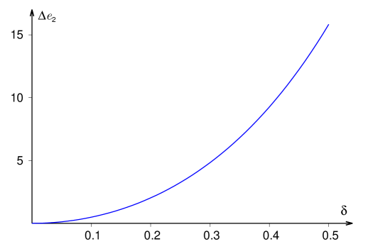
Figure 1: The difference $\Delta e_{2}\equiv e_{2}(\delta)-e_{2}(0)$, defined by (2.28), as a function of $\delta$ for $k_{1}=k_{2}=0$. Note that in this case $\Delta e_{2}=48.21714061416\ldots\times\delta^{2}+60.427986409885\ldots\times\,\delta^{4}+O(\delta^{6})$ as $\delta\to 0$.

3 Weak coupling expansion

We now consider a weak coupling expansion of the scaling function ${\mathfrak{F}}$. Since $g=\frac{\pi\delta}{1-\delta^{2}}=\pi\delta+O(\delta^{3})$, no needs to distinguish $\frac{g}{\pi}$ and $\delta$ within the first two perturbative orders. It is convenient to define the perturbative coefficients through the relation:

$${\mathfrak{F}}={\mathfrak{F}}_{0}+{\mathfrak{F}}_{1}\,\delta+{\mathfrak{F}}_{2}\,\delta^{2}+O(\delta^{3})\ .$$ (3.1)

Here ${\mathfrak{F}}_{0}(r,{\bf k})={\mathfrak{f}}(r,k_{+})+{\mathfrak{f}}(r,k_{-})$ with ${\mathfrak{f}}$ given by (2.21) (recall that $k_{\pm}=\frac{1}{2}\,(k_{1}\pm k_{2})$). The results obtained in the previous section allows one to predict the leading small-$R$ behavior of ${\mathfrak{F}}_{i}$. Generally speaking the coefficients in the power series (2.19) admit the Taylor expansion $e_{n}(\delta)=e_{n}(0)+\big{(}\frac{\partial e_{n}(0)}{\partial\delta}\big{)}_{p}\ \delta+\frac{1}{2}\ \big{(}\frac{\partial^{2}e_{n}(0)}{\partial\delta}\big{)}_{p}\ \delta^{2}+O(\delta^{3})$. In particular, as it follows from eq.(2.20),

$${\textstyle\big{(}\frac{\partial e_{1}(0)}{\partial\delta}\big{)}_{p}=0\ ,\ \ \ \ \big{(}\frac{\partial e_{1}(0)}{\partial\delta}\big{)}_{p}=\frac{1}{2}\ \psi^{\prime\prime\prime\prime}\big{(}{\textstyle\frac{1}{2}}\big{)}\ .}$$ (3.2)

Also, using the original integral representation (2.23) for $e_{2}(\delta)$, one can show that

$$\big{(}{\textstyle\frac{\partial e_{2}(0)}{\partial\delta}}\big{)}_{p}={\textstyle\frac{1}{4}}\,\big{(}\,\psi^{\prime}\big{(}{\textstyle\frac{1}{2}}+p_{1}+p_{2}\big{)}-\psi^{\prime}\big{(}{\textstyle\frac{1}{2}}-p_{1}-p_{2}\big{)}\big{)}\,\big{(}\psi^{\prime}\big{(}{\textstyle\frac{1}{2}}+p_{1}-p_{2}\big{)}-\psi^{\prime}\big{(}{\textstyle\frac{1}{2}}-p_{1}+p_{2}\big{)}\,\big{)}\,.$$ (3.3)

In the case $p_{1}=p_{2}=0$ the weak coupling expansion includes only even powers of $\delta$ (see Fig. 1) and

$${\textstyle\big{(}\frac{\partial^{2}e_{2}(0)}{\partial\delta^{2}}\big{)}_{p_{1}=p_{2}=0}=-{\textstyle\frac{1}{8}}\ \psi^{\prime\prime\prime\prime}\big{(}{\textstyle\frac{1}{2}}\big{)}\ .}$$ (3.4)

All of these can be used to study the short distance expansion of ${\mathfrak{F}}_{i}$ in eq.(3.1). In particular, it is possible to show that

$${\mathfrak{F}}_{1}(r,{\bf k})=-4\,{\mathfrak{q}}(r,k_{+})\,{\mathfrak{q}}(r,k_{-})\ ,$$ (3.5)

where

$${\mathfrak{q}}(r,k)=k+\big{(}\psi^{\prime}\big{(}{\textstyle\frac{1}{2}}+k\big{)}-\psi^{\prime}\big{(}{\textstyle\frac{1}{2}}-k\big{)}\big{)}\Big{(}{\frac{r}{4\pi}}\Big{)}^{2}-{\frac{1}{2}}\,\big{(}\psi^{\prime\prime\prime}\big{(}{\textstyle\frac{1}{2}}+k\big{)}-\psi^{\prime\prime\prime}\big{(}{\textstyle\frac{1}{2}}-k\big{)}\big{)}\,\Big{(}{\frac{r}{4\pi}}\Big{)}^{4}+O(r^{6})$$ (3.6)

and also

$${{\mathfrak{F}}_{2}=\frac{r^{2}}{4}\ \log\Big{(}\frac{r}{4\pi}\Big{)}+A\ \Big{(}{\frac{r}{4\pi}}\Big{)}^{2}-B\ \Big{(}{\frac{r}{4\pi}}\Big{)}^{4}+O(r^{6})\ ,}$$ (3.7)

where

$$A = -\psi^{\prime\prime}\big{(}{\textstyle\frac{1}{2}}\big{)}-\pi^{2}\ \Big{(}\psi\big{(}{\textstyle\frac{1}{2}}+k_{+}\big{)}+\psi\big{(}{\textstyle\frac{1}{2}}+k_{-}\big{)}+\psi\big{(}{\textstyle\frac{1}{2}}-k_{+}\big{)}+\psi\big{(}{\textstyle\frac{1}{2}}-k_{-}\big{)}\,\Big{)}$$

$$+ 2k_{+}^{2}\,\Big{(}\psi^{\prime\prime}\big{(}{\textstyle\frac{1}{2}}+k_{-}\big{)}+\psi^{\prime\prime}\big{(}{\textstyle\frac{1}{2}}-k_{-}\big{)}\,\Big{)}+2k^{2}_{-}\,\Big{(}\psi^{\prime\prime}\big{(}{\textstyle\frac{1}{2}}+k_{+}\big{)}+\psi^{\prime\prime}\big{(}{\textstyle\frac{1}{2}}-k_{+}\big{)}\,\Big{)}\ .$$

In the case $k_{1}=k_{2}=0$,

$$A|_{k_{1}=k_{2}=0}=-\psi^{\prime\prime}\big{(}{\textstyle\frac{1}{2}}\big{)}-4\pi^{2}\,\psi\big{(}{\textstyle\frac{1}{2}}\big{)}\ ,\ \ \ \ B|_{k_{1}=k_{2}=0}=-\psi^{\prime\prime\prime\prime}\big{(}{\textstyle\frac{1}{2}}\big{)}-4\pi^{2}\,\psi^{\prime\prime}\big{(}{\textstyle\frac{1}{2}}\big{)}\ .$$ (3.9)

For finite values of $r$ the perturbative coefficients ${\mathfrak{F}}_{i}$ can be calculated within the renormalized perturbation theory based on Lagrangian (1.2). Let ${\boldsymbol{S}}_{\sigma}({\bf x})\equiv\langle\,\psi_{\sigma}({\bf x})\otimes{\bar{\psi}}_{\sigma}({\bf 0})\,\rangle$ (${\bf x}=(x^{0},x^{1}),\,\sigma=\pm)$ be the fermionic Matsubara propagator with the temperature $1/R$ and chemical potential $2\pi{\rm i}k_{\sigma}/R$. It can be expressed in terms of the modified Bessel function of the second kind $K_{s}(z)=\frac{1}{2}\ \int_{-\infty}^{\infty}\mbox{d}\theta\ \mbox{e}^{s\theta-z\cosh(\theta)}$,

$${\boldsymbol{S}}_{\sigma}({\bf x})=\big{(}M-\gamma^{a}\partial_{a}\big{)}\ G_{\sigma}({\bf x})\ ,$$ (3.10)

where $\gamma^{a}$ are Euclidean $\gamma$-matrices, $\{\gamma^{a},\gamma^{b}\}=2\,\delta^{ab}$, and

$$G_{\sigma}({\bf x})=\frac{1}{2\pi}\ \sum_{n=-\infty}^{\infty}(-1)^{n}\ \mbox{e}^{2\pi{\rm i}nk_{\sigma}}\ K_{0}\big{(}|w-{\rm i}\,nr|\big{)}\ \ \ \ \ \ \ {\rm with}\ \ \ \ \ w=M\,(x^{0}+{\rm i}\,x^{1})\ .$$ (3.11)

At the first perturbative order one has (see Fig. 2)

$${\mathfrak{F}}_{1}=R^{2}\ {\rm Tr}\big{(}{\boldsymbol{S}}_{+}(0)\gamma_{a}\big{)}\,{\rm Tr}\big{(}{\boldsymbol{S}}_{-}(0)\gamma^{a}\big{)}=4R^{2}\ \langle\,\Psi^{\dagger}_{+}\,\Psi_{+}(0)\,\rangle\,\langle\,{\bar{\Psi}}^{\dagger}_{-}\,{\bar{\Psi}}_{-}(0)\,\rangle\ .$$ (3.12)

Here $\Psi_{\sigma}$ and ${\bar{\Psi}}_{\sigma}$ stand for the components of the Dirac bispinors $\psi_{\sigma}$ with the Lorentz spin $+\frac{1}{2}$ and $-\frac{1}{2}$, respectively.

\psfrag{a}{$-$}\psfrag{b}{$+$}\includegraphics[width=128.0374pt]{1pert.eps}

Figure 2: A diagrammatic representation of ${\mathfrak{F}}_{1}$ in eq. (3.1). The signs $\pm$ label the fermion “colors” $\psi_{\pm}$ propagating along the loops (see Lagrangian (1.2)).

In zero-temperature limit the Lorentz invariance is restored and hence $\langle\,{\bar{\Psi}}^{\dagger}_{\sigma}\,{\bar{\Psi}}_{\sigma}(0)\,\rangle=-\langle\,\Psi^{\dagger}_{\sigma}\,\Psi_{\sigma}(0)\,\rangle\to 0$. Introducing function ${\mathfrak{q}}$ through the relation

$$\langle\,{\bar{\Psi}}^{\dagger}_{\sigma}\,{\bar{\Psi}}_{\sigma}(0)\,\rangle=-\langle\,\Psi^{\dagger}_{\sigma}\,\Psi_{\sigma}(0)\,\rangle=\frac{1}{R}\ {\mathfrak{q}}(r,k_{\sigma})\ ,$$ (3.13)

one observes that ${\mathfrak{F}}_{1}$ takes the form (3.5). It is also easy to see that

$${\mathfrak{q}}=\frac{1}{4}\ \frac{\partial{\mathfrak{f}}}{\partial k}\ ,$$ (3.14)

where ${\mathfrak{f}}={\mathfrak{f}}(r,k)$ is given by (2.21). This is in a complete agreement with the short distance prediction (3.6).

The second-order diagrams are depicted in Fig. 3.

\psfrag{a}{$+$}\psfrag{b}{$-$}\psfrag{c}{$-\sigma$}\psfrag{d}{$\sigma$}\psfrag{G}{${\rm(I)}$}\psfrag{H}{${\rm(II)}$}\psfrag{W}{${\rm(III)}$}\includegraphics[width=455.24408pt]{2pert.eps}

Figure 3: The diagrams contributing to the second perturbative order. The contribution of the counterterm $\propto g_{1}$ in (1.2) is visualized by the type III diagrams (as $\nu=0$, there is no mass renormalization, i.e. $\delta M=0$).

The type I diagram gives the contribution

$${\mathfrak{F}}_{2}^{\rm(I)}=-\frac{\pi}{2}\ r^{2}\,\int_{D_{\epsilon}}\mbox{d}^{2}x\ {\rm Tr}\big{(}{\boldsymbol{S}}_{+}(-{\bf x})\,\gamma_{a}\,{\boldsymbol{S}}_{+}({\bf x})\,\gamma_{b}\big{)}\ {\rm Tr}\big{(}{\boldsymbol{S}}_{-}(-{\bf x})\,\gamma^{a}\,{\boldsymbol{S}}_{-}({\bf x})\,\gamma^{b}\big{)}\ .$$ (3.15)

Because of the UV divergence at ${\bf x}=0$, the integration domain $D_{\epsilon}$ here is chosen to be the cylinder (2.5) without an infinitesimal hole $|{\bf x}|<\epsilon$. One can show that, as $\epsilon$ tends to zero,

$${\mathfrak{F}}^{\rm(I)}_{2}=-\Big{(}\frac{R}{2\pi\epsilon}\Big{)}^{2}+\sum_{\sigma=\pm}\Big{(}{\mathfrak{t}}(r,k_{\sigma})-\frac{r}{2\pi}\,\log\big{(}{\textstyle\frac{M\epsilon}{2}}\,\mbox{e}^{\gamma_{E}-\frac{1}{2}}\big{)}\Big{)}^{2}+{\rm finite}\ ,$$ (3.16)

where

$${\mathfrak{t}}=-\pi\ \frac{\partial{\mathfrak{f}}}{\partial r}\ .$$ (3.17)

In fact, since $E_{\bf k}=R\,{\cal E}+\frac{\pi}{R}\,{\mathfrak{F}}$, the quadratic divergence $\propto 1/\epsilon^{2}$ should be relocated to the specific bulk energy. Generally speaking, the specific bulk energy has a form

$${\cal E}=w(g)\,\Lambda^{2}+\frac{M^{2}}{\pi}\,\cos^{2}\big{(}{\textstyle\frac{\pi\delta}{2}}\big{)}\ \log\big{(}M/\Lambda\big{)}+o(1)\ ,$$ (3.18)

where $\Lambda\gg M$ is some lattice energy scale and $w$ is some (nonuniversal) function of the coupling $g$. Notice that, in writing eq. (2.18), the quadratic divergence was omitted (as usual in QFT).

The type II diagrams from Fig. 3 leads to the UV finite integral over the whole cylinder $D$:

$${\mathfrak{F}}^{\rm(II)}_{2}=\frac{\pi}{2}\ r^{2}\,\int_{D}\mbox{d}^{2}x\ \sum_{\sigma=\pm}{\rm Tr}\big{(}{\boldsymbol{S}}_{\sigma}(0)\,\gamma_{a}\big{)}\,{\rm Tr}\big{(}{\boldsymbol{S}}_{-\sigma}(-{\bf x})\,\gamma^{a}\,{\boldsymbol{S}}_{-\sigma}({\bf x})\,\gamma^{b}\big{)}\,{\rm Tr}\big{(}{\boldsymbol{S}}_{\sigma}(0)\,\gamma_{b}\big{)}\ .$$ (3.19)

Finally, the counterterm $\propto g_{1}$ in (1.2) contributes through the type III diagrams, schematically visualized in Fig. 3. This can be written in the form $\frac{2g_{1}}{\pi}\ {\mathfrak{F}}^{\rm(III)}_{2}$ with

$${\mathfrak{F}}^{\rm(III)}_{2} = \frac{1}{4}\ R^{2}\ \sum_{\sigma=\pm}\Big{(}{\rm Tr}\big{(}{\boldsymbol{S}}_{\sigma}(0)\gamma^{a}\big{)}\,{\rm Tr}\big{(}{\boldsymbol{S}}_{\sigma}(0)\gamma_{a}\big{)}-{\rm Tr}\big{(}{\boldsymbol{S}}_{\sigma}(0)\gamma^{a}{\boldsymbol{S}}_{\sigma}(0)\gamma_{a}\big{)}\Big{)}$$ (3.20)

$$= R^{2}\sum_{\sigma=\pm}\big{(}\langle\,\Psi^{\dagger}_{\sigma}\,\Psi_{\sigma}(0)\,\rangle\langle\,{\bar{\Psi}}^{\dagger}_{\sigma}\,{\bar{\Psi}}_{\sigma}(0)\,\rangle-\langle\,{\bar{\Psi}}_{\sigma}\,\Psi^{\dagger}_{\sigma}(0)\,\rangle^{2}\big{)}\ .$$

Contrary to the one point functions (3.13), the condensate $\langle\,{\bar{\Psi}}_{\sigma}\,\Psi^{\dagger}_{\sigma}(0)\,\rangle$ diverges logarithmically:

$$\langle\,{\bar{\Psi}}_{\sigma}\,\Psi^{\dagger}_{\sigma}(0)\,\rangle=\langle\,{\Psi}_{\sigma}\,{\bar{\Psi}}^{\dagger}_{\sigma}(0)\,\rangle=\frac{1}{R}\ {\mathfrak{t}}(r,k_{\sigma})-\frac{M}{2\pi}\ \log\Big{(}\frac{M\epsilon}{2}\,\mbox{e}^{\gamma_{E}-\frac{1}{2}+C}\Big{)}\ ,$$ (3.21)

where $C$ is some constant. Since

$${\mathfrak{F}}^{\rm(I)}_{2}+{\mathfrak{F}}^{\rm(III)}_{2}+\Big{(}\frac{R}{2\pi\epsilon}\Big{)}^{2}=-\frac{r^{2}}{\pi^{2}}\ C\ \log(M\epsilon)+{\rm finite}\ ,$$ (3.22)

the UV divergence $\propto\log^{2}(\epsilon)$ is canceled from the sum of types I and III diagrams if we choose $g_{1}=\frac{g^{2}}{2\pi}+O(g^{3})$. As well as the quadratic divergence, the remaining logarithmic divergence should be relocated to the specific bulk energy. Expanding $\cos^{2}\big{(}{\textstyle\frac{\pi\delta}{2}}\big{)}$ in (3.18) one can find the value of the constant $C$:

$$C=\frac{\pi^{2}}{4}\ .$$ (3.23)

This way the second order correction takes the form

$${\mathfrak{F}}_{2}=\frac{r^{2}}{4\pi^{2}}\ {\cal C}_{2}+\lim_{\epsilon\to 0}\bigg{[}\,\sum_{\alpha={\rm I,II,III}}{\mathfrak{F}}^{(\alpha)}_{2}+\Big{(}\frac{R}{2\pi\epsilon}\Big{)}^{2}+\frac{r^{2}}{4}\ \log\Big{(}\frac{M\epsilon}{2}\,\mbox{e}^{\gamma_{\rm E}-\frac{1}{2}}\Big{)}\,\bigg{]}\ ,$$ (3.24)

where the finite constant should be adjusted to satisfy the normalization condition (2.10). It reads explicitly as

$${\cal C}_{2}=\frac{\pi^{4}}{8}-\frac{1}{2}-\frac{1}{4}\ \psi^{\prime\prime}\big{(}{\textstyle\frac{1}{2}}\big{)}\ .$$ (3.25)

Further calculations show that

$${\mathfrak{F}}_{2}(r,{\bf k}) = -\frac{1}{2}\,\ \big{(}1+c(2k_{1})+c(2k_{2})\big{)}\ \,r^{2}\,K_{0}(2r)$$

$$- \big{(}1-c(2k_{1})c(2k_{2})\big{)}\ r\,\int_{-\infty}^{\infty}\frac{\mbox{d}\nu}{\pi}\ \frac{\nu^{2}\,K_{{\rm i}\nu}(r)K_{1+{\rm i}\nu}(r)}{\sinh^{2}(\frac{\pi\nu}{2})}+o\big{(}\mbox{e}^{-2r}\big{)}\ .$$

Here the shortcut notation $c(k)=\cos(\pi k)$ is used and $K_{s}(z)$ denotes the modified Bessel function of the second kind:

$$K_{s}(z)=\frac{1}{2}\ \int_{-\infty}^{\infty}\mbox{d}\theta\ \mbox{e}^{s\theta-z\cosh(\theta)}\ .$$ (3.27)

Also in eq. (3) and bellow, the symbol $o\big{(}\mbox{e}^{-2r}\big{)}$ denotes a remaining term that decays faster than $r^{-N}\ \mbox{e}^{-2r}$ for any positive $N$ as $r\to+\infty$. Notice that the normalization condition ${\mathfrak{F}}_{2}=o\big{(}\mbox{e}^{-r}\big{)}$ implies an absence of the finite renormalization of the fermion mass. It can be used for fixing the constant $C$ in (3.21) and hence avoid any reference to the exact relation (3.18). For $k_{1}=k_{2}=0$, the result of perturbative calculation is presented in Fig. 4.

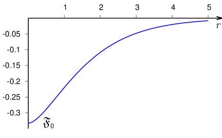
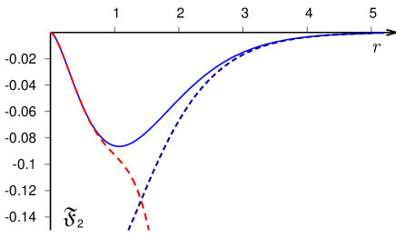
Figure 4: The perturbative coefficient ${\mathfrak{F}}_{i}$ (3.1) for $k_{1}=k_{2}=0$ $({\mathfrak{F}}_{1}=0$ in this case). The left panel shows ${\mathfrak{F}}_{0}=-\frac{2r}{\pi^{2}}\ \int_{-\infty}^{\infty}\mbox{d}\theta\,\cosh(\theta)\,\log\big{(}1+\mbox{e}^{-r\cosh(\theta)}\big{)}$. At the right panel ${\mathfrak{F}}_{2}$ is compared against its large-$r$ asymptotic ${\mathfrak{F}}_{2}=-\frac{3}{2}\,r^{2}\,K_{0}(2r)+o(\mbox{e}^{-2r})$ (blue dashed line) and the small-$r$ asymptotic ${\mathfrak{F}}_{2}=\frac{r^{2}}{4}\,\log\big{(}\frac{r}{4\pi}\big{)}+A\,\big{(}\frac{r}{4\pi}\big{)}^{2}-B\,\big{(}\frac{r}{4\pi}\big{)}^{4}+O(r^{6})$ (red dashed line). The numerical coefficients $A$ and $B$ are given by eq.(3.9).

Using eqs. (3.5) and (3.14) it is easy to show that

$${\mathfrak{F}}_{1}(r,{\bf k})=\frac{2}{\pi^{2}}\ \big{(}c(2k_{1})-c(2k_{2})\big{)}\ r^{2}\,K_{1}^{2}(r)+o\big{(}\mbox{e}^{-2r}\big{)}\ .$$ (3.28)

Thus, at least at the first-two perturbative orders, the leading large-$r$ behavior of the scaling function ${\mathfrak{F}}$ is defined by ${\mathfrak{F}}_{0}$ only and therefore

$${\mathfrak{F}}(r,{\bf k})=-\frac{4}{\pi^{2}}\ c(k_{1})\,c(k_{2})\ r\,K_{1}(r)+o(\mbox{e}^{-r})\ .$$ (3.29)

This can be understood as follows. The leading large-$R$ behavior comes from the virtual fermions trajectories winding once around the Matsubara circle. Such trajectories should be counted with the phase factor $\mbox{e}^{{\rm i}\pi(\sigma_{1}k_{1}+\sigma_{2}k_{2})}$ and, therefore, the summation over four possible sign combinations with $\sigma_{1,2}=\pm 1$ gives rise eq.(3.29). Thus we may expect that the asymptotic formula (3.29) holds true as the mass of the first bound state $M_{1}=2M\,\cos(\frac{\pi\delta}{2})$ is greater than $M$, i.e., for $\delta\in[0,\frac{2}{3})$.

Before concluding this section let us make a few remarks about the (non-integrable) case with a non-zero value of $\nu$. Instead of adjusting the counterterm coupling $g_{1}$, the logarithmic divergences can be absorbed by the mass counterterm with $\delta M=\nu\ \log(M/\Lambda_{\rm UV})$, where $\nu=\frac{g^{2}}{\pi^{2}}-\frac{2g_{1}}{\pi}$ and $\Lambda_{\rm UV}=\frac{2}{\epsilon}\ \exp(\frac{1}{2}-\gamma_{\rm E}-\frac{\pi^{2}}{4})$. (This is an infinitesimal version of eq. (1.3) where $M_{0}=M+\delta M$.) As it was mentioned in the introduction, the exponent $\nu$ and the four-fermion coupling $g$ can be thought of as independent parameters for the family of BL models. Using eq. (3.20), it is easy to see that

$$\frac{\partial{\mathfrak{F}}}{\partial\nu}\Big{|}_{\nu=0}=\sum_{\sigma=\pm}\big{(}{\mathfrak{q}}^{2}(r,k_{\sigma})+{\mathfrak{t}}^{2}(r,k_{\sigma})\big{)}+O(g)\ .$$ (3.30)

Finally we note that for $\nu\not=0$, (an universal part of) the specific bulk energy has a valid Laurent expansion of the form

$${\cal E}(g,\nu)=M^{2}\,\Big{(}\,h_{-1}(g)\,\nu^{-1}+\sum_{n=0}^{\infty}h_{n}(g)\ \nu^{n}\,\Big{)}\ ,$$ (3.31)

where $h_{n}(g)$ admit power series expansions in $g^{2}$.

4 Exact formula for ${\mathfrak{F}}(r,{\bf k})$

The BL model with non-vanishing $\nu=\frac{1}{2}\,(a_{1}+a_{2}-2)$ can be thought as a sort of analytical regularization of the model with $\nu=0$ – the integrals appearing in the conformal perturbation theory converge for negative values of $\nu$, but become singular at $\nu\to 0^{-}$. A brief inspection of eq. (2.8) shows that a simple pole $\frac{1}{\nu}$ replaces the logarithmic divergence $2\,\log(\epsilon\mu)+const$ in (2.13) which occurs when the integral is regularized by excluding a neighborhood of the singular point from the integration domain. The BL with non-vanishing $\nu$ is a well defined QFT and it is interesting in itself in a context of applications in condensed matter physics [17]. However, as it was already mentioned in the introduction, the “$\nu$-deformation” spoils the integrability. Remarkably that there exists an integrable deformation of the BL model with $\nu=0$. The corresponding model was introduced by Fateev in the works [18, 6] and it will be referred to bellow as the Fateev model.

Contrary to the BL model, the Fateev (F) model involves three Bose fields governed by the Lagrangian

$${\tilde{\cal L}}_{\rm F} = \frac{1}{16\pi}\ \sum_{i=1}^{3}\big{(}\,(\partial_{0}\varphi_{i})^{2}-(\partial_{1}\varphi_{i})^{2}\,\big{)}$$

$$+ 2\mu\ \big{(}\,\mbox{e}^{{\rm i}\,\alpha_{3}\varphi_{3}}\ \cos(\alpha_{1}\varphi_{1}+\alpha_{2}\varphi_{2})+\mbox{e}^{-{\rm i}\alpha_{3}\varphi_{3}}\ \cos(\alpha_{1}\varphi_{1}-\alpha_{2}\varphi_{2})\,\big{)}\,.$$

Here $\alpha_{i}=\frac{1}{2}\sqrt{a_{i}}$ and the coupling constants $a_{i}$ satisfy a single constraint

$$a_{1}+a_{2}+a_{3}=2\ ,$$ (4.2)

which implies that the parameter $\mu$ has a dimension of mass. As $\alpha_{3}\to 0$, the field $\varphi_{3}$ decouples in (4) and the interacting part coincides with the bosonic version of the BL Lagrangian (1.4) with $a_{1}+a_{2}=2$. In fact, this observation requires a more careful assessment. Performing the limit $\alpha_{3}\to 0$, one should expand the exponentials $\mbox{e}^{\pm{\rm i}\,\alpha_{3}\varphi_{3}}$ in (4) to the terms $\propto a_{3}=4\alpha^{2}_{3}$. The mass of the decoupled field is given by the relation $m^{2}=8\pi\mu a_{3}\,\langle\,\cos(\alpha_{1}\varphi_{1})\cos(\alpha_{2}\varphi_{2})\,\rangle$, where the vacuum expectation value is taken for the BL model with $\nu=0$. This expectation value is simply related to the corresponding specific bulk energy, $\langle\,\cos(\alpha_{1}\varphi_{1})\cos(\alpha_{2}\varphi_{2})\,\rangle=-\frac{1}{4}\ \frac{\partial{\cal E}}{\partial\mu}$, and hence

$$m^{2}=-2\pi\mu\,\lim_{a_{3}\to 0}\,\Big{(}a_{3}\ \frac{\partial{\cal E}}{\partial\mu}\,\Big{)}\ .$$ (4.3)

Eq. (2.18) shows that ${\cal E}=4\pi\mu^{2}\,\log(\mu\epsilon)+\ldots$ and, as has been argued above, should be replaced by ${\cal E}=\frac{4\pi\mu^{2}}{a_{1}+a_{2}-2}+\ldots$ within the analytical regularization. This, combined with (4.3) and the constraint $a_{3}=2-a_{1}-a_{2}$, means that the field $\varphi_{3}$ has the mass $m=4\pi\mu$ in the decoupling limit. Taking into account $M-\mu$ relation (2.17), one finally obtains

$$m=2M\,\cos\big{(}{\textstyle\frac{\pi\delta}{2}}\big{)}\ ,$$ (4.4)

where we use $\delta=1-a_{1}=a_{2}-1$.

One of Fateev’s important results concerning the theory (4) is an elegant analytical expression for the specific bulk energy [6]:

$${\cal E}_{\rm F}=-\pi\mu^{2}\ \prod_{i=1}^{3}\frac{\Gamma(\frac{a_{i}}{2})}{\Gamma(1-\frac{a_{i}}{2})}\ .$$ (4.5)

The linear constraint imposed on parameters $a_{i}$, can be resolved by setting $a_{1}=1-\delta-\frac{a_{3}}{2}$ and $a_{2}=1+\delta-\frac{a_{3}}{2}$, and, therefore, as $a_{3}\to 0$ one has

$${\cal E}_{\rm F}=\pi\mu^{2}\,\Big{(}-\frac{2}{a_{3}}-4\log 2+\psi\big{(}{\textstyle\frac{1+\delta}{2}}\big{)}+\psi\big{(}{\textstyle\frac{1-\delta}{2}}\big{)}-2\psi\big{(}{\textstyle\frac{1}{2}}\big{)}+o(1)\,\Big{)}\ .$$ (4.6)

Keeping in mind that $\frac{1}{a_{3}}$ can be substituted by $(-\log(\mu\epsilon))$ one find the relation

$${\cal E}_{\rm F}\to{\cal E}+const\ m^{2}\ \ \ \ {\rm as}\ \ \ \ a_{3}\to 0\ ,$$ (4.7)

where ${\cal E}$ is the specific bulk energy for the BL model (2.18), whereas the term $\propto m^{2}$ is a contribution of the free massive field. Notice that $const$ does not depend on the coupling $\delta$, and it can be always set to zero.

We can consider now the Fateev model in finite volume with the periodic boundary conditions $\varphi_{i}(x^{0},x^{1}+R)=\varphi_{i}(x^{0},x^{1})$ imposed on all three fields $\varphi_{i}$. Similar to the definition (2.9) for the BL model, let us introduce ${\mathfrak{F}}_{\rm F}=R\,({E}_{\bf k}-R{\cal E}_{\rm F})/\pi$. Then the above consideration suggests that

$$\lim_{a_{3}\to 0^{-}}{\mathfrak{F}}_{\rm F}={\mathfrak{F}}(r,{\bf k})+{\mathfrak{f}}_{\rm B}\big{(}2rc\big{(}{\textstyle\frac{\delta}{2}}\big{)}\big{)}\ ,$$ (4.8)

where the second term in the r.h.s. with

$${\mathfrak{f}}_{\rm B}(\beta)=\frac{\beta}{2\pi^{2}}\ \int_{-\infty}^{\infty}\mbox{d}\theta\ \cosh(\theta)\ \log\big{(}1-\mbox{e}^{-\beta\cosh(\theta)}\big{)}\ ,$$ (4.9)

corresponds to a contribution of the free boson of mass $2Mc\big{(}{\textstyle\frac{\delta}{2}}\big{)}$ with $c(x)\equiv\cos(\pi x)$. Notice that the limit in (4.8) should be taken from negative values of $a_{3}$, so that the Lagrangian (4) is real. For $a_{i}>0\ (i=1,2,3)$ the Lagrangian is complex, but the QFT is still well defined. In this case the potential term in (4) is periodic w.r.t. all fields $\varphi_{i}$ and the space of states splits on the orthogonal subspaces characterized by a triple of quasimomenta ${\bf k}=(k_{1},k_{2},k_{3})$. For $a_{3}<0$ different sectors of the theory are labeled by a pair of quasimomenta, similar to the case of the BL model, so that eq. (4.8) can be understood literally as a relation between the vacuum energies in the Fateev and BL models characterized by the same ${\bf k}=(k_{1},k_{2})$.

A major advantage of the case with all positive $a_{i}$ is that the general structure of the small-$R$ expansion in this regime is considerably simple compared to the case $a_{3}<0$. For $a_{i}>0$ the potential term in the Lagrangian (4) is a uniformly bounded perturbation for any finite value of the dimensionless product $\mu R$. Therefore the conformal perturbation theory yields an expansion of the form

$$\frac{R}{\pi}\,E_{\rm F}=-\sum_{n=0}^{\infty}e^{(\rm F)}_{2n}\ (\mu R)^{4n}\ \ \ \ \ \ \ (a_{i}>0)\ .$$ (4.10)

Here $e^{(\rm F)}_{0}=\frac{1}{6}\sum_{i=1}^{3}\big{(}1-6\,a_{i}\,k_{i}^{2}\,\big{)}$, whereas the coefficients $e^{(\rm F)}_{2n}$ for $n\geq 1$ are expressed in terms of convergent 2D Coulomb-type integrals, for example

$$e^{(\rm F)}_{2} = 2\int\prod_{i=1}^{3}\frac{\mbox{d}^{2}z_{i}}{2\pi}\ |z_{1}|^{-1+2p_{1}+2p_{2}+2p_{3}}\ |z_{2}|^{-1-2p_{1}+2p_{2}-2p_{3}}\ |z_{3}|^{-1-2p_{1}-2p_{2}+2p_{3}}\$$

$$\times \big{|}(z_{1}-1)(z_{2}-z_{3})\big{|}^{2a_{1}-2}\ \big{|}(z_{1}-z_{2})(z_{3}-1)\big{|}^{2a_{2}-2}\ \big{|}(z_{1}-z_{3})(z_{2}-1)\big{|}^{2a_{3}-2}\ ,$$

where $p_{i}=\frac{1}{2}\,a_{i}k_{i}$. Notice that the integral diverges at $a_{3}\to 0^{+}$ and formula  (2.23) for the asymptotic coefficient $e_{2}(\delta)$ in the BL model is a regularized version of $e^{(\rm F)}_{2}$ with $p_{3}=0$. Similarly to the expression for $e_{2}(\delta)$, eq. (4) can be brought to the form

$$e^{(\rm F)}_{2}=\frac{1}{4\pi}\ \int\mbox{d}^{2}\zeta\ |\zeta|^{2a_{1}-4}|1-\zeta|^{2a_{2}-4}\ \big{(}\tau_{p_{1}p_{2}p_{3}}(\zeta)\big{)}^{2}\ ,$$ (4.12)

where

$$\tau_{p_{1}p_{2}p_{3}}(\zeta)=-\frac{1}{2p_{1}}\sum_{\sigma=\pm}\sigma\,\sqrt{\Omega(\sigma p_{1},p_{2}+p_{3})\Omega(\sigma p_{1},p_{2}-p_{3})}\ \ \big{|}\chi_{\sigma p_{1},p_{2},p_{3}}(\zeta)\big{|}^{2}$$ (4.13)

and

$$\chi_{p_{1}p_{2}p_{3}}(\zeta)=\zeta^{\frac{1}{2}+p_{1}}(1-\zeta)^{\frac{1}{2}+p_{2}}\ \,{}_{2}F_{1}\big{(}{\textstyle\frac{1}{2}}+p_{1}+p_{2}+p_{3},{\textstyle\frac{1}{2}}+p_{1}+p_{2}-p_{3},1+2p_{1};\zeta\big{)}\ .$$ (4.14)

The derivation follows the same steps outlined in Sec. 2; Fist of all, one should substitute the integration variables $z_{2}$ by $\zeta=\frac{(1-z_{1})(z_{2}-z_{3})}{(1-z_{2})(z_{1}-z_{3})}$. Then the integral over $z_{1}$ is performed using the identity (2.24) where $p_{1}$ is substituted by $p_{1}+p_{3}$. Finally one should use the identity generalizing (2.27):

$$\big{(}\tau_{p_{1}p_{2}p_{3}}(\zeta)\big{)}^{2}=|\zeta|^{2}\ \int\frac{\mbox{d}^{2}z}{\pi|z|^{2}}\ \Big{|}\frac{1-\zeta z}{z(z-\zeta)}\Big{|}^{2p_{1}+2p_{3}}\ |z|^{4p_{3}}\ \frac{\tau_{p_{1}+p_{3},p_{2},0}\big{(}X(z)\big{)}}{|X(z)|}\ ,$$ (4.15)

where $X(z)=\frac{(\zeta-z)(1-\zeta z)}{\zeta(1-z)^{2}}$. An important observation is that $\tau_{p_{1}p_{2}p_{3}}(\zeta)$, considered as a function on the Riemann sphere, is regular except for three points $\zeta=0,\,1,\infty$ and

$$\eta_{\rm L}=-\log\tau_{p_{1}p_{2}p_{3}}(\zeta)$$ (4.16)

is a real solution of the Liouville equation

$$\partial_{\zeta}\partial_{\bar{\zeta}}\eta_{\rm L}-\mbox{e}^{2\eta_{\rm L}}=0$$ (4.17)

for $|p_{i}|<\frac{1}{2},\ \sum_{i}|p_{i}|<\frac{1}{2}$ (for details, see e.g. ref. [19]). Notice that $\tau_{p_{1}p_{2}p_{3}}(\zeta)=\tau_{p_{1}p_{2}p_{3}}(1-\zeta)=|\zeta|^{2}\,\tau_{p_{3}p_{2}p_{1}}(\zeta^{-1})$ and therefore $\eta_{\rm L}$ satisfy the following asymptotic conditions at the punctures:

$$\eta_{\rm L}\to\begin{cases}(2|p_{1}|-1)\,\log|\zeta|+O(1)\ \ \ &{\rm as}\ \ \ \zeta\to 0\\ (2|p_{2}|-1)\,\log|\zeta-1|+O(1)\ \ \ &{\rm as}\ \ \ \zeta\to 1\\ (2|p_{3}|+1)\,\log|1/\zeta|+O(1)\ \ \ &{\rm as}\ \ \ \zeta\to\infty\end{cases}\ .$$ (4.18)

This way the result of conformal perturbation theory can be expressed in terms of solution of the Liouville equation on the three-punctured sphere ${\mathbb{S}}^{2}/\{0,\,1,\infty\}$:

$$\frac{R}{\pi}\ E_{\rm F}=-\frac{1}{6}\ \sum_{i=1}^{3}\Big{(}1-\frac{24}{a_{i}}\ p_{i}^{2}\,\Big{)}-\frac{1}{4\pi}\ \int\mbox{d}^{2}\zeta\ |P(\zeta)|^{2}\ \mbox{e}^{-2\eta_{\rm L}}+O(\rho^{8})\ \ \ \ (a_{i}>0)\ ,$$ (4.19)

where $\rho=\frac{1}{2}\ \mu R$ and

$$P(\zeta)=\rho^{2}\ \zeta^{a_{1}-2}(1-\zeta)^{a_{2}-2}\ .$$ (4.20)

In ref. [13] it was conjectured that

$$\frac{R}{\pi}\ E_{\rm F}=-\frac{1}{6}\ \sum_{i=1}^{3}\Big{(}1-\frac{24}{a_{i}}\ p_{i}^{2}\,\Big{)}-\frac{1}{4\pi}\ \int\mbox{d}^{2}\zeta\ |P(\zeta)|^{2}\ \mbox{e}^{-2\eta}\ \ \ \ \ \ \ (a_{i}>0)\ ,$$ (4.21)

where $\eta$ is a real solution of the so-called modified sinh-Gordon equation

$$\partial_{\zeta}\partial_{\bar{\zeta}}\eta-\mbox{e}^{2\eta}+|P(\zeta)|^{2}\ \mbox{e}^{-2\eta}=0\ ,$$ (4.22)

satisfying the the same asymptotic conditions as (4.18) (i.e., $\eta_{\rm L}$ should be substituted by $\eta$ in (4.18)). The last term in (4.22) $\propto\rho^{4}$ and can be treated perturbatively for $|p_{i}|<\frac{a_{i}}{4}$. Therefore the small-$R$ behavior (4.19) follows immediately from the exact formula (4.21). One can show that the leading large-$R$ asymptotic of (4.21) correctly reproduces the specific bulk energy (4.5) (see ref.[13] for details). Additional arguments in support of eq. (4.21) were presented in the work [14].

Eq. (4.21) can be transformed to a formula for the scaling function ${\mathfrak{F}}_{\rm F}\equiv R\,(E_{\rm F}-R{\cal E}_{\rm F})/\pi$. For this purpose, one should consider the Schwarz-Christoffel mapping

$$w(\zeta)=\int\mbox{d}\zeta\ \sqrt{P(\zeta)}\ ,$$ (4.23)

which maps the upper half plane $\Im m(\zeta)\geq 0$ to the triangle $(w_{1},\,w_{2},\,w_{3})$ in the complex $w$-plane (see Fig. 5).

\psfrag{a}{$\pi a_{1}$}\psfrag{b}{$\pi a_{2}$}\psfrag{c}{$\frac{\pi a_{1}}{2}$}\psfrag{d}{$\frac{\pi a_{2}}{2}$}\psfrag{e}{$\frac{\pi a_{3}}{2}$}\psfrag{w1}{$w_{1}$}\psfrag{w2}{$w_{2}$}\psfrag{w3}{$w_{3}$}\psfrag{bw3}{${\bar{w}}_{3}$}\includegraphics[width=128.0374pt]{triangle1.eps}

Figure 5: Triangle $(w_{1},w_{2},w_{3})$ is a $w$-image of the upper half plane $\Im m(\zeta)>0$ under the Schwarz-Christoffel mapping (4.23) with $a_{i}>0$. The point ${\bar{w}}_{3}$ is a reflection of $w_{3}$ w.r.t. the straight line $(w_{1},w_{2})$. The domain ${\mathbb{D}}_{\rm F}^{(+)}$ is obtained from the 4-polygon $(w_{1},w_{3},w_{2},{\bar{w}}_{3})$ by the identification of the sides $[w_{1},w_{3}]\sim[w_{1},{\bar{w}}_{3}]$ and $[w_{2},w_{3}]\sim[w_{2},{\bar{w}}_{3}]$.

The lower half plane $\Im m(\zeta)\leq 0$ is mapped into the congruent triangle $(w_{1},w_{2},{\bar{w}}_{3})$. It is straightforward to show that the real function ${\hat{\eta}}={\eta}-{\textstyle\frac{1}{4}}\ \log(P{\bar{P}})$ is a solution of the sinh-Gordon equation

$$\partial_{w}\partial_{\bar{w}}{\hat{\eta}}-\mbox{e}^{2{\hat{\eta}}}+\mbox{e}^{-2{\hat{\eta}}}=0$$ (4.24)

in the open domain ${\mathbb{D}}_{\rm F}^{(+)}$, which is obtained by gluing together the triangles along their sides, as it shown in Fig. 5. At the singular points $w=w_{i}\ (i=1,2,3)$ the solution has the following asymptotic behavior:

$${\hat{\eta}}=(2|k_{i}|-1)\ \log|w-w_{i}|+O(1)\ \ \ \ \ \ \ \ {\rm as}\ \ \ \ \ w\to w_{i}\ .$$ (4.25)

In ref. [13] it was shown that formula (4.21) implies the relation

$${\mathfrak{F}}_{\rm F}=-{\frac{8}{\pi}}\ \int_{{\mathbb{D}}_{\rm F}^{(+)}}\mbox{d}^{2}w\ \sinh^{2}({\hat{\eta}})+\sum_{i=1}^{3}a_{i}\,\big{(}|k_{i}|-{\textstyle\frac{1}{2}}\big{)}^{2}\ \ \ \ \ \ (a_{i}>0)\ .$$ (4.26)

Then, in the consequent paper [15], it was argued that (4.26), with some minor modifications, also applies to the case $a_{1,2}>0$, $a_{3}<0$. Namely,

$${\mathfrak{F}}_{\rm F}=-{\frac{8}{\pi}}\ \int_{{\mathbb{D}}^{(-)}_{\rm F}}\mbox{d}^{2}w\ \sinh^{2}({\hat{\eta}})+\sum_{i=1}^{2}a_{i}\,\big{(}|k_{i}|-{\textstyle\frac{1}{2}}\big{)}^{2}\ \ \ \ \ \ (a_{1},a_{2}>0,\ a_{3}<0)\ ,$$ (4.27)

where now ${\hat{\eta}}$ is a solution of the sinh-Gordon equation (4.24) in the domain shown in Fig. 6, satisfying the asymptotic conditions (4.25) at the vertices $w_{1}$ and $w_{2}$, and

$${\hat{\eta}}\to 0\ \ \ \ \ {\rm as}\ \ \ \ |w|\to\infty\ .$$ (4.28)

\psfrag{a}{$\pi a_{1}$}\psfrag{b}{$\pi a_{2}$}\psfrag{c}{$\frac{\pi a_{1}}{2}$}\psfrag{d}{$\frac{\pi a_{2}}{2}$}\psfrag{e}{$\frac{\pi a_{3}}{2}$}\psfrag{w1}{$w_{1}$}\psfrag{w2}{$w_{2}$}\psfrag{w3}{$w_{3}$}\psfrag{bw3}{${\bar{w}}_{3}$}\includegraphics[width=113.81102pt]{domain1.eps}

Figure 6: Domain ${\mathbb{D}}_{\rm F}^{(-)}$ – the image of the thrice-punctured sphere for the case of Schwarz-Christoffel mapping (4.23) with $a_{1,2}>0$, $a_{3}<0$.

As $a_{3}\to 0^{-}$, the domain ${\mathbb{D}}_{\rm F}^{(-)}$ tends to the region ${\mathbb{D}}_{\rm BL}$ shown in Fig. 7.

\psfrag{a}{$\pi a_{1}$}\psfrag{b}{$\pi a_{2}$}\psfrag{c}{$r/4$}\psfrag{w1}{$w_{1}$}\psfrag{w2}{$w_{2}$}\psfrag{w}{$w$}\includegraphics[width=128.0374pt]{domain.eps}

Figure 7: Domain ${\mathbb{D}}_{\rm BL}$ – the image of the thrice-punctured sphere for the case of Schwarz-Christoffel mapping (4.23) with $a_{1}+a_{2}=2$. The overall size of ${\mathbb{D}}_{\rm BL}$ is controlled by a length of the segment $(w_{1},w_{2})$, which coincides with $r/4$

With the relation (4.8), this leads to the following exact formula for the scaling function ${\mathfrak{F}}(r,{\bf k})$ in the BL model,

$${\mathfrak{F}}(r,{\bf k})=-{\mathfrak{f}}_{\rm B}\big{(}2rc\big{(}{\textstyle\frac{\delta}{2}}\big{)}\big{)}-{\frac{8}{\pi}}\ \int_{{\mathbb{D}}_{\rm BL}}\mbox{d}^{2}w\ \sinh^{2}({\hat{\eta}})+\sum_{i=1}^{2}a_{i}\,\big{(}|k_{i}|-{\textstyle\frac{1}{2}}\big{)}^{2}\ .$$ (4.29)

As we shall see below this formula is in a perfect agreement with all perturbation theory calculations, considered in Sec. 2 and Sec. 3 of this paper, as well as with all other known results on the BL model, including the Bethe ansatz results of [3, 12].

The sinh-Gordon equation (4.24) is a classical integrable equation which can be treated by the inverse scattering transform method. Thus the relation (4.29) allows one to apply this powerful method to the problem of determining the vacuum energies. The working is very similar to that for the Fateev model, considered in [14], where all $a_{1},a_{2},a_{3}>0$, though contains a few original details. We postpone these derivations to our future publication [40] but present the final result here. The scaling function (4.29) is expressed through the solution of a system of two Non-Linear Integral Equations (NLIE):

$$\varepsilon_{\sigma}(\theta)=r\,\sinh(\theta-{\rm i}\chi_{\sigma})-2\pi k_{\sigma}+\sum_{\sigma^{\prime}=\pm}\int_{-\infty}^{\infty}\frac{\mbox{d}\theta^{\prime}}{\pi}\,{G}_{\sigma\sigma^{\prime}}(\theta-\theta^{\prime})\ \Im m\Big{[}\log\big{(}1+e^{-{\rm i}\varepsilon_{\sigma^{\prime}}(\theta^{\prime}-{\rm i}0)}\big{)}\Big{]}.$$ (4.30)

Here $\sigma=\pm$, $(\chi_{+},\chi_{-})=(0,\,\pi a_{1}/2)$ and the kernels are given by the relations

$$G_{\pm\pm}(\theta)=G_{a_{1}}(\theta)+G_{a_{2}}(\theta)\ ,\ \ \ \ \ \ {G}_{\pm\mp}(\theta)={\hat{G}}_{a_{1}}(\theta)-{\hat{G}}_{a_{2}}(\theta)\ .$$ (4.31)

with

$$G_{a}(\theta) = \int_{-\infty}^{\infty}\mbox{d}\nu\ \frac{\mbox{e}^{{\rm i}\nu\theta}\,\sinh(\frac{\pi\nu}{2}(1-a))}{2\cosh(\frac{\pi\nu}{2})\sinh(\frac{\pi\nu a}{2})}$$ (4.32)

$${\hat{G}}_{a}(\theta) = \int_{-\infty}^{\infty}\mbox{d}\nu\ \frac{\mbox{e}^{{\rm i}\nu\theta}\,\sinh(\frac{\pi\nu}{2})}{2\cosh(\frac{\pi\nu}{2})\sinh(\frac{\pi\nu a}{2})}\ .$$

Once the numerical data for $\varepsilon_{\pm}(\theta)$ are available, ${\mathfrak{F}}(r,{\bf k})$ (4.29) can be computed by means of the relation

$${\mathfrak{F}}(r,{\bf k})=\pm\frac{r}{\pi}\ \Im m\Big{[}L_{+}(\pm{\rm i})+\mbox{e}^{\mp\frac{{\rm i}\pi}{2}a_{1}}\,L_{-}(\pm{\rm i})\,\Big{]}\ ,$$ (4.33)

where

$$L_{\sigma}(\nu)=\int_{-\infty}^{\infty}\frac{\mbox{d}\theta}{\pi}\ \mbox{e}^{-{\rm i}\nu\theta}\,\log\big{(}1+e^{-{\rm i}\varepsilon_{\sigma}(\theta-{\rm i}0)}\big{)}\ .$$ (4.34)

Notice that (4.33) is valid for both choices of the sign $\pm$.

Eq.(4.33) can be compared against the predictions of renormalized perturbation theory in several ways. First, note that the integral equation (4.30) have a smooth limit for $\delta\to 0$ (its kernel vanishes linearly in $\delta$). Using this property we have verified that the function ${\mathfrak{F}}_{2}$ in eq. (3.1), extracted from the numerical solution of (4.30)-(4.34) for $k_{1}=k_{2}=0$ and $0.1\leq r\leq 5$, within nine significant digits coincides with the result of the perturbative calculations, shown with the solid line in the right panel of Fig. 4. Second, one can show that the exact formula (4.33) implies the following large-$R$ asymptotics

$${\mathfrak{F}}(r,{\bf k})={\mathfrak{F}}_{0}(r,{\bf k})+{\mathfrak{f}}_{\rm B}(2r)-{\mathfrak{f}}_{\rm B}\big{(}2rc\big{(}{\textstyle\frac{\delta}{2}}\big{)}\big{)}+\frac{16r}{\pi^{2}}\ \sum_{i=1}^{2}\int_{-\infty}^{\infty}\frac{\mbox{d}\nu}{2\pi}\$$ (4.35)

$$\times\ \Big{(}c^{2}(k_{1})\,c^{2}(k_{2})-c^{2}(k_{3-i})\,\cosh^{2}\big{(}{\textstyle\frac{\pi\nu}{2}}\big{)}\Big{)}\ K_{{\rm i}\nu}(r)K_{1-{\rm i}\nu}(r)\ \frac{\sinh(\frac{\pi\nu}{2}(1-a_{i}))}{\cosh(\frac{\pi\nu}{2})\sinh(\frac{\pi\nu}{2}a_{i})}+o\big{(}\mbox{e}^{-2r}\big{)}\ ,$$

where $k_{1}=k_{+}+k_{-},\,k_{2}=k_{+}-k_{-}$ and $c(x)\equiv\cos(\pi x)$. Expanding this relation to the second order in $\delta=1-a_{1}=a_{2}-1$, one finds that the result is consistent with eqs. (3.1), (3.28) and (3) from Sec. 3. Third, the numerical values for ${\mathfrak{F}}(r,{\bf k})$ obtained from (4.33) and presented in Fig. 8 and Tab. 1 on page 1, show an excellent agreement with the large-$R$ asymptotic formula (4.35) and also with the predictions of the conformal perturbation theory, given by (2.19), (2.20) and (2.28).

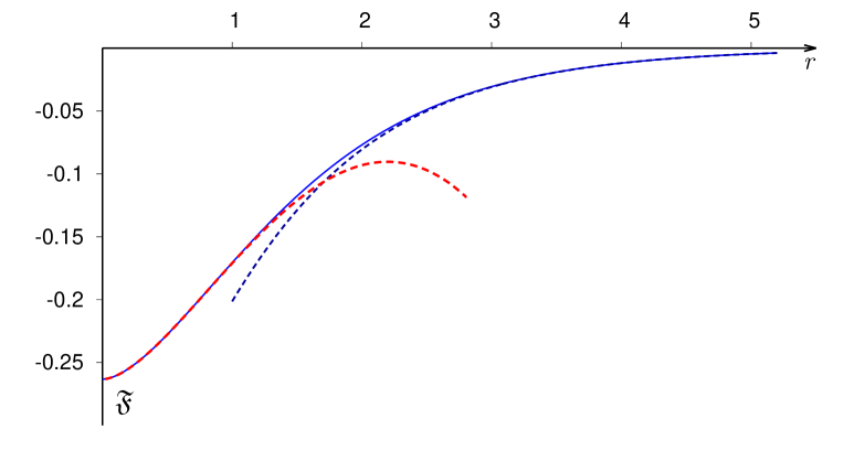
Figure 8: The scaling function ${\mathfrak{F}}(r,{\bf k})$ as a function of $r=MR$ for $\delta=\frac{17}{47}=0.36\ldots,\ k_{1}=\frac{47}{150},\ k_{2}=\frac{47}{640}$. The solid line was obtained from numerical integration of (4.30), (4.33). The blue dashed and red dotted lines represent, respectively, the large-$r$ approximation (4.35) and the small-$r$ expansion (2.19). For the chosen set of parameters the latter becomes ${\mathfrak{F}}=-0.263322916666667-0.0719853960038915\,r^{2}\,\log(r)+0.092255549888030\,r^{2}+0.0000477491676\,r^{4}+O(r^{6})$ . The numerical values for ${\mathfrak{F}}$ and its asymptotics are given in Tab. 1 on page 1.

Finally, the exact expressions (4.29) and (4.33) perfectly agree with the Bethe ansatz results, considered in the next section.

5 Bethe ansatz results

As shown already in the original BL paper [3] the fermionic model (1.1) could be solved by the coordinate Bethe ansatz. In this section we review and extend their results. Within the Bethe ansatz approach the eigenvectors and eigenvalues of the Hamiltonian are parameterized through rapidities of pseudoparticles filling the bare vacuum state. These rapidities are determined by the Bethe Ansatz Equations (BAE). In the context of relativistic QFT models the number of pseudoparticles is infinite and, therefore, the related BAE require some regularization which makes that number finite. Following the BL paper [3] here we will impose a straightforward cutoff to the number of pseudoparticles. An alternative and in many respects more efficient lattice-type regularization is considered in our next paper [40].

Let $N\geq 2$ be an even integer. The BAE of ref.[3] involve two sets of unknown rapidities (called Bethe roots) $\{u_{\ell}\}$ and $\{\theta_{\mathscr{J}}\}$, containing $N$ and $2N$ variables, where

$$\ell\in\big{\{}\textstyle-\frac{N}{2}+1,-\frac{N}{2}+2,\ldots,\frac{N}{2}\big{\}}\,,\qquad{{\mathscr{J}}}\in\big{\{}-N+1,-N+2,\ldots,N\big{\}}\,.$$ (5.1)

Throughout this section we will assume that the indices $\ell$ and ${{\mathscr{J}}}$ always run over the above sets of values, respectively. With a slight change of notations and some minor corrections the Bethe ansatz equations of ref.[3] (generalized for the twisted boundary conditions (1.5)) can be written as

$$-1 = \displaystyle\mbox{e}^{2\pi{\rm i}(p_{1}-p_{2})}\,\mbox{e}^{{\rm i}{\mathcal{M}}R\sinh\theta_{\mathscr{J}}}\ \prod_{\ell}\ \frac{\sinh\big{(}\theta_{\mathscr{J}}-u_{\ell}-{\frac{1}{2}}\,{\rm i}\pi\delta\big{)}}{\sinh\big{(}\theta_{\mathscr{J}}-u_{\ell}+{\frac{1}{2}}\,{\rm i}\pi\delta\big{)}}\,$$ (5.2a)

$$-1 = \displaystyle\mbox{e}^{-4\pi{\rm i}p_{1}}\,\prod_{\ell^{\prime}}\frac{\sinh\big{(}u_{\ell}-u_{\ell^{\prime}}+{\rm i}\pi\delta\big{)}}{\sinh\big{(}u_{\ell}-u_{\ell^{\prime}}-{\rm i}\pi\delta\big{)}}\ \prod_{\mathscr{J}}\ \frac{\sinh\big{(}u_{\ell}-\theta_{\mathscr{J}}-{\frac{1}{2}}\,{\rm i}\pi\delta\big{)}}{\sinh\big{(}u_{\ell}-\theta_{\mathscr{J}}+{\frac{1}{2}}\,{\rm i}\pi\delta\big{)}}\,,$$ (5.2b)

where and the indices $\ell,\ell^{\prime},{\mathscr{J}}$ take the integer values (5.1). The parameters $p_{1}$ and $p_{2}$ are defined by eqs. (1.5), (2.3) and (2.16). Altogether there are $3N$ equations for $3N$ unknown $\theta$’s and $u$’s. When the cutoff is removed, $N\to\infty$,  the number of Bethe roots becomes infinite. The parameter ${\cal M}$ is the bare mass parameter entering the coordinate Bethe ansatz calculation of [3] (denoted as “$m$” therein). Its relationship with the physical fermion mass $M$ used in the previous sections follows from the requirement that the scaling function, determined by the BAE, at large distances should vanish as $\propto\exp(-MR)$, i.e., exactly as the one in (3.29). As we shall see below this is achieved if one sets (see remarks after eq. (5.14))

$${\cal M}=M\cos\big{(}{\textstyle\frac{\pi\delta}{2}}\big{)}\,.$$ (5.3)

This relation will be assumed in what follows. For practical purposes it is useful to rewrite BAE (5.2) in the logarithmic form

$$m_{\mathscr{J}} = {{\frac{1}{2}}}+p_{1}-p_{2}+\frac{{\mathcal{M}}R}{2\pi}\ \sinh(\theta_{\mathscr{J}})+\sum_{\ell}\ {{\phi}}_{2\delta}(\theta_{\mathscr{J}}-u_{\ell})$$ (5.4a)

$${\overline{m}}_{\ell} = {{\frac{1}{2}}}-2p_{1}-\sum_{\ell^{\prime}}{{\phi}}_{4\delta}(u_{\ell}-u_{\ell^{\prime}})+\sum_{\mathscr{J}}{{\phi}}_{2\delta}(u_{\ell}-\theta_{\mathscr{J}})\,,$$ (5.4b)

where

$${{\phi}}_{\alpha}(\theta)=\frac{1}{2\pi{\rm i}}\log\left[\frac{\sinh\big{(}\frac{1}{4}\,{\rm i}\pi\alpha-\theta\big{)}}{\sinh\big{(}\frac{1}{4}\,{\rm i}\pi\alpha+\theta\big{)}}\right]\,,$$ (5.5)

and the integer phases $\{m_{\mathscr{J}}\}$ and $\{{\overline{m}}_{\ell}\}$ play the r${\hat{\rm o}}$le of quantum numbers, which uniquely characterize solutions of the BAE. Different solutions define different eigenstates of the Hamiltonian. The energy of the corresponding state reads

$$E=-{\mathcal{M}}\,\sum_{\mathscr{J}}\cosh({\theta_{\mathscr{J}}})\,.$$ (5.6)

As usual, the most difficult question in the analysis of BAE is to determine patterns of zeroes and the corresponding phase assignment in (5.4) for different states, in particular for the vacuum state. For the untwisted boundary conditions, $p_{1}=p_{2}=0$, this question was studied in [3]. It was shown that for small values of $|\delta|\ll 1$ the vacuum roots $\{u_{\ell}\}$ are real and their positions are given by an asymptotic formula

$${\mathcal{M}}R\,\sinh u_{\ell}=(2\ell-1)\pi\,+O(\delta)\,\qquad\ \ \ (|\delta|\ll 1)\,,$$ (5.7)

whereas the roots $\{\theta_{\mathscr{J}}\}$ split into pairs

$$\theta_{2\ell-{\frac{1}{2}}\pm\frac{1}{2}}=u_{\ell}\pm\sqrt{\frac{\pi\delta}{r\cosh(u_{\ell})}}+O(\delta^{\frac{3}{2}})\,,$$ (5.8)

centered around $u$’s. This description is valid for both signs of delta. For $\delta>0$ the $\theta$-roots are real and the phases in (5.4) take consecutive integer values

$$m_{\mathscr{J}}={\mathscr{J}}\,,\qquad{\overline{m}}_{\ell}=\ell\ \qquad(\delta>0)\,,$$ (5.9)

within the range defined in (5.1). For $\delta<0$ the $u$-roots remain real and retain the same phases as in (5.9),

$$\qquad{\overline{m}}_{\ell}=\ell\ \qquad(\delta<0)\,.$$ (5.10a)

The $$\theta \big{|}\Re e(\theta_{\mathscr{J}})\big{|}<2/(\pi^{2}\delta)$$-roots become complex and form the so-called 2-strings with a more subtle phase assignment. Near the origin the phases are still consecutive, as stated in [3]

$$m_{2\ell-{\frac{1}{2}}\pm\frac{1}{2}}=-\ell+1\ \qquad(\delta<0)\,,$$ (5.10b)

however for larger $$\big{|}\Re e(\theta_{\mathscr{J}})\big{|}$$ this is no longer true and the consecutive phase segments are divided by regions of “holes”, where the RHS of (5.10b) jumps over several integers. A general description of this pattern is unknown.

The arguments of [3] are based on the perturbation theory around the free fermion case with the untwisted boundary conditions (corresponding to $\delta=0$ and $p_{1}=p_{2}=0$) and expected to work well for sufficiently small $\delta$’s and vanishing $p$’s. We have verified this picture numerically. The arrangement of the vacuum roots for $N=16$ and $|\delta|=0.05$ is illustrated in Fig. 9, where only a part of complex plane, containing a half of the roots is shown. For $\delta<0$ the formula (5.8) is valid for $|\ell|<2/(\pi^{2}\delta)$. For larger values of $\ell$ the $\theta$-roots form almost perfect 2-strings

$$\theta_{2\ell-{\frac{1}{2}}\pm\frac{1}{2}}=u_{\ell}\pm{\textstyle\frac{1}{2}}\,{\rm i}\pi\delta\,\big{(}1+O(\ell^{-1})\big{)}\,,\qquad\ell\gg 2/(\pi^{2}|\delta|)\,\qquad(\delta<0)\,.$$ (5.11)

Our numerical analysis shows that essentially the same picture of zeroes holds also for small non-zero values of $p_{1}$ and $p_{2}$. In particular, the integer phases (5.9) and (5.10) remains the same, as they cannot change under continuous deformations of the boundary conditions.

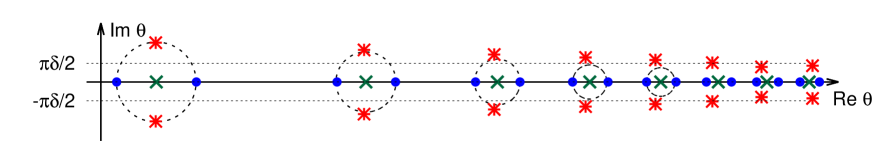
Figure 9: The arrangements of the Bethe roots solving (5.4) with $N=16$, $p_{1}=p_{2}=0$ and $|\delta|=0.05$. The (green) crosses show the roots $\{u_{\ell}\}$, (blue) dots show the roots $\{\theta_{\mathscr{J}}\}$ for $\delta>0$ and (red) asterisks show the (complex) roots $\{\theta_{\mathscr{J}}\}$ for $\delta<0$ (the roots $\{u_{\ell}\}$ remains the same). Only a part of complex plane, containing a half of the roots is shown. The dashed lines and circles illustrate the pairing of $\theta$-roots described by eqs. (5.8) and (5.11).

Using BAE (5.4) one can show [40] that the vacuum energy (5.6) diverges quadratically for large $N$ (cf. eq. (3.18))

$$\frac{RE}{\pi}=\epsilon_{2}\,N^{2}+{\epsilon}_{0}\,r^{2}\,\log\big{(}{4N/r}\big{)}+O(1)\ \ \ \qquad(N\to\infty)\,,$$ (5.12)

where

$$\epsilon_{2}=-(1+\delta)\,,\qquad{\epsilon}_{0}=-{\textstyle\frac{1}{\pi^{2}}}\ \cos^{2}\big{(}\textstyle{\frac{\pi\delta}{2}}\big{)}\,,\qquad r=MR\,.$$ (5.13)

Then from the finite-size scaling arguments (applied in the context of the Bethe ansatz regularization of massive field theory models [20, 21]) one expects that for $N\to\infty$  the regularized expression for the energy

$${\mathfrak{F}}(r,{\bf k})=-\frac{c_{\bf{k}}}{6}+\lim_{\scriptstyle{\begin{subarray}{c}N\to\infty\\ r-\mbox{\scriptsize{fixed}}\end{subarray}}}\left(\frac{RE}{\pi}-\epsilon_{2}\,N^{2}-{\epsilon}_{0}\,r^{2}\ \Big{(}\log({4N/r})+C\,\Big{)}\right)\,,$$ (5.14)

where $c_{\bf{k}}=\sum_{i=1}^{2}\big{(}1-6a_{i}k_{i}^{2}\big{)}$, reduces to the scaling function ${\mathfrak{F}}(r,{\bf k})$ for the integrable case of the QFT model (1.1), (1.2). The constant $C$ is non-universal, it is determined by the requirement ${\mathfrak{F}}(r,{\bf k})\to 0$ as $r\to\infty$. The relation (5.3) follows from the requirement that (5.14) has the same large distance decay exponent as in (3.29). For $\delta>0$ the formula (5.14) has been verified numerically. The values ${\mathfrak{F}}(r,{\bf k})$ obtained from (5.6) with the solution of (5.4a), (5.4b) and (5.9) for $N=500$ display a good agreement (to within at least three decimal places) with the more accurate results obtained from the NLIE (4.30), see Fig. 10.

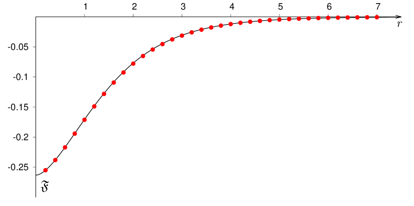
Figure 10: Dots show values of ${\mathfrak{F}}(r,{\bf k})$ for $\delta=17/47$, $p_{1}=1/10,p_{2}=1/20$ calculated from (5.6) and (5.14) with $N=500$ and the value of $C=0.9658605$. The continuous curve represents the results obtained from (4.33) and the NLIE (4.30).

Finally note that, as shown by Saleur [12], the BAE (5.4a), (5.4b), describing the $\delta>0$ vacuum state (5.9) filled by the real $\theta$-roots, can be converted to a set of NLIE. After some minor corrections these NLIE (generalized for the twisted boundary conditions (1.5)) can be written as

$$\tilde{\varepsilon}_{j}(\theta)={\tilde{r}}_{j}\,\sinh(\theta)-2\pi{\tilde{k}}_{j}+\sum_{l=1,2}\,\int_{-\infty}^{\infty}\frac{\mbox{d}\theta^{\prime}}{\pi}\ \widetilde{G}_{jl}(\theta-\theta^{\prime})\ \Im m\Big{[}\log\big{(}1+\mbox{e}^{-{\rm i}\tilde{\varepsilon}_{l}(\theta^{\prime}-{\rm i}0)}\big{)}\,\Big{]}\,,$$ (5.15)

where $j=1,2$,

$${\tilde{r}}_{1}=2r\,\cos\big{(}{\textstyle\frac{\pi\delta}{2}}\big{)}\,,\quad{\tilde{r}}_{2}=r\,,\quad{\tilde{k}}_{1}=k_{2}\,,\quad{\tilde{k}}_{2}=k_{+}\,,\quad k_{\pm}={\textstyle\frac{1}{2}}\,(k_{1}\pm k_{2})\,.$$ (5.16)

The kernel $\widetilde{G}_{jl}$ reads

$$\widetilde{G}_{11}(\theta)=\int_{-\infty}^{\infty}\,\mbox{d}\nu\ \frac{\mbox{e}^{{\rm i}\nu\theta}\,\sinh(\frac{\pi\nu a_{1}}{2})}{\sinh(\frac{\pi\nu a_{2}}{2})}\,,\qquad\widetilde{G}_{22}(\theta)=\int_{-\infty}^{\infty}\,\mbox{d}\nu\ \frac{\mbox{e}^{{\rm i}\nu\theta}\,\sinh^{2}(\frac{\pi\nu\delta}{2})}{\sinh(\frac{\pi\nu a_{1}}{2})\sinh(\frac{\pi\nu a_{2}}{2})}\,,$$ (5.17)

and

$$\widetilde{G}_{12}(\theta)=\widetilde{G}_{21}(\theta)=\int_{-\infty}^{\infty}\,\mbox{d}\nu\ \frac{\mbox{e}^{{\rm i}\nu\theta}\,\sinh(\frac{\pi\nu}{2})}{\sinh(\frac{\pi\nu a_{2}}{2})}\ .$$ (5.18)

Note that $\widetilde{G}_{22}(\theta)$ coincides with ${G}_{++}(\theta)$ defined in (4.31). With these notations the scaling function (5.14) can be written as

$${\mathfrak{F}}(r,{\bf k})=\frac{1}{\pi^{2}}\sum_{j=1,2}\,{\tilde{r}}_{j}\,\int_{-\infty}^{\infty}\,\mbox{d}\theta\,\sinh(\theta)\,\Im m\Big{[}\log\big{(}1+\mbox{e}^{-{\rm i}\tilde{\varepsilon}_{j}(\theta-{\rm i}0)}\big{)}\,\Big{]}\ .$$ (5.19)

$r=MR$	$\ \ \ \ \ \ \ {\mathfrak{F}}(r,{\bf k})$	$\ \ \ \ \ {\mathfrak{F}}(r,{\bf k})_{\rm UV}$	$\ \ \ \ \ {\mathfrak{F}}(r,{\bf k})_{\rm IR}$
$0.1$	$-0.2607428309788$	$-0.2607428313953$	$\ \ \ \ \ \ \ \ \star\star\star$
$0.2$	$-0.2549983506999$	$-0.2549983772536$	$\ \ \ \ \ \ \ \ \star\star\star$
$0.3$	$-0.2472190685352$	$-0.2472193690897$	$\ \ \ \ \ \ \ \ \star\star\star$
$0.4$	$-0.2380056043350$	$-0.2380072781157$	$\ \ \ \ \ \ \ \ \star\star\star$
$0.5$	$-0.2277756139968$	$-0.2277819263012$	$\ \ \ \ \ \ \ \ \star\star\star$
$0.6$	$-0.2168482299168$	$-0.2168668158811$	$\ \ \ \ \ \ \ \ \star\star\star$
$0.7$	$-0.2054791982549$	$-0.2055252929751$	$\ \ \ \ \ \ \ \ \star\star\star$
$0.8$	$-0.1938786835672$	$-0.1939794374587$	$\ \ \ \ \ \ \ \ \star\star\star$
$0.9$	$-0.1822213607225$	$-0.1824212140898$	$\ \ \ \ \ \ \ \ \star\star\star$
$1.0$	$-0.1706526112907$	$-0.1710196176110$	$-0.2014349564662$
$1.1$	$-0.1592926194023$	$-0.1599255303999$	$-0.1847842117398$
$1.2$	$-0.1482393124726$	$-0.1492751769847$	$-0.1692047325819$
$1.3$	$-0.1375706804828$	$-0.1391926693109$	$-0.1547042796504$
$1.4$	$-0.1273467826821$	$-0.1297919365909$	$-0.1412670230341$
$1.5$	$-0.1176116153451$	$-0.1211782235966$	$-0.1288603066874$
$1.6$	$-0.1083949276224$	$-0.1134492772872$	$-0.1174399287778$
$1.7$	$-0.0997140161108$	$-0.1066963026919$	$-0.1069542273502$
$1.8$	$-0.0915754934205$	$-0.1010047442851$	$-0.0973472061921$
$1.9$	$-0.0839770063651$	$-0.0964549329272$	$-0.0885608931075$
$2.0$	$-0.0769088715072$	$-0.0931226275591$	$-0.0805370881568$
$2.4$	$-0.0535707439372$	$\ \ \ \ \ \ \ \ \ \star\star\star$	$-0.0549560607657$
$2.8$	$-0.0369408994984$	$\ \ \ \ \ \ \ \ \ \star\star\star$	$-0.0374531791217$
$3.2$	$-0.0253532059419$	$\ \ \ \ \ \ \ \ \ \star\star\star$	$-0.0255388456222$
$3.6$	$-0.0173705422556$	$\ \ \ \ \ \ \ \ \ \star\star\star$	$-0.0174369596054$
$4.0$	$-0.0118987032850$	$\ \ \ \ \ \ \ \ \ \star\star\star$	$-0.0119222709924$
$4.4$	$-0.0081537173228$	$\ \ \ \ \ \ \ \ \ \star\star\star$	$-0.0081620342332$
$4.8$	$-0.0055903459505$	$\ \ \ \ \ \ \ \ \ \star\star\star$	$-0.0055932695721$
$5.2$	$-0.0038344869615$	$\ \ \ \ \ \ \ \ \ \star\star\star$	$-0.0038355117142$
$5.6$	$-0.0026307619638$	$\ \ \ \ \ \ \ \ \ \star\star\star$	$-0.0026311203213$
$6.0$	$-0.0018049899423$	$\ \ \ \ \ \ \ \ \ \star\star\star$	$-0.0018051150200$
$6.4$	$-0.0012382494264$	$\ \ \ \ \ \ \ \ \ \star\star\star$	$-0.0012382930098$
$6.8$	$-0.0008492127577$	$\ \ \ \ \ \ \ \ \ \star\star\star$	$-0.0008492279219$
$7.2$	$-0.0005821697868$	$\ \ \ \ \ \ \ \ \ \star\star\star$	$-0.0005821750559$
$7.6$	$-0.0003989064681$	$\ \ \ \ \ \ \ \ \ \star\star\star$	$-0.0003989082967$
$8.0$	$-0.0002731844458$	$\ \ \ \ \ \ \ \ \ \star\star\star$	$-0.0002731850797$
$8.4$	$-0.0001869773822$	$\ \ \ \ \ \ \ \ \ \star\star\star$	$-0.0001869776017$
$8.8$	$-0.0001278976621$	$\ \ \ \ \ \ \ \ \ \star\star\star$	$-0.0001278977381$
$9.2$	$-0.0000874328116$	$\ \ \ \ \ \ \ \ \ \star\star\star$	$-0.0000874328378$
$9.6$	$-0.0000597346969$	$\ \ \ \ \ \ \ \ \ \star\star\star$	$-0.0000597347060$
$10.$	$-0.0000407872423$	$\ \ \ \ \ \ \ \ \ \star\star\star$	$-0.0000407872454$

Table 1: Numerical data for Fig. 8. The first column contains numerical values of ${\mathfrak{F}}(r,{\bf k})$ obtained by solving the NLIE (4.30), (4.33) for $\delta=\frac{17}{47}=0.36\ldots,\ k_{1}=\frac{47}{150},\ k_{2}=\frac{47}{640}$. The second and third columns contain the short- and large-distance asymptotics of ${\mathfrak{F}}(r,{\bf k})$, given by (2.19) and (4.35), respectively.

Note, that even though the equations (5.15) look totally different from (4.30) the resulting expression (5.19) for the scaling function is, in fact, exactly equivalent to (4.33). A complete proof of this equivalence is presented in our next paper [40]. It is also worth noting that from the point of view of numerical analysis the system (4.30) displays a much faster convergence than (5.15) and, therefore, requires lesser computational resources. Moreover, the system (4.30) is well suited for small $\delta$ analysis, whereas the eq. (5.15) becomes singular for $\delta\to 0$ (the latter fact has already been noted in [12], where the NLIE (5.15) for the untwisted case $k_{\pm}=0$ were originally derived).

6 Conclusion

The Bukhvostov-Lipatov (BL) model [3] describes weakly interacting instantons and anti-instantons in the $O(3)$ non-linear sigma model in two dimensions. In this paper we have studied various aspects of the BL model with twisted boundary conditions, using all well-established approaches to 2D massive integrable QFT, including the conformal perturbation theory (Sec. 2), the standard renormalized perturbation theory (Sec. 3) and the Bethe ansatz (Sec. 5). Moreover, in Sec. 4 we have proposed an exact formula (4.29) for the vacuum energy of the model, expressing it via a special solution of the sinh-Gordon equation (4.24) in the domain ${\mathbb{D}}_{\rm BL}$ (see Fig. 7). The required solution $\hat{\eta}(w)$ decays at $|w|\to\infty$ and obey the boundary conditions (4.25) at the singular points $w_{1}$ and $w_{2}$. The connection to the classically integrable sinh-Gordon equation is rather powerful, since it allows one to obtain the non-linear integral equations (4.30), determining the vacuum energy in the form (4.33). We have shown that this formula perfectly matches all our perturbation theory calculations as well as the previously known coordinate Bethe ansatz results of Bukhvostov and Lipatov [3], and Saleur [12]. The comparisons were done both analytically (where possible) and numerically. Complete proofs and derivations of our exact results are postponed into the forthcoming publication [40]. The main idea of that work is to connect the functional equations for connection coefficients for the auxiliary linear problem for the sinh-Gordon equation (4.24) to the Bethe ansatz equations (5.2), arising from the coordinate Bethe ansatz [3]. This requires rather substantial works involving the particle-hole transformation and lattice-type regularization of the BAE, as well as some generalization of arguments of ref.[14], devoted to the Fateev model.

Clearly, further study of the BL model is desirable. Indeed, almost all the considerations in this paper concerns the weak coupling regime $0<\delta<1$. However, the most interesting regime is the strong coupling regime $\delta>1$, where the BL model admits a dual description as the so-called sausage model [10]. Interestingly, this model turns into the $O(3)$ NLSM, in the limit $\delta\to\infty$. This suggests that the instanton counting becomes exact in the strong coupling limit of the BL model. We intend to address this problem in the future.

The description of the vacuum state energy of the BL model in terms of the classical sinh-Gordon equation can be viewed as an instance of a remarkable, albeit unusual correspondence between integrable quantum field theories and integrable classical field theories in two dimensions, which cannot be expected from the standard quantum–classical correspondence principle. In the past two decades this topic has undergone various conceptual developments, which can be traced through the works [22, 23, 24, 27, 28, 25, 26, 29, 30, 13, 14, 31, 32]. The commonly accepted mystery of this correspondence is slightly unveiled by our conformal perturbation theory calculations in Sec. 2 and Sec. 4. Indeed eqs. (2.28) and (4.19), expressing the vacuum energy in terms of the solutions (4.13), (4.16) of the Liouville equation (4.17) arise as a direct result of calculations, without any additional assumptions. It would be interesting to check whether these calculations can be generalized to other integrable QFTs where the correspondence to classical integrable equations is known. More generally, it would be very important to better understand connections of the above correspondence to mathematical structures arising in 4D gauge theories [33, 34, 35], calculations of amplitudes of high energy scattering [36, 37, 38] and dualities in finite dimensional quantum-mechanical systems [39].

References

[1]
A. M. Polyakov and A. A. Belavin, “Metastable states of two-dimensional
isotropic ferromagnets”, JETP Lett.22 (1975) 245–248
[Pisma Zh. Eksp. Teor. Fiz. 22, 503 (1975)]
[2]
V. A. Fateev, I. V. Frolov and A. S. Schwarz, “Quantum fluctuations of
instantons in the nonlinear sigma model”,
Nucl. Phys.B154 (1979) 1–20
[3]
A. P. Bukhvostov and L. N. Lipatov, “Instanton—anti-instanton interaction in
the nonlinear -model and an exactly soluble fermion
theory”, Nucl.
Phys.B180 (1981) 116
[4]
M. Lüscher, “Does the topological susceptibility in lattice sigma models
scale according to the perturbative renormalization group?”,
Nucl. Phys.B200 (1982) 61–70
[5]
M. Ameduri, C. J. Efthimiou and B. Gerganov, “On the integrability of the
Bukhvostov-Lipatov model”,
Mod. Phys. Lett.A14 (1999) 2341–2352
[arXiv:hep-th/9810184]
[6]
V. A. Fateev, “The sigma model (dual) representation for a two-parameter
family of integrable quantum field theories”,
Nucl. Phys.B473 (1996) 509–538
[7]
A. B. Zamolodchikov and Al. B. Zamolodchikov, “Factorized
-matrices in two dimensions as the exact solutions of certain
relativistic quantum field theory models”, Ann. Physics120 no. 2, (1979) 253–291
[8]
A. M. Polyakov and P. B. Wiegmann, “Theory of nonabelian
Goldstone bosons in two dimensions”,
Phys. Lett.B131 (1983) 121–126
[9]
L. D. Faddeev and N. Yu. Reshetikhin, “Integrability of the
Principal Chiral Field model in (1+1)-dimension”,
Annals Phys.167 (1986) 227
[10]
V. A. Fateev, E. Onofri and A. B. Zamolodchikov, “The sausage model
(integrable deformations of sigma model)”,
Nucl. Phys.B406 (1993) 521–565
[11]
G. V. Dunne and M. Unsal, “Resurgence and trans-series in quantum field
theory: The model”,
JHEP11
(2012) 170
[arXiv:1210.2423]
[12]
H. Saleur, “The long delayed solution of the Bukhvostov-Lipatov model”,
J. Phys.A32 (1999) L207
[arXiv:hep-th/9811023]
[13]
S. L. Lukyanov, “ODE/IM correspondence for the Fateev model”,
JHEP12
(2013) 012
[arXiv:1303.2566]
[14]
V. V. Bazhanov and S. L. Lukyanov, “Integrable structure of Quantum Field
Theory: Classical flat connections versus quantum stationary states”,
JHEP09
(2014) 147
[arXiv:1310.4390]
[15]
V. V. Bazhanov, G. A. Kotousov and S. L. Lukyanov, “Winding vacuum energies in
a deformed sigma model”,
Nucl. Phys.B889 (2014) 817–826
[arXiv:1409.0449]
[16]
A. B. Zamolodchikov, “Painleve III and 2-d polymers”,
Nucl. Phys.B432 (1994) 427–456
[arXiv:hep-th/9409108]
[17]
F. Lesage, H. Saleur and P. Simonetti, “Tunneling in quantum wires: Exact
solution of the spin isotropic case”,
Phys. Rev.B56 (1997) 7598–7606 [arXiv:cond-mat/9703220]
[18]
V. A. Fateev, “The duality between two-dimensional integrable field theories
and sigma models”,
Phys. Lett.B357 (1995) 397–403
[19]
A. B. Zamolodchikov and A. B. Zamolodchikov, “Structure constants and
conformal bootstrap in Liouville field theory”,
Nucl. Phys.B477 (1996) 577–605
[arXiv:hep-th/9506136]
[20]
C. Destri and H. J. De Vega, “Unified approach to thermodynamic Bethe
Ansatz and finite size corrections for lattice models and field theories”,
Nucl. Phys.B438 (1995) 413–454
[arXiv:hep-th/9407117]
[21]
S. L. Lukyanov, “Critical values of the Yang-Yang functional in the
quantum sine-Gordon model”,
Nucl. Phys.B853 (2011) 475–507
[arXiv:1105.2836]
[22]
P. Dorey and R. Tateo, “Anharmonic oscillators, the thermodynamic Bethe
ansatz and nonlinear integral equations”, J. Phys. A32
no. 38, (1999) L419–L425 [arXiv:hep-th/9812211]
[23]
V. V. Bazhanov, S. L. Lukyanov and A. B. Zamolodchikov, “Spectral
determinants for Schrodinger equation and Q-operators of conformal field
theory”, J. Statist.
Phys.102 (2001) 567–576
[arXiv:hep-th/9812247]
[24]
J. Suzuki, “Functional relations in Stokes multipliers: Fun with potential”, J.
Statist. Phys.102 (2001) 1029–1047
[arXiv:quant-ph/0003066]
[25]
V. V. Bazhanov, S. L. Lukyanov and A. B. Zamolodchikov, “Higher level
eigenvalues of Q operators and Schroedinger equation”,
Adv. Theor. Math.
Phys.7 no. 4, (2003) 711–725
[arXiv:hep-th/0307108]
[26]
D. Fioravanti,
“Geometrical loci and CFTs via the Virasoro symmetry of the mKdV-SG hierarchy: An excursus,”
Phys. Lett. B609 (2005) 173-179
[arXiv:hep-th/0408079]
[27]
P. Dorey, C. Dunning, D. Masoero, J. Suzuki and R. Tateo,
“Pseudo-differential equations, and the Bethe ansatz for the classical Lie
algebras”, Nucl. Phys.B772 (2007) 249–289
[arXiv:hep-th/0612298]
[28]
B. Feigin and E. Frenkel, “Quantization of soliton systems and Langlands
duality”
[arXiv:0705.2486]
[29]
S. L. Lukyanov and A. B. Zamolodchikov, “Quantum sine(h)-Gordon model and
classical integrable equations”,
JHEP07
(2010) 008
[arXiv:1003.5333]
[30]
P. Dorey, S. Faldella, S. Negro and R. Tateo, “The Bethe Ansatz and the
Tzitzeica-Bullough-Dodd equation”,
Phil. Trans. Roy. Soc.
Lond.A371 (2013) 20120052
[arXiv:1209.5517]
[31]
D. Masoero, A. Raimondo and D. Valeri, “Bethe ansatz and the spectral theory
of affine Lie algebra-valued connections I. The simply-laced case”,
Commun. Math. Phys.344 no. 3, (2016) 719–750
[arXiv:1501.07421]
[32]
K. Ito and C. Locke, “ODE/IM correspondence and Bethe ansatz for affine Toda
field equations”,
Nucl. Phys.B896 (2015) 763–778
[arXiv:1502.00906]
[33]
D. Gaiotto, G. W. Moore and A. Neitzke, “Wall-crossing, Hitchin systems, and
the WKB Approximation”
[arXiv:0907.3987]
[34]
N. A. Nekrasov and S. L. Shatashvili, “Quantization of integrable systems and
four dimensional gauge theories”, in Proceedings, XVIth International
Congress on Mathematical Physics, Prague, 2009, pp. 265–289, World
Scientific: 2010
[arXiv:0908.4052]
[35]
A. V. Litvinov, “On spectrum of ILW hierarchy in conformal field theory”,
JHEP11
(2013) 155
[arXiv:1307.8094]
[36]
L. F. Alday, D. Gaiotto and J. Maldacena, “Thermodynamic Bubble Ansatz”,
JHEP09
(2011) 032
[arXiv:0911.4708]
[37]
B. Basso, A. Sever and P. Vieira, “Spacetime and flux tube -matrices at
finite coupling for supersymmetric Yang-Mills theory”,
Phys. Rev.
Lett.111 no. 9, (2013) 091602
[arXiv:1303.1396]
[38]
J. Bartels, L. N. Lipatov and A. Sabio Vera, “BFKL Pomeron, Reggeized gluons
and Bern-Dixon-Smirnov amplitudes”,
Phys. Rev.D80 (2009) 045002
[arXiv:0802.2065]
[39]
A. Mironov, A. Morozov, B. Runov, Y. Zenkevich and A. Zotov, “Spectral
duality between Heisenberg chain and Gaudin model”,
Lett. Math. Phys.103 no. 3, (2013) 299–329
[arXiv:1206.6349]
[40]
V. V. Bazhanov, S. L. Lukyanov and B. A. Runov, “Bukhvostov-Lipatov model
and quantum/classical duality”,
work in preparation (2016)