Superconductivity from Doublon Condensation in the Ionic Hubbard Model

Abstract

In the ionic Hubbard model, the onsite repulsion $U$, which drives a Mott insulator and the ionic potential $V$, which drives a band insulator, compete with each other to open up a window of charge fluctuations when $U\sim V$. We study this model on square and cubic lattices in the limit of large $U$ and $V$, with $V\sim U$. Using an effective Hamiltonian and a slave boson approach with both doublons and holes, we find that the system undergoes a phase transition as a function of $V$ from an antiferromagnetic Mott insulator to a paramagnetic insulator with strong singlet correlations, which is driven by a condensate of “neutral” doublon-hole pairs. On further increasing $V$, the system undergoes another phase transition to a superconducting phase driven by condensate of “charged” doublons and holes. The superfluid phase, characterized by presence of coherent (but gapped) fermionic quasiparticle, and $hc/e$ flux quantization, has a high $T_{c}\sim t$ which shows a dome shaped behaviour as a function of $V$. The paramagnetic insulator phase has a deconfined U(1) gauge field and associated gapless photon excitations. We also discuss how these phases can be detected in the ultracold atom context.

A dramatic observable effect of strong interactions between fermions on a lattice is the formation of Mott insulating states, where charge motion is suppressed due to large on-site repulsion Mott ; Imada_rev . This effect occurs in a large class of materials like transition metal oxides Mott_ins_expt1 ; Mott_ins_expt2 ; Mott_ins_expt3 ; Mott_ins_expt4 , including parent compounds of cuprate high $T_{c}$ superconductors Mott_ins_expt3 ; Mott_ins_expt4 . Recently, Mott insulators have been observed in systems of ultracold fermions on optical lattices MI_cold1 ; MI_cold2 , where the repulsive Fermi Hubbard model with tuneable Hamiltonian parameters can be implemented faithfully.

A theoretically challenging problem is to ascertain the fate of a system in proximity to a Mott insulator, where charge fluctuations are induced by different means; e.g. by doping the system away from commensurate filling (high $T_{c}$ cuprate superconductors) Lee_rev ; Plain_vanilla or by changing ambient pressure (organic superconductors) Org_Sc or simply by changing the ratio of the interaction energy scale to the kinetic energy scale (ultracold atomic systems) Cold_atom_cf . Experimentally, when charge fluctuation is induced around a Mott insulator, competing order parameters lead to a very rich phase diagram cuprate_comp_order ; Org_Sc with an ubiquitous presence of superconducting phases randARPES ; cuprate_Sc ; Org_Sc .

The Ionic Hubbard model is defined on bipartite lattices Hub_Torr , where, in addition to the kinetic energy ($\sim t$) and the local Hubbard repulsion ($\sim U$), the fermions are affected by a constant one-body potential difference between the two sublattices ($\sim V$). This model, originally proposed to explain ionic to neutral transitions  Hub_Torr ; Nagaosa , has also been used to describe ferroelectric transitions  ihm_ferro1 ; ihm_ferro2 ; ihm_ferro3 . It has recently been implemented in the context of ultracold atoms Esslinger_ihm where the relative strengths of $U$ and $V$ can be tuned controllably. In the absence of interactions, this model describes a band insulator at half-filling due to doubling of the unit cell, while, in the limit of strong interactions and weak potential, the system goes into the Mott insulating phase. While both $V$ and $U$, by themselves, promote insulating behaviour, they compete with each other leading to a window of charge fluctuations when they are comparable to each other.

In this Letter, we study the ionic Hubbard model in the limit of large $U$ and $V$, with $U\sim V$. The ionic Hubbard model has been studied in the literature using various techniques like exact diagonalization  ihm_ed , DMFT  ihm_DMFT1 ; ihm_DMFT2 ; ihm_DMFT3 ; ihm_DMFT4 ; ihm_DMFT5 and DMRG ihm_ed ; Manmana . Most of these works have focused on the regime $U\sim t$, where they have found an ionic to neutral transition in 1D and a metallic phase between a band insulator and a Mott insulator. In contrast, we will focus on $U\gg t$, so that we approach a charge fluctuation regime starting from a Mott insulator. For large $U/t$, Manmana et. al Manmana have studied the model in 1D using DMRG, while a slave boson approach has been used in the limit of small $V/U$ ihm_sbmft .

We use a new canonical transformation to derive an effective dimer-dipole Hamiltonian for $U/t$, $V/t$ $\gg 1$, with $U\sim V$, and study its phase diagram at $T=0$ at half-filling within a slave boson mean field theory. Our key results are: (i) Fermions hop by converting a spin-singlet on a bond to a charge dipole, with a doublon and a hole on the two sublattices, inducing charge fluctuation. (ii) Since the kinetic energy prefers spin-singlets, the antiferromagnetic order decreases with increasing $V$ and vanishes at a critical potential $V_{c1}$. (iii) Beyond a critical $V_{c2}$ the doublons and holes forming the dipole on the bond delocalize, leading to their Bose condensation. This creates a superconducting state with $hc/e$ vortices. (iv) The superfluid stiffness and critical temperature of this phase shows a non-monotonic dome shaped behaviour as a function of $V$. (v) At large $U$, $V_{c2}>V_{c1}$ and the intervening phase is a paramagnetic insulator described by strong singlet fluctuations and a paired superfluid paired_SF1 ; paired_SF2 ; paired_SF3 of doublon-hole pairs. This phase shows deconfinement of gauge degrees of freedom, which enforce projection constraints in the system, and associated emergent gapless “photons” deconfined . At lower values of $U$, the system shows a first order transition from an AF insulator to a superconductor.

Low Energy Effective Hamiltonian: The ionic Hubbard Hamiltonian is given by $H=H_{0}+H_{T}$,

$$H_{0} = U\sum_{i}n_{i\uparrow}n_{i\downarrow}+\frac{V}{2}\sum_{i}(-1)^{i}n_{i}$$

$$H_{T} = -t\sum_{\langle ij\rangle\sigma}c^{\dagger}_{i\sigma}c_{j\sigma}=\sum_{n}T^{n}_{-}+T^{n}_{+}$$ (1)

Here $H_{0}$, the local part of the Hamiltonian, includes the ionic potential $\pm V/2$ on $B(A)$ sublattice. $T^{n}_{+(-)}$ hops a Fermion from the $A(B)$ to the $B(A)$ sublattice and increases the double occupancy by $n$, with $n=0,\pm 1$, causing an energy change $\Delta E^{n}_{s}=nU+Vs$. In the regime, $U\gg t$, $V\gg t$, $U-V\sim zt$, where $z$ is the co-ordination number, $T^{1}_{-}$ and $T^{-1}_{+}$ are low energy hoppings, even at half-filling. They create/annihilate a doublon-hole pair, i.e. a charge dipole on a bond, so that the Hubbard repulsion is offset by the potential energy gained in the process. The canonical transformation Macdonald ; smref1 then eliminates all high energy hopping processes and we obtain the low-energy effective Hamiltonian,

$$\tilde{H}=H_{0}+T^{1}_{-}+T^{-1}_{+}+\frac{1}{U+V}[T_{+}^{1},T_{-}^{-1}]+\frac{1}{V}[T_{+}^{0},T_{-}^{0}]$$ (2)

We note that this effective Hamiltonian is obtained by an expansion around the $U=V$ limit, and is notably different from the effective Hamiltonian obtained by perturbing around the $U\gg t,V\sim 0$ limit otherham . Our effective Hamiltonian does not contain terms $\sim 1/(U-V)$, i.e. the resonant processes encountered in the expansion around $V=0$ are treated non-perturbatively (as ${\cal O}(t)$ hopping terms) in our approach. We will later see that this new hopping process kills antiferromagnetism and leads to a superconductivity of doublons and holes in this regime. The second order terms lead to spin-spin and density-density interactions, as well as intra-sublattice hopping terms. We will now use a slave boson mean-field theory to determine the phase diagram of this effective model.

Slave Boson Formalism: In the slave boson formalism slave_boson , the fermion operator $c^{\dagger}_{i\sigma}=f^{\dagger}_{i\sigma}h_{i}+\sigma f_{i\bar{\sigma}}d^{\dagger}_{i}$, where $f_{i\sigma}$ is a spin $1/2$ chargeless fermion (spinon), and holes $h_{i}$ and doublons $d_{i}$ are spinless bosons carrying opposite charge, $\pm 1$. The physical Hilbert space is obtained by imposing the constraint $d^{\dagger}_{i}d_{i}+h^{\dagger}_{i}h_{i}+\sum_{\sigma}f^{\dagger}_{i\sigma}f_{i\sigma}=1$ at every lattice site.

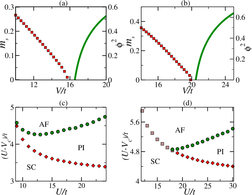
Figure 1: The staggered magnetization $m_{s}$ and the condensate fraction of the doublons (holes) $\phi^{2}$ as a function of the ionic potential $V$ for (a) square lattice with $U=20t$ and (b) cubic lattice with $U=25t$. (c) and (d): the phase diagram in the $U-V$ plane for (c) square lattice and (d) cubic lattice.

At low energies, the doublons are projected out of the $B$ sublattice and holes are projected out of $A$ sublattice as they cost an energy $\sim U$ footnote1 . The low energy degrees of freedom are $f_{iA(B)\sigma}$, $d_{iA}$ and $h_{iB}$, with the constraints $d^{\dagger}_{iA}d_{iA}+\sum_{\sigma}f^{\dagger}_{iA\sigma}f_{iA\sigma}=1$ and $h^{\dagger}_{iB}h_{iB}+\sum_{\sigma}f^{\dagger}_{iB\sigma}f_{iB\sigma}=1$ to be implemented by Lagrange multipliers $\mu^{A}$ and $\mu^{B}$ respectively. The effective Hamiltonian is

$$\tilde{H} = \sum_{i}\mu^{d}_{i}n^{d}_{iA}+\mu^{h}_{i}n^{h}_{iB}+\mu^{f}_{iA}n^{f}_{iA}+\mu^{f}_{iB}n^{f}_{iB}$$

$$-t \sum_{\langle ij\rangle\sigma}\sigma f_{jB\overline{\sigma}}f_{iA\sigma}d^{\dagger}_{iA}h^{\dagger}_{jB}+h.c$$

$$+ \frac{2t^{2}}{U+V}\sum_{\langle ij\rangle}\left[\vec{S}_{i}\cdot\vec{S}_{j}-\frac{1}{4}n^{f}_{i}n^{f}_{j}\right]+\frac{2t^{2}}{V}\sum_{\langle ij\rangle}n^{d}_{iA}n^{h}_{jB}$$

where $\mu^{d}_{i}=U-V-2\mu-\mu^{A}_{i}$, $\mu^{h}_{i}=-\mu^{B}_{i}$, $\mu^{f}_{iA}=-V/2-\mu-\mu^{A}_{i}$ and $\mu^{f}_{iB}=V/2-\mu-\mu^{B}_{i}$, and $\mu$ is the chemical potential. The low energy ${\cal O}(t)$ hopping term is a process which converts a spinon-singlet on a bond to a charge dipole (doublon-hole pair) on the bond and vice versa. The super-exchange interaction has a reduced scale of $2t^{2}/(U+V)\sim t^{2}/U$, while there is a nearest neighbour repulsion ${\cal O}(t^{2}/V)$ between a doublon and a hole smref1 .

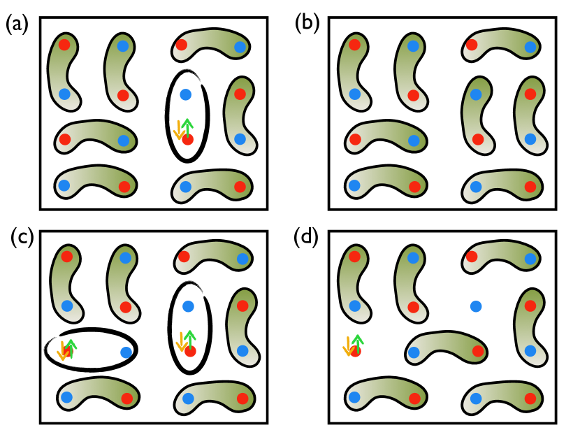
Figure 2: Schematic showing delocalization of doublons and holes. Red (blue) dots denote $A(B)$ sublattice, and the green bonds are spin-singlets: (a) A dipole is created in the background of singlets (b) At low density of dipoles, it fluctuates back to a singlet (c) At high density of dipoles a neighbouring bond can fluctuate to create a $d-h$ pair (d) The doublon of one dipole and the hole of another dipole creates a singlet, leaving a delocalized doublon and hole.

Mean Field Theory and the Phase Diagram: We first treat the effective Hamiltonian within a mean field theory, where the constraints are maintained on the average. We give mean field expectation value to staggered magnetization $m_{s}=\sigma\tau\langle f^{\dagger}_{i\tau\sigma}f_{i\tau\sigma}\rangle$, where $\tau=\pm 1$ for $A(B)$ sublattice, the doublon hole pairing amplitude $c_{1}=\langle d_{iA}h_{jB}\rangle$ and the spinon singlet amplitude $c_{2}=\sigma\langle f_{iA\sigma}f_{jB\overline{\sigma}}\rangle$, while the condensation of individual doublons/holes are indicated by the condensate fraction $\phi^{2}$.

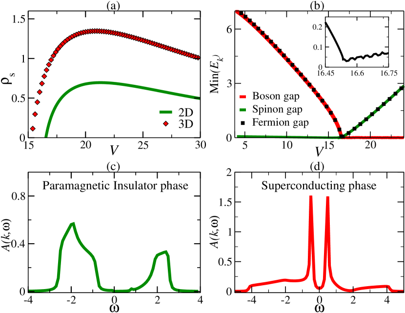
Figure 3: (a) The superfluid stiffness as a function of $V$ for the square and the cubic lattice. (b) The single particle fermion gap together with the spinon and the doublon/hole gap as a function of $V$. The inset shows that the gap always remains finite. (c) and (d): ${\cal A}(k,\omega)$ as a function of energy $\omega$ for $k=[\pi/2,\pi/2]$ in (c) the paramagnetic insulator and (d) the superconducting phase.

There are three distinct phases that are obtained within the slave-boson mean-field theory: (i) an antiferromagnetic (AF) Mott insulator at small $V$ (ii) a superconducting (SC) phase with a Bose condensate of linear combination of doublons and holes when $V\sim U$ and (iii) an intervening paramagnetic insulator (PI) which is a paired superfluid of doublon-hole pairs. A charge order exists in all the phases, but it does not correspond to any spontaneously broken symmetry for the ionic Hubbard model.

The AF order parameter $m_{s}$ is shown as a function of $V$ in Fig. 1 for large for (a) square ($U=20t$) and a (b) cubic lattice ($U=25t$). It decreases monotonically with $V$ and vanishes at $V=V_{c1}$ through a weakly first order transition. This can be understood from the fact that the kinetic energy favours spin-singlets which fluctuate to form charge dipoles on the bond and the energy cost of forming these dipoles is decreasing with increasing $V$. The subsequent dynamics of doublons and holes are explained schematically in Fig. 2. If the density of doublon-hole pairs are low, the dipoles fluctuate back to spin singlets before they can delocalize, leading to a paired superfluid with local charge fluctuations, as shown in Fig. 2 (a) and (b). If the density of dipoles is high, and there are dipoles on two neighbouring bonds, the doublon of one dipole and the hole of the other dipole can fluctuate back to a singlet leaving a separated doublon and hole, as shown in Fig. 2 (c) and (d). We note that this process can be easily visualized in the cold atom context through a quantum gas microscope Cold_atom_cf , which measures the local number parity in the system. In the PI phase, the even parity sites should occur in pairs, while the condensed phase would have a large number of isolated even parity sites. Fig. 1 (a) and (b) also shows the condensate fraction $\phi^{2}$ as a function of $V$, which is finite beyond a $V_{c2}>V_{c1}$, leading to a SC phase of delocalized condensed charged bosons. In the region $V_{c1}<V<V_{c2}$, the system is a paramagnetic insulator with short range spinon singlets ($c_{2}\neq 0$) and local doublon-hole pairs ($c_{1}\neq 0$, $\phi=0$) . Fig. 1 (c) and (d) shows the phase diagram in the $U-V$ plane for the square (c) and the cubic (d) lattice respectively. At low $U$, there is a first order transition between the AF state and the SC state, while at larger $U$, there is a weakly first order transition at $V_{c1}$ where the AF order vanishes and a continuous transition at $V_{c2}$ to the SC phase. The later transition should be in the $XY$ universality class paired_SF1 .

Gauge Transformations and the phases: The projection of the slave-boson states to the physical Hilbert space through local constrains leads to the following gauge invariance of the ionic Hubbard model: a $U(1)_{+}$ gauge transform, under which $f_{iA\sigma}\rightarrow f_{iA\sigma}e^{i\theta_{+}(i)},d_{iA}\rightarrow d_{iA}e^{i\theta_{+}(i)},f_{iB\sigma}\rightarrow f_{iB\sigma}e^{i\theta_{+}(i)},h_{iB}\rightarrow h_{iB}e^{i\theta_{+}(i)}$ and a $U(1)_{-}$ invariance, under which $f_{iA\sigma}\rightarrow f_{iA\sigma}e^{i\theta_{-}(i)},d_{iA}\rightarrow d_{iA}e^{i\theta_{-}(i)},f_{iB\sigma}\rightarrow f_{iB\sigma}e^{-i\theta_{-}(i)},h_{iB}\rightarrow h_{iB}e^{-i\theta_{-}(i)}$. We note that for charged fermions, under electromagnetic gauge transformations, the doublons and holes transform according to $U(1)_{-}$ gauge due to their opposite charges.

The doublon-hole pairing and the spinon singlet amplitude have charge $2$ with respect to the $U(1)_{+}$ transformations and their finite expectation leads to gapping out the $U(1)_{+}$ gauge fields throughout the phase diagram. The current corresponding to the $U(1)_{-}$ fluctuations is

$$\vec{j}^{p}_{-} = -it\sum_{\langle ij\rangle}\vec{r}_{ij}\left[c_{2}d^{\dagger}_{iA}h^{\dagger}_{jB}+c_{1}\sigma f^{\dagger}_{iA\sigma}f^{\dagger}_{jB\overline{\sigma}}-h.c\right]$$ (4)

where $\vec{r}_{ij}=\vec{r}_{i}-\vec{r}_{j}$. In the PI phase, the current response is given by $\chi^{j_{\alpha}j_{\beta}}+D^{\alpha\beta}$, with $D^{\alpha\beta}=-t\sum_{\langle ij\rangle}\vec{r}_{ij}^{\alpha}\vec{r}_{ij}^{\beta}[c_{2}d^{\dagger}_{iA}h^{\dagger}_{jB}+c_{1}\sigma f^{\dagger}_{iA\sigma}f^{\dagger}_{jB\overline{\sigma}}+h.c.]$. $D^{\alpha\alpha}$ goes to zero as $q\rightarrow 0,\omega\rightarrow 0$, leading to a paramagnetic insulator with neutral vortices consisting of doublons and holes flowing in the same direction. The PI phase has deconfined $U(1)_{-}$ gauge configurations with associated emergent gapless “photon” excitations. Beyond mean-field and RPA, the deconfined phase can: (i) confine due to instanton processes in 2D (ii) lead to a $Z_{2}$ gauge theory due to intra-sublattice hoppings or (iii) break further lattice symmetries. In principle, additional terms in the Hamiltonian can force a single smooth transition from the AF to the SC phase, where coupling to the critical matter fields can lead to a stable deconfined phase for the gauge fields. We note that our dimer-dipole model closely resembles a model studied earlier by Moessner et. al Moessner .

In the Bose condensed phase of the doublons/holes, the mode that condenses is a linear combination of $d^{\dagger}_{k}$ and $h_{-k}$ and has a $U(1)_{-}$ charge of $1$. The condensation of this charged mode leads to a superconducting response smref1 with a superfluid stiffness

$$\rho_{s}=(2z-4)tc_{2}\phi^{2}$$ (5)

The superfluid stiffness, plotted as a function of $V$ in Fig 3(a), scales with $t$ and shows a non-monotonic dependence on $V$. As $V$ increases, the condensate fraction $\phi^{2}$ increases, while the singlet amplitude $c_{2}$ decreases, since increase in doublon density is compensated by decrease in spinon density. The stiffness, which is a product of these two, thus shows non-monotonic behaviour. For the superconducting phase, $T_{c}\sim t$ and will follow the dome-shape of the stiffness as a function of $V$, reminiscent of the dependence of superconducting $T_{c}$ of cuprate superconductors with doping. Further, the destruction of the superconducting phase due to vortex proliferation at finite temperatures would lead to a phase with doublon-hole pairing showing pseudogap behaviour.

The SC phase is characterized by the presence of a linear superposition of Cooper pairing and $\eta$ pairing etapair , which creates doublons on $A$ and holes on $B$ sublattice. The vortices in this phase consist of doublons and holes moving in opposite directions around the vortex core, resulting in charge currents. In this picture, the charge $1$ of the vortices has a simple interpretation in terms of charge $2$ objects (pair of original fermions) flowing through one sublattice, rather than more exotic topological states Subir_vortex . In 3D, the presence of both the pair condensate and single particle condensate will lead to non-trivial drag effects and topological excitations sftopo_1 ; sftopo_2 ; sftopo_3 .

Single Particle Spectral Function: The spectral function ${\cal A}(k,\omega)$, which is the probability density of finding a fermion with a given momentum $k$ and energy $\omega$ contains detailed information about the single particle excitations in a system, and is a key measurable quantity both in material and cold- atom systems. Although the theory is formulated in terms of spinons and doublons/holes, the measurable quantity is the spectral function of the original $c$ fermions which is a convolution of the spectral function of the spinons and the bosons.

In the AF insulator phase the spinons are gapped on the scale of the superexchange interaction $\sim t^{2}/(U+V)$. The kinetic energy, on the other hand, leads to an extended s-wave pairing of the spinons ${\cal O}(t)$, where the gap function has a line node along the magnetic Brillouin zone. The spectral gap for spinons is shown in Fig. 3 (b). It goes down with $V$ as AF order weakens and would have gone to zero if there was a continuous transition. Instead, a first order transition intervenes, and on the other side, the spectral gap increases rapidly, driven by the chemical potential, as in the BEC limit of a BCS-BEC crossover BCSBEC . For the bosons, the quasiparticle spectrum has a minimum at the zone center. The spectral gap steadily decreases with $V$ till it reaches zero at $V_{c2}$ and remains zero in the condensed phase. The gap for the $c$ fermions is a sum of the two gaps and remains finite, as shown in the inset of Fig. 3(b). The gap is non-monotonic, dominated by the bosonic gap at small $V$ and by the spinon gap near $V\sim U$, with a minimum around $V_{c1}$.

In Fig. 3 (c) and (d), we plot ${\cal A}(k,\omega)$ for the square lattice system, at $k=[\pi/2,\pi/2]$, which corresponds to the minimum gap point in this case. In the AF and PI phase, the spectral function is completely incoherent, while the condensate leads to a coherent piece of the spectral function, with a residue proportional to the condensate fraction. The appearance of coherence peaks in the single particle spectral function can then be used to track the superconducting transition in this system experimentally.

Conclusion: We have studied the ionic Hubbard model on the square and cubic lattice, in the limit of large $U$ and large $V$, when $V\sim U$. Using a low energy dimer-dipole model and slave boson mean-field theory, we find that the AF order weakens with increasing $V$ and vanishes at a critical $V_{c1}$. At larger $V\sim U$, the system becomes a superconductor, driven by condensation of charged doublons and holes. This state is characterized by a coherent but gapped spectral function and a superfluid stiffness, which is non-monotonic as a function of $V$. This state, which has a dome shaped $T_{c}\sim t$, will also show pseudogap behaviour as temperature is raised above $T_{c}$. At large $U$, there is a paramagnetic insulating phase between the AF insulator and the superconductor, which, within the mean-field theory, is a gauge deconfined phase with its associated gapless excitations. This phase can be understood as a paired superfluid phase of doublons and holes. In ultracold atomic systems, the superfluid phase is easily detectable either through single particle spectral function measurements, or through quantum microscope, which can directly measure the delocalization of doublons and holes in real space.

Supplementary Material for: Superconductivity from Doublon Condensation in Ionic Hubbard Model

I Canonical Transformation and Low Energy Effective Hamiltonian

In a system, whose Hilbert space is fragmented into sectors of energy width $\sim\omega_{l}$ separated by a large energy scale $\omega_{h}$, a canonical transformation can be used to obtain the effective low energy Hamiltonian in each sector. The effective Hamiltonian is given by

$$\tilde{H} = e^{iS}He^{-iS}=H+[iS,H]+\frac{[iS,[iS,H]]}{2!}+....$$ (6)

where $iS$ has a strong coupling perturbation series in $\omega_{l}/\omega_{h}$ and is chosen in a way that the transformed Hamiltonian $\tilde{H}$ does not have any term connecting states belonging to different sectors order by order in $\omega_{l}/\omega_{h}$. The ionic Hubbard Hamiltonian is given by $H=H_{0}+H_{T}$,

$$H_{0} = U\sum_{i}n_{i\uparrow}n_{i\downarrow}+\frac{V}{2}\sum_{i}(-1)^{i}n_{i}$$

$$H_{T} = -t\sum_{\langle ij\rangle\sigma}c^{\dagger}_{i\sigma}c_{j\sigma}=\sum_{n}T^{n}_{-}+T^{n}_{+}$$ (7)

Here $H_{0}$ is the local part of the Hamiltonian, which includes both the Hubbard repulsion and the ionic potential. On the $A$ sublattice, single fermion states have energy $-V/2$, doublons have energy $U-V$ and holes have $0$ energy. On the $B$ sublattice, single fermion states have energy $V/2$, doublons have energy $U+V$ and holes have $0$ energy. $T^{n}_{+(-)}$ hops a Fermion from the $A(B)$ to the $B(A)$ sublattice and increases the double occupancy by $n$, with $n=0,\pm 1$. The action of $T^{n}_{s}$ on a configuration causes an energy change $\Delta E^{n}_{s}=nU+Vs$, which can be written as $[H_{0},T^{n}_{s}]=\Delta E^{n}_{s}T^{n}_{s}$.

In the resonant regime, $U-V$ is a low energy, while $U+V$ and $V$ are large energies. So the strong coupling expansion is obtained in powers of $t/(U+V)$ and $t/V$. In this case, it is clear that ${H_{T}}^{l}=\big{(}T_{-}^{1}+T_{+}^{-1}\big{)}$ are low energy hopping terms causing energy change $\sim U-V$, while the terms ${H_{T}}^{h}={H_{T}}-{H_{T}}^{l}$ should be eliminated by canonical transformation. This is achieved by

$$iS^{(1)}=\frac{1}{U+V}\left(T_{+}^{1}-T_{-}^{-1}\right)+\frac{1}{V}\left(T_{+}^{0}-T_{-}^{0}\right)$$ (8)

Out of the second order terms generated, it is clear that products of the form $T^{n}_{s}T^{-n}_{\overline{s}}$ brings the system back to the sector it started from, and would survive in second order, while the rest should be eliminated. This is achieved by

$$iS^{(2)} = \frac{1}{2(U+2V)}\left(\frac{1}{U+V}-\frac{1}{V}\right)\left([T^{1}_{+},T^{0}_{+}]+[T^{-1}_{-},T^{0}_{-}]\right)+\frac{1}{2U}\left(\frac{1}{U+V}+\frac{1}{V}\right)\left([T^{1}_{+},T^{0}_{-}]+[T^{-1}_{-},T^{0}_{+}]\right)$$

$$+\frac{1}{2U}\frac{1}{U+V}\left([T^{1}_{+},T^{1}_{-}]+[T^{-1}_{-},T^{-1}_{+}]\right)+\frac{1}{2V}\frac{1}{U+V}\left([T^{-1}_{-},T^{1}_{-}]+[T^{1}_{+},T^{-1}_{+}]\right)$$

$$-\frac{1}{UV}\left([T^{1}_{-},T^{0}_{+}]+[T^{-1}_{+},T^{0}_{-}]\right)+\frac{1}{V(U-2V)}\left([T^{1}_{-},T^{0}_{-}]+[T^{-1}_{+},T^{0}_{+}]\right)$$

The effective low energy Hamiltonian upto second order ($t^{2}/U$) in the perturbation expansion takes the following form :

$$\tilde{H} = H_{0}+H_{T}+[iS^{(1)},H_{0}+H_{T}]+[iS^{(2)},H_{0}]+\frac{1}{2}[iS^{(1)},[iS^{(1)},H_{0}]]$$ (10)

$$= H_{0}+\left(T_{-}^{1}+T_{+}^{-1}\right)+\frac{1}{U+V}\left[T_{+}^{1},T_{-}^{-1}\right]+\frac{1}{V}\left[T^{0}_{+},T^{0}_{-}\right]$$

II Effective Hamiltonian Using Slave Boson Operators

In the slave boson formalism, the fermion operator $c^{\dagger}_{i\sigma}$ is written in terms of spinful fermions (spinons) $f^{\dagger}_{i\sigma}$ and charged bosons, doublons $d^{\dagger}_{i}$ with charge $+1$ and holons $h^{\dagger}_{i}$ with charge $-1$. This is given by $c^{\dagger}_{i\sigma}=f^{\dagger}_{i\sigma}h_{i}+\sigma f_{i\overline{\sigma}}d^{\dagger}_{i}$ along with the constraint equation $f^{\dagger}_{i\sigma}f_{i\sigma}+d^{\dagger}_{i}d_{i}+h^{\dagger}_{i}h_{i}=1$. In the resonant regime, configurations with doublons on $B$ sublattice and holons on $A$ sublattice are projected out of the low energy subspace and hence we can write $c^{\dagger}_{iA\sigma}=\sigma f_{iA\overline{\sigma}}d^{\dagger}_{iA}$ and $c^{\dagger}_{iB\sigma}=f^{\dagger}_{iB\sigma}h_{iB}$. The constraint equations are then given by $f^{\dagger}_{iA\sigma}f_{iA\sigma}+d^{\dagger}_{iA}d_{iA}=1$ and $f^{\dagger}_{iB\sigma}f_{iB\sigma}+h^{\dagger}_{iB}h_{iB}=1$. Using this, we can write different low energy hopping terms in the Hamiltonian in the following way :

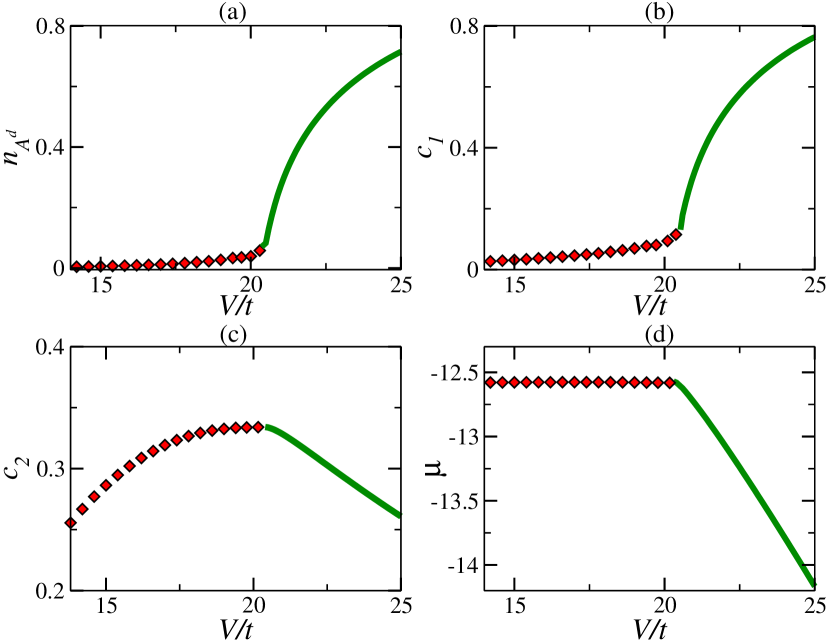
Figure 4: Different Mean field parameters as a function of the ionic potential $V$ for a cubic lattice with $U=25t$ (a) doublon number density ($n_{A}^{d}$) (b) doublon-hole pairing ($c_{1}$) (c) spin singlet pairing ($c_{2}$) (d) chemical potential ($\tilde{\mu}$).

$\mathcal{O}(t)$ hopping terms :

$$T^{1}_{-}+T^{-1}_{+} = -t\sum\limits_{\langle ij\rangle\sigma}\sigma f_{jB\bar{\sigma}}f_{iA\sigma}d_{iA}^{\dagger}h_{jB}^{\dagger}+h.c.$$ (11)

It is clearly seen that the low energy hopping process is equivalent to a spin singlet on a bond fluctuating to a doublon-holon pair (a charge dipole) and vice-versa.

$\mathcal{O}(t^{2}/U)$ terms involving sites on a single bond :

$$\frac{1}{U+V}\left[T^{1}_{+},T^{-1}_{-}\right] = \frac{2t^{2}}{U+V}\sum\limits_{\langle ij\rangle}\vec{S}_{i}\cdot\vec{S}_{j}-\frac{1}{4}n^{f}_{i}n^{f}_{j}$$ (12)

This is the usual superexchange term with a reduced superexchange scale $2t^{2}/(U+V)$. There is a factor of $2$ reduction since the intermediate virtual doublon can only be created on the $B$ sublattice (doublons on $A$ sublattice are low energy configurations). The other term is given by

$$\frac{1}{V}\left[T^{0}_{+},T^{0}_{-}\right] = -\frac{t^{2}}{V}\sum\limits_{\langle ij\rangle\sigma}\left[n_{iA}^{\sigma}n_{jB}^{h}+n_{iA}^{d}n_{jB}^{\bar{\sigma}}\right]$$ (13)

The attractive interaction between doublons/holes and spinons can alternatively be thought of as an effective repulsion between neighbouring doublons and holes by using the constraint equations to eliminate the spinons in these terms.
Intra-sublattice $\mathcal{O}(t^{2}/U)$ hopping terms : These terms are given by

$$\frac{t^{2}}{V}\sum\limits_{\langle ijl\rangle\sigma}\Big{[}\left(f^{\dagger}_{lA\sigma}f_{iA\sigma}n_{jB}^{\sigma}+f^{\dagger}_{lA\sigma}f_{iA\bar{\sigma}}f^{\dagger}_{jB\bar{\sigma}}f_{jB\sigma}\right)d^{\dagger}_{iA}d_{lA}$$

$$+\left(f^{\dagger}_{lB\sigma}f_{iB\sigma}n_{jA}^{\sigma}+f^{\dagger}_{lB\sigma}f_{iB\bar{\sigma}}f^{\dagger}_{jA\bar{\sigma}}f_{jA\sigma}\right)h^{\dagger}_{iB}h_{lB}\Big{]}$$ (14)

These terms describe the hopping doublon (holon) from a site to its next nearest neighbour site on same sublattice with an associated backflow of spinons. Note that the absence of doublons on $B$ sublattice and holes on $A$ sublattice precludes the possibility of a $t^{2}/(U+V)$ term of this kind. In addition to these terms, we use Lagrange multipliers $\mu_{i}^{A}$ and $\mu_{i}^{B}$ to implement the constraint on te two sublattices. In all the effective Hamiltonian can be written as

$$\tilde{H} = \sum_{i}\left[(U-V-2\mu-\mu_{i}^{A})n^{d}_{iA}-\mu_{i}^{B}n^{h}_{iB}\right]-\sum_{i}\left[\left(V/2+\mu+\mu_{i}^{A}\right)n^{f}_{iA}+\left(\mu+\mu_{i}^{B}-V/2\right)n^{f}_{iB}\right]$$ (15)

$$-t\sum_{\langle ij\rangle\sigma}\sigma\left(f_{jB\overline{\sigma}}f_{iA\sigma}d^{\dagger}_{iA}h^{\dagger}_{jB}+h.c.\right)+\frac{t^{2}}{U+V}\sum_{\langle ij\rangle\sigma}\left(-n_{iA}^{\sigma}n^{\bar{\sigma}}_{jB}+f_{iA\bar{\sigma}}^{\dagger}f_{iA\sigma}f_{jB\sigma}^{\dagger}f_{jB\bar{\sigma}}\right)-\frac{t^{2}}{V}\sum\limits_{\langle ij\rangle\sigma}\left(n_{iA}^{\sigma}n_{jB}^{h}+n_{iA}^{d}n_{jB}^{\sigma}\right)$$

$$+ \frac{t^{2}}{V}\sum\limits_{\langle ijl\rangle\sigma}\Big{[}\left(f^{\dagger}_{lA\sigma}f_{iA\sigma}n_{jB}^{\sigma}+f^{\dagger}_{lA\sigma}f_{iA\bar{\sigma}}f^{\dagger}_{jB\bar{\sigma}}f_{jB\sigma}\right)d^{\dagger}_{iA}d_{lA}+\left(f^{\dagger}_{lB\sigma}f_{iB\sigma}n_{jA}^{\sigma}+f^{\dagger}_{lB\sigma}f_{iB\bar{\sigma}}f^{\dagger}_{jA\bar{\sigma}}f_{jA\sigma}\right)h^{\dagger}_{iB}h_{lB}\Big{]}$$

III Mean Field Theory

We use a mean field theory where we decouple the bosons and fermions and the constraints are maintained on average. We take the following mean field parameters : the staggered magnetization $m_{s}=\frac{1}{2}\langle S_{iA}^{z}-S_{iB}^{z}\rangle$ where $S^{z}=\frac{1}{2}\langle f_{\uparrow}^{\dagger}f_{\uparrow}-f_{\downarrow}^{\dagger}f_{\downarrow}\rangle$, the singlet pairing amplitude $c_{2}=\langle\sigma f_{iA\sigma}f_{jB\bar{\sigma}}\rangle$, the doublon-holon pairing amplitude $c_{1}=\langle d_{iA}h_{jB}\rangle$. In addition we consider intra-sublattice hopping amplitude for both spinons and the bosons, $c_{3}=\langle f_{iA\sigma}^{\dagger}f_{lA\sigma}\rangle$ and $c_{4}=\langle d_{iA}^{\dagger}d_{lA}\rangle$. We note that individual spinon and boson densities are determined by the chemical potential and the Lagrange multipliers which implement the constraints. We have checked that out of different spatial symmetries for the pairing, the system always chooses extended s-wave pairing on energetic grounds.

At half-filling, charge neutrality forces equality between the doublon density $n^{d}$ and the holon density $n^{h}$. The constraint equations then imply that $n^{f}_{A}=n^{f}_{B}$, i.e. the spinon density on the two sublattices are equal. This gives us : $(U-V)-2\mu-\mu^{A}=-\mu^{B}$ and $-\mu-\mu^{A}-\frac{V}{2}=-\mu-\mu^{B}+\frac{V}{2}$, i.e. $\mu=\frac{U}{2}$, and $\mu^{B}-\frac{V}{2}=\mu^{A}+\frac{V}{2}=\tilde{\mu}$. This gives us a bosonic Hamiltonian

$$H^{B}=\sum\limits_{k}\left(\begin{array}[]{cc}d_{kA}^{\dagger}&h_{-kB}\end{array}\right)\left(\begin{array}[]{cc}a^{B}_{k}&-tc_{2}\gamma_{k}\\ -tc_{2}\gamma_{k}&a^{B}_{k}\end{array}\right)\left(\begin{array}[]{c}d_{kA}\\ h_{-kB}^{\dagger}\end{array}\right)$$ (16)

where, $a^{B}_{k}=-\tilde{\mu}-\frac{V}{2}-zJ_{3}n_{A}^{f}+\frac{1}{2}J_{3}(\gamma_{k}^{2}-z).(c_{3}n_{A}^{f}-c_{2}^{2})$, where $J_{1}=\frac{t^{2}}{U+V}$ and $J_{3}=\frac{t^{2}}{V}$ and $\gamma_{k}=2\sum\limits_{\alpha}\cos k_{\alpha}$. The Hamiltonian for fermions can be written as

$$H^{F}=\sum\limits_{k,\sigma}\left(\begin{array}[]{cc}f_{kA\sigma}^{\dagger}&f_{-kB\bar{\sigma}}\end{array}\right)\left(\begin{array}[]{cc}a^{F}_{k\sigma}&c^{F}_{k\sigma}\\ c^{F}_{F\sigma}&-a_{kF\sigma}\end{array}\right)\left(\begin{array}[]{c}f_{kA\sigma}\\ f_{-kB\bar{\sigma}}^{\dagger}\end{array}\right)$$ (17)

where, $a^{F}_{k\sigma}=-\tilde{\mu}-\frac{U}{2}-\frac{1}{2}zJ_{1}n_{A}^{f}-zJ_{1}\sigma m_{s}-zJ_{3}n^{d}+\frac{1}{2}J_{3}(\gamma_{k}^{2}-z)n_{B}^{f}c_{4}+\frac{1}{2}z(z-1)J_{3}c_{3}c_{4}$ and $c^{F}_{k\sigma}=-t\sigma\gamma_{k}c_{1}-\frac{1}{2}\sigma\gamma_{k}J_{1}c_{2}-J_{3}\sigma\gamma_{k}(z-1)c_{2}c_{4}$.

The bosonic Hamiltonian is diagonalized by a Bogoliubov transformation to yield the spectrum $E^{B}_{k}=\pm\sqrt{(a^{B}_{k})^{2}-t^{2}c_{2}^{2}\gamma_{k}^{2}}$, while the fermionic spectrum is given by $E^{F}_{k\sigma}=\pm\sqrt{(a^{F}_{k\sigma})^{2}+(c^{F}_{k\sigma})^{2}}$. If the bosonic spectrum reaches $0$ at any point on the Brillouin zone for a set of parameters, a condensate of the corresponding quasiparticles would form at that point. We have found that for s-wave symmetry of the doublon-hole pairing, this always occurs at the zone center. In that case, half-filling dictates that $\langle d^{\dagger}(0,0)\rangle=\langle h^{\dagger}(0,0)\rangle=\phi$ in 2D and $\langle d^{\dagger}(0,0,0)\rangle=\langle h^{\dagger}(0,0,0)\rangle=\phi$ in 3D, which the off-diagonal doublon-holon pairing terms fixing the relative phase of the condensate. In the condensed phase of the doublons and holons, the mean-field equations are

$$n_{A}^{d}=\phi^{2}+\frac{1}{N}\sum\limits_{k^{\prime}}\left[(u_{k}^{B})^{2}n_{B}(E_{k}^{B})+(v_{k}^{B})^{2}(1+n_{B}(E_{k}^{B}))\right]$$

$$m_{s}=\frac{1}{2N}\sum\limits_{k,\sigma}\sigma\left[(u_{k\sigma}^{F})^{2}n_{F}(E_{k\sigma}^{F})+(v_{k\sigma}^{F})^{2}\left(1-n_{F}(E_{k\sigma}^{F})\right)\right]$$

$$c_{1}=\phi^{2}-\frac{1}{zN}\sum\limits_{k^{\prime}}\gamma_{k}u_{k}^{B}v_{k}^{B}\left[1+2n_{B}(E_{k}^{B})\right]$$

$$c_{2}=\frac{1}{zN}\sum\limits_{k,\sigma}\bar{\sigma}\gamma_{k}u_{k\sigma}^{F}v_{k\sigma}^{F}\left[1-2n_{F}(E_{k\sigma}^{F})\right]$$

$$c_{3}=\frac{1}{z(z-1)N}\sum\limits_{k,\sigma}(\gamma_{k}^{2}-z)\left[(u_{k\sigma}^{F})^{2}n_{F}(E_{k\sigma}^{F})+(v_{k\sigma}^{F})^{2}\left(1-n_{F}(E_{k\sigma}^{F})\right)\right]$$

$$c_{4}=\phi^{2}+\frac{1}{z(z-1)N}\sum\limits_{k^{\prime}}(\gamma_{k}^{2}-z)\left[(u_{k}^{B})^{2}n_{B}(E_{k}^{B})+(v_{k}^{B})^{2}(1+n_{B}(E_{k}^{B}))\right]$$

$$n_{A}^{d}+\frac{1}{N}\sum\limits_{k,\sigma}\left[(u_{k\sigma}^{F})^{2}n_{F}(E_{k\sigma}^{F})+(v_{k\sigma}^{F})^{2}\left(1-n_{F}(E_{k\sigma}^{F})\right)\right]=1$$ (18)

where $k^{\prime}$ are the all other $k$ points except where condensation occurs and $n_{B}$ and $n_{F}$ are Bose function and Fermi function respectively. Bosonic coherence factors $u^{B}_{k}$ and $v^{B}_{k}$ are given by $(u_{k}^{B})^{2}=\frac{1}{2}\left(1+\frac{a_{k}^{B}}{E_{k}^{B}}\right)$ and $(v_{k}^{B})^{2}=\frac{1}{2}\left(\frac{a_{k}^{B}}{E_{k}^{B}}-1\right)$ respectively and the fermionic coherence factors $u^{F}_{k\sigma}$ and $v^{F}_{k\sigma}$ are given by $(u_{k\sigma}^{F})^{2}=\frac{1}{2}\left(1+\frac{a_{k\sigma}^{F}}{E_{k\sigma}^{F}}\right)$ and $(v_{k\sigma}^{F})^{2}=\frac{1}{2}\left(1-\frac{a_{k\sigma}^{F}}{E_{k\sigma}^{F}}\right)$ respectively. The equations for the uncondensed phase can be obtained by setting $\phi=0$. In the condensed phase, we use the additional equation $E^{B}_{k}(0,0)=0$ in 2D and $E^{B}_{k}(0,0,0)=0$ in 3D ensuring gaplessness of Goldstone modes.

The main features of the mean-field phase diagram together with the evolution of the order parameters $m_{s}$ and $\phi$ as a function of $V$ is discussed in the main text. The evolution of the other mean fields are shown in Fig. 4 for a cubic lattice with $U=25t$. The dotted points are in the phase where doublons are not condensed, whereas the condensed phase is shown with solid line. Fig.  4(a) and (b) show the doublon density and the doublon-holon pairing amplitude $c_{1}$. Both these quantities show a rapid rise in the condensed phase, with the transition point providing a point of inflection. Fig.  4(c) and (d) show the spinon pairing amplitude and the chemical potential. The spinon pairing increases as the system moves away from AF order and then decreases in the condensed phase as rapid increase of doublons force a smaller density of spinons in the system. The chemical potential also shows rapid changes with $V$ in the condensed phase, reflecting the changes in charged degrees of freedom.

IV Superfluid Stiffness

Within the slave boson mean field theory, the kinetic energy term coupled to a $U(1)_{-}$ gauge field is given by

$$H_{T} \rightarrow H_{T}(\vec{A})=-tc_{2}\sum\limits_{\langle ij\rangle}\left(d^{\dagger}_{iA}h^{\dagger}_{jB}e^{-i\vec{A}.(\vec{r_{i}}-\vec{r_{j}})}+h.c.\right)$$ (19)

$$-tc_{1}\sum\limits_{\langle ij\rangle\sigma}\sigma\left(f^{\dagger}_{iA\sigma}f^{\dagger}_{jB\bar{\sigma}}e^{-i\vec{A}.(\vec{r_{i}}-\vec{r_{j}})}+h.c.\right)$$

where, $\vec{A}$ is the corresponding vector potential. The paramagnetic current on a bond between $\vec{r}_{i}$ and $\vec{r}_{j}$ is

$$\vec{j^{p}_{-}}(q) = tc_{2}\sum\limits_{k}\left(\rho_{k+\frac{q}{2}}d^{\dagger}_{kA}h^{\dagger}_{-k-q,B}+h.c.\right)$$

$$+ tc_{1}\sum\limits_{k,\sigma}\sigma\left(\rho_{k+\frac{q}{2}}f^{\dagger}_{kA\sigma}f^{\dagger}_{-k-q,B\bar{\sigma}}+h.c.\right)$$ (20)

with $\rho_{k}=2\sum\limits_{\alpha}\sin{k_{\alpha}}$. The response of the system is given by

$$\langle(\vec{j_{-}^{p}}(q))_{\alpha}(\vec{j_{-}^{p}}(-q))_{\beta}\rangle+D^{\alpha\beta}(q)$$ (21)

where the diamagnetic response is given by

$$D^{\alpha\beta}(q\rightarrow 0) = t\sum_{k}\frac{\partial^{2}\gamma_{k}}{\partial k_{\alpha}\partial k_{\beta}}\Big{[}c_{2}\left(\langle d^{\dagger}_{kA}h^{\dagger}_{kB}\rangle+h.c.\right)$$ (22)

$$+c_{1}\sum\limits_{\sigma}\sigma\left(\langle f^{\dagger}_{kA\sigma}f^{\dagger}_{kB\bar{\sigma}}\rangle+h.c.\right)\Big{]}$$

In the non-condensed phase, the paramagnetic response is

$$\chi^{\alpha\alpha}(0) = t^{2}\sum\limits_{k}\left(\frac{\partial{\gamma_{k}}}{\partial k}\right)^{2}_{\alpha}\left[c_{2}^{2}\frac{(a^{B}_{k})^{2}}{(E^{B}_{k})^{3}}+c_{1}^{2}\frac{(a^{F}_{k\sigma})^{2}}{(E^{F}_{k})^{3}}\right]$$ (23)

while the diamagnetic response is given by

$$D^{\alpha\alpha} = -2t\sum\limits_{k}\frac{\partial^{2}{\gamma_{k}}}{\partial k_{\alpha}^{2}}\left[c_{2}u^{B}_{k}v^{B}_{k}+c_{1}\sum\limits_{\sigma}\sigma u^{F}_{k\sigma}v^{F}_{k\sigma}\right]$$ (24)

Using integration by parts, it can be easily shown that the paramagnetic and diamagnetic responses cancel each other exactly in the $q\rightarrow 0$ limit and hence the superfluid stiffness is $0$ in this phase. Note that the spinon and boson contributions cancel individually, and the system is an insulator.

In the condensed phase, the above calculation goes through, except for the fact that the condensation of the bosons add a new term to the current of the form

$$\delta\vec{j_{B-}^{p}}(q)=-tc_{2}\rho_{\frac{q}{2}}[\phi^{*}(d^{\dagger}_{-qA}+h_{qB})-\phi(h^{\dagger}_{-qB}+d_{qA})]$$ (25)

Working out the paramagnetic current-current correlator from this additional term we get

$$\delta\chi^{\alpha\alpha} = 4tc_{2}|\phi|^{2}$$ (26)

Similarly, the diamagnetic response gets an additional term

$$\delta D^{\alpha\alpha} = -2ztc_{2}|\phi|^{2}$$ (27)

Combining eqn.(26) and (27), we see that the contribution from paramagnetic and diamagnetic responses in the condensed phase do not cancel each other and we obtain the finite superfluid stiffness, $\rho_{s}=(2z-4)tc_{2}|\phi|^{2}$.

V Single Particle Spectral Functions

The single particle spectral function $\mathcal{A}(k,w)$, which is proportional to the imaginary part of the Green’s function, gives the probability density that a particle with a certain momentum $k$ has a specific energy $\omega$. The key point to note is that the original $c$ fermions constitute gauge invariant operators and hence their single particle Green’s functions will be measured by different experiments like ARPES, STS etc. Since the $c$ fermions are written as product of $f$ fermions and d/h bosons, the single particle Green’s function calculation for the $c$ fermions is akin to a bubble calculation of polarization function, with one fermion and one boson line forming the bubble. For example, the single particle fermion Green’s function for a up-spin fermion on $A$ sub-lattice is defined as :

$$\mathcal{G}_{AA}^{\uparrow}(i,j,\tau,\tau^{\prime})=-T_{\tau\tau^{\prime}}\left<c_{iA\uparrow}(\tau)c^{\dagger}_{jA\uparrow}(\tau^{\prime})\right>$$ (28)

$$= -T_{\tau\tau^{\prime}}\left[\left<f^{\dagger}_{iA\downarrow}(\tau)f_{jA\downarrow}(\tau^{\prime})\right>\left<d_{iA}(\tau)d^{\dagger}_{jA}(\tau^{\prime})\right>\right]$$

$$= D_{11}(\tau,\tau^{\prime})G^{\downarrow}_{11}(\tau^{\prime},\tau)$$

where, the angular bracket denotes the expectation value, $T$ is the time ordering operator, and the boson and spinon Green’s functions are given by

$$D(k,i\omega_{n})=\left(\begin{array}[]{cc}\frac{(u_{k}^{B})^{2}}{i\omega_{n}-E_{k}^{B}}-\frac{(v_{k}^{B})^{2}}{i\omega_{n}+E_{k}^{B}}&-u_{k}^{B}v_{k}^{B}\left(\frac{1}{i\omega_{n}-E_{k}^{B}}-\frac{1}{i\omega_{n}+E_{k}^{B}}\right)\\ \\ -u_{k}^{B}v_{k}^{B}\left(\frac{1}{i\omega_{n}-E_{k}^{B}}-\frac{1}{i\omega_{n}+E_{k}^{B}}\right)&\frac{(v_{k}^{B})^{2}}{i\omega_{n}-E_{k}^{B}}-\frac{(u_{k}^{B})^{2}}{i\omega_{n}+E_{k}^{B}}\end{array}\right)$$ (29)

$$G^{\sigma}(k,i\omega_{n})=\left(\begin{array}[]{cc}\frac{(u_{k\sigma}^{F})^{2}}{i\omega_{n}-E_{k\sigma}^{F}}+\frac{(v_{k\uparrow\sigma}^{F})^{2}}{i\omega_{n}+E_{k\sigma}^{F}}&-u_{k\sigma}^{F}v_{k\sigma}^{F}\left(\frac{1}{i\omega_{n}-E_{k\sigma}^{F}}-\frac{1}{i\omega_{n}+E_{k\sigma}^{F}}\right)\\ \\ -u_{k\sigma}^{F}v_{k\sigma}^{F}\left(\frac{1}{i\omega_{n}-E_{k\sigma}^{F}}-\frac{1}{i\omega_{n}+E_{k\sigma}^{F}}\right)&\frac{(v_{k\sigma}^{F})^{2}}{i\omega_{n}-E_{k\sigma}^{F}}+\frac{(u_{k\sigma}^{F})^{2}}{i\omega_{n}+E_{k\sigma}^{F}}\end{array}\right)\\$$

Fourier transforming to the momentum and Matsubara frequency space we get

$$\mathcal{G}_{AA}^{\uparrow}(k,i\omega_{n})=\sum\limits_{q}\frac{1}{\beta}\sum\limits_{iq_{l}}G_{11}^{\downarrow}(q,iq_{l})D_{11}(k+q,i\omega_{n}+iq_{l})$$ (30)

where $q_{l}=(2l+1)\pi T$, with integer $l$, is the fermionic Matsubara frequency. Working out the Matsubara sum, and taking the analytical continuation $i\omega_{n}\rightarrow\omega+i0^{+}$, we get the spectral function

$${\mathcal{A}_{AA}^{\uparrow}}(k,\omega)=\sum\limits_{q} \int\frac{d\omega^{\prime}}{\pi^{2}}\left[n_{F}(\omega^{\prime})+n_{B}(\omega^{\prime}+\omega)\right]$$ (31)

$$.(G^{\downarrow}_{11})^{\prime\prime}(q,\omega^{\prime})D_{11}^{\prime\prime}(q+k,\omega+\omega^{\prime})$$

where ^′′ denotes imaginary part of the Green’s function. Specializing to $T=0$, we get

$${\mathcal{A}_{AA}^{\uparrow}}(k,\omega)$$

$$=\sum\limits_{q}(u_{k+q}^{B})^{2}\Big{[}(v_{q\uparrow}^{F})^{2}\delta(\omega-E_{q\uparrow}^{F}-E_{k+q}^{B})\Theta(\omega-E_{q\uparrow}^{F})$$

$$+(u_{q\uparrow}^{F})^{2}\delta(\omega+E_{q\uparrow}^{F}+E_{k+q}^{B})\Theta(|\omega|-E_{q\uparrow}^{F})\Big{]}$$ (32)

In the bose condensed phase of the doublons, the spectral function picks up an additional contribution from the condensate given by

$${\mathcal{A}_{AA}^{\uparrow}}(k,\omega) = -\frac{1}{\pi}\phi^{2}(G^{\downarrow}_{11})^{\prime\prime}(k,\omega)$$

$$= \phi^{2}\left[(u_{k\uparrow}^{F})^{2}\delta(\omega-E_{k\uparrow}^{F})+(v_{k\uparrow}^{F})^{2}\delta(\omega+E_{k\uparrow}^{F})\right]$$

So, the zero temperature spectral function for fermion on $A$ sub-lattice are given as following :

$$\mathcal{A}_{AA}(k,\omega)=\sum\limits_{q,\sigma}\Big{[}(v_{q\sigma}^{F})^{2}(u_{k+q}^{B})^{2}\delta(\omega-E_{q\sigma}^{F}-E_{k+q}^{B})\Theta(\omega-E_{q\sigma}^{F})$$

$$+(u_{q\sigma}^{F})^{2}(v_{k+q}^{F})^{2}\delta(\omega+E_{q\sigma}^{F}+E_{k+q}^{B})\Theta(|\omega|-E_{q\sigma}^{F})\Big{]}+\phi^{2}\sum\limits_{\sigma}\left[(u_{k\sigma}^{F})^{2}\delta(\omega-E_{k\sigma}^{F})+(v_{k\sigma}^{F})^{2}\delta(\omega+E_{k\sigma}^{F})\right]$$

Similarly, we can calculate $\mathcal{A}_{BB}(k,\omega)$ and $\mathcal{A}_{AB}(k,\omega)$. The full single particle spectral function is given by $\mathcal{A}(k,\omega)=\mathcal{A}_{AA}(k,\omega)+\mathcal{A}_{BB}(k,\omega)+\mathcal{A}_{AB}(k,\omega)+\mathcal{A}_{BA}(k,\omega)$. It is clear that in the non-condensed phase the convolution gives rise to an incoherent spectral function. The gauge fluctuations, which will provide vertex corrections, will not change the incoherent nature of the spectral function. On the other hand, the condensate provides a coherent part to the spectral function, which is simply proportional to the spinon spectral function. Here, we see that the fermion spectral function has peaks at $|\omega|=E_{q\sigma}^{F}+E_{k+q}^{B}$, which corresponds to the gap of the spectral function and the minimum gap is given by $\omega_{c}=E_{k\sigma}^{F}(\pi/2,\pi/2)+E_{k}^{B}(0,0)$.

References

[1]
N. F. Mott.
Metal-insulator transition.
Rev. Mod. Phys., 40:677–683, Oct 1968.
[2]
Masatoshi Imada, Atsushi Fujimori, and Yoshinori Tokura.
Metal-insulator transitions.
Rev. Mod. Phys., 70:1039–1263, Oct 1998.
[3]
M. Z. Hasan, E. D. Isaacs, Z.-X. Shen, L. L. Miller, K. Tsutsui, T. Tohyama,
and S. Maekawa.
Electronic structure of mott insulators studied by inelastic x-ray
scattering.
Science, 288(5472):1811–1814, 2000.
[4]
Z.-X. Shen and D.S. Dessau.
Electronic structure and photoemission studies of late
transition-metal oxides — mott insulators and high-temperature
superconductors.
Physics Reports, 253(1):1 – 162, 1995.
[5]
Andrea Damascelli, Zahid Hussain, and Zhi-Xun Shen.
Angle-resolved photoemission studies of the cuprate superconductors.
Rev. Mod. Phys., 75:473–541, Apr 2003.
[6]
D. N. Basov and T. Timusk.
Electrodynamics of high- superconductors.
Rev. Mod. Phys., 77:721–779, Aug 2005.
[7]
Robert Jordens, Niels Strohmaier, Kenneth Gunter, Henning Moritz, and Tilman
Esslinger.
A mott insulator of fermionic atoms in an optical lattice.
Nature, 455:204–207, 09 2008.
[8]
U. Schneider, L. Hackermüller, S. Will, Th. Best, I. Bloch, T. A. Costi,
R. W. Helmes, D. Rasch, and A. Rosch.
Metallic and insulating phases of repulsively interacting fermions in
a 3d optical lattice.
Science, 322(5907):1520–1525, 2008.
[9]
Patrick A. Lee, Naoto Nagaosa, and Xiao-Gang Wen.
Doping a mott insulator: Physics of high-temperature
superconductivity.
Rev. Mod. Phys., 78:17–85, Jan 2006.
[10]
P W Anderson, P A Lee, M Randeria, T M Rice, N Trivedi, and F C Zhang.
The physics behind high-temperature superconducting cuprates: the
‘plain vanilla’ version of rvb.
Journal of Physics: Condensed Matter, 16(24):R755, 2004.
[11]
S. Lefebvre, P. Wzietek, S. Brown, C. Bourbonnais, D. Jérome, C. Mézière,
M. Fourmigué, and P. Batail.
Mott transition, antiferromagnetism, and unconventional
superconductivity in layered organic superconductors.
Phys. Rev. Lett., 85:5420–5423, Dec 2000.
[12]
Daniel Greif, Maxwell F. Parsons, Anton Mazurenko, Christie S. Chiu, Sebastian
Blatt, Florian Huber, Geoffrey Ji, and Markus Greiner.
Site-resolved imaging of a fermionic mott insulator.
Science, 351(6276):953–957, 2016.
[13]
Eduardo Fradkin, Steven A. Kivelson, and John M. Tranquada.
Colloquium : Theory of intertwined orders in high
temperature superconductors.
Rev. Mod. Phys., 87:457–482, May 2015.
[14]
J. C. Campuzano, M. Norman, and M. Randeria.
The physics of superconductors, vol. ii.
ed. by K. H. Bennemann and J. B. Ketterson, page 167, 2004.
[15]
J. G. Bednorz and K. A. Muller.
Possible high superconducitivity in the Ba-La-Cu-O
system.
Z. Phys. B, 64:189, April 1986.
[16]
J. Hubbard and J. B. Torrance.
Model of the neutral-ionic phase transformation.
Phys. Rev. Lett., 47:1750–1754, Dec 1981.
[17]
Naoto Nagaosa and Jun ichi Takimoto.
Theory of neutral-ionic transition in organic crystals. i. monte
carlo simulation of modified hubbard model.
Journal of the Physical Society of Japan, 55(8):2735–2744,
1986.
[18]
T. Egami, S. Ishihara, and M. Tachiki.
Lattice effect of strong electron correlation: Implication for
ferroelectricity and superconductivity.
Science, 261(5126):1307–1310, 1993.
[19]
R. Resta and S. Sorella.
Many-body effects on polarization and dynamical charges in a partly
covalent polar insulator.
Phys. Rev. Lett., 74:4738–4741, Jun 1995.
[20]
M. E. Torio, A. A. Aligia, and H. A. Ceccatto.
Phase diagram of the hubbard chain with two atoms per cell.
Phys. Rev. B, 64:121105, Sep 2001.
[21]
Michael Messer, Rémi Desbuquois, Thomas Uehlinger, Gregor Jotzu, Sebastian
Huber, Daniel Greif, and Tilman Esslinger.
Exploring competing density order in the ionic hubbard model with
ultracold fermions.
Phys. Rev. Lett., 115:115303, Sep 2015.
[22]
A P Kampf, M Sekania, G I Japaridze, and Ph Brune.
Nature of the insulating phases in the half-filled ionic hubbard
model.
Journal of Physics: Condensed Matter, 15(34):5895, 2003.
[23]
Arti Garg, H. R. Krishnamurthy, and Mohit Randeria.
Can correlations drive a band insulator metallic?
Phys. Rev. Lett., 97:046403, Jul 2006.
[24]
L. Craco, P. Lombardo, R. Hayn, G. I. Japaridze, and E. Müller-Hartmann.
Electronic phase transitions in the half-filled ionic hubbard model.
Phys. Rev. B, 78:075121, Aug 2008.
[25]
Krzysztof Byczuk, Michael Sekania, Walter Hofstetter, and Arno P. Kampf.
Insulating behavior with spin and charge order in the ionic hubbard
model.
Phys. Rev. B, 79:121103, Mar 2009.
[26]
Xin Wang, Rajdeep Sensarma, and Sankar Das Sarma.
Ferromagnetic response of a “high-temperature” quantum
antiferromagnet.
Phys. Rev. B, 89:121118, Mar 2014.
[27]
Arti Garg, H. R. Krishnamurthy, and Mohit Randeria.
Doping a correlated band insulator: A new route to half-metallic
behavior.
Phys. Rev. Lett., 112:106406, Mar 2014.
[28]
S. R. Manmana, V. Meden, R. M. Noack, and K. Schönhammer.
Quantum critical behavior of the one-dimensional ionic hubbard model.
Phys. Rev. B, 70:155115, Oct 2004.
[29]
B. J. Powell, J. Merino, and Ross H. McKenzie.
Ionic hubbard model on a triangular lattice for
, , and
: Mean-field slave boson theory.
Phys. Rev. B, 80:085113, Aug 2009.
[30]
Anatoly Kuklov, Nikolay Prokof’ev, and Boris Svistunov.
Superfluid-superfluid phase transitions in a two-component
bose-einstein condensate.
Phys. Rev. Lett., 92:030403, Jan 2004.
[31]
Anatoly Kuklov, Nikolay Prokof’ev, and Boris Svistunov.
Commensurate two-component bosons in an optical lattice: Ground state
phase diagram.
Phys. Rev. Lett., 92:050402, Feb 2004.
[32]
Ehud Altman, Walter Hofstetter, Eugene Demler, and Mikhail D Lukin.
Phase diagram of two-component bosons on an optical lattice.
New Journal of Physics, 5(1):113, 2003.
[33]
T. Senthil, Leon Balents, Subir Sachdev, Ashvin Vishwanath, and Matthew P. A.
Fisher.
Quantum criticality beyond the landau-ginzburg-wilson paradigm.
Phys. Rev. B, 70:144407, Oct 2004.
[34]
A. H. MacDonald, S. M. Girvin, and D. Yoshioka.
expansion for the hubbard model.
Phys. Rev. B, 37:9753–9756, Jun 1988.
[35]
See supplementary material for details.
[36]
The expansion around the limit yields a heisenberg model with a
modified superexchange scale ; see e.g.
[17].
[37]
T. Kopp, F. J. Seco, S. Schiller, and P. Wölfle.
Superconductivity in the single-band hubbard model: mean-field
treatment of slave-boson pairing.
Phys. Rev. B, 38:11835–11838, Dec 1988.
[38]
Placing holes on sublattice instead of sublattice gives an energy
gain of . this constraint will hold both at half-filling and low
hole doping, until the system cannot sustain all the holes on the
sublattice in the highly hole doped regime, which we do not consider here.
[39]
R. Moessner and S. L. Sondhi.
Irrational charge from topological order.
Phys. Rev. Lett., 105:166401, Oct 2010.
[40]
Chen Ning Yang.
pairing and off-diagonal long-range order
in a hubbard model.
Phys. Rev. Lett., 63:2144–2147, Nov 1989.
[41]
Subir Sachdev.
Stable hc / e vortices in a gauge theory of
superconductivity in strongly correlated systems.
Phys. Rev. B, 45:389–399, Jan 1992.
[42]
V. M. Kaurov, A. B. Kuklov, and A. E. Meyerovich.
Drag effect and topological complexes in strongly interacting
two-component lattice superfluids.
Phys. Rev. Lett., 95:090403, Aug 2005.
[43]
E. Smørgrav, E. Babaev, J. Smiseth, and A. Sudbø.
Observation of a metallic superfluid in a numerical experiment.
Phys. Rev. Lett., 95:135301, Sep 2005.
[44]
Egil V. Herland, Egor Babaev, and Asle Sudbø.
Phase transitions in a three dimensional
lattice london superconductor:
Metallic superfluid and charge- superconducting states.
Phys. Rev. B, 82:134511, Oct 2010.
[45]
Roberto B. Diener, Rajdeep Sensarma, and Mohit Randeria.
Quantum fluctuations in the superfluid state of the bcs-bec
crossover.
Phys. Rev. A, 77:023626, Feb 2008.