Large scale quantum walks by means of optical fiber cavities

Abstract

We demonstrate a platform for implementing quantum walks that overcomes many of the barriers associated with photonic implementations. We use coupled fiber-optic cavities to implement time-bin encoded walks in an integrated system. We show that this platform can achieve very low losses combined with high-fidelity operations, enabling an unprecedented large number of steps in a passive system, as required for scenarios with multiple walkers. Furthermore the platform is reconfigurable, enabling variation of the coin, and readily extends to multidimensional lattices. We demonstrate variation of the coin bias experimentally for three different values.

I Introduction

Quantum walks are the quantum counterparts to random walks. A quantum walker moves by superpositions of possible paths, resulting in a probability amplitude for being observed at a particular position Aharonov et al. (1993); Kempe (2003); Venegas-Andraca (2012). Quantum walks, both discrete-time and continuous-time, have been realized using cold atoms Preiss et al. (2015); Fukuhara et al. (2013), single optically trapped atoms Karski et al. (2009), trapped ions Schmitz et al. (2009); Xue et al. (2009); Zähringer et al. (2010), and photons. Optical multiport interferometers provide an attractive implementation for quantum walks, since optical fields naturally exhibit coherence between pathways and allow multi-walker scenarios using multiple single photons. Optical systems have been used to implement quantum walks using bulk optics Bouwmeester et al. (1999); Cardano et al. (2015), photonic chips Perets et al. (2008); Peruzzo et al. (2010); Sansoni et al. (2012); Crespi et al. (2013), fiber optics Regensburger et al. (2011), and hybrid bulk-fiber optic approaches Schreiber et al. (2010, 2011); Jeong et al. (2013). However, this approach is susceptible to losses, which both limit the achievable scale before being overtaken by detectors and background noise, and abrogate many of the advantages implied for applications in quantum information processing Childs et al. (2003); Childs and Goldstone (2004); Buhrman and Špalek (2006); Ambainis (2007, 2003); Shenvi et al. (2003); Kempe (2005); Magniez and Nayak (2007); Farhi et al. (2007). This challenge motivates the development of low-loss, modular, guided-wave interferometer networks for quantum walks.

Quantum walks with multiple interacting walkers have been shown to realize universal quantum computation Childs et al. (2013). Even with multiple non-interacting walkers, quantum walks are also thought to have quantum computational power, as illustrated by the boson sampling problem Aaronson and Arkhipov (2011). Quantum walks with a single walker can also implement quantum computation, though this requires an exponentially large graph Lovett et al. (2010); Childs (2009). A key feature of quantum walks as information processors is that they do not require time-dependent feedforward control.

In most experimental implementations, the quantum walk takes place over spatial locations arranged in a lattice. The physical size of the lattice then determines the maximum size of the walk. This limitation can be avoided by use of optical cavities, in which case the number of physical elements required is independent of the size of the walk. This approach was first formulated for frequency-encoded quantum walks Knight et al. (2003). From an experimental perspective, a further key advance was the development of optical cavities that implement time-encoded walks Schreiber et al. (2010); Regensburger et al. (2011). In this case, the walker’s location is represented by the time at which a pulse completes a round trip of a cavity Schreiber et al. (2010); Regensburger et al. (2011). In practice, the achievable scale of time-encoded walks is limited by optical loss incurred over each step. For hybrid schemes, an important challenge in this respect is the transition from bulk optics to fiber delays Nitsche et al. (2016). An alternate approach is complete fiber-integration, which has been developed and demonstrated with the use of optical amplifiers that counteract loss Regensburger et al. (2011). Amplification, however, prohibits potential extensions to single-photon and multi-walker applications.

In this paper, we implement time-encoded photonic quantum walks by means of passive fiber-integrated coupled optical cavities. We show that this platform achieves very low losses, reconfigurability, and high-fidelity operation over a large number of steps. In particular, we demonstrate one-dimensional coined walks of up to 62 steps with output fidelities over 0.99, for experiments with three values of coin bias in the same apparatus.

II Methods

Scheme– Our platform consists of pulsed light propagating in a network of optical ring cavities. The sizes and connectivity of the cavities can be chosen to design quantum walks with varying lattice geometry and walk rules. The simplest example, shown in Figure 1, is a coined one-dimensional quantum walk. This is achieved with two coupled cavities, which we label C₁ and C₂. These cavities have different round-trip times $T_{1}$ and $T_{2}$, which result in a round-trip delay difference $\tau=T_{2}-T_{1}>0$. The walker is represented by an optical pulse with duration much shorter than $T_{1}$, $T_{2}$, and $\tau$.

The walk begins when a pulse of light first reaches the inter-cavity coupler that connects C₁ and C₂. The role of this coupler is to coherently divide an incident pulse into two: one remaining in the same cavity and one transferred to the other. In terms of a coined quantum walk, the coupler carries out a coin flip, for which the state of the coin (heads or tails) is encoded in the position of the pulse (C₁ or C₂). Each subsequent round trip through the cavities constitutes a new step in the walk.

Propagation of the initial pulse in the coupled cavities generates a coherent train of pulses, with pulse-to-pulse separation $\tau$. The timing of each pulse encodes the location of the walker on a one-dimensional lattice. Interference occurs when indistinguishable paths create amplitudes for the same outcome. The first interference, for example, occurs when pulses generated from the initial state traverse C₁ and C₂ each once, albeit in a different order. These two trajectories correspond to paths in which the walker moves left then right, and vice versa.

The probability distribution corresponding to measurement of the walker’s position after $N$ steps is given by the relative energy of each pulse after $N$ round trips. Practically, this can be measured by coupling the cavities to an output waveguide by either an active switch or passive coupler. In the latter case, the distribution after every step can be sampled, at the cost of an effective loss that removes a fraction of the optical energy from the cavity in each step.

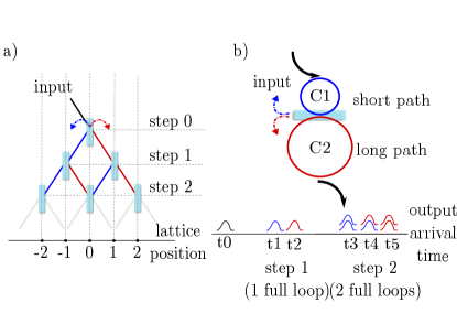
Figure 1: Optical implementations of a coined quantum walk over a one-dimensional lattice. (a) Beams propagating through a regular grid of beam splitters achieve a walk with spatial encoding. The powers of beams emerging from a grid of depth $N$ correspond to the probability distribution of the walker and coin (encoded in beam location and direction, respectively) after a walk of $N$ steps. (b) A pulse of light propagating through two coupled asymmetric ring cavities achieves a walk with time-bin and spatial encoding. The energy of pulses circulating in the cavities after $N$ round trips correspond to the walk distribution after $N$ steps. The two cavities correspond to orthogonal coin states, and timing of each pulse corresponds to the walker’s position.

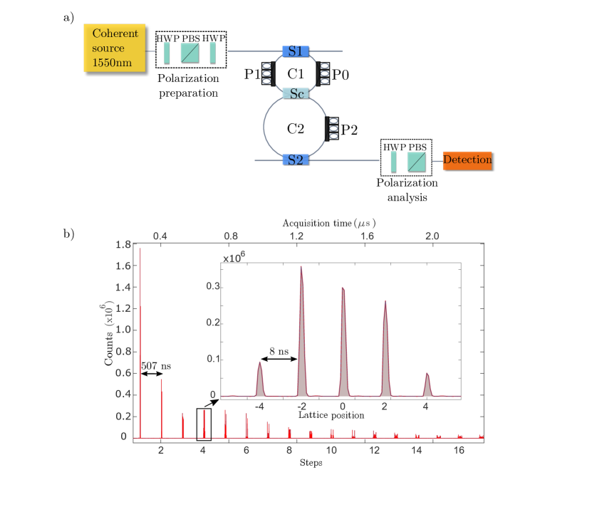
Figure 2: Schematic of the apparatus and representative data. (a) A 2.5-ns optical pulse is generated by a current-switched diode laser, passes through a polarization preparation stage consisting of half-wave plates (HWP) and a polarizing beam splitter (PBS), and couples into a two-cavity network via fiber coupler S₁. The two fiber-optic cavities C₁ and C₂ are joined by variable coupler S${}_{\textrm{c}}$ and connected by coupler S₂ to an output fiber leading to a polarization analysis stage and single-photon avalanche diode. The polarization controllers P₀, P₁, and P₂ compensate for polarization rotations in the non-polarization maintaining fiber-optic components. (b) Histogram of the detection time from $54\times 10^{6}$ trials, shown with 324 ps bins. The inset details the fourth step. Each peak is identified with a step number and lattice position according to its detection time, as described in the main text.

Experiment– Our apparatus is depicted in Figure 2a. First, a current-switched diode laser generates an optical pulse with a duration of 2.5 ns and a central wavelength of 1550 nm. A fraction of this pulse enters cavity C₁ through fused fiber coupler S₁, which has a reflectivity of 0.99. The cavities C₁ and C₂ are spliced together from standard telecommunications optical fiber (Corning SMF-28e) resulting in loop lengths (round-trip times) of 100.7 m (503 ns) and 102.2 m (511 ns), respectively. The round-trip time difference $\tau$ = 8 ns is chosen to be larger than the pulse duration, so that the resulting time bins are distinct. The cavities are connected through an evanescent-wave fiber coupler S${}_{\textrm{c}}$ (Evanescent Optics, model 905 SM non-PM) with a variable reflectivity $\eta_{\textrm{c}}$ corresponding to the coin bias.

Pulses circulating in C₂ are detected through the output fused fiber coupler S₂ with reflectivity 0.99. We choose the initial pulse energy so that the sum of all output pulses incident on the detector in one trial (i.e., all output pulses generated by one incident laser pulse) contains less than one photon on average. The pulse energies are then estimated using a single-photon avalanche diode with a time-to-digital converter that records the detection time relative to the initial pulse generation. Note that the timing window (162 ps) and detector jitter (300 ps) are much less than the pulse duration. Multiple trials are then used to estimate the mean photon number of each output pulse. We repeat trials every 33 $\upmu\textrm{s}$, which limits the detection range to 62 steps in each trial. The step limit would otherwise be determined by the cavity lengths, for which the pulse trains from consecutive steps overlap after step 65.

Non-polarization-maintaining optical fiber and fiber-optic components are used throughout the apparatus to minimize optical loss. To achieve high-quality interference, however, the polarization of the pulses must be controlled. In particular, the polarization rotations experienced in each cavity must commute so that, for example, the polarization of a pulse that traverses each cavity once is independent of the order in which it does so. Polarization control is achieved with three fiber paddle polarization controllers, labelled P₀, P₁ and P₂ in Figure 2a. These rotations are aligned using polarization preparation and analysis stages before and after the cavities and the first three transmitted pulses. After alignment, the polarization rotation errors over each cavity is measured to be less than 0.002 rad.

Representative data from 54$\times$10⁶ trials are shown in Figure 2a as a detection-time histogram. Time bins are observed as distinct peaks, each of which corresponds to a lattice position after a number of steps. Steps are identified as clusters of peaks that occur every 507 ns; lattice positions are identified as peaks within those clusters with peak-to-peak separation of 8 ns. To estimate the relative average energy of each pulse, we sum the counts in each peak, compensate for the detector reset time (which prohibits more than one detection event per trial), and subtract the average background measured between peaks. The optical loss per round trip in each cavity can then be readily determined from the exponential decay of pulses that circulate only in that cavity– i.e., pulses that correspond to an extremal lattice position for a given step number. We measure a round-trip excess loss, accounting for the reflectivities of the couplers, of 0.50 dB (0.47 dB) for C₁ (C₂). Finally, the normalized quantum walk outcome is calculated by dividing the energy of each pulse for a given step by the total energy of pulses in that step.

III Results

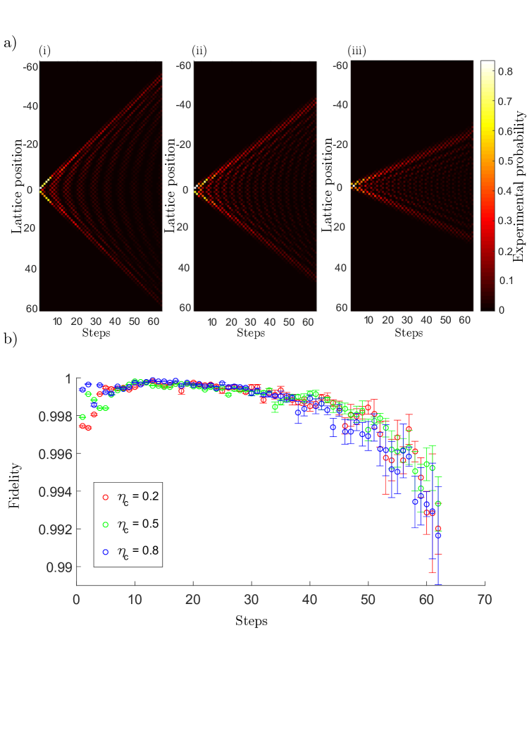
Figure 3: Experimental results for one-dimensional coined quantum walks. (a) Measured walk outcomes for 3 different values of coin bias: (i) $\eta_{\textrm{c}}=0.2$, (ii) $\eta_{\textrm{c}}=0.5$, and (iii) $\eta_{\textrm{c}}=0.8$ . (b) Fidelity of the experimental probability distribution with respect to that of an ideal quantum walk.

Figure 3a shows measured quantum walk outcomes for experiments with three values of coin bias $\eta_{\textrm{c}}$: 0.2, 0.5, and 0.8. We obtain precise estimates of the resulting probability distribution through step 62, the maximum that can be observed in our setup with the chosen trial repetition rate. Data for step 62 include approximately 9$\times$10³ detection events over 54$\times$10⁶ trials. For this final step, the largest uncertainty in probability of an outcome is 0.004 due to optical shot noise, and the smallest probability that could be resolved above background noise is 0.001.

These measured distributions show good agreement with those of an ideal quantum walk. In Figure 3b, we show the fidelity $F=\sum_{i}{\sqrt{P_{\textrm{exp}}(i)P_{\textrm{th}}(i)}}$ of the measured $\{P_{\textrm{exp}}(i)\}$ and theoretical $\{P_{\textrm{th}}(i)\}$ distribution at each step of the walk, where the lattice positions are specified by the index $i$. The fidelity of two distributions is 1 if they are identical and 0 if they are non-overlapping. We calculate $F>0.99$ for all observed steps in all experiments.

IV Discussion and Conclusions

We have presented a low-loss, flexible, passive fiber-optical platform for time-encoded quantum walks, and demonstrated its performance showing the longest one-dimensional walk yet observed. This platform benefits both from a cavity-based design, which allows the physical elements to be reused at each step, as well as practical advantages of entire fiber integration using high-quality components developed for telecommunications. We show that fiber polarization controllers can be used to precisely compensate for non-polarization-maintaining components, which allows for use of standard elements with minimal optical loss.

A number of technical improvements are possible for the system we demonstrate. The detector timing resolution and pulse duration can be brought below 100 ps, which would allow a decrease in time-bin separation by a factor of 30 from that used. This gain could be used, for example, to reduce the trial duration or increase the number of observable steps. We estimate that the optical loss per round trip can be readily reduced below the measured 0.5 dB by replacing couplers S₁ and S₂, which have excess loss of 0.3 dB with, for example, the variable evanescent-wave coupler used for S${}_{\textrm{c}}$, which has an excess loss below 0.1 dB, as well as an ability to set an optimal coupling ratio.

The use of fiber-integration with a spatially encoded coin allows our approach to be readily generalised to more complex networks of coupled cavities. Such configurations can be used to explore, for example, multi-dimensional lattices and different walk rules. For instance, a walk on a $D$-dimensional lattice can be achieved using $2D$ cavities with distinct round-trip times connected by a multiport coupler (see Figure 4). Additionally, polarization control can be included in walk design to access an additional degree of freedom. We also note that the relatively slow dynamics possible with long fiber lengths makes it possible to create a walk structure that depends on the step number and lattice position, as has been demonstrated in hybrid bulk-fiber setups Elster et al. (2015); Nitsche et al. (2016). A promising route for control within our all-fiber apparatus is strain-optic modulation Humphreys et al. (2014). The flexibility of the integrated fiber platform is in contrast to photonic chip approaches, which are limited in geometry and have not yet achieved reconfigurability in large waveguide arrays Schreiber et al. (2011); Crespi et al. (2013).

A future direction for this work, which we are now investigating, is studying the quantum interference of multiple single photons by connecting the input to a heralded single-photon source. This approach can enable the exploration of quantum walks with multiple walkers, and more generally, the study of time-encoded boson sampling He et al. (2016) and related Gaussian sampling problems Rahimi-Keshari et al. (2015).

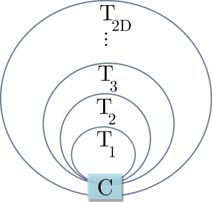
Figure 4: Schematic implementation of a quantum walk on a $D$-dimensional lattice using $2D$ ring cavities with distinct round-trip times. The coin flip is defined by the multiport coupler C connecting the cavities. Our experiment corresponds to $D=1$.

V Acknowledgements

We thank Eilon Poem, Joshua Nunn and Henry Wen for helpful discussions. J.B. and S.B. acknowledges support from the Marie Curie Actions within the Seventh Framework Programme for Research of the European Commission, under the Initial Training Network PICQUE (Photonic Integrated Compound Quantum Encoding, grant agreement no. 608062). S.B. acknowledges support from the European Union’s Horizon 2020 Research and Innovation program under Marie Sklodowska-Curie Grant Agreement No. 658073. I.A.W. acknowledges an ERC Advanced Grant (MOQUACINO) and the H2020-FETPROACT-2014 Grant QUCHIP (Quantum Simulation on a Photonic Chip; grant agreement no. 641039). M.S.K. acknowledge the European Research Council. I.A.W, M.S.K, and C.D.F. acknowledge the UK EPSRC project EP/K034480/1.

References

- Aharonov et al. (1993) Y. Aharonov, L. Davidovich, and N. Zagury, Phys. Rev. A 48, 1687 (1993).
- Kempe (2003) J. Kempe, Contemp. Phys. 44, 307 (2003).
- Venegas-Andraca (2012) S. E. Venegas-Andraca, Quantum Inf. Process. 11, 1015 (2012).
- Preiss et al. (2015) P. M. Preiss, R. Ma, M. E. Tai, A. Lukin, M. Rispoli, P. Zupancic, Y. Lahini, R. Islam, and M. Greiner, Science 347, 1229 (2015).
- Fukuhara et al. (2013) T. Fukuhara, P. Schauß, M. Endres, S. Hild, M. Cheneau, I. Bloch, and C. Gross, Nature 502, 76 (2013).
- Karski et al. (2009) M. Karski, L. Förster, J.-M. Choi, A. Steffen, W. Alt, D. Meschede, and A. Widera, Science 325, 174 (2009).
- Schmitz et al. (2009) H. Schmitz, R. Matjeschk, C. Schneider, J. Glueckert, M. Enderlein, T. Huber, and T. Schaetz, Phys. Rev. Lett. 103, 090504 (2009).
- Xue et al. (2009) P. Xue, B. C. Sanders, and D. Leibfried, Phys. Rev. Lett. 103, 183602 (2009).
- Zähringer et al. (2010) F. Zähringer, G. Kirchmair, R. Gerritsma, E. Solano, R. Blatt, and C. Roos, Phys. Rev. Lett. 104, 100503 (2010).
- Bouwmeester et al. (1999) D. Bouwmeester, I. Marzoli, G. P. Karman, W. Schleich, and J. P. Woerdman, Phys. Rev. A 61, 013410 (1999).
- Cardano et al. (2015) F. Cardano, F. Massa, H. Qassim, E. Karimi, S. Slussarenko, D. Paparo, C. de Lisio, F. Sciarrino, E. Santamato, R. W. Boyd, et al., Sci. Adv. 1, e1500087 (2015).
- Perets et al. (2008) H. B. Perets, Y. Lahini, F. Pozzi, M. Sorel, R. Morandotti, and Y. Silberberg, Phys. Rev. Lett. 100, 170506 (2008).
- Peruzzo et al. (2010) A. Peruzzo, M. Lobino, J. C. Matthews, N. Matsuda, A. Politi, K. Poulios, X.-Q. Zhou, Y. Lahini, N. Ismail, K. Wörhoff, et al., Science 329, 1500 (2010).
- Sansoni et al. (2012) L. Sansoni, F. Sciarrino, G. Vallone, P. Mataloni, A. Crespi, R. Ramponi, and R. Osellame, Phys. Rev. Lett. 108, 010502 (2012).
- Crespi et al. (2013) A. Crespi, R. Osellame, R. Ramponi, V. Giovannetti, R. Fazio, L. Sansoni, F. De Nicola, F. Sciarrino, and P. Mataloni, Nat. Photon. 7, 322 (2013).
- Regensburger et al. (2011) A. Regensburger, C. Bersch, B. Hinrichs, G. Onishchukov, A. Schreiber, C. Silberhorn, and U. Peschel, Phys. Rev. Lett. 107, 233902 (2011).
- Schreiber et al. (2010) A. Schreiber, K. N. Cassemiro, V. Potoček, A. Gábris, P. J. Mosley, E. Andersson, I. Jex, and C. Silberhorn, Phys. Rev. Lett. 104, 050502 (2010).
- Schreiber et al. (2011) A. Schreiber, K. Cassemiro, V. Potoček, A. Gábris, I. Jex, and C. Silberhorn, Phys. Rev. Lett. 106, 180403 (2011).
- Jeong et al. (2013) Y.-C. Jeong, C. Di Franco, H.-T. Lim, M. S. Kim, and Y.-H. Kim, Nat. Commun. 4, 2471 (2013).
- Childs et al. (2003) A. M. Childs, R. Cleve, E. Deotto, E. Farhi, S. Gutmann, and D. A. Spielman, in Proceedings of the 35th Annual ACM Symposium on Theory of Computing (ACM, 2003) pp. 59–68.
- Childs and Goldstone (2004) A. M. Childs and J. Goldstone, Phys. Rev. A 70, 022314 (2004).
- Buhrman and Špalek (2006) H. Buhrman and R. Špalek, in Proceedings of the seventeenth annual ACM-SIAM symposium on Discrete algorithm (Society for Industrial and Applied Mathematics, 2006) pp. 880–889.
- Ambainis (2007) A. Ambainis, SIAM J. Comput. 37, 210 (2007).
- Ambainis (2003) A. Ambainis, Int. J. Quantum Inf. 1, 507 (2003).
- Shenvi et al. (2003) N. Shenvi, J. Kempe, and K. B. Whaley, Phys. Rev. A 67, 052307 (2003).
- Kempe (2005) J. Kempe, Probab. Theory Related Fields 133(2), 215 (2005).
- Magniez and Nayak (2007) F. Magniez and A. Nayak, Algorithmica 48, 221 (2007).
- Farhi et al. (2007) E. Farhi, J. Goldstone, and S. Gutmann, arXiv:quant-ph/0702144 (2007).
- Childs et al. (2013) A. M. Childs, D. Gosset, and Z. Webb, Science 339, 791 (2013).
- Aaronson and Arkhipov (2011) S. Aaronson and A. Arkhipov, in Proceedings of the 43rd annual ACM symposium on Theory of computing (2011) pp. 333–342.
- Lovett et al. (2010) N. B. Lovett, S. Cooper, M. Everitt, M. Trevers, and V. Kendon, Phys. Rev. A 81, 042330 (2010).
- Childs (2009) A. M. Childs, Phys. Rev. Lett. 102, 180501 (2009).
- Knight et al. (2003) P. L. Knight, E. Roldán, and J. Sipe, Opt. Commun. 227, 147 (2003).
- Nitsche et al. (2016) T. Nitsche, F. Elster, J. Novotný, A. Gábris, I. Jex, S. Barkhofen, and C. Silberhorn, arXiv:1601.08204 (2016).
- Elster et al. (2015) F. Elster, S. Barkhofen, T. Nitsche, J. Novotný, A. Gábris, I. Jex, and C. Silberhorn, Sci. Rep. 5, 13495 (2015).
- Humphreys et al. (2014) P. C. Humphreys, B. J. Metcalf, J. B. Spring, M. Moore, P. S. Salter, M. J. Booth, W. S. Kolthammer, and I. A. Walmsley, Opt. Express 22, 21719 (2014).
- He et al. (2016) Y. He, Z. E. Su, H. Huang, X. Ding, J. Qin, C. Wang, S. Unsleber, C. Chen, H. Wang, Y. He, et al., arXiv:1603.04127 (2016).
- Rahimi-Keshari et al. (2015) S. Rahimi-Keshari, T. C. Ralph, and C. M. Caves, arXiv:1511.06526 (2015).