Thermal entanglement and sharp specific-heat peak in an exactly solved spin-1/2 Ising-Heisenberg ladder with alternating Ising and Heisenberg inter-leg couplings

Abstract

The spin-1/2 Ising-Heisenberg two-leg ladder accounting for alternating Ising and Heisenberg inter-leg couplings in addition to the Ising intra-leg coupling is rigorously mapped onto to a mixed spin-(3/2,1/2) Ising-Heisenberg diamond chain with the nodal Ising spins $S=3/2$ and the interstitial spin-1/2 Heisenberg dimers. The latter effective model with higher-order interactions between the nodal and interstitial spins is subsequently exactly solved within the transfer-matrix method. The model under investigation exhibits five different ground states: ferromagnetic, antiferromagnetic, superantiferromagnetic and two types of frustrated ground states with a non-zero residual entropy. A detailed study of thermodynamic properties reveals an anomalous specific-heat peak at low enough temperatures, which is strongly reminiscent because of its extraordinary height and sharpness to an anomaly accompanying a phase transition. It is convincingly evidenced, however, that the anomalous peak in the specific heat is finite and it comes from vigorous thermal excitations from a two-fold degenerate ground state towards a macroscopically degenerate excited state. Thermal entanglement between the nearest-neighbor Heisenberg spins is also comprehensively explored by taking advantage of the concurrence. The threshold temperature delimiting a boundary between the entangled and disentangled parameter space may show presence of a peculiar temperature reentrance.

I Introduction

In condensed matter physics, one of the most investigated subjects is the correlation between parts of composite systems fulde ; fazekas . In this sense, it is quite relevant to study the quantum part of these correlations, the so-called entanglement. Quantum entanglement is a fascinating feature of the quantum theory due to its nonlocal property bell . Therefore, many researchers have focused in recent years their attention to quantum entanglement as a potential resource for quantum computing and quantum information processing nielsen ; amicorev .

From the practical of view, there exist several real magnetic materials with obvious quantum manifestations as provided for instance by experimental representatives of the spin-1/2 quantum Heisenberg ladder batchelor . The most widespread families of the spin-1/2 Heisenberg ladder materials are cuprates Cu₂(C₅H₁₂N)₂Cl₄ chiari , SrCu₂O₃ Hiroi , (C₅H₁₂N)₂CuBr₄ willett , and vanadates M²⁺V₂O₅ Onoda , (VO)₂P₂O₇ barnes , which involve Cu²⁺ and V⁴⁺ magnetic ions as the spin-1/2 carriers. Recently, another experimental realization of the spin-1/2 Heisenberg two-leg ladder Cu(Qnx)(Cl_1-xBr_x)₂, where Qnx stands for quinoxaline (C₈H₆N₂), has opened up a new opportunity to continuously tune the inter-leg to intra-leg coupling ratio albeit in a relatively narrow range simutis .

Motivated by these experiments, a lot of interest has been devoted to theoretical investigation of the spin-1/2 Heisenberg ladder models batchelor . A large number of studies aimed at several variants of the Heisenberg spin ladder have addressed the ground-state properties amiri ; jaan-ladder . Besides, the existence of a magnetization plateau in the spin-1/2 Heisenberg ladder with alternating inter-leg exchange interactions was investigated by Paparidze and Pogosyan japaridze . There exist even a few generalized version of the $N$-leg spin-$S$ Heisenberg ladders Ramos , which were investigated using the density-matrix renormalization group method.

Frustrated spin ladders accounting for the crossing (next-nearest-neighbor) interaction were also intensively studied, some recent rigorous results for a ground-state phase diagram of the spin-1/2 Ising-Heisenberg ladder of this type can be found in Refs. strecka-ladders ; jozef-ladder-14 . Exact ground states were also found for a frustrated spin-1/2 Ising-Heisenberg ladder with the Heisenberg inter-leg coupling, the Ising intra-leg and crossing couplings. This model is in a certain limit equivalent to the spin-1/2 Ising-Heisenberg tetrahedral chain, which was also widely explored strecka-Vk-Ly ; strecka-lyra .

The spin-1/2 Ising-Heisenberg models being composed of the Ising (classical) and Heisenberg (quantum) spins vanden10 ; sahoo12 ; bellucci drew a special attention also from the experimental side as exemplified by numerous studies of the Ising-Heisenberg spin chains vanden10 ; sahoo12 ; bellucci ; hagiwara-strecka ; valverde08 ; ohanyan09 ; antonosyan09 ; canova09 ; rojas-ohanyan ; ana-roj ; strecka-jasc05 . In addition, the Ising-Heisenberg chains may display many intriguing and unexpected quantum properties valverde08 ; ohanyan09 ; antonosyan09 ; canova09 ; rojas-ohanyan ; spra such as thermal entanglement, intermediate plateaux in low-temperature magnetization curves antonosyan09 ; canova09 ; rojas-ohanyan or non-rational magnetization at zero temperature bellucci ; Ohanyan-prb15 .

In the present work, we will examine the spin-1/2 Ising-Heisenberg ladder with alternating Ising and Heisenberg inter-leg couplings. The organization of this paper is as follows. In Sec. 2 we will briefly describe the model under investigation and its rigorous mapping equivalence with the mixed-(3/2,1/2) Ising-Heisenberg diamond chain. We will also establish in Sec. 2 the relevant ground-state phase diagram. Sec. 3 deals with thermodynamics of the investigated model, whereas the particular attention is paid to a detailed study of temperature dependences of the specific heat and entropy. Sec. 4 is dedicated to the thermal entanglement between the nearest-neighbor Heisenberg spins. Finally, our conclusions are drawn in Sec. 5.

II Ising-Heisenberg ladder with alternating inter-leg interactions

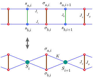
Figure 1: (Top) A schematic representation of the spin-1/2 Ising-Heisenberg ladder with alternating Ising and Heisenberg inter-leg interactions. Thick vertical lines correspond to the Heisenberg coupling ($J_{x},J_{z}$), while thin vertical and horizontal lines correspond to the Ising interactions $J_{0}$ and $J_{1}$; (Bottom) The equivalent mixed spin-(3/2,1/2) Ising-Heisenberg diamond chain with the nodal spin-3/2 Ising spins and the interstitial spin-1/2 Heisenberg dimers.

Let us consider the spin-1/2 Ising-Heisenberg ladder accounting for alternating Ising and Heisenberg inter-leg couplings in addition to the Ising intra-leg coupling, which is schematically depicted in figure 1. The Hamiltonian of the aforedescribed spin-1/2 Ising-Heisenberg ladder is given by

$$\mathcal{H}=\sum_{i=1}^{N}\left(H_{i}^{XXZ}+H_{i,i+1}^{I}+H_{i,i+1}^{IH}\right),$$ (1)

where

$$H_{i}^{XXZ}= -J_{x}(\sigma_{a,i}^{x}\sigma_{b,i}^{x}+\sigma_{a,i}^{y}\sigma_{b,i}^{y})-J_{z}\sigma_{a,i}^{z}\sigma_{b,i}^{z},$$ (2)

$$H_{i,i+1}^{I}= -\frac{J_{0}}{2}(s_{a,i}s_{b,i}+s_{a,i+1}s_{b,i+1}),$$ (3)

$$H_{i,i+1}^{IH}= -J_{1}(s_{a,i}+s_{a,i+1})\sigma_{a,i}^{z}-J_{1}(s_{b,i}+s_{b,i+1})\sigma_{b,i}^{z}.$$ (4)

In above, $\sigma_{\gamma,i}^{\alpha}$ denotes spatial components of the spin-1/2 operator ($\alpha=\{x,y,z\}$) at site $i$, and $\gamma=a$ or $b$ (see figure 1). The Ising inter-leg coupling is denoted by $J_{0}$, the Ising intra-leg coupling is denoted by $J_{1}$, while the anisotropic XXZ Heisenberg inter-leg coupling has two spatial components $J_{x}$ and $J_{z}$ in the $xy$-plane and along $z$-axis, respectively.

To proceed further with the calculation, let us proof a rigorous mapping equivalence between the spin-1/2 Ising-Heisenberg ladder defined through the total Hamiltonian (1) and the mixed spin-(3/2,1/2) Ising-Heisenberg diamond chain with the nodal spin-3/2 Ising spins and the interstitial spin-1/2 Heisenberg dimers as schematically illustrated in figure 1(bottom). The exact mapping relationship between both models can be proven by the use of the following spin identities nikolay

$$s_{a}(S)= \frac{13}{12}S-\frac{S}{3}^{3},$$ (5)

$$s_{b}(S)= \frac{7}{6}S-\frac{2S}{3}^{3},$$ (6)

which establish the exact mapping correspondence between the old spin-1/2 Ising variables $s_{a},s_{b}$ and the novel spin-3/2 Ising variable $S$

$$s_{a}= \frac{1}{2}, s_{b} =-\frac{1}{2} \qquad\Longleftrightarrow\qquad S=\frac{3}{2},$$ (7)

$$s_{a}= \frac{1}{2}, s_{b} =\frac{1}{2} \qquad\Longleftrightarrow\qquad S=\frac{1}{2},$$ (8)

$$s_{a}= -\frac{1}{2},\,\,\, s_{b} =-\frac{1}{2} \qquad\Longleftrightarrow\qquad S=-\frac{1}{2},$$ (9)

$$s_{a}= -\frac{1}{2}, s_{b} =\frac{1}{2} \qquad\Longleftrightarrow\qquad S=-\frac{3}{2}.$$ (10)

Consequently, the Hamiltonian parts (3) and (4) depending on the old spin-1/2 variables $s_{a},s_{b}$ can be rewritten in terms of the novel spin-3/2 Ising variables

$$H_{i,i+1}^{I}= J_{0}(\frac{S_{i}^{2}+S_{i+1}^{2}}{8}-\frac{5}{16}),$$ (11)

$$H_{i,i+1}^{IH}= J_{1}\left(\sigma_{a,i}^{z}+2\sigma_{b,i}^{z}\right)\frac{S_{i}^{3}+S_{i+1}^{3}}{3}$$

$$-J_{1}\left(13\sigma_{a,i}^{z}+14\sigma_{b,i}^{z}\right)\frac{S_{i}+S_{i+1}}{12}.$$ (12)

In this way, one establishes a rigorous mapping equivalence between the spin-1/2 Ising-Heisenberg ladder defined by the Hamiltonians (2), (3), (4) and, respectively, the mixed spin-(3/2,1/2) Ising-Heisenberg diamond chain with the nodal Ising spins $S=3/2$ and the interstitial spin-1/2 Heisenberg dimers defined by the effective Hamiltonians (2), (11), (12). More importantly, it can be understood from the Hamiltonian (11) that the Ising inter-leg coupling $J_{0}$ gives rise to a uniaxial single-ion anisotropy acting on the effective spin-3/2 Ising variables, while the Ising intra-leg coupling $J_{1}$ produces unusual bilinear and higher-order (quartic) interactions between the Heisenberg and Ising spins.

II.1 The ground-state phase diagram

The spin-1/2 Ising-Heisenberg ladder given by the Hamiltonian (1) exhibits in a zero magnetic field five different ground states. Two ground states are classical two-fold degenerate ferromagnetic (FM) and superantiferromagnetic (SAF) phases given by the eigenvectors

$$|FM\rangle= \Biggl{\{}\begin{array}[]{c}{\displaystyle\prod_{i=1}^{N}|\begin{smallmatrix}+\\ +\end{smallmatrix}\rangle_{\sigma_{i}}\otimes|\begin{smallmatrix}+\\ +\end{smallmatrix}\rangle_{s_{i}}}\\ {\displaystyle\prod_{i=1}^{N}|\begin{smallmatrix}-\\ -\end{smallmatrix}\rangle_{\sigma_{i}}\otimes|\begin{smallmatrix}-\\ -\end{smallmatrix}\rangle_{s_{i}}}\end{array}\Biggr{.},$$ (15)

$$|SAF\rangle= \Biggl{\{}\begin{array}[]{c}{\displaystyle\prod_{i=1}^{N}|\begin{smallmatrix}+\\ +\end{smallmatrix}\rangle_{\sigma_{i}}\otimes|\begin{smallmatrix}-\\ -\end{smallmatrix}\rangle_{s_{i}}}\\ {\displaystyle\prod_{i=1}^{N}|\begin{smallmatrix}-\\ -\end{smallmatrix}\rangle_{\sigma_{i}}\otimes|\begin{smallmatrix}+\\ +\end{smallmatrix}\rangle_{s_{i}}}\end{array}\Biggr{.}.$$ (18)

To simplify the notation, the former state vector with the subscript $\sigma_{i}$ corresponds to the $i$th Heisenberg dimer $\sigma_{a,i},\sigma_{b,i}$, while the latter state vector with the subscript $s_{i}$ corresponds to the $i$th Ising dimer $s_{a,i},s_{b,i}$. The relevant ground-state energies per unit cell are given by

$$E_{FM}= -J_{1}-\frac{1}{4}J_{z}-\frac{1}{4}J_{0},$$ (19)

$$E_{SAF}= J_{1}-\frac{1}{4}J_{z}-\frac{1}{4}J_{0}.$$ (20)

In addition, there also exist two highly degenerate frustrated ground states, namely, the quantum frustrated phase FRU1 and the classical frustrated phase FRU2 given by the eigenvectors

$$|FRU1\rangle= \prod_{i=1}^{N}|\tau\rangle_{\sigma_{i}}\otimes|\begin{smallmatrix}b\\ b\end{smallmatrix}\rangle_{s_{i}},$$ (21)

$$|FRU2\rangle= \prod_{i=1}^{N}|\begin{smallmatrix}a\\ a\end{smallmatrix}\rangle_{\sigma_{i}}\otimes|\begin{smallmatrix}b\\ -b\end{smallmatrix}\rangle_{s_{i}}.$$ (22)

Here, the symbols $a$ and $b$ can take any of two possible values $\pm$ and the symbol $\tau$ refers to

$$|\tau\rangle_{\sigma_{i}}= \frac{1}{\sqrt{2}}\left(|\begin{smallmatrix}+\\ -\end{smallmatrix}\rangle_{\sigma_{i}}+\mbox{sign}(J_{x})|\begin{smallmatrix}-\\ +\end{smallmatrix}\rangle_{\sigma_{i}}\right).$$ (23)

The corresponding ground-state energies of the FRU1 and FRU2 phases are given by

$$E_{FRU1}= -\frac{1}{2}|J_{x}|+\frac{1}{4}J_{z}-\frac{1}{4}J_{0},$$ (24)

$$E_{FRU2}= -\frac{1}{4}J_{z}-\frac{1}{4}|J_{0}|.$$ (25)

Finally, there exist the peculiar two-fold degenerate quantum antiferromagnetic (AFM) ground state given by the eigenvector

$$|AFM\rangle= \Biggl{\{}\begin{array}[]{c}{\displaystyle\prod_{i=1}^{N}|\eta_{+}\rangle_{\sigma_{i}}\otimes|\begin{smallmatrix}+\\ -\end{smallmatrix}\rangle_{s_{i}}}\\ {\displaystyle\prod_{i=1}^{N}|\eta_{-}\rangle_{\sigma_{i}}\otimes|\begin{smallmatrix}-\\ +\end{smallmatrix}\rangle_{s_{i}}}\end{array}\Biggr{.},$$ (28)

where

$$|\eta_{+}\rangle_{\sigma_{i}}= \tfrac{1}{\sqrt{1+c^{2}}}\left(-|\begin{smallmatrix}-\\ +\end{smallmatrix}\rangle_{\sigma_{i}}+c|\begin{smallmatrix}+\\ -\end{smallmatrix}\rangle_{\sigma_{i}}\right),$$

$$|\eta_{-}\rangle_{\sigma_{i}}= \tfrac{1}{\sqrt{1+c^{2}}}\left(|\begin{smallmatrix}+\\ -\end{smallmatrix}\rangle_{\sigma_{i}}+c|\begin{smallmatrix}-\\ +\end{smallmatrix}\rangle_{\sigma_{i}}\right),$$ (29)

with

$$c=\frac{2J_{1}+\sqrt{4J_{1}^{2}+J_{x}^{2}}}{J_{x}}.$$ (30)

The respective ground-state energy per unit cell of the AFM phase is given by

$$E_{AFM}= \frac{1}{4}J_{z}+\frac{1}{4}J_{0}-\frac{1}{2}\sqrt{4J_{1}^{2}+J_{x}^{2}}.$$ (31)

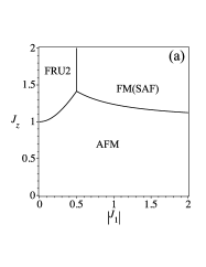
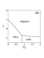
Figure 2: The ground-state phase diagram in the $|J_{1}|$-$J_{z}$ plane for the fixed values of the coupling constants: (a) $J_{x}=1$, $J_{0}=-1$; (b) $J_{x}=1$, $J_{0}=1$.

In figure 2 we illustrate the ground-state phase diagrams in the $|J_{1}|$-$J_{z}$ plane by considering the fixed values of the coupling constants: (a) $J_{x}=1$, $J_{0}=-1$. While the change in sign of the transverse component of the Heisenberg interaction $J_{x}$ is merely responsible for a change of the symmetry of the eigenvectors (23) and (29), the change in character of the Ising inter-leg coupling $J_{0}$ basically influences the overall ground-state phase diagram. In fact, the former case with the antiferromagnetic Ising coupling $J_{0}=-1$ involves just four different ground states: FM, SAF, AFM and FRU2. The phase boundary between FRU2 and FM(SAF) is delimited by the condition $|J_{1}|=1/2$, the phase boundary between FRU2 and AFM is given by $J_{z}=\sqrt{4J_{1}^{2}+J_{x}^{2}}$ and finally, the phase boundary between AFM and FM(SAF) is determined by $J_{z}=J_{0}-2|J_{1}|+\sqrt{4J_{1}^{2}+J_{x}^{2}}$. Meanwhile, figure 2b illustrates the ground-state phase diagram for another particular case with the ferromagnetic Ising inter-leg coupling $J_{0}=1$, which displays the frustrated ground state FRU1 instead of the other frustrated ground state FRU2. The phase boundary between FRU1 and AFM is delimited by $|J_{1}|=\frac{\sqrt{3}}{2}$, whereas the phase boundary between FRU1 and FM (SAF) is given by $J_{z}=|J_{x}|-2|J_{1}|$, and between AFM and FM(SAF) is $J_{z}=J_{0}-2|J_{1}|+\sqrt{4J_{1}^{2}+J_{x}^{2}}$.

III Thermodynamics

To study the thermodynamics of the spin-1/2 Ising-Heisenberg ladder with alternating inter-leg couplings, let us calculate first the partition function given by

$$\mathcal{Z}_{N}=\sum_{\{S\}}\left(\prod_{i=1}^{N}\mathrm{tr}_{i}\mathrm{e}^{-\beta\left(H_{i,i+1}^{XXZ}+H_{i,i+1}^{I}+H_{i,i+1}^{IH}\right)}\right).$$ (32)

Here, $\beta=1/(k_{{\rm B}}T)$, $k_{{\rm B}}$ is being the Boltzmann’s constant, $T$ is the absolute temperature, the symbol $\mathrm{tr}_{i}$ denotes a trace over spin degrees of freedom of the $i$th Heisenberg spin pair, the summation $\sum_{\{S\}}$ runs over all states of the effective Ising spins $S=3/2$. After tracing out the spin degrees of the Heisenberg spins one may employ the usual transfer-matrix approach baxter-book in order to calculate the partition function. The transfer matrix $\boldsymbol{T}=\mathrm{tr}_{i}\Big{(}\mathrm{e}^{-\beta\left(H_{i,i+1}^{XXZ}+H_{i,i+1}^{I}+H_{i,i+1}^{IH}\right)}\Big{)}$ takes the following form

$$\boldsymbol{T}=\left(\begin{array}[]{cccc}w_{1,1}&w_{1,2}&w_{1,2}&w_{1,4}\\ w_{1,2}&w_{2,2}&w_{1,4}v^{-2}&w_{1,2}\\ w_{1,2}&w_{1,4}v^{-2}&w_{2,2}&w_{1,2}\\ w_{1,4}&w_{1,2}&w_{1,2}&w_{1,1}\end{array}\right).$$ (33)

where individual matrix elements are explicitly given by

$$w_{1,1}= vz\left(y^{4}+y^{-4}\right)+\frac{v}{z}\left(x^{2}+x^{-2}\right),$$ (34)

$$w_{1,2}= z\left(y^{2}+y^{-2}\right)+z^{-1}(y_{1}^{2}+y_{1}^{-2}),$$ (35)

$$w_{1,4}= 2vz+\frac{v}{z}\left(x^{2}+x^{-2}\right),$$ (36)

$$w_{2,2}= 2\frac{z}{v}+\frac{1}{vz}\left(y_{2}^{2}+y_{2}^{-2}\right),$$ (37)

with $x=\mathrm{e}^{\beta J_{x}/4}$ , $y=\mathrm{e}^{\beta J_{1}/4}$, $z=\mathrm{e}^{\beta J_{z}/4}$, $v=\mathrm{e}^{\beta J_{0}/4}$, $y_{1}=\mathrm{e}^{\beta\sqrt{J_{x}^{2}+J_{1}^{2}}/4}$, and $y_{2}=\mathrm{e}^{\beta\sqrt{J_{x}^{2}+4J_{1}^{2}}/4}$.

The eigenvalues $\lambda$ of the transfer matrix (33) follow from the solution of eigenvalue problem $\text{det}(\boldsymbol{T}-\lambda)=0$. The determinant drops into a fourth-order polynomial in $\lambda$, which can be further factorized to

$$\left(\lambda-w_{2,2}+\frac{w_{1,4}}{v^{2}}\right)\left(\lambda-w_{1,1}+w_{1,4}\right)\times$$

$$\left(\lambda^{2}-2(p+q)\lambda+4pq-16r^{2}\right) =0.$$ (38)

The coefficients of quadratic polynomial are given by

$$p= 2\left[{\rm e}^{\beta\frac{J_{0}+J_{z}}{4}}{\rm ch}\left(\tfrac{\beta J_{1}}{2}\right)^{2}+{\rm e}^{\beta\frac{J_{0}-J_{z}}{4}}{\rm ch}\left(\tfrac{\beta J_{x}}{2}\right)\right],$$ (39)

$$q= {\rm e}^{\frac{-\beta\left(J_{0}+J_{z}\right)}{4}}\left[{\rm ch}(\tfrac{\beta}{2}\sqrt{J_{x}^{2}+4J_{1}^{2}})+{\rm ch}(\tfrac{\beta J_{x}}{2})\right]+2{\rm e}^{\frac{-\beta\left(J_{0}-J_{z}\right)}{4}},$$ (40)

$$r= {\rm e}^{\beta\frac{J_{z}}{4}}{\rm ch}\left(\tfrac{\beta J_{1}}{2}\right)+{\rm e}^{-\beta\frac{J_{z}}{4}}{\rm ch}\left(\tfrac{\beta}{2}\sqrt{J_{x}^{2}+J_{1}^{2}}\right).$$ (41)

After that, one finds the following explicit form of the transfer-matrix eigenvalues

$$\lambda_{0}= p+q+\sqrt{(p-q)^{2}+16r^{2}},$$ (42)

$$\lambda_{1}= p+q-\sqrt{(p-q)^{2}+16r^{2}},$$ (43)

$$\lambda_{2}= \frac{\left(x^{2}y_{2}^{2}-1\right)\left(y_{2}^{2}-x^{2}\right)}{zx^{2}vy_{2}^{2}},$$ (44)

$$\lambda_{3}= \frac{vz\left(y^{4}-1\right)^{2}}{y^{4}}.$$ (45)

It can be easily seen that the first eigenvalue (42) is always positive and it always represents the largest eigenvalue of the transfer matrix. In the thermodynamic limit $N\to\infty$, the Helmholtz free energy per unit cell is given only by the largest transfer-matrix eigenvalue through

$$f=-\frac{1}{\beta}\ln\left(p+q+\sqrt{(p-q)^{2}+16r^{2}}\right),$$ (46)

where $p$, $q$ and $r$ are given by Eqs. (39)-(41). The basic thermodynamic quantities as the entropy or specific heat can be simply obtained from the Helmholtz free energy using the standard thermodynamic relations.

III.1 Entropy and specific heat

In figure 3(a) we illustrate temperature dependence of the entropy for the fixed values of the coupling constants $J_{0}=-1$, $J_{x}=1$. The choice of the interaction parameters {$J_{1}=0.56$, $J_{z}=1.4$} drives the investigated model close to a triple coexistence point of the phases FM, AFM and FRU2, which lies in figure 2(a) at the coordinates {$J_{1}=0.5$, $J_{z}=\sqrt{2}$}. As one can see, the temperature dependence of the entropy shows a steep increase at low temperature $T\approx 0.01$, which is followed by a gradual temperature variation until another steeper change is reached at the moderate temperature $T\approx 0.2$. Similar behavior can be detected close to the phase boundary of FRU2 and AFM when assuming fixed { $J_{1}=0.4$, $J_{z}=1.23$}, as well as near the phase boundary of FRU2 and FM(SAF) assuming fixed {$J_{1}=1.0$, $J_{z}=1.25$}.

These trends are also reflected in the corresponding thermal variations of the specific heat, which are displayed in figure 3(b). The specific heat evidently shows a pronounced double-peak temperature dependence, whereas the low-temperature peak is relatively high and sharp in a linear scale but it becomes round in a logarithmic scale. Contrary to this, the high-temperature peak is broad both in a linear as well as logarithmic scale. Obviously, the anomalous low-temperature peak appears due to low-lying thermal excitations as all three phases FM, AFM and FRU2 have equal energy at the triple point given by $J_{1}=0.5$ and $J_{z}=\sqrt{2}$.

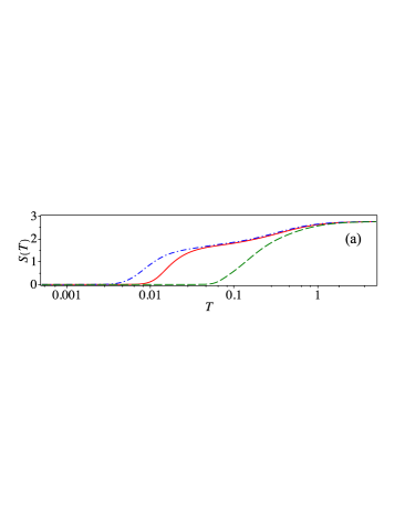
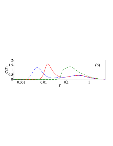
Figure 3: (a) The entropy as a function of the temperature for the fixed values of the coupling constants $J_{0}=-1$ and $J_{x}=1$. The solid line corresponds to a set of the interaction parameters {$J_{1}=0.56$, $J_{z}=1.4$}, the dashed line corresponds to the set { $J_{1}=0.4$, $J_{z}=1.23$} and the dashed-dotted line corresponds to the set {$J_{1}=1.0$, $J_{z}=1.25$}; (b) The corresponding temperature dependence of the specific heat for the same set of the interaction parameters in (a).

In figure 4(a) we display the entropy as a function of temperature for the fixed value of the ferromagnetic Ising inter-leg coupling $J_{0}=1$ and three different sets of the interaction parameters. In all these plots one observes a unusual thermal behavior of the entropy at sufficiently low temperature, where it shows an abrupt but still continuous thermally-induced increase. This sudden increase in the entropy is strongly reminiscent of the entropy jump, which always accompanies a discontinuous (first-order) phase transition. However, the abrupt but still continuous rise of the entropy appears here owing to vigorous thermal excitations from two-fold degenerate AFM ground state towards the macroscopically degenerate FRU1 state. Therefore, the sudden rise of the entropy takes place at the temperature

$$T_{p}=\frac{\sqrt{4J_{1}^{2}+J_{x}^{2}}+J_{z}-|J_{x}|}{2\ln 2},$$ (47)

which can be obtained from a comparison of the Helmholtz free energy of the AFM and FRU1 phases when simply ignoring a thermal change of their internal energies. To provide a deeper insight, we have plotted in figure 4(b) and (c) thermal variations of the specific heat for the same set of parameters as for the entropy. The specific heat exhibits remarkable double-peak temperature dependence with a very sharp and narrow low-temperature maximum. The anomalous specific-heat peak at low temperatures is strongly reminiscent because of its extraordinary height and sharpness to an anomaly accompanying a phase transition, but this peak is finite. The sharp low-temperature peak of the specific heat can be thus identified with the Schottky-type maximum gopal ; karlova , which is caused by intense thermal excitations from the two-fold degenerate ground state AFM towards the macroscopically degenerate excited state FRU1 driven by a high entropy gain. As a matter of fact, the locus of the anomalous peak is in accordance with the condition (47).

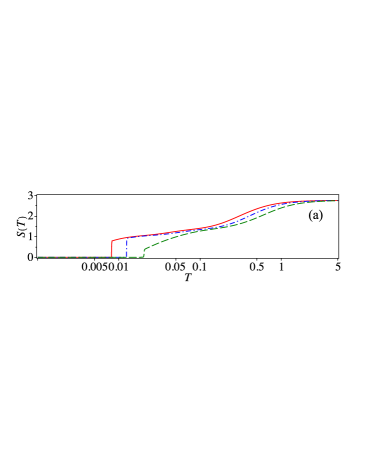
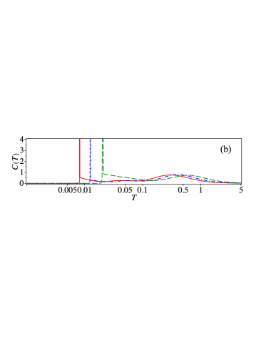
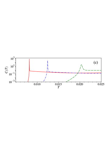
Figure 4: (a) Thermal variations of the entropy for the fixed value of the Ising inter-leg coupling $J_{0}=1$ and three different sets of the interaction parameters. The solid line corresponds to a set of the interaction parameters {$J_{x}=0.5$, $J_{1}=0.724$, $J_{z}=-0.9215$}, the dashed line corresponds to the set {$J_{x}=1$, $J_{1}=0.89$, $J_{z}=-0.75$} and the dashed-dotted line corresponds to the set {$J_{x}=2$, $J_{1}=1.2$, $J_{z}=-0.28$}; (b) The specific heat as a function of the temperature for the same set of parameters; (c) The semi-logarithmic plot of the specific heat in a temperature range, where a sharp low-temperature peak appears.

IV Bipartite entanglement

Another fascinating topic that reserves its own right is a quantum entanglement between the Heisenberg spin pairs. The quantity referred to as the concurrence can be relatively simply adapted to quantify the quantum entanglement between the spin-1/2 Heisenberg pair $\sigma_{a,i}$ and $\sigma_{b,i}$. The concurrence is defined through the reduced density matrix $\rho$ wooters

$$\mathcal{C}(\rho)=\max\{{0,2\Lambda_{max}-\text{{tr}}\left(\sqrt{R}\right)}\},$$ (48)

where

$$R=\rho\sigma^{y}\otimes\sigma^{y}\rho^{*}\sigma^{y}\otimes\sigma^{y}.$$ (49)

Above, $\Lambda_{max}$ is the largest eigenvalue of the matrix $\sqrt{R}$, $\rho^{*}$ represent the complex conjugate of the reduced density matrix $\rho$ and $\sigma^{y}$ is being the usual Pauli matrix. The elements of the reduced density matrix bukman can be expressed in terms of the correlation functions amico . Thus, the concurrence is simply given by

$$\mathcal{C}=\max\{0,4|\langle\sigma_{a}^{x}\sigma_{b}^{x}\rangle|-|\frac{1}{2}+2\langle\sigma_{a}^{z}\sigma_{b}^{z}\rangle|\}.$$ (50)

Two spatial components for the correlation function of the Heisenberg spin pairs can be either obtained from the free energy, or equivalently from the largest transfer-matrix eigenvalue using the following relation

$$\langle\sigma_{a}^{x}\sigma_{b}^{x}\rangle=\frac{1}{2\beta\lambda_{0}}\frac{\partial\lambda_{0}}{\partial J_{x}},\quad\text{and}\quad \langle\sigma_{a}^{z}\sigma_{b}^{z}\rangle=\frac{1}{\beta\lambda_{0}}\frac{\partial\lambda_{0}}{\partial J_{z}}.$$ (51)

Alternatively, the concurrence for the Heisenberg spin pairs can be written as

$$\mathcal{C}=\frac{1}{2\beta\lambda_{0}}\max\{0,4|\frac{\partial\lambda_{0}}{\partial J_{x}}|-|\beta\lambda_{0}+4\frac{\partial\lambda_{0}}{\partial J_{z}}|\}.$$ (52)

IV.1 Quantum entanglement

First, let us take a closer look at the ground-state behavior of the concurrence. It is worthy to mention that the Heisenberg dimers are maximally entangled ($\mathcal{C}=1$) at zero temperature just within the FRU1 ground state. On the other hand, the AFM ground state also shows at zero temperature the quantum entanglement of the Heisenberg dimers when the concurrence depends on a relative strength of the interaction parameters $J_{x}$ and $J_{1}$

$$\mathcal{C}=\frac{|J_{x}|}{\sqrt{4J_{1}^{2}+J_{x}^{2}}}.$$ (53)

Contrary to this, the Heisenberg dimers are fully disentangled ($\mathcal{C}=0$) within the other three classical ground states FM, SAF and FRU2. It can be seen from figure 5 that the zero-temperature variations of the concurrence clearly demonstrate a first-order phase transition from the FRU1 ground state to the AFM ground state through the relevant discontinuity in the concurrence, assuming fixed $J_{0}=-1$ and $J_{z}=-1$. In general, the transverse component $J_{x}$ of the Heisenberg inter-leg coupling enhances the concurrence, which is contrarily suppressed by the Ising intra-leg interaction $J_{1}$.

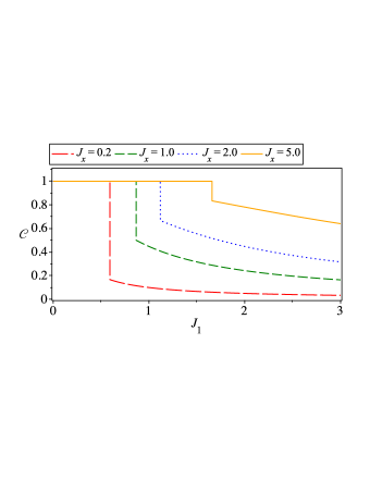
Figure 5: Zero-temperature variations of the concurrence with the Ising intra-leg interaction $J_{1}$ for several values of the transverse component $J_{x}$ of the Heisenberg inter-leg interaction, assuming fixed $J_{0}=-1$ and $J_{z}=-1$.

IV.2 Thermal entanglement

Next, let us discuss thermal entanglement of the Heisenberg dimers at finite temperatures. In figure 6 we have plotted the concurrence as a function of temperature for the set of parameters driving the investigated system towards the AFM ground state. The AFM ground state is entangled albeit not fully, because the concurrence depends according to Eq. (53) on a competition between the coupling constants $J_{x}$ and $J_{1}$. Figure 6 illustrates an influence of the longitudinal component $J_{z}$ of the Heisenberg inter-leg interaction on the concurrence at finite temperature, which is however completely independent thereof at zero temperature. In accordance with this statement, all displayed thermal dependences of the concurrence tend towards the same zero-temperature asymptotic limit given by Eq. (53). On the other hand, it turns out that the concurrence is highly sensitive to the Heisenberg coupling constant $J_{z}$ at higher temperature. Apart from a monotonous decline of the concurrence with the rising temperature, one surprisingly finds more peculiar non-monotonous thermal dependences of the concurrence as shown in figure 6.

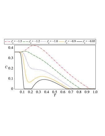
Figure 6: Temperature dependences of the concurrence for the fixed values of the couplings constants $J_{0}=1$, $J_{x}=1$, $J_{1}=1.3$ and several values of the interaction parameter $J_{z}$.

In figure 7, we display one additional plot of the concurrence exactly at and very close to a phase boundary between the AFM and FRU1 ground states by keeping the coupling constants $J_{0}=1$ and $J_{x}=1$ fixed. The dashed-dotted (red) curve corresponds to a coexistence of the AFM and FRU1 ground states, which occurs on assumption that $J_{1}=\sqrt{3}/2$ and $J_{z}=-1$. As one can see, the concurrence starts from its maximum asymptotic value $\mathcal{C}=1$ in this particular case due to an infinite degeneracy of the FRU1 ground states. The other temperature dependences of the concurrence are plotted in figure 7 for $J_{1}=\sqrt{3}/2+0.04$ and different values of $J_{z}$, which fall into a parameter space of the AFM ground state. Owing to this fact, the zero-tempeture limit of the concurrence dramatically falls to $\mathcal{C}\simeq 0.4832$ in accordance with Eq. (53). This sudden change is related to the zero-temperature discontinuity of the concurrence at $J_{1}=\sqrt{3}/2$ provided that the other three coupling constants $J_{0}=1$, $J_{1}=1$ and $J_{z}=-1$ are fixed.

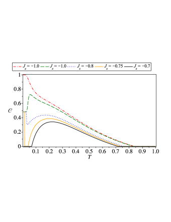
Figure 7: The concurrence as a function of temperature for the fixed values of the interaction parameters $J_{0}=1$ and $J_{x}=1$. The dashed-dotted (red) curve corresponds to a coexistence of the AFM and FRU1 ground states at $J_{1}=\sqrt{3}/2$ and $J_{z}=-1$. The other curves are plotted for $J_{1}=\sqrt{3}/2+0.04$ and different values of $J_{z}$, which all fall into a parameter space of the AFM ground state.

The thermal entanglement within another parameter space, which corresponds to the FRU1 ground state, exhibits standard temperature dependences with a gradual monotonous temperature decline of the concurrence starting from its maximum value $\mathcal{C}=1$ at zero temperature. From this perspective, there is no need to display the standard thermal variations of the concurrence within this parameter region.

IV.3 Threshold temperature

The threshold temperature is one of the most relevant quantities used for a characterization of the thermal entanglement, since it delimits the entangled parameter space from the disentangled one. The threshold temperature can be simply attained from Eq. (52) when letting the concurrence tend to zero from a non-zero side. Accordingly, the threshold temperature can be obtained from a numerical solution of the following transcendent (with respect to temperature) equation

$$4|\frac{\partial\lambda_{0}}{\partial J_{x}}|=|\beta\lambda_{0}+4\frac{\partial\lambda_{0}}{\partial J_{z}}|.$$ (54)

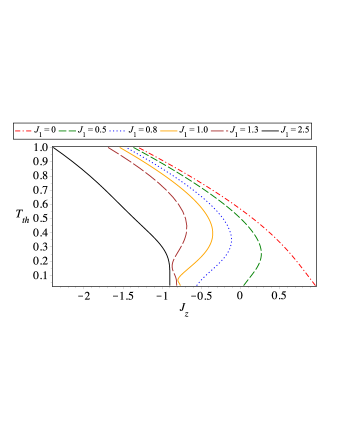
Figure 8: The threshold temperature $T_{th}$ against the coupling constant $J_{z}$ for the fixed values of the interaction parameters $J_{0}=1$, $J_{x}=1$ and several values of the Ising intra-leg interaction $J_{1}$.

The threshold temperature $T_{th}$ is plotted in figure 8 against the longitudinal component $J_{z}$ of the Heisenberg inter-leg coupling by considering the fixed interaction parameters $J_{x}=1$, $J_{0}=1$ and varying a strength of the Ising intra-leg coupling $J_{1}$. The limiting case $J_{1}=0$ corresponds a set of non-interacting Ising and Heisenberg dimers and hence, the threshold temperature exactly coincides with that one of the spin-1/2 Heisenberg dimer that monotonically decreases with $J_{z}$ until zero temperature is reached at the isotropic Heisenberg point $J_{x}=J_{z}=1$. The relevant behavior of the threshold temperature becomes much more complex for $J_{1}>0$, because it may show a peculiar reentrant behavior when the entangled region re-appears at temperatures above the disentangled region. The reentrant behavior of the concurrence can be clearly seen for instance in figure 6 for the parameter set $J_{0}=1$, $J_{x}=1$, $J_{z}=-0.85$ and $J_{1}=1.3$ (black line with three threshold temperatures). Apart from the triple reentrance, the threshold temperature may also show double reentrance (e.g. for $J_{1}=0.5$ in figure 8) when the thermal entanglement emerges above the disentangled ground state. It is worthy to notice that the reentrant phenomenon disappear for the Ising intra-leg couplings stronger than $J_{1}\gtrsim 2.5$.

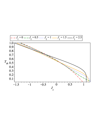
Figure 9: The threshold temperature $T_{th}$ against the coupling constant $J_{z}$ for the fixed values of the interaction parameters $J_{0}=-1$, $J_{x}=1$ and several values of the Ising intra-leg interaction $J_{1}$.

Last but not least, the threshold temperature $T_{th}$ is displayed in figure 9 as a function of the coupling constant $J_{z}$ for the fixed values of the interaction parameters $J_{0}=-1$, $J_{x}=1$ and several values of the Ising intra-leg coupling $J_{1}$. The trivial case $J_{1}=0$ shown by the dashed-dotted (red) line, which corresponds to the isolated spin-1/2 Heisenberg dimers, repeatedly serve as a landmark to compare with. As soon as the Ising intra-leg coupling $J_{1}$ is turned on, the threshold temperature reaches zero at higher values of the coupling constant $J_{z}$, but afterwards it recovers the zero-temperature asymptotic value $J_{z}\rightarrow 1$ for strong enough Ising intra-leg couplings $J_{1}\gg 1$.

V Conclusion

In the present work, we have exactly solved the spin-1/2 Ising-Heisenberg ladder accounting for regularly alternating Ising and Heisenberg inter-leg couplings in addition to the Ising intra-leg interaction. It has been evidenced that the investigated model is equivalent to the mixed spin-(3/2,1/2) Ising-Heisenberg diamond chain with the nodal Ising spin $S=3/2$ and the interstitial spin-1/2 Heisenberg dimers, which was exactly treated by means of the transfer-matrix method. Using this rigorous procedure, we have found that the ground-state phase diagram involves in total five different ground states: ferromagnetic, antiferromagnetic, super-antiferromagnetic and two types of highly degenerated (frustrated) ground-state manifolds. The antiferromagnetic and one of frustrated ground states are quantum in character as exemplified by the quantum and thermal entanglement of the Heisenberg dimers. In addition, the concurrence as a measure of the thermal entanglement may exhibit a striking reentrant behavior.

We have also exactly calculated the entropy and specific heat, which may display under certain conditions anomalous thermal dependences. The entropy may exhibit at sufficiently low temperatures an abrupt but still continuous rise, which gives rise to an extraordinary high and sharp specific-heat maximum. The relevant temperature dependences of the entropy and specific heat thus mimic in many respects a temperature-driven phase transition, but they should not be confused as signatures of it. The anomalous thermal behavior of the entropy and specific heat occurs in the present model due to a high entropy gain, which originates from vigorous thermal excitations between the two-fold degenerate ground state and the highly degenerate excited state close enough in energy. The model under investigated thus falls into a prominent class of the exactly solved systems with such an intriguing magnetic behavior gali ; alec .

References

- (1) P. Fulde, Electron Correlations in Molecules and Solids (Springer, Berlin, 1995).
- (2) P. Fazekas, Lecture Notes on Electron Correlation and Magnetism (World Scientific, Singapore, 1999).
- (3) J.S. Bell, Speakable and Unspeakable in Quantum Mechanics (Cambridge University Press, Cambridge, 1987).
- (4) M.A. Nielsen, I.L. Chuang, Quantum Computation and Quantum Information (Cambridge University Press, Cambridge, 2000).
- (5) L. Amico, R. Fazio, A. Osterloh, V. Vedral, Rev. Mod. Phys. 80, 517 (2008).
- (6) M.T. Batchelor, X.W. Guan, N. Oelkers, Z. Tsuboi, Adv. Phys. 56, 465 (2007).
- (7) B. Chiari, O. Piovesana, T. Tarantelli, P.F. Zanazzi, Inorg. Chem. 29, 1172 (1990).
- (8) Z. Hiroi, M. Azuma, M. Takano, and Y. Bando, J. Solid State Chem. 95, 230 (1991).
- (9) R. D. Willett, C. Galeriu, C. P. Landee, M. M. Turnbull, B. Twamley, Inorg. Chem. 43, 3804 (2004).
- (10) M. Onoda, N. Nishiguci, J. Solid State Chem. 127, 359 (1996).
- (11) T. Barnes, J. Riera, Phys. Rev. B 50, 6817 (1994).
- (12) G. Simutis, S. Gvasaliya, F. Xiao, C. P. Landee, A. Zheludev, Phys. Rev. B 93, 094412 (2016).
- (13) F. Amiri, G. Sun, H.-J. Mikeska, T. Vekua, Phys. Rev. B 92, 184421 (2015)
- (14) J. Oitmaa, R. R. P. Singh, Z. Weihong, Phys. Rev. B 54, 1009 (1996).
- (15) G.I. Japaridze, E. Pogosyan, J. Phys.: Condens. Matter, 18, 9297 (2006).
- (16) F. B. Ramos, J. C. Xavier, Phys. Rev. B 89 094424 (2014).
- (17) T. Verkholyak, J. Strečka, Condens. Matter Phys. 16, 13601 (2013).
- (18) T. Verkholyak, J. Strečka, J. Phys. A: Math. Theor. 45, 305001 (2012).
- (19) J. Strečka, O. Rojas, T. Verkholyak, M. L. Lyra, Rev. E 89, 022143 (2014).
- (20) O. Rojas, J. Strečka, M.L. Lyra, Phys. Lett. A 377, 920 (2013).
- (21) W. Van den Heuvel, L. F. Chibotaru, Phys. Rev. B 82, 174436 (2010).
- (22) S. Sahoo, J. P. Sutter, S. Ramasesha, J. Stat. Phys. 147, 181 (2012).
- (23) S. Bellucci, V. Ohanyan, O. Rojas, EPL 105, 47012 (2014).
- (24) J. Strečka, M. Hagiwara, Y. Han, T. Kida, Z. Honda, M. Ikeda, Condens. Matter Phys. 15, 43002 (2012).
- (25) J. S. Valverde, O. Rojas, S. M. de Souza, J. Phys.: Condens. Matter, 20, 345208 (2008).
- (26) V. Ohanyan, Condens. Matter Phys. 12, 343 (2009).
- (27) D. Antonosyan, S. Bellucci, V. Ohanyan, Phys. Rev. B 79, 014432 (2009).
- (28) L. Čanová, J. Strečka, T. Lučivjanský, Condens. Matter Phys. 12, 353 (2009).
- (29) O. Rojas, S. M. de Souza, V. Ohanyan, M. Khurshudyan, Phys. Rev. B 83, 094430 (2011).
- (30) N. Ananikian, L. Ananikyan, L. Chakmakhyan, O. Rojas, J. Phys.: Condens. Matter 24, 256001 (2012).
- (31) J. Strečka, M. Jasčur, M. Hagiwara, Y. Narumi, K. Kindo and K. Minami, Phys. Rev. B, 72, 024459. (2005).
- (32) O. Rojas, M. Rojas, N. S. Ananikian, S. M. de Souza, Phys. Rev. A 86, 042330 (2012).
- (33) V. Ohanyan, O. Rojas, J. Strečka, S. Bellucci, Phys. Rev. B 92, 214423 (2015).
- (34) O. Rojas, S. M. de Souza, Eur. Phys. J. B 85 (2012) 170. N. Sh. Izmailian, O. Rojas, S. M. de Souza, Physica A 391, 552 (2012).
- (35) R.J. Baxter, Exactly Solved Models in Statistical Mechanics, (Academic Press, New York, 1982).
- (36) W. K. Wootters, Phys. Rev. Lett. 80, 2245 (1998).
- (37) D. J. Bukman, G. An, and J. M. J. van Leeuwen, Phys. Rev. B 43, 13352 (1991).
- (38) L. Amico, A. Osterloh, F. Plastina, R. Fazio, G. M. Palma, Phys. Rev. A 69, 022304 (2004).
- (39) E.S.R. Gopal, Specific Heats at Low Temperatures (Heywood Books, London, 1966, pp.102-105).
- (40) K. Karlová, J. Strečka, T. Madaras, Physica B 488, 49 (2016).
- (41) L. Gálisová, J. Strečka, Phys. Rev. E 91, 022134 (2015).
- (42) J. Strečka, R.C. Alécio, M.L. Lyra, O. Rojas, J. Magn. Magn. Mater. 409, 124 (2016).