Numerical analysis of homogeneous and inhomogeneous intermittent search strategies

Abstract

A random search is a stochastic process representing the random motion of a particle (denoted as the searcher) that is terminated when it reaches (detects) a target particle or area the first time. In intermittent search the random motion alternates between two or more motility modes, one of which is non-detecting. An example is the slow diffusive motion as the detecting mode and fast, directed ballistic motion as the non-detecting mode, which can lead to much faster detection than a purely diffusive search. The transition rate between the diffusive and the ballistic mode (and back) together with the probability distribution of directions for the ballistic motion defines a search strategy. If these transition rates and/or probability distributions depend on the spatial coordinates within the search domain it is a spatially inhomogeneous search strategy, if both are constant, it is a homogeneous one. Here we study the efficiency, measured in terms of the mean first-passage time, of spatially homogeneous and inhomogeneous search strategies for three paradigmatic search problems: 1) the narrow escape problem, where the searcher has to find a small area on the boundary of the search domain, 2) reaction kinetics, which involves the detection of an immobile target in the interior of a search domain, and 3) the reaction-escape problem, where the searcher first needs to find a diffusive target before it can escape through a narrow region on the boundary. Using families of spatially inhomogeneous search strategies, partially motivated by the spatial organization of the cytoskeleton in living cells with a centrosome, we show that they can be made almost always more efficient than homogeneous strategies.

I Introduction

The successful usage of efficient search strategies is one of the most important needs in biology and human behavior. It can be observed on all length scales of life and in all kinds of complexity. Just to mention a few examples, humans use them for pattern recognition Najemnik2008 . Predators apply certain strategies for hunting their moving prey Humphries2010 . Ants use special techniques to find each other after being separated while being on a tandem run Franks2010 . Some eukaryotic cells improve their chance to find a target by performing random walks with characteristic persistent time and persistent lengths, even in the absence of external signals Li2008 . And there are many more observed examples in biological literature.
Although all these examples are quite different and seem to have nothing in common, they can commonly be described by first-passage processes Redner2001book , which are stochastic processes that end if a certain event happens for the first time $t_{f}$. The probability density $\rho_{f}$ for the time $t_{f}$ contains all temporal information about the efficiency of the search strategy. In Mattos2012 it is shown, that one sometimes has to be careful with the reduction of this information to only one value, the so called mean first-passage time (MFPT)

$$T=\braket{\,t_{f}\,}=\int_{0}^{\infty}t\;\rho_{f}(t)\;dt\;.$$

Nevertheless, this is in most cases the only property which is used to classify the efficiency of the search strategy. Apart from the obvious reason of simplification for comparison, there is a second reason for this reduction: Often it is very hard or even impossible to calculate the whole first-passage time density function $\rho_{f}(t)$ as a function of the initial conditions, but it is much easier to solve the time-independent differential equation system for its first moment, which is derived with the help of corresponding backward equations Risken1996book ; Redner2001book .
The MFPT $T$ is a function of the tunable and the non-tunable parameters of the stochastic first-passage process. Typical tunable parameters are for example the persistence length in random walks Tejedor2012 , the desorption rate in surface mediated diffusion Benichou2010 ; Calandre2014 or the resetting rate in random motion with stochastic resetting Evans2011 ; Kusmierz2014 . Typical non-tunable parameters of the search problem are for example the target size, the detection rate, the size and shape of the searching domain and constants of motion (velocity, diffusivity). A complete set of tunable parameters defines a search strategy for the problem which is defined via the non-tunable parameters. Hence, the best strategy is the set of tunable parameters which minimizes the MFPT $T$.

A frequently used way of modeling real search is a so called intermittent search Benichou2005 ; Benichou2005a ; Benichou2007 ; Benichou2011 ; Loverdo2008 ; Bressloff2009 ; Loverdo2009 ; Smith2001 ; Bressloff2012 . The searcher switches between phases of fast directed ballistic motion, during which it cannot recognize a target and phases of slow diffusion for detecting a target.

For a given size and shape of the search domain and the target, the efficiency, i.e. the MFPT $T$, of an intermittent search still depends on a number of parameters. Since increasing the diffusion constant for the diffusive mode or increasing the velocity modulus $v$ for the ballistic mode always decreases the MFPT, even if done only locally, both are assumed to be fixed in the following. Then the MFPT $T$ is a function of the switching rates between both motility modes and a functional of distribution of the directions into which the searcher moves after a switch to the ballistic mode. If the searcher does not have a knowledge about his position in the search domain and the search domain is homogeneous such that at no position in the search domain certain directions for ballistic motion are preferred the directional distribution can be assumed to be uniform over all solid angles - as was done in Benichou2005 ; Benichou2005a ; Benichou2007 ; Benichou2011 ; Loverdo2008 ; Loverdo2009 . This we denote as a spatially homogeneous (and isotropic) intermittent search strategy.
If on the other hand ballistic motion is only possible along predefined tracks, like in molecular motor assisted intracellular transport along the filaments of the cytoskeleton Alberts2014book , or in cases the searcher utilizes any other transport network, the directional distribution for the ballistic motion should be described by a spatially inhomogeneous direction distribution, which then must represent the spatial organization of the tracks. Also in cases when the searcher does have knowledge about its position in the search domain and about its shape it might be more efficient to move in certain regions of the search domain preferentially into other directions than in other regions. An intermittent search strategy with a spatially varying direction distribution we denote as a spatially inhomogeneous (and non-isotropic) search strategy. In a recent letter schwarz2016 we introduced the concept of spatially inhomogeneous intermittent search strategies and we presented results that showed that their optimum is in general more efficient than the optimum of homogeneous search strategies. In this paper we elaborate these and more results in detail, explain the computational techniques and show all computations explicitly.

Thus the goal of this paper is to compare the efficiency of spatially homogeneous and inhomogeneous search strategies in spherical domains by determining, numerically, the optimal parameter for different setups: 1) the narrow escape problem , where a searcher has to find a small region on the boundary of the search area, 2) the reaction kinetics enhancement by ballistic motion, where the searcher has to find a immobile target particle within the search domain, and 3) the reaction-escape problem, which combines 1 and 2 such that a searcher has to find a mobile target particle first before it can escape through a narrow region on the boundary of the search domain. The latter example is motivated by a transport process within T-cells attached to a target cell that it is supposed to kill: vesicles loaded with cytotoxic proteins first have to attach to another vesicle containing receptor proteins before they can dock at the immunological synapse, a small region on the cell membrane in contact with the target cell, and release their content there.

Since determining the optimum of the MFPT as a functional of a space and angle dependent direction distribution is not feasible we confine ourselves to two different families of direction distributions. The first (one-parameter) family is specially designed for solving the narrow escape problem efficiently and only investigated in that scenario. The second (two-parameter) family is inspired by the spatial organization of the cytoskeleton of spherical cells with a centrosome. It will be studied for all the three scenarios.

In order to compare the gain of efficiency for different situations, we introduce the dimensionless time

$$\mathbb{T}=\frac{T}{T_{\text{diff}}}\;,$$ (1)

which is the MFPT $T$ of the intermittent search strategy normalized by the MFPT $T_{\text{diff}}$ for the purely diffusive searcher. Hence, for $\mathbb{T}<1$ an intermittent searcher is more efficient and for $\mathbb{T}>1$ a purely diffusive search is faster on average.

The paper is organized as follows: Section II introduces our model of intermittent search in the general case with space and time dependent transition rates. It explains the meaning of the occurring parameters exemplarily in the context of intracellular transport. In almost all cases, it is not possible to solve the differential equation system of the model in a straight forward way via finite element method (FEM).
In consequence, section III introduces the Green’s function method, which is used to solve the model stochastically.
Section IV faces the classical narrow escape problem, meaning, a particle looks for a certain region at the boundary. For the purely diffusive scenario the scaling of the MFPT as a function of the size and the position of the target area is understood for quite a large range of problems Krapivsky1996a ; Redner2001book ; Benichou2005b ; Singer2006a ; Singer2006b ; Singer2006c ; Schuss2007 ; Schuss2012 ; Benichou2008 ; Chevalier2011 ; Cheviakov2012 . Even in the absence of analytic or asymptotic expressions, the purely diffusive MFPT problem can be solved fast and easily via FEM calculations. For spatial dimensions $d>1$ this is in most cases not possible for the master equation system of intermittent search (Eqs. (2)-(3)) due to the integro type of the partial differential equation. As far as we know, there are no studies on the intermittent search narrow escape problem in a sphere available. Hence, we start the numeric study of this problem in the case of a homogeneous velocity direction distribution. Afterwards we modify the velocity direction distribution to show, that there are more efficient strategies than a homogeneous one.
Section V asks for the best search strategy for a target located within the sphere. In the case of a homogeneously distributed velocity direction and a target which is centered in the middle of the sphere, there are studies on this problem Benichou2011 ; Loverdo2008 ; Loverdo2009 . We numerically confirm their results, including the very weak dependence of the MFPT on the transition rate $\gamma$ from diffusive to ballistic motion, but disprove their optimality assumption for $\gamma$. Furthermore, we study less homogeneous cases, for which there are no MFPT expressions available up to now.
Section VI finally faces a reaction-escape problem for two particles, i.e an intermittent searching predator-particle is looking for a mobile prey-particle. After having found the prey, the particle-complex has to find a small escape area at the boundary. Again, there are already some results for purely diffusive predators in different domains Redner2001book ; Krapivsky1996 ; Redner1999 , but not for intermittent searching ones in a spherical domain.
Finally, appendix A introduces exact and very fast methods to sample the later defined probability densities of the algorithm of section III .

II The model

Intermittent search is generally based on (at least) two different phases for a searcher Benichou2011 . On the one hand, there is a searching phase of slow (or none) motion, in which the searcher is able to detect a target. On the other hand, there is a relocation phase of directed fast motion without the ability of target detection. Commonly, and also in our case, the searching phase is modeled by pure diffusion with diffusivity $D$. The probability density for being in the diffusive state at position $\mathbf{r}\in V$ at time $t$ will be called $P_{0}(\mathbf{r},t)$ in the following, where $V\subset\mathbbm{R}^{d}$ denotes the search volume of the particle. The relocation phase is modeled by straight ballistic motion. The probability density for being in the ballistic state at position $\mathbf{r}\in V$ at time $t$ and moving with velocity $\mathbf{v}_{\Omega}=v\cdot\mathbf{e}_{\Omega}$ is denoted $P_{\Omega}(\mathbf{r},t)$ in the following, where $\mathbf{e}_{\Omega}$ is the unity vector in direction of the solid angle $\Omega$.

In intracellular transport vesicles (proteins, organelles) switch between diffusion within the cytosol and almost ballistic motion by molecular motor assisted movement along cytoskeleton filaments. The density of these filaments in direction of the solid angle $\Omega$ is generally very inhomogeneous in space: for instance in cells with a centrosome microtubules emanate radially from the centrosome towards the cell periphery, where the actin cortex, a thin sheet of actin filaments underneath the cell membrane, provides transport in random directions. Sometimes the filament density even varies over time (for instance during cell polarization). In consequence, the likelihood of a switch between the two phases and the choice of the ballistic direction $\mathbf{e}_{\Omega}$ generally depends on the position of the searcher. Formally we describe a spatially varying distribution of directions by the density $\rho_{\Omega}(\mathbf{r},t)$. It is proportional to the rate of a switch from diffusive to ballistic motion in direction $\Omega$ at position $\mathbf{r}$ at time $t$. In the context of intracellular transport it can be interpreted as the filament density of the cytoskeleton in direction $\Omega$.

The master equation system of our model for one searching particle is given by the Fokker-Planck equation system:

$$\frac{\partial}{\partial t}P_{0}(\mathbf{r},t) = D\Delta P_{0}(\mathbf{r},t)-\left[\gamma\,\int d\Omega\,\rho_{\Omega}(\mathbf{r},t)\right]\,P_{0}(\mathbf{r},t)$$ (2)

$$+\gamma^{\prime}\int d\Omega\,P_{\Omega}(\mathbf{r},t)$$

$$\frac{\partial}{\partial t}P_{\Omega}(\mathbf{r},t) = -\nabla\cdot({\bf v}_{\Omega}P_{\Omega}(\mathbf{r},t))+\gamma\,\rho_{\Omega}(\mathbf{r},t)P_{0}(\mathbf{r},t)$$ (3)

$$-\gamma^{\prime}P_{\Omega}(\mathbf{r},t)\;,$$

where $\gamma$ and $\gamma^{\prime}$ are transition rates from diffusive to ballistic motion and vice versa. In the context of modeling intracellular transport they are the attachment and detachment rates (from cytoskeleton filaments).
In consequence, the diffusing searcher experiences a total annihilation rate

$$k(\mathbf{r},t)=\gamma\int d\Omega\,\rho_{\Omega}(\mathbf{r},t)\;,$$ (4)

with which it is transformed into a ballistically moving particle with a randomly chosen direction $\Omega$ (and velocity ${\bf v}_{\Omega}$) with probability

$$\rho_{\mathbf{v}}(\Omega|\mathbf{r},t)=\frac{\rho_{\Omega}(\mathbf{r},t)}{\int\rho_{\Omega^{\prime}}(\mathbf{r},t)d\Omega^{\prime}}\;.$$ (5)

A ballistically moving particle switches back to diffusive motion with rate $\gamma^{\prime}$.

Within this article, a target shall always be detected immediately, when the diffusive searcher reaches the target area for the first time (in reaction kinetics this means reaction upon contact). One could also consider detection or reaction with a finite rate $k_{\text{det}}$ within the target area Benichou2011 . But we restrict ourselves to the case $k_{\text{det}}\rightarrow\infty$, i.e. target detection is always modeled via the boundary condition

$$P_{0}({\bf r},t)=0\;\quad\forall\;\mathbf{r}\in A\;,$$ (6)

where either $A\subset V$ is the detection area within $V$ or $A\subset\partial V$ is the detection area at the surface of $V$ (narrow escape problem).

In section VI, we consider the problem of two moving particle, which will react immediately if their distance becomes smaller than a certain value. Hence their probability distributions are not independent and the solution does not factorize. Consequently, the master equation system depends on $6$ spatial coordinates and $4$ coordinates for $\Omega$. As the exact notation of this master equation system and the corresponding boundary conditions is very lengthy but straightforward, we will skip it here.

Apart from the initial conditions $P_{0}({\bf r},t=0)=\delta(\bf r-\bf r_{0})$, $P_{\Omega}({\bf r},t)=0$ the equation system is augmented by boundary conditions at the boundary $\partial V\setminus A$ for $P_{0}({\bf r},t)$ and boundary conditions at $\partial V$ for $P_{\Omega}({\bf r},t)$. Two different boundary conditions, in the following called BB (Ballistic-Ballistic) and BD (Ballistic-Diffusive), will be used within the studies of this article.

BB boundary condition

For BB boundary conditions we assume that a ballistically moving particle hitting the boundary is simply reflected and stays in the ballistic mode, no matter whether this happens at the target area or not (i.e. the target is not detected then). A particle in the diffusive mode is reflected at every point of the boundary $\partial V$ , which does not belong to the target area and stays in the diffusive mode. Fig. 1a visualizes the BB condition in a sketch. Formally this boundary conditions are described by

$$\frac{\partial}{\partial\bf{n}_{\bf{r}}}P_{0}({\bf r},t) = 0\quad\quad\forall\;\mathbf{r}\in\partial V\setminus A$$

$$P_{\Omega}({\bf r},t) = P_{\Omega_{\text{refl}}}({\bf r},t)\quad\quad\forall\;\mathbf{r}\in\partial V\;,$$ (7)

where ${\bf{n}_{\bf{r}}}$ denotes the outward pointing unity vector perpendicular to the boundary at position $\mathbf{r}$ and $\Omega_{\text{refl}}$ denotes the solid angle which belongs to the reflection of $\mathbf{e}_{\Omega}$ at the surface position $\mathbf{r}$.

BD boundary condition

For BD boundary conditions we assume that a ballistically moving particle hitting the boundary switches to the diffusive motion. If this part of the boundary belongs to the target area, the particle is immediately detected. A particle in the diffusive mode is reflected at every point of the boundary $\partial V$, which does not belong to the target area and stays in the diffusive mode. Fig. 1b visualizes the BD condition in a sketch. Formally this boundary conditions are described by

$$D\frac{\partial}{\partial\bf{n}_{\bf{r}}}P_{0}({\bf r},t) = \int d\Omega\,\left({{\bf v}_{\Omega}P_{\Omega}({\bf r},t)}\right)\cdot\bf{n}_{\bf{r}}\quad\forall\;\mathbf{r}\in\partial V\setminus A$$

$$P_{\Omega}({\bf r},t) = 0\quad\quad\forall\;{\bf r}\in\partial V,\;\Omega\;|\;{\bf{n}_{\bf{r}}}\cdot{\bf e}_{\Omega}<0\;.$$ (8)

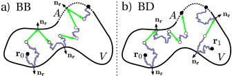
Figure 1: Sketch of boundary conditions in a search volume $V$ with escape area $A$ (dotted line). Grey wiggly lines represent diffusive motion, green lines ballistic motion. a) BB: a ballistically moving particle is reflected at the boundary and stays in the ballistic mode, i.e $A$ is only detected if it is reached diffusively. b) BD: a ballistically moving particle switches to diffusion at the boundary, i.e $A$ will be detected if it reaches $A$ ballistically (trajectory, starting at $\tilde{\bf{r}}_{0}$) or diffusively (trajectory, starting at $\tilde{\bf{r}}_{1}$).

Nondimensionalisation

In order to reduce the number of parameters to a minimal independent set, characteristic length- and time-scales where chosen by introducing the dimensionless spatial and temporal coordinates

$$\tilde{\mathbf{r}}=\frac{1}{R}\mathbf{r}\text{ and }\tilde{t}=\frac{v}{R}t.$$ (9)

In consequence, Eqs. (2) and (3) are always solved in the unit sphere and look the following way:

$$\frac{\partial}{\partial\tilde{t}}P_{0} = \tilde{D}\tilde{\Delta}P_{0}-\tilde{\gamma}\left[\int\rho_{\Omega}(\tilde{\mathbf{r}},t)d\Omega\right]P_{0}+\tilde{\gamma}^{\prime}\int d\Omega\,P_{\Omega}\hskip 14.22636pt$$ (10)

$$\frac{\partial}{\partial\tilde{t}}P_{\Omega} = -\mathbf{e}_{\Omega}\cdot\left(\tilde{\nabla}P_{\Omega}\right)+\tilde{\gamma}\,\rho_{\Omega}(\tilde{\mathbf{r}},t)P_{0}-\tilde{\gamma}^{\prime}P_{\Omega}\;,$$ (11)

with

$$\tilde{D}=\frac{D}{vR},\tilde{\gamma}=\frac{R}{v}\gamma\text{ and }\tilde{\gamma}^{\prime}=\frac{R}{v}\gamma^{\prime}\;.$$ (12)

Apart from the sphere radius $R$, the absolute value of the velocity also vanished in the dimensionless coordinates, as $\tilde{v}=1$ holds. Furthermore, $\mathbb{T}$ is not changed by the dimensionless units, i.e. $\mathbb{T}=T/T_{\text{diff}}=\tilde{T}/\tilde{T}_{\text{diff}}$.

Models for the direction distribution $\rho_{\mathbf{v}}(\Omega|\tilde{\mathbf{r}},\tilde{t})$

Eq. (4) introduced the total transition rate $k(\mathbf{r},t)$ for a switch from diffusive to ballistic motion at position $\mathbf{r}$ at time $t$. Although it is numerically possible to handle this most general scenario (Algorithm 1 in section III) this rate will be constant in time and space in the investigated models, i.e. without further loss of generality we set $\int\rho_{\Omega}(\tilde{\mathbf{r}},\tilde{t})d\Omega=1$ and in consequence Eq. (5) simplifies to

$$\rho_{\mathbf{v}}(\Omega|\tilde{\mathbf{r}},\tilde{t})=\rho_{\Omega}(\tilde{\mathbf{r}},\tilde{t})\;.$$ (13)

Within the studies of this paper, two different families of time-independent inhomogeneous distributions $\rho_{\mathbf{v}}(\Omega|\tilde{\mathbf{r}})$ will be compared to the homogeneous distribution

$$\rho_{\text{hom}}\left({\Omega}\right)=\frac{1}{4\pi}\;.$$ (14)

Both will be rotational symmetric, i.e. $\rho_{\mathbf{v}}(\Omega|\tilde{\mathbf{r}})$ depends only on the radius $\tilde{r}=||\tilde{\mathbf{r}}||$ and the angle

$$\alpha(\tilde{\mathbf{r}},\mathbf{e}_{\Omega})=\text{arcos}\left(\frac{\tilde{\mathbf{r}}\cdot\mathbf{e}_{\Omega}}{||\tilde{\mathbf{r}}||}\right)$$ (15)

between the vectors $\tilde{\mathbf{r}}$ and $\mathbf{e}_{\Omega}$.
This symmetry also holds for the homogeneous case of $\rho_{\text{hom}}\left({\Omega}\right)$, where the probability density for the angle $\alpha\in[0;\pi]$ is independent of $\tilde{\mathbf{r}}$ and given by

$$\rho^{\alpha}_{\text{hom}}(\alpha)=\int_{0}^{2\pi}d\varphi\;\frac{1}{4\pi}\sin(\alpha)=\frac{1}{2}\sin(\alpha)\;.$$ (16)

varying Gaussian distribution

The distribution for the angle $\alpha$ (Eq. (15)) , introduced now, will only be applied to the narrow escape problem. The principle idea is to find the probability density $\rho^{\alpha}\left({\alpha|\tilde{r}}\right)$, which minimizes the MFPT of the narrow escape problem. Mathematically, this is a variational problem. In consequence, a numeric solution requires an apriori assumption for a class of density functions, which is motivated now:
If the particle is close to the center of the simulation sphere, a mainly radially outward pointing velocity direction is for sure the best strategy, as it is the fastest way to reach the sphere’s boundary. At the boundary this distribution is not optimal any more, as there is no velocity component in parallel to the boundary. Without this parallel component, the searcher gets stuck at a relatively small part of the boundary.
In consequence, the spread of the distribution should increase with $\tilde{r}$. Following this argumentation, the gaussian-like probability density $\rho^{\alpha}_{x}\left({\alpha|\tilde{r}}\right)$, illustrated in Fig. 2, was chosen for our simulations:

$$\rho^{\alpha}_{x}\left({\alpha|\tilde{r}}\right)=2\pi\sin(\alpha)\,N\big{(}\sigma\left({x,\tilde{r}}\right)\big{)}\,\exp\left({\frac{-\big{(}\cos(\alpha)-1\big{)}^{2}}{2\left[\sigma\left({x,\tilde{r}}\right)\right]^{2}}}\right)\,,$$ (17)

where

$$\sigma\left({x,\tilde{r}}\right) = \sqrt{\frac{x}{1-x}}\tilde{r}$$ (18)

denotes the spreading of the gaussian and

$$N(\sigma) = \frac{1}{\pi\sigma\sqrt{2\pi}\text{erf}\left({\frac{\sqrt{2}}{\sigma}}\right)}$$ (19)

is the normalization of the distribution.

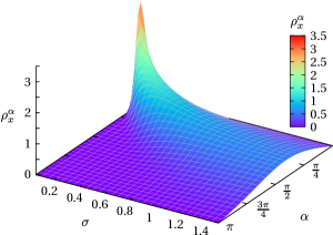
Figure 2: The class of probability densities $\rho^{\alpha}_{x}$ (Eq. (17)) as a function of the variable $\alpha$ and the spreading parameter $\sigma\left({x,\tilde{r}}\right)$.

The class parameter $x\in\;]0;1[$ controls the speed of the increase of the distribution spreading. For $x\rightarrow 0^{+}$, the velocity direction points radially outwards for all $\tilde{r}\in[0;1]$ as $\sigma\left({x,\tilde{r}}\right)$ tends to zero. The spread (Eq. (18)) increases monotonically in $x$ and in $\tilde{r}$. For $x\rightarrow 1^{-}$, we are dealing with the totally homogeneous velocity direction distribution $\rho^{\alpha}_{\text{hom}}(\alpha)$.

radial-peripheral distribution

The second investigated distribution is inspired by the spatial organization of the cytoskeleton of spherical cells with a centrosome and was introduced in schwarz2016 , see Fig. 3a for a sketch. It contains two parameters:

$$\rho_{p,\tilde{\Delta}}^{\alpha}(\alpha|\tilde{r})=\left\{\begin{array}[]{ccc}p\,\delta(\alpha)+(1-p)\,\delta(\alpha-\pi)&,&0<\tilde{r}<1-\tilde{\Delta}\\ \rho^{\alpha}_{\text{hom}}(\alpha)&,&1-\tilde{\Delta}<\tilde{r}<1\end{array}\right..$$ (22)

The parameter $p\in[0;1]$ is the probability to move radially outwards, and $1-p$ the probability to move inwards inside the inner spherical region with radius $1-\tilde{\Delta}$. $\tilde{\Delta}$ represents the width of the outer shell in which the homogeneous strategy is applied, hence $\tilde{\Delta}=1$ represents the totally homogeneous searching strategy. A ballistically moving particle switches to the diffusive state when it reaches the radius $\tilde{r}=0$ and $\tilde{r}=1-\tilde{\Delta}$. The distribution $\rho_{p,\tilde{\Delta}}^{\alpha}$ will only be investigated for the boundary condition BD. A sketch of the resulting stochastic processes is given in Fig. 3b.

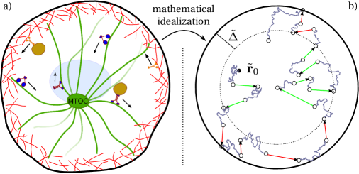
Figure 3: a) The cytoskeleton transport network of a spherical cell with a centrosome: Microtubules (green lines), emanating from the MTOC of the cell close to the nucleus, are orientated predominantly radially to the cell membrane. Kinesin and Dynein motor proteins transport cargo along them. The actin cortex (red lines) close to membrane is built by isotropically orientated actin filaments. Myosin motors transport cargo along. b) Sketch of the stochastic process with the direction distribution $\rho_{p,\tilde{\Delta}}^{\alpha}$. $\tilde{\Delta}$ is the thickness of the outer region. ${\bf{\tilde{r}_{0}}}$ is the starting point of the particle, Grey wiggly lines represent diffusive motion, green lines ballistic radial motion (for $|{\bf\tilde{r}}|<1-\tilde{\Delta}$, outward with probability $p$, inward with probability $1-p$), red lines ballistic motion in random directions(for $1-\tilde{\Delta}<|{\bf\tilde{r}}|<1$).

III The algorithm

Due to the integro type of Eq. (3) and/or the large number of spatial coordinates in two-particle problems, it is not possible to solve the complete Fokker-Planck equation system (Eqs. (2)-(3)) via FEM. Only the purely diffusive case of one particle is always solvable. Hence, the numerical results of this article were mostly derived with Monte Carlo techniques, which will be explained in this section.

Green’s function reaction dynamics Zon2005a ; Zon2005b and first-passage kinetic Monte Carlo methods oppelstrup2006 ; oppelstrup2009 ; donev2010 are currently the most powerful tools for simulating diluted reaction-diffusion processes. In contrast to the traditional way of simulating diffusion by an enormous number of very small (compared to the system size) random hops, they propagate diffusing particles randomly within so called protective domains over rather long distances. The core of these methods are Green’s functions, the solution of the initial value diffusion problem within the protective domains. In essence, these methods work the following way:
For a given starting configuration of $N$ interacting diffusing particles within a domain $V$, a protective domain $G_{i}\subset V$ is assigned to each particle $i$ with $G_{i}\cap G_{j}=\O{}$ for $i\neq j$. A necessary restriction for the choice of each domain is the knowledge of an analytic expression for the Green’s function for the initial value diffusion problem according to absorbing boundary conditions at the interior of $V$ and the boundary conditions of $V$ at common boundaries of $V$ and $G_{i}$ (as far as they exist). Based on these Green’s functions it is possible to sample for the particle $i$ which will leave its domain first and a corresponding time $\tau_{i}$ for this first-passage event. Finally, the exit position $\mathbf{r}_{i}\in\partial G_{i}$ is sampled depending on $\tau_{i}$. If the distance of $\mathbf{r}_{i}$ to the protective domains of all other particles is larger than a given threshold, we look for a new protective domain for the particle $i$. Otherwise, we have to sample new positions for all particles, whose protection domains are too close to $\mathbf{r}_{i}$. In the end, a new protective domain has to be assigned to all these particles.
In schwarz2013 we developed an improvement of these routines for a wider range of applications including external space and time depending transition rates.
For a more detailed general explanation of these methods and for proofs of their correctness, the reader is referred to the original articles Zon2005a ; Zon2005b ; oppelstrup2006 ; oppelstrup2009 ; donev2010 ; schwarz2013 . The rest of this methodical chapter only focuses on describing the concrete algorithm for particles in a sphere, switching between ballistic and diffusive motion according to the model definition of section II. The method will be explained in the most general context of spatially and temporally varying rates, see Eqs. (2 -3).

III.1 non-interacting particles in a sphere of radius $R$

Algorithmically, the case of several non-interacting particles is identical to the case of only one particle. Consequently, we restrict the following algorithm description to only one particle.
For a diffusive particle being at position $\mathbf{r}_{0}$ at time $t_{0}$ we use two different types of domains for propagating the particle within the simulation sphere of radius $R$. If the distance $d_{\partial V}=R-||\mathbf{r}_{0}||$ to the boundary of the sphere is larger than a very small threshold value $\epsilon_{R}$, a sphere $G$ with radius $R_{pro}=d_{\partial V}$, centered around $\mathbf{r}_{0}$, will be assigned to the particle. An example for such a situation is the blue particle in Fig. 4.

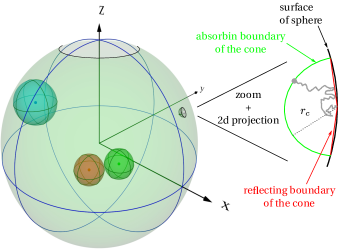
Figure 4: Illustration for the choices of protecting spheres/cones: The blue particle on the left is closer to the boundary of the simulation sphere than to any other particle, in consequence the radius of its protecting sphere is limited by the distance to the boundary. The green and the red particle in the middle are closer to each other than to the cell boundary. If they can react, their radius is limited by their distance. The gray particle has reached the boundary. Hence it is propagated in a cone, which is illustrated in the 2d projection.

Based on the solution of the diffusive initial value problem in $G$ (appendix Eq. (41)) it is possible to generate stochastically a first-passage time $t_{b}=t_{0}+\tau_{b}$ to the boundary of $G$, where $\tau_{b}$ is sampled according to the corresponding first-passage time probability $\rho_{b}$ (appendix Eq. (A.2)). If the particle does not switch to ballistic movement before time $t_{b}$, a random position update to the boundary of the sphere $G$ is done and a new protective domain must be assigned to the particle afterwards. Otherwise a new particle position within the sphere $G$ is sampled by using the radial probability density $\rho_{n}$ (appendix Eq. (A.2))

Due to the fact, that the boundaries of the sphere $V$ and the protecting sphere $G$ have always only one point in common, it does not work to use only spheres for the protecting domains. With probability one, the particle will touch the boundary of the simulation sphere, i.e. we would end up with an infinite sequence of protecting spheres, whose radii converge to zero. The best possibility to overcome this problem would be the usage of protection domains, whose boundaries coincide locally with the boundary of the simulation sphere in an area and not just in one point. Due to the missing knowledge of corresponding Green’s functions and/or the ability to sample efficiently within these domains, this is not possible. In consequence, for $d_{\partial V}\leq\epsilon_{R}$, we locally approximate the boundary of the simulation sphere by a suitable geometry, which is a spherical cone with a reflecting conical and an absorbing spherical boundary (appendix Eq. (44)). An example for such a situation is the gray particle in Fig. 4. If the distance to the boundary is larger than $\epsilon_{R}$ after being propagated within the cone, we again go on with a protecting sphere, otherwise, we use again a cone. The accuracy of this method is tunable via the two geometry boundary approximation parameters $\epsilon_{R}$ and the maximum radius $R_{pro}=r_{c}$ of the protecting cone. It is important to mention, that $r_{c}$ is just an upper limit for the cone’s radius. If the center position $\mathbf{x}_{c}\in\,\partial V\setminus A$ of the cone is closer than $r_{c}$ to the target area $A$, $R_{pro}$ is chosen to be the minimal distance of $\mathbf{x}_{c}$ to $A$.

In order to demonstrate the high accuracy, we compared our Monte Carlo method with the solution of a commercial FEM solver for a purely diffusive narrow escape problem. Starting at $r_{0}=0$, the searcher has the find the escape area with polar angle $\vartheta_{abso}=\pi/12$ (bright area at the top in Fig. 4). The FEM simulation was done on a very fine triangulation ($\approx$ 200000 elements) using the rotation symmetry of the problem and yields the expectation value $EW_{FEM}=4.1972R^{2}/D$ for the needed search time. The Monte Carlo simulation with $10^{7}$ samples was done for the geometry approximating parameters $\epsilon_{R}=10^{-4}\,R$, $r_{c}=0.04\,R$ and yields the almost perfectly matching value $EW_{MC}=4.1984R^{2}/D$. A much stronger criterion than the comparison of expectation values is the equality of the survival probability $S(t)$ (probability of not having reached the escape area until $t$) for all $t>0$. The again almost perfectly matching result is shown in Fig. 5.

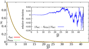
Figure 5: Comparison of the Monte Carlo method and the solution of a FEM solver on the basis of the survival probability $S(t)$ for a purely diffusive narrow escape process with $\vartheta_{abso}=\pi/12$ and $r_{0}=0$. The inset shows the very small relative deviation of these distributions.

All numerical results of this article are expected to be in the same numerical exactness (expect the sampling deviation in the case of a smaller number of samples), as the values of $\epsilon_{R}$ and $r_{c}$ where always chosen to be on the save side according to the smallest occurring length scale. However, the accuracy was successfully checked wherever this was possible (either by analytic values or FEM values).

For a diffusive particle at position $\mathbf{r}$, the total rate for a switch to a ballistic movement in an arbitrary direction $\Omega$ is given by $k(\mathbf{r},t)$ (see Eq. (4)). If this rate is spatially inhomogeneous, the methods of Zon2005a ; Zon2005b ; oppelstrup2006 ; oppelstrup2009 ; donev2010 will fail, as there is in general no analytic solution (Green’s function) to the diffusion-annihilation equation available. The algorithm, presented in schwarz2013 , overcomes this problem by using a spatially maximal rate

$$k_{m}(t)={\rm max}_{\mathbf{r}\in V}\{k(\mathbf{r},t)\}\;$$ (23)

in order to sample a candidate time $t_{\text{cand}}$ for a switch from diffusive to ballistic motion according to the probability density

$$\rho_{m}(t|t_{0})=-\frac{d}{dt}\left[e^{-\int_{t_{0}}^{t}k_{m}(t^{\prime})dt^{\prime}}\right]\;.$$ (24)

A new position $\mathbf{r}$ is assigned to the particle with the help of $\rho_{n}(\cdot|t_{\text{cand}}-t_{0})$ (appendix Eq. (A.2)). With probability $1-k(\mathbf{r},t_{\text{cand}})/k_{m}(t_{\text{cand}})$ the particle moves on diffusively. With probability $k(\mathbf{r},t_{\text{cand}})/k_{m}(t_{\text{cand}})$ it switches to ballistic motion with velocity $\mathbf{v}$, sampled according to the probability density $\rho_{\mathbf{v}}(\Omega|\mathbf{r},t)$ (see Eq. (5)).
For a back switch to diffusive motion only a corresponding time must be sampled, as there is a one-to-one relation between time and space in the case of ballistic motion.
For a better understanding, the pseudo-code details are shown in Algorithm 1, exemplarily for the BD boundary condition.

Algorithm 1 one particle

1:Input: $\mathbf{r}_{0}\in\mathbbm{R}^{3}$

2:Output: $\mathbf{r},t$

3:$t\leftarrow 0$;

4:$t_{\text{cand}}\leftarrow 0$;

5:$diffusive\leftarrow true$;

6:repeat

7:     if ( $diffusive$ ) then

8:         if ($t_{\text{cand}}\leq t$) then

9:              $t_{\text{cand}}\leftarrow$ random number according to $\rho_{m}(\cdot|t)$;

10:         end if

11:         Choose the protecting sphere/cone $P$ with            maximal radius $R_{pro}$ as a function of $\mathbf{r}$;

12:         $t_{b}\leftarrow$ $t$ + random number according to $\rho_{b}(\cdot)$            for $R_{pro}$;

13:         if ($t_{b}<t_{\text{cand}}$) then

14:              $\mathbf{r}\leftarrow$ rand. position at absorbing part of $\partial P$;

15:              $t\leftarrow t_{b}$;

16:         else

17:              $\mathbf{r}\leftarrow$ rand. position update within $P$ according                   to $\rho_{n}(\cdot|t_{\text{cand}}-t)$;

18:              $t\leftarrow t_{\text{cand}}$;

19:              if $\left(k(\mathbf{r},t)/k_{m}(t)\geq ran[0;1]\right)$ then

20:                  $diffusive\leftarrow false$;

21:                  $\mathbf{v}\leftarrow$ random velocity according to $\rho_{\mathbf{v}}(\cdot|\mathbf{r},t)$;

22:              end if

23:         end if

24:     else

25:         $t_{b}\leftarrow$ time when ballistic particle hits boundary;                   $(\;||\mathbf{r}+(t_{b}-t)\cdot\mathbf{v}||=R\,,\,\,t_{b}>t\;)$

26:         $t_{\text{cand}}\leftarrow$ random exponentially distributed number                   with rate $\gamma^{\prime}$;

27:         if ($t_{b}<t_{\text{cand}}$) then

28:              $\mathbf{r}\leftarrow\mathbf{r}+(t_{b}-t)\cdot\mathbf{v}$;

29:              $t\leftarrow t_{b}$;

30:         else

31:              $\mathbf{r}\leftarrow\mathbf{r}+(t_{\text{cand}}-t)\cdot\mathbf{v}$;

32:              $t\leftarrow t_{\text{cand}}$;

33:         end if

34:         $diffusive\leftarrow true$;

35:     end if

36:until  (distance to absorbing part of sphere $<$ threshold)

37:return $(\mathbf{r},t)$

III.2 interacting particle in a sphere of Radius $R$

If there are at least two particles in the simulation sphere, which are able to react, the choice of the protection boxes does not only depend on the position of the particle, but also on the distance between these reacting particles. In general, protecting spheres/cones of reacting particles are not allowed to be closer to each other than the interaction distance $d_{i}$. An example for such a situation is the red and green particle in the middle of Fig. 4. A similar problem as the boundary approximating problem in the subsection before has to be solved here. If we choose the protecting spheres/cones of interacting particles always in a way, that the boundaries of these protection boxes have their minimal distance in only one point, we will for sure end up in an infinite sequence of protection spheres/cones, whose radii tend to zero. In general there are two ways to overcome this problem. The first one is discussed in Zon2005b and the problem is solved via a coordinate transformation for the two particle positions to the difference vector and the mass point vector. As the problem factorizes in these coordinates, one ends up with two independent problems. Although a position update takes more time in these situations due to the fact, that radial symmetry is lost within the protection boxes in these coordinates, this is a very powerful tool for particles, which are far away (compared to their distance) from the boundary of the simulation sphere. But for particles, whose distance to the boundary is only a little bit larger than their distance to each other, this method does not work well. Hence, we decided to use a second tunable approximation by defining a parameter $\epsilon_{dist}$: If the distance between two reactive particles is less than $d_{i}+\epsilon_{dist}$ these particles react. If we choose $\epsilon_{dist}=10^{-4}\cdot d_{i}$, we are numerically for sure on the safe side, as all results look totally the same as in the case $\epsilon_{dist}=5\cdot 10^{-4}\cdot d_{i}$. A comparison to the solution of a FEM solver is not possible anymore, even for purely diffusive particles, due to the high spatial dimension ($2\cdot 3=6$) of the problem. A pseudo-code description would be quite large and the general idea is the same as in Algorithm 1. The interested reader is again referred to Zon2005a ; Zon2005b ; oppelstrup2006 ; oppelstrup2009 ; donev2010 ; schwarz2013 .

IV Narrow escape problem

The narrow escape problem for a purely diffusive particle in a sphere (and other simple domains) has already been studied in several publications. A nice overview, containing analytic asymptotic expressions, is given in Cheviakov2012 and Schuss2012 . Within this section, we consider the problem of a particle, which moves according to an intermittent search strategy, meaning, the master-equation system of its movement is given by the Eqs. (10) and (11) until it reaches the absorbing part of the boundary of the simulation sphere for the first time. This escape area is given by a spherical cab with polar angle $\vartheta_{\text{abso}}$, like it is shown at the north pole of Fig. 4. The position of this cap is of course not known by the particle.
The MFPT $\tilde{T}$ to the absorbing cap is a function of $\vartheta_{\text{abso}},\tilde{D},\tilde{\gamma},\tilde{\gamma}^{\prime}$ and the velocity direction distribution $\rho_{\mathbf{v}}(\Omega|\tilde{r})$. Furthermore, it depends on the initial position of the diffusively starting particle. But in the case of small target areas, the relative influence of the initial position totally vanishes. Depending on the diffusivity $\tilde{D}$ and $\vartheta_{\text{abso}}$, we study the optimal solution to the escape problem, i.e. we always look for the transition rates $(\tilde{\gamma},\tilde{\gamma}^{\prime})$ which minimize $\mathbb{T}$ (and simultaneously $\tilde{T}$).

purely diffusive search

The reference time $\tilde{T}_{\text{diff}}$ for a purely diffusive searcher ($\tilde{\gamma}^{\prime}\rightarrow\infty$ and/or $\tilde{\gamma}=0$) is inversely proportional to the diffusivity $\tilde{D}$. Among others, Cheviakov2012 has derived a very exact analytic approximation $\tilde{T}_{\text{diff}}^{\text{appro}}(\vartheta_{abso})$ of the problem for small $\vartheta_{abso}$ for arbitrary starting positions $\tilde{\mathbf{r}}_{0}$. For $\tilde{\mathbf{r}}_{0}=0$,

$$\tilde{T}_{\text{diff}}^{\text{appro}}(\vartheta_{abso})=\frac{1}{\tilde{D}}\left({\frac{\pi}{3\vartheta_{abso}}-\frac{1}{3}\text{ln}(2\vartheta_{abso})}\right)$$ (25)

holds. $\tilde{T}_{\text{diff}}$ has been calculated via $2\cdot 10^{6}$ $(\vartheta_{abso}\leq 0.15)$ - $10^{7}$ $(\vartheta_{abso}>0.15)$ Monte Carlo samples for each $\vartheta_{abso}$ and compared to the analytic approximation in Eq. (25). The result is shown in Fig. 6.

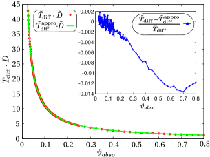
Figure 6: $\tilde{T}_{\text{diff}}\cdot\tilde{D}$ and $\tilde{T}_{\text{diff}}^{\text{appro}}\cdot\tilde{D}$ as a function of $\vartheta_{abso}$ for $\tilde{\mathbf{r}}_{0}=0$: Each red dot is the average of $2\cdot 10^{6}\;-\;10^{7}$ Monte Carlo samples. It coincides very well with the analytic approximation of Cheviakov2012 (green line), given in Eq. (25). The inset shows the relative difference between the curves.

For small values of $\vartheta_{abso}$ the relative deviation between the simulated value of $\tilde{T}_{\text{diff}}(\vartheta_{abso})$ and $\tilde{T}_{\text{diff}}^{\text{appro}}(\vartheta_{abso})$ is extremely small and only based on stochastic fluctuations (inset of Fig. 6 ). For larger values of $\vartheta_{abso}$ it slightly increases, which is not based on a drop of exactness in our numerical routines, but on the fact that the approximation $\tilde{T}_{\text{diff}}^{\text{appro}}$ becomes worse for larger opening angles. If the initial position $\tilde{\mathbf{r}}_{0}$ of the particle is equally distributed within the sphere, $\tilde{T}_{\text{diff}}$ and $\tilde{T}_{\text{diff}}^{\text{appro}}$ exactly decrease by $1/(10\tilde{D})$ for all $\vartheta_{abso}$, which has also been checked numerically.

random velocity model

Before studying intermittent strategies, it is insightful to have a look at the opposite choice of transitions rates $\tilde{\gamma}$ and $\tilde{\gamma}^{\prime}$, which is a random velocity model, given by the limit $\tilde{\gamma}\rightarrow\infty$ and $\tilde{\gamma}^{\prime}=0$.
For the BB boundary condition the corresponding MFPT $\tilde{T}_{\text{v}}$ tends trivially to infinity for all $\vartheta_{abso}\in[0;\pi]$, as the ballistically moving particle is reflected at the boundary without target area detection and never switches to diffusive mode (see Fig. 1b).

For the BD boundary condition, this is not the case. The resulting random velocity model is given by a ballistically moving particle, which detects the escape area at the boundary when reaching it and randomly chooses a new direction for the ballistic motion when reaching a part of the sphere’s boundary which does not belong to the target area. In consequence, the corresponding MFPT $\tilde{T}_{\text{v}}$ depends on the velocity direction distribution $\rho_{\mathbf{v}}(\Omega|\tilde{\mathbf{r}})$, the opening angle $\vartheta_{abso}$ and slightly on the initial position $\tilde{\mathbf{r}}_{0}$. For $\tilde{\mathbf{r}}_{0}=0$ and the case of a homogeneous velocity direction density (Eq. 14) we derived an approximating expression $\tilde{T}_{\text{v}}^{\text{appro}}(\vartheta_{abso})$ for $\vartheta_{abso}\in[0;\pi/2]$:

$$\tilde{T}_{\text{v}}^{\text{appro}}(\vartheta_{abso})=1+\frac{1+\cos(\vartheta_{abso})}{2}\cdot\Psi(\vartheta_{abso})$$ (26)

$$\text{with }\;\;\Psi(x)=\frac{1+\cos(x)}{1-\cos(x)}\times\hskip 42.67912pt$$

$$\frac{1}{\frac{\cos(x)-1}{\sin(x)}+x\sin(x)+4\cos\left({\frac{x}{2}}\right)-3-4\cos(x)\ln\left({\frac{\cos(\frac{x}{4})}{\cos(\frac{x}{2})}}\right)}\;.$$

Fig. 7 shows $\tilde{T}_{\text{v}}$ ($10^{8}$ samples) and $\tilde{T}_{\text{v}}^{\text{appro}}$ in a logscale plot. The relative deviation of $\tilde{T}_{\text{v}}$ and $\tilde{T}_{\text{v}}^{\text{appro}}$ vanishes for $\vartheta_{abso}\rightarrow 0$, which is shown in the inset.

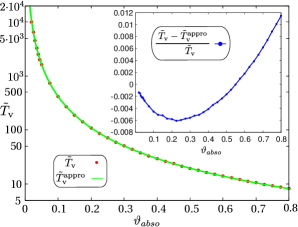
Figure 7: $\tilde{T}_{\text{v}}$ and $\tilde{T}_{\text{v}}^{\text{appro}}$ as a function of $\vartheta_{abso}$ for $\tilde{\mathbf{r}}_{0}=0$: Each red dot is the average of $10^{8}$ Monte Carlo samples. It coincides very well with the analytic approximation $\tilde{T}_{\text{v}}^{\text{appro}}$ (green line), given in Eq. (26). The inset shows the relative difference between the curves.

If the initial position $\tilde{\mathbf{r}}_{0}$ of the particle is equally distributed within the sphere, $\tilde{T}_{\text{v}}$ and $\tilde{T}_{\text{v}}^{\text{appro}}$ exactly decrease by $1/4$ for all $\vartheta_{abso}$.

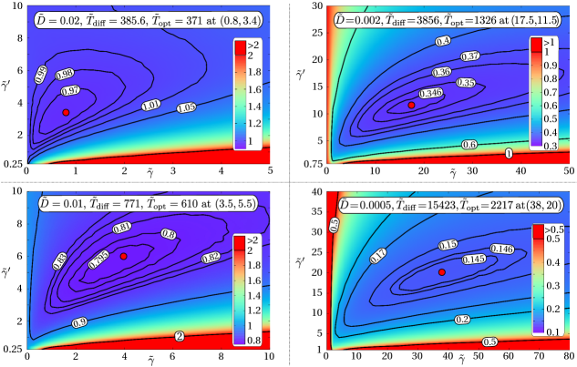
Figure 8: narrow escape, BB, $\rho_{\text{hom}}^{\alpha}$; The normalized MFPT $\mathbb{T}$ (Eq. 1) is color-coded as a function of the rates $\tilde{\gamma}$ and $\tilde{\gamma}^{\prime}$ for different values of $\tilde{D}$ and $\vartheta_{\text{abso}}=\text{arcsin}(1/7)$ (interpolation from a grid of $41\times 41$ data points each). $2-5\cdot 10^{6}$ samples have been done for each pair ($\tilde{\gamma}$ , $\tilde{\gamma}^{\prime}$), which leads to relative stochastic fluctuations of $\mathbb{T}$, which are smaller than 0.2%. The position of the minimum $(\tilde{\gamma}_{\text{opt}},\tilde{\gamma}^{\prime}_{\text{opt}})$ is always shown with a red dot.

A comparison of $\tilde{T}_{\text{diff}}^{\text{(appro)}}$ and $\tilde{T}_{\text{v}}^{\text{(appro)}}$ points out an important difference in the behavior of divergence of $\tilde{T}_{\text{diff}}$ and $\tilde{T}_{\text{v}}$ for small escape areas:

$$\tilde{T}_{\text{diff}}(\vartheta_{abso}) \propto \frac{1}{\tilde{D}\cdot\vartheta_{abso}}$$

$$\tilde{T}_{\text{v}}(\vartheta_{abso}) \propto \left\{\begin{array}[]{ccc}\infty&,&\text{BB boundary cond.}\\ \frac{1}{(\vartheta_{abso})^{2}}&,&\text{BD boundary cond.}\end{array}\right.\;.$$ (29)

After having studied the two possible extreme cases in search behavior, which is necessary for understanding the later discussed $\vartheta_{\text{abso}}$ dependence, we now face intermittent strategies and analyze their efficiency.

In subsection IV.1 the condition BB is studied, i.e. a ballistically moving particle, which hits the boundary of the simulation sphere, stays in its ballistic mode with the reflected velocity direction. The arrival at the escape area of the sphere will only be detected if the particle is in the diffusive mode, otherwise it is reflected. We compare the problem of the homogeneously distributed direction density $\rho_{\text{hom}}^{\alpha}$ to the inhomogeneous scenario of $\rho_{x}^{\alpha}$.
In subsection IV.2 the condition BD is studied, i.e. a ballistically moving particle, which hits the boundary of the simulation sphere, switches immediately to the diffusive mode, i.e. if this switch happens at the escape area, the particle immediately recognizes the exit. Here, the homogeneous case is compared to the inhomogeneous scenarios of $\rho_{x}^{\alpha}$ and $\rho_{p,\tilde{\Delta}}^{\alpha}$.

IV.1 BB

For the BB condition, the searcher will start in the center of the sphere and the escape area is given by a spherical cab with angle $\vartheta_{\text{abso}}=\text{arcsin}(1/7)\approx 0.1433$ within this subsection, i.e. the radius of the absorbing spherical cab is seven times smaller then the radius of the sphere. In consequence, the area the particle searches, is about $0.51\%$ of the total spherical surface, i.e. we are in the limit of a small escape area. In this setup, the reference time (taken from the MC data of Fig. 6) is given by

$$\tilde{T}_{\text{diff}}=\frac{7.71}{\tilde{D}}\;.$$ (30)

IV.1.1 homogeneous distribution $\rho^{\alpha}_{\text{hom}}$

For different values of $\tilde{D}$, we look for the best strategy to search for the absorbing area as a function of the switching parameters $\tilde{\gamma}$ and $\tilde{\gamma}^{\prime}$. $\mathbb{T}$ as a function of $\tilde{\gamma}$ and $\tilde{\gamma}^{\prime}$ is shown in Fig. 8 for four different examples of $\tilde{D}$. For $\tilde{D}=\frac{D}{vR}$ larger than about 0.025 there is no benefit in a mixed strategy. Here, a purely diffusive particle is on average the better searcher as diffusive motion is faster on these scales. As $\tilde{D}$ decreases, phases of ballistic displacement become more and more efficient, as the diffusive displacement per time unit shrinks. Hence, a global minimum $\mathbb{T}_{\text{opt}}(\tilde{D})=\tilde{T}_{\text{opt}}(\tilde{D})/\tilde{T}_{\text{diff}}(\tilde{D})<1$ occurs in the ($\tilde{\gamma},\tilde{\gamma}^{\prime}$) space, i.e. there is a benefit in an intermittent search strategy. As expected, this benefit further increases with decreasing $\tilde{D}$, i.e. $\mathbb{T}_{\text{opt}}(\tilde{D})$ increases monotonically and

$$\lim_{\tilde{D}\rightarrow 0^{+}}\mathbb{T}_{\text{opt}}(\tilde{D})=0$$ (31)

holds, although $\lim_{\tilde{D}\rightarrow 0^{+}}\tilde{T}_{\text{opt}}(\tilde{D})=\infty$. Surprisingly, the efficiency of the strategy changes only very little in a quite large (relative to the absolute values) surrounding of the optimal solution $(\tilde{\gamma}_{\text{opt}},\tilde{\gamma}^{\prime}_{\text{opt}}$) for all diffusivities $\tilde{D}$. This can be seen by having a closer look to the values of the isolines in Fig. 8. In consequence, due to stochastic fluctuations, the relative error in the optimal values of $\tilde{\gamma}_{\text{opt}}$ and $\tilde{\gamma}^{\prime}_{\text{opt}}$ is much larger than the relative error in the value of $\tilde{T}_{\text{opt}}$ and $\mathbb{T}_{\text{opt}}$. Fig. 9 shows $\tilde{\gamma}_{\text{opt}}$, $\tilde{\gamma}^{\prime}_{\text{opt}}$ and (in the inset) $\mathbb{T}_{\text{opt}}$ as a function of the diffusivity $\tilde{D}$.

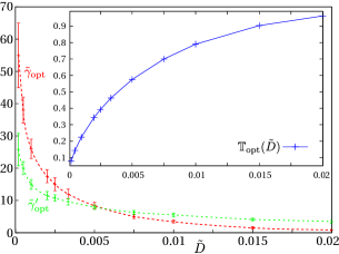
Figure 9: narrow escape, BB, $\rho_{\text{hom}}^{\alpha}$; The optimal transition rates $\tilde{\gamma}_{\text{opt}}$, $\tilde{\gamma}^{\prime}_{\text{opt}}$ and the resulting normalized MFPT $\mathbb{T}_{\text{opt}}$ (inset) as a function of $\tilde{D}$. For the diffusion coefficients shown in Fig. 8, the data coincides with the coordinates of the red dots and its value of $\mathbb{T}$.

The corresponding values of $\tilde{T}_{\text{diff}}$ and $\tilde{T}_{\text{opt}}$ are also listed in Table 1 and plotted in Fig. 11 for a comparison to the later treated inhomogeneous search scenarios. $\tilde{\gamma}_{\text{opt}}$ and $\tilde{\gamma}^{\prime}_{\text{opt}}$ decrease monotonically in $\tilde{D}$. As this happens faster for $\tilde{\gamma}$ than for $\tilde{\gamma}^{\prime}$, the fraction of time spend in the diffusive mode $\tilde{\gamma}^{\prime}/(\tilde{\gamma}+\tilde{\gamma}^{\prime})$ increases with $\tilde{D}$.

Due to the enormous numerical effort, it is not possible to vary $\vartheta_{\text{abso}}$ systematically here. Nevertheless, we exemplarily investigated also some values of $\tilde{D}$ for smaller and larger values of $\vartheta_{\text{abso}}$. Similar to the results in the following chapters, we found, that a decrease in target size results in an increase in both transition rates.

IV.1.2 inhomogeneous distribution $\rho_{x}^{\alpha}$

Within this subsubsection, we study the influence of $\rho_{x}^{\alpha}$ on the search strategy and the transition rates. Fig. 10 shows the dependence of $\mathbb{T}$ on $x$ for representatively selected values of $\tilde{D}$ and the corresponding optimal parameters $\tilde{\gamma}_{\text{opt}}(\tilde{D}),\;\tilde{\gamma}^{\prime}_{\text{opt}}(\tilde{D})$ of the homogeneous scenario, shown in Fig. 9.

The global minimum for each $\tilde{D}$ will be denoted $\tilde{T}_{\text{min}}(\tilde{D})$ in the following.

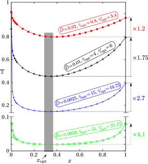
Figure 10: narrow escape, BB, $\rho_{x}^{\alpha}$; $\mathbb{T}$ as a function of the spreading parameter $x$ for the transition rates $(\tilde{\gamma}_{\text{opt}},\tilde{\gamma}^{\prime}_{\text{opt}})$ of the optimal solution of Fig. 9. The minimum position $x_{\text{opt}}\approx 0.35$ (gray bar) of all curves is almost identical. The colored numbers on the right show the ratio $\mathbb{T}_{\text{min}}/\mathbb{T}_{\text{opt}}$.

At $x=1$ the values of $\mathbb{T}$ coincide with the corresponding $\mathbb{T}_{\text{opt}}$ of Fig. 9. In none of the cases, the value at $x=1$ is the minimum. It follows, that an anisotropic velocity direction distribution increases the efficiency of the search strategy significantly. For small values of $\tilde{D}$, $\tilde{T}_{\text{min}}$ is much smaller than $\tilde{T}_{\text{opt}}$, which can also be seen by comparing the blue and the green curves of Fig. 11 and the corresponding values in Table 1. As $\tilde{D}$ increases the benefit of an inhomogeneous strategy becomes less pronounced. It is remarkable, that the degree of inhomogeneity $x_{\text{opt}}\approx 0.35$ is constant for all $\tilde{D}$.

Nevertheless it is even possible to decrease $\mathbb{T}$ further: In Fig. 10 the transition rates were chosen as the optimal solution for the homogeneous case. There is no reason, that this is also the optimal choice in the inhomogeneous case. In consequence, we varied $\tilde{\gamma},\;\tilde{\gamma}^{\prime}$ and $x$ simultaneously for finding the optimal parameters $\tilde{\Gamma}\text{\textsubscript{\tiny OPT}},\;\tilde{\Gamma}^{\prime}\text{\textsubscript{\tiny OPT}}$ and $X\text{\textsubscript{\tiny OPT}}$ for the MFPT $\tilde{T}\text{\textsubscript{\tiny OPT}}$ (be aware of the different meaning of the index ”opt“ and ”OPT“). The results are shown in Table 1 and $\tilde{T}\text{\textsubscript{\tiny OPT}}$ is plotted in Fig. 11.

$\tilde{D}$	$\tilde{T}_{\text{diff}}$	$\tilde{T}_{\text{opt}}$	$\tilde{T}_{\text{min}}$	$\tilde{T}\text{\textsubscript{\tiny OPT}}$	$\tilde{\gamma}_{\text{opt}}$	$\tilde{\gamma}^{\prime}_{\text{opt}}$	$\tilde{\Gamma}\text{\textsubscript{\tiny OPT}}$	$\tilde{\Gamma}^{\prime}\text{\textsubscript{\tiny OPT}}$	$x_{\text{opt}}$	$X\text{\textsubscript{\tiny OPT}}$
0.02	386	371	307	238	0.8	3.4	11.5	8	0.35	0.325
0.015	514	465	337	264	1.5	4.1	18	8.5	0.35	0.325
0.01	771	610	349	297	4	6	25	9.5	0.35	0.325
0.0075	1028	720	377	321	5	6.3	30	10	0.35	0.325
0.005	1542	888	398	353	8.4	7.9	36	11	0.35	0.325
1/300	2314	1071	433	386	12	9.6	42	12	0.35	0.325
$0.0025$	3085	1211	448	410	15	10.75	48	13	0.35	0.325
0.002	3856	1326	466	429	17.5	11.5	50	13.5	0.35	0.325
0.001	7712	1727	530	492	26	15	60	15	0.35	0.3
$0.0005$	15420	2217	618	562	38	20	75	18	0.35	0.3
$0.0002$	38560	3026	740	670	55	25.75	95	21	0.35	0.3

Table 1: $\tilde{T}_{\text{diff}}$: purely diffusive MFPT; $\tilde{T}_{\text{opt}}$: optimized intermittent MFPT for $\rho_{\text{hom}}^{\alpha}$ with optimal rates $\tilde{\gamma}_{\text{opt}}$ and $\tilde{\gamma}^{\prime}_{\text{opt}}$; $\tilde{T}_{\text{min}}$: optimized intermittent MFPT for $\rho_{x}^{\alpha}$ with optimal inhomogeneity coefficient $x_{\text{opt}}$ and fixed rates $\tilde{\gamma}_{\text{opt}}$ and $\tilde{\gamma}^{\prime}_{\text{opt}}$; $\tilde{T}\text{\textsubscript{\tiny OPT}}$: optimized intermittent MFPT for $\rho_{x}^{\alpha}$ with optimal inhomogeneity coefficient $X\text{\textsubscript{\tiny OPT}}$ and corresponding optimal rates $\tilde{\Gamma}\text{\textsubscript{\tiny OPT}}$ and $\tilde{\Gamma}^{\prime}\text{\textsubscript{\tiny OPT}}$.

Table 1 delivers some remarkable results:

• The optimal value of $x$ seems to be almost constant in all cases. For the rates of the homogeneous optimization $(\tilde{\gamma}_{\text{opt}},\tilde{\gamma}^{\prime}_{\text{opt}})$ and for the rates of the inhomogeneous optimization $(\tilde{\Gamma}\text{\textsubscript{\tiny OPT}},\tilde{\Gamma}^{\prime}\text{\textsubscript{\tiny OPT}})$ the best solution is always given by $x\approx 0.325\pm 0.025$. Hence, the degree of inhomoegeneity for an optimal solution does not seem to depend much on the diffusion coefficient and the transition rates, which is quite surprising.

• Comparing the values of $(\tilde{\gamma}_{\text{opt}},\tilde{\gamma}^{\prime}_{\text{opt}})$ with $(\tilde{\Gamma}\text{\textsubscript{\tiny OPT}},\tilde{\Gamma}^{\prime}\text{\textsubscript{\tiny OPT}})$, one recognizes remarkable changes in the transition rates. For large values of $\tilde{D}$, the change is more than a factor of 10.

• Like in the homogeneous case, the efficiency of the inhomogeneous strategy changes only very little in a quite large surrounding of the optimal solution $(\tilde{\Gamma}\text{\textsubscript{\tiny OPT}},\tilde{\Gamma}^{\prime}\text{\textsubscript{\tiny OPT}})$.

For concluding this subsection, Fig. 11 shows the optimal MFPTs for the different discussed scenarios.

Figure 11: narrow escape, BB; MFPT for purely diffusive search (Eq. 30, red line); optimal search with homogeneously distributed velocity direction (green); optimal search with inhomogeneously distributed velocity direction for the fixed rates $\tilde{\gamma}_{\text{opt}}$, $\tilde{\gamma}^{\prime}_{\text{opt}}$ for the homogeneous scenario (blue) ; optimal search with inhomogeneously distributed velocity direction for rates $\tilde{\Gamma}_{\text{\textsubscript{\tiny OPT}}}$, $\tilde{\Gamma}^{\prime}_{\text{\textsubscript{\tiny OPT}}}$ (black).

Compared to a purely diffusive searcher (red), an intermittent search strategy with a homogeneous velocity direction distribution (green) optimizes the search process especially for small $\tilde{D}$ significantly, which has already been shown in the inset of Fig. 9. In the next step, we introduced an inhomogeneity in the velocity direction distribution (blue), but kept the optimal rates of the homogeneous case. Again, the largest benefit can be seen for small $\tilde{D}$ (see Fig. 10). In the last step, we varied the transition rates and the degree of inhomogeneity simultaneously (black). Although the optimal rates changed dramatically, the additional benefit is much smaller than in the optimization steps before. But this time it increases with $\tilde{D}$.

IV.2 BD

For all investigated direction distributions ($\rho_{\text{hom}}^{\alpha}$ and both inhomogeneous scenarios $\rho_{x}^{\alpha}$, $\rho_{p,\tilde{\Delta}}^{\alpha}$ ) in this subsection the optimal search strategy is either a purely diffusive one (for $\tilde{D}$ large) or the simulations yield $\tilde{\gamma}^{\prime}_{\text{opt}}=0$. Exemplarily, this is shown in Fig. 12. For $\vartheta_{abso}=\text{arcsin}(1/7)$ and different values of $\tilde{D}$ the figure shows $\mathbb{T}$ as a function of the transition rates for the case of $\rho_{\text{hom}}^{\alpha}$ and the initial position in the origin.

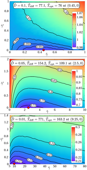
Figure 12: narrow escape, BD, $\rho_{\text{hom}}^{\alpha}$; The normalized MFPT $\mathbb{T}$ (Eq. 1) is color-coded as a function of the parameters $\tilde{\gamma}$ and $\tilde{\gamma}^{\prime}$ for different values of $\tilde{D}$ and $\vartheta_{\text{abso}}=\text{arcsin}(1/7)$ (interpolation from a grid of $41\times 41$ data points each). Between $2\cdot 10^{6}$ and $5\cdot 10^{6}$ samples have been done for each pair ($\tilde{\gamma}$ , $\tilde{\gamma}^{\prime}$), which leads to relative stochastic fluctuations of $\mathbb{T}$ which are smaller than 0.2% for. The position of the minimum $(\tilde{\gamma}_{\text{opt}},\tilde{\gamma}^{\prime}_{\text{opt}})$ is always shown with a red dot.

A comparison to Fig. 8 shows the different behaviour of the optimal solution for the two boundary conditions. We verified $\tilde{\gamma}^{\prime}_{\text{opt}}=0$ also for smaller values of $\vartheta_{abso}$ and larger ones ($0.025<\vartheta_{abso}<\pi$). Consequently, the numerical effort of finding the best strategy is dramatically reduced, as there is one parameter less to vary. Due to this reduced effort, the variation of the absorbing angle $\vartheta_{\text{abso}}$ will also be studied in the case of a $\rho_{\text{hom}}^{\alpha}$.
Apart from this additional study, the beginning of the subsection is organized identically to the one before: We start with the case of $\rho_{\text{hom}}^{\alpha}$ , followed by the inhomogeneous scenario $\rho_{x}^{\alpha}$ for $\vartheta_{abso}=\text{arcsin}(1/7)$. In both cases the initial position is the origin. Afterwards we study the case $\rho_{p,\tilde{\Delta}}^{\alpha}$ for a homogeneously distributed initial position $\tilde{\mathbf{r}}_{0}$ and $\vartheta_{abso}=\text{arcsin}(1/7)$.

IV.2.1 homogeneous distribution $\rho_{\text{hom}}^{\alpha}$

At first, we study whether an intermittent search strategy or a purely diffusive strategy is better for a given pair of parameters ($\tilde{D},\,\vartheta_{abso}$). For the reason of completeness we faced this question for all values of $\vartheta_{abso}\in]0;\pi]$ and not only for a ”narrow” escape area. The result for $\tilde{\mathbf{r}}_{0}=0$ is shown in Fig. 13.

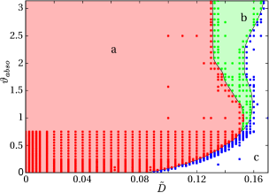
Figure 13: narrow escape, BD, $\rho_{\text{hom}}^{\alpha}$; Diagram for the choice of the best search strategy as a function of $\tilde{D}$ and $\vartheta_{abso}$ : In the red (a) and the green (b) domain, an intermittent search strategy is preferable, whereas in the white domain (c) pure diffusion is the best strategy. For the construction of the diagram, the behaviour at the position of the dots was investigated.

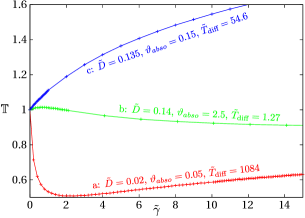
Figure 14: narrow escape, BD, $\rho_{\text{hom}}^{\alpha}$; Examples of the function $\mathbb{T}(\tilde{\gamma},\tilde{\gamma}^{\prime}_{\text{opt}}=0$) for the three different colored areas in Fig. 13.

In the red (a) domain an intermittent search strategy is preferable. $\mathbb{T}(\tilde{\gamma})$ starts monotonically decreasing at $\tilde{\gamma}=0$. It follows the global optimum at $\tilde{\gamma}_{\text{opt}}>0$. An example for this behavior for $\tilde{D}=0.02$, $\vartheta_{abso}=0.05$ is given in Fig. 14.
In the green domain (b), intermittent search is also preferable. Although $\mathbb{T}(\tilde{\gamma})$ starts monotonically increasing, it decreases to $\mathbb{T}<1$ for some values of $\tilde{\gamma}$. Again, an example for this behavior for $\tilde{D}=0.14$, $\vartheta_{abso}=2.5$ is given in Fig. 14.
Finally, in the white domain (c) $\tilde{\gamma}_{\text{opt}}=0$ holds, hence a diffusive search is the best strategy. An example for this behavior for $\tilde{D}=0.135$, $\vartheta_{abso}=0.15$ is also given in Fig. 14.

Fig. 13 only answers the question about the best strategy in principle, it is neither quantifying the transition rate $\tilde{\gamma}_{\text{opt}}(\tilde{D},\tilde{\vartheta}_{abso})$ nor the MFPTs $\tilde{T}_{\text{opt}}(\tilde{D},\tilde{\vartheta}_{abso})$ and $\mathbb{T}_{\text{opt}}(\tilde{D},\tilde{\vartheta}_{abso})$. A quantification has only been done in the case of small escape areas ($\vartheta_{abso}<0.75$) due to the following reasons:
If the escape area is large, the searcher will find it soon, hence there is no need for a special strategy. The largest impact of $\tilde{\gamma}$ on the efficiency of the strategy is given for small values of $\tilde{\vartheta}_{abso}$, i.e. for large $\tilde{\vartheta}_{abso}$ either a purely diffusive searcher or a random velocity model ($\tilde{\gamma}=\infty$) is always close to the optimal strategy. Additionally, for small values of $\vartheta_{abso}$ the optimal strategy is almost independent of the starting position of the searcher, i.e. the shown results for a searcher starting at the origin will remain true in the more general context of an arbitrary initial position. For the angle $\tilde{\vartheta}_{abso}=\text{arcsin}(1/7)$ this independence is shown explicitly later.

Fig. 15 quantifies the values of $\tilde{\gamma}$, $\tilde{T}_{\text{opt}}$ and $\mathbb{T}_{\text{opt}}$ for $0.025<\vartheta_{abso}<0.75$.

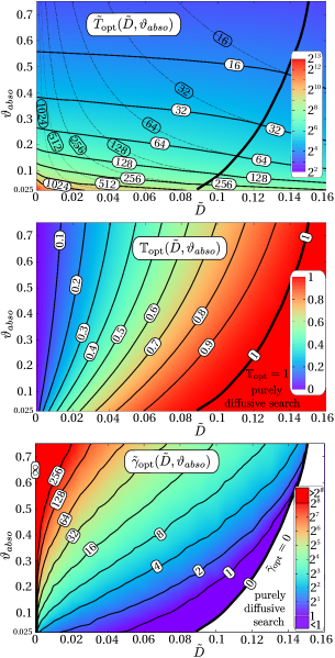
Figure 15: narrow escape, BD, $\rho_{\text{hom}}^{\alpha}$; $\tilde{T}_{\text{opt}}$, $\mathbb{T}_{\text{opt}}$ and the corresponding $\tilde{\gamma}_{\text{opt}}$ as a function of $\tilde{D}$ and $\vartheta_{abso}<0.75$ (interpolation from the non equidistant grid shown at the bottom of Fig. 13). The thick black line in each subfigure separates the area of intermittent search and purely diffusive search. It coincides with the boundary line between the area a and c in Fig. 13. top: $\tilde{T}_{\text{opt}}$ in a logscale color plot, the dashed lines with transparent label show isolines of the purely diffusive search scenario (Eq. (25)) for the reason of comparison. middle: $\mathbb{T}_{\text{opt}}$ is color-coded plotted bottom: $\tilde{\gamma}_{\text{opt}}$ in a logscale color plot.

The corresponding curves, from which the optimal values of $\tilde{\gamma}_{\text{opt}}$ and $\tilde{T}_{\text{opt}}$ were taken for each data point, qualitatively all look like the red curve in Fig. 14. Depending on $\tilde{D}$ and $\vartheta_{abso}$, $500.000$ up to $10^{10}$ samples have been performed for each parameter triple ($\tilde{\gamma}$, $\tilde{D}$, $\vartheta_{abso}$). As the depth of the minimum position is differently strong pronounced this is necessary to control the stochastic fluctuations in the value of $\tilde{\gamma}_{\text{opt}}$.
For $\tilde{D}=0$ the optimal strategy is trivially given by $\tilde{\gamma}_{\text{opt}}=\infty$ for all $\vartheta_{abso}$, i.e. the optimal strategy is the random velocity model with MFPT $\tilde{T}_{\text{v}}$, which is very well approximated by $\tilde{T}_{\text{v}}^{\text{(appro)}}$ in Eq. (26), shown in Fig. 7. For small diffusivities $\tilde{D}>0$ the transition rate $\tilde{\gamma}_{\text{opt}}$ is finite. Its value strongly depends on the size of the escape area, i.e. on the value of $\vartheta_{abso}$. The thick black line in Fig. 15 shows the ”break-even“ diffusivity $\tilde{D}_{\text{be}}(\vartheta_{abso})$, where the optimal strategy changes from intermittent search to purely diffusive search. $\tilde{D}_{\text{be}}$ increases monotonically in $\vartheta_{abso}$. It rises the interesting question about the limit of $\tilde{D}_{\text{be}}$ for $\vartheta_{abso}\rightarrow 0$ (be aware of $0.025<\vartheta_{abso}$ in Fig. 15). If $\lim_{\vartheta_{abso}\rightarrow 0}\tilde{D}_{\text{be}}=0$ held, for every $\tilde{D}$ there would be a threshold value $\vartheta_{thres}$ below which pure diffusion would be the best strategy. In the opposite case of a positive limit $\tilde{D}_{\text{be0}}$, i.e. $\lim_{\vartheta_{abso}\rightarrow 0}\tilde{D}_{\text{be}}=\tilde{D}_{\text{be0}}>0$, intermittent search would be more efficient for all $\tilde{D}<\tilde{D}_{\text{be0}}$, no matter how small $\vartheta_{abso}$ becomes. Due to the divergence of the MFPT for $\vartheta_{abso}\rightarrow 0$ it is not possible to face this limit numerically for the reason of running time. Nevertheless, there are clear arguments for a limit $\tilde{D}_{\text{be0}}>0$: The second derivatives of the isolines of $\mathbb{T}_{\text{opt}}$ in the second subfigure of Fig. 15 seems to vanish for small $\vartheta_{abso}$. Hence, they were expected to reach the x-axis in a straight line at positions larger than zero. Due to the enormous running time for very small angles we verified this hypothesis of affine extrapolation only partially at $\vartheta_{abso}=0.0125$ for some $\tilde{D}$.

For comparison to the boundary condition BB and the later investigated inhomogeneous search scenarios, the angle $\vartheta_{abso}=\text{arcsin}(1/7)$ is shown separately in Fig. 16 and the corresponding values of $\tilde{T}_{\text{opt}}$ are shown in Fig. 18 and Table 2.

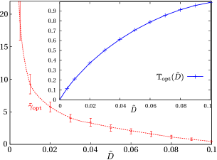
Figure 16: narrow escape, BD, $\rho_{\text{hom}}^{\alpha}$; $\tilde{\gamma}_{\text{opt}}$ and $\mathbb{T}_{\text{opt}}$ (inset) as a function of $\tilde{D}$ for $\vartheta_{\text{abso}}=\text{arcsin}(1/7)$: The corresponding curves $\mathbb{T}(\tilde{\gamma})$ from which the minima are taken qualitatively all belong to case (a) in the diagram. For $2\cdot 10^{6}$ samples for each investigated $\tilde{D}$ the position of the minimum $\tilde{\gamma}_{\text{opt}}$ and its value $\mathbb{T}_{\text{opt}}$ are shown.

Qualitatively, Fig. 16 does not differ from the result of Fig. 9 (except for $\tilde{\gamma}^{\prime}=0$), but quantitatively it differs a lot. The interval where an intermittent search strategy is preferable ($\tilde{D}<0.11$) is almost five times larger compared to the boundary condition BB. For the BD condition the benefit of an intermittent search strategy is always larger, for the following reason: A ballistically moving particle detects the target area immediately after switching to diffusive mode at the boundary. In the subsection before, the particle was simply reflected without recognizing the target area. In consequence, the status of the ballistic mode is enhanced here, which can also be seen by comparing the values of $\tilde{\gamma}_{\text{opt}}$ in the common interval of Fig. 9 and Fig. 16. In case of the BD condition of this subsection the searcher stays on average shorter in the diffusive mode before switching back to ballistic motion again compared to the BB scenario.

IV.2.2 inhomogeneous distribution $\rho_{x}^{\alpha}$

Fig. 17 shows $\mathbb{T}$ as a function of $x$ for the optimal parameters $\tilde{\gamma}_{\text{opt}}$ of Fig. 16 for different values of $\tilde{D}$. For each $\tilde{D}$ the minimal MFPT $\tilde{T}_{\text{min}}$ is plotted in Fig. 18 and listed in Table 2.

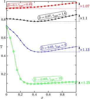
Figure 17: narrow escape, BD, $\rho_{x}^{\alpha}$; $\mathbb{T}$ as a function of the spreading parameter $x$ for the transition rate $\tilde{\gamma}_{\text{opt}}$ of the optimal solution of Fig. 16. The colored numbers on the right show the ratio $\mathbb{T}_{\text{min}}/\mathbb{T}_{\text{opt}}$.

For large values of $\tilde{D}$, $x_{\text{opt}}=0$ holds, meaning the optimal velocity direction is always radially to the outward. As $\tilde{D}$ decreases, the minimum $x_{\text{opt}}$ switches to the interior of the interval $[0,1]$. A comparison to Fig. 10 shows the following differences between the two boundary conditions: The position of $x_{\text{opt}}$ is not constant any more, here it depends strongly on $\tilde{D}$. The value of $\mathbb{T}_{min}$ at $x_{\text{opt}}$ differs less from the value of the homogeneous velocity direction distribution (x=1). Hence, the additional benefit of an inhomogeneous velocity direction is less than in the case of the previous subsection. This can also be seen by comparing the gap between the green and blue lines of Fig. 11 and Fig. 18.
Similar to the BB boundary condition before, we varied $\tilde{\gamma}$, $\tilde{\gamma}^{\prime}$ and $x$ simultaneously to find the optimal parameters $\tilde{\Gamma}_{\text{OPT}}$ and $X\text{\textsubscript{\tiny OPT}}$ for the MFPT $\tilde{T}\text{\textsubscript{\tiny OPT}}$. The optimal $\gamma^{\prime}$ again vanishes, i.e. $\tilde{\Gamma}^{\prime}_{\text{OPT}}=0$. The other results are shown in Table 2.

$\tilde{D}$	$\tilde{T}_{\text{diff}}$	$\tilde{T}_{\text{opt}}$	$\tilde{T}_{\text{min}}$	$\tilde{T}\text{\textsubscript{\tiny OPT}}$	$\tilde{\gamma}_{\text{opt}}$	$\tilde{\Gamma}\text{\textsubscript{\tiny OPT}}$	$x_{\text{opt}}$	$X\text{\textsubscript{\tiny OPT}}$
0.1	77.1	76	71	67.6	0.45	1.7	0	0
0.09	85.7	81.8	75.2	73.4	0.8	1.6	0	0
0.08	96.4	87.8	80.8	77.3	1.15	4	0.35	0.375
0.07	110	94.2	85.9	81.8	1.6	5.5	0.45	0.4
0.06	129	101	91.6	86.5	2	7.5	0.45	0.4
0.05	154	109	98	91.7	2.5	14	0.45	0.375
0.04	193	118	104	95.8	3.4	-	0.45	0.12
0.03	257	129	114	95.8	4	-	0.45	0.12
0.02	386	143	124	95.8	5.75	-	0.45	0.12
0.01	771	163	138	95.8	9.25	-	0.45	0.12
0.005	1542	178	142	95.8	19	-	0.4	0.12

Table 2: $\tilde{T}_{\text{diff}}$: purely diffusive MFPT; $\tilde{T}_{\text{opt}}$: optimized intermittent MFPT for $\rho_{\text{hom}}^{\alpha}$ with optimal rate $\tilde{\gamma}_{\text{opt}}$; $\tilde{T}_{\text{min}}$: optimized intermittent MFPT for $\rho_{x}^{\alpha}$ with optimal inhomogeneity coefficient $x_{\text{opt}}$ and fixed rate $\tilde{\gamma}_{\text{opt}}$; $\tilde{T}\text{\textsubscript{\tiny OPT}}$: optimized intermittent MFPT for $\rho_{x}^{\alpha}$ with optimal inhomogeneity coefficient $X\text{\textsubscript{\tiny OPT}}$ and corresponding optimal rate $\tilde{\Gamma}\text{\textsubscript{\tiny OPT}}$

A comparison of the table with Fig. 17 and the rates of Fig. 16 delivers some remarkable results:

• In contrast to the case of the BB condition, $x_{\text{opt}}$ varies a lot in the different optimization scenarios.

• Comparing the values of $\tilde{\gamma}_{\text{opt}}$ with $\tilde{\Gamma}\text{\textsubscript{\tiny OPT}}$, one recognizes remarkable changes in the transition rates. Especially for $\tilde{D}<0.05$, it is not possible to find $\tilde{\Gamma}\text{\textsubscript{\tiny OPT}}$ as it tends to infinity, i.e. the best strategy here is a random velocity search. A particle reaching the boundary, immediately switches to ballistic motion again. The velocity direction distribution is a renormalization of $\rho^{\alpha}_{0.12}$ to the interval $[\pi/2,\pi]$, as $\alpha<\pi/2$ is not possible for particles at the boundary.

For concluding this subsection, Fig. 18 shows the optimal MFPTs for the different discussed scenarios.

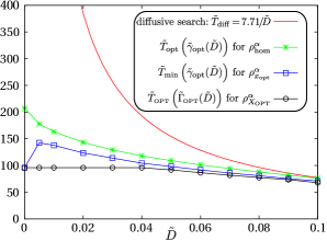
Figure 18: narrow escape, BD; MFPT for purely diffusive search (Eq. 30, red line); search with homogeneously distributed velocity direction (green); search with inhomogeneously distributed velocity direction for the fixed rates $\gamma_{\text{opt}}$, $\gamma^{\prime}_{\text{opt}}=0$ (blue) ; search with inhomogeneously distributed velocity direction for rates $\Gamma_{\text{\textsubscript{\tiny OPT}}}$, $\Gamma^{\prime}_{\text{\textsubscript{\tiny OPT}}}=0$ (black). The points at $\tilde{D}=0$ are based on random velocity direction simulations, as this is the limit for $\tilde{D}\rightarrow 0$.

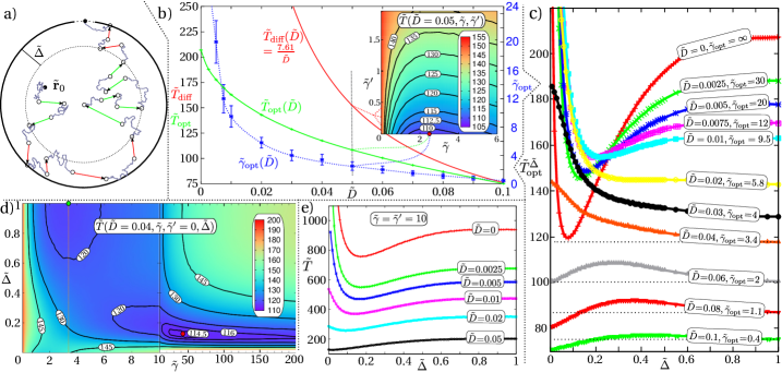
Figure 19: narrow escape, BD, $\rho_{\text{hom}}^{\alpha}$ and $\rho_{p=1,\tilde{D}}^{\alpha}$; a) Sketch of the process with the direction distribution $\rho_{p,\tilde{\Delta}}^{\alpha}$ with a narrow escape region represented by the dotted segment on the surface of the spherical search volume (full black circle). Trajectories of the searcher are represented as in Fig. 3b. b) MFPT for the purely diffusive, ${\tilde{T}}_{\rm diff}$ (red line), and intermittent search, ${\tilde{T}}_{\rm opt}$ (green line), with $\rho_{\text{hom}}^{\alpha}$ and optimal transition rates, as functions of the diffusion constant $\tilde{D}$ for $\vartheta_{\text{abso}}=\text{arcsin(1/7)}$. The optimal rate $\tilde{\gamma}_{\text{opt}}(\tilde{D})$ is represented by the blue line (and right y-axis), ${\tilde{\gamma}^{\prime}}_{\text{opt}}$ vanishes for all $\tilde{D}$. The inset shows as an example for $\tilde{D}=0.05$ a color plot of the MFPT in dependence of the attachment and detachment rates, $\tilde{\gamma}$ and $\tilde{\gamma}^{\prime}$ respectively, the red dot indicates the optimal values (yielding the minimal MFPT) $\tilde{\gamma}_{\text{opt}}(\tilde{D}=0.05)$ and ${\tilde{\gamma}^{\prime}_{\text{opt}}(\tilde{D}=0.05)}$. Optimal attachment / detachment rates like this are used in the main plot for varying diffusion constants. c) MFPT for the inhomogeneous scenario $\rho_{1,\tilde{\Delta}}^{\alpha}$ as a function of $\tilde{\Delta}$ for different diffusion constants $\tilde{D}$ using the optimal rates for the homogeneous scenario. The values at $\tilde{\Delta}=1$ coincide with the data from the blue curve in Fig. b) , as $\rho_{p,\tilde{\Delta}=1}^{\alpha}=\rho_{\text{hom}}^{\alpha}$. d) MFPT as a function of $\tilde{\gamma}$ and $\tilde{\Delta}$ for $\tilde{D}=0.04$, $\tilde{\gamma}^{\prime}=0$. The red dot indicates the global minimum ($\tilde{T}=113.7$) at $\tilde{\gamma}=42$ and $\tilde{\Delta}=0.12$. the green dot (top left) indicates the minimum for the homogeneous case ($\tilde{\Delta}=1$, $\tilde{T}=117.6$). e) MFPT as a function of $\tilde{\Delta}$ for fixed rates $\tilde{\gamma}=\tilde{\gamma}^{\prime}=10$ for different $\tilde{D}$ and $p=1$.

Compared to a purely diffusive searcher (red), an intermittent search strategy with a homogeneous velocity direction distribution (green) optimizes the search process especially for small $\tilde{D}$ significantly, which has already been shown in the inset of Fig. 16. This benefit is even more pronounced than in the case of BB boundary conditions. Again, in the next step, we introduced an inhomoegeneity in the velocity direction distribution (blue), but kept the optimal rate $\tilde{\gamma}$ of the homogeneous case. The additional benefit is much smaller than it was in the BB case, although the total benefit is still larger. In the last step, we varied the transition rate and the degree of inhomoegeneity simultaneously (black). Although the optimal rate again changes dramatically, the additional benefit is as small as in the case of the BB condition.

IV.2.3 inhomogeneous distribution $\rho_{p,\tilde{\Delta}}^{\alpha}$

Fig. 19a) shows a sketch of the class of stochastic first passage processes with direction distribution $\rho_{p,\tilde{\Delta}}^{\alpha}$. The initial position ${\tilde{\mathbf{r}}_{0}}$ of the searcher is now homogeneously distributed within the unit sphere. As already mentioned, the reference time $\tilde{T}_{\text{diff}}$ is expected to decreases slightly by $0.1/\tilde{D}$ and the optimal rates $\tilde{\gamma}_{\text{opt}}$, $\tilde{\gamma}^{\prime}_{\text{opt}}$ are expected to be almost identical to the case of $\tilde{\mathbf{r}}_{0}=0$. Hence, in order to avoid long repetition of almost identical data, the result for the homogeneous scenario is summarized in Fig. 19b): $\tilde{T}_{\text{diff}}(\tilde{D})$ and $\tilde{T}_{\text{opt}}(\tilde{D})$ are almost identical to the corresponding curves of Fig. 18. $\tilde{\gamma}^{\prime}_{\text{opt}}=0$ is also true for a homogeneously chosen initial position, which shows the inset of the plot exemplarily for $\tilde{D}=0.05$ (compare Fig. 12, middle subfigure ) and the values of $\tilde{\gamma}_{\text{opt}}$ are identical (within stochastic fluctuations) to those of Fig. 16.

Similar to the procedure in the sections before, the MFPT for the optimal values of $\tilde{\gamma}_{\text{opt}}(D)$ is now minimized according to the class parameters $p$ and $\tilde{\Delta}$.

Unsurprisingly, $p_{\text{opt}}=1$ holds for all values of $\tilde{D}$. For $p_{\text{opt}}=1$, the dependence of the MFPT on $\tilde{\Delta}$ is shown in Fig. 19c) for different values of $\tilde{D}$. For small values of $\tilde{D}<0.02$, there is always a minimum for $\tilde{\Delta}_{\text{opt}}\in[0.1;0.2]$, i.e. an inhomogeneous strategy is favorable. For $\tilde{D}>0.06$, $\tilde{\Delta}_{\text{opt}}=0$ holds, i.e. the velocity direction of the ballistic motion should always be chosen radially to the outside for all switching positions. For $0.02<\tilde{D}<0.06$ the minimum is at $\tilde{\Delta}=1$, i.e. a homogeneous strategy seems to be optimal in this interval. In order to verify this statement, we varied $\tilde{\gamma}$ and $\tilde{\Delta}$ simultaneously. Exemplarily, the result for $\tilde{\Delta}=0.04$ is shown in Fig. 19d). The dotted line corresponds to the orange ($\tilde{D}=0.04$) curve of subfigure c), i.e. the green dot indicates the minimum at $\tilde{\Delta}=1$. However, there is a global minimum for $\tilde{\Delta}_{\text{OPT}}\approx 0.15$ and $\tilde{\gamma}_{\text{OPT}}\approx 45$, indicated by the red dot. Consequently, the most efficient strategy is again inhomogeneous.

Up to now, we always minimized according to the rates $\tilde{\gamma}$ and $\tilde{\gamma}^{\prime}$ first in order to demonstrate the efficiency of an inhomogeneous strategy afterwards for these optimal rates. In real search, however, these rates might be restricted, for example by an upper value for the allowed energy consumption or the number of available motor proteins in the case of intracellular search. Consequently, systematic studies on the direction distribution for fixed non-optimal rates, motivated by biological data, will also be of interest in further research, but it will go beyond the scope of this publication. However, it should be at least mentioned, that there are robust (here: according to changes in $\tilde{D}$) inhomogeneous strategies, which minimize the MFPT, thus 19e) shows $\tilde{T}$ as a function of $\tilde{\Delta}$ for $\tilde{\gamma}=\tilde{\gamma}^{\prime}=10$ and different values of $\tilde{D}$.

V reaction kinetics

Within this section, the efficiency of intermittent search strategies for an immobile target at the interior of the simulation sphere will be studied. The search process will succeed, if the distance between the diffusive searcher and the target becomes smaller than a reaction distance $d$ for the first time. This introduces a second length scale to the system (in addition to the radius $R$ of the sphere). As the following will stick to the dimensionless units, introduced in the equations (9) and (12), we additionally define

$$\tilde{d}=\frac{d}{R},$$ (32)

which is the reaction distance in the dimensionless units. Within this section we will again study BB and BD boundary conditions for a ballistically moving particle. For the reason of comparison to other publications, we take BB boundary conditions. On the other hand the studies in case of the inhomogeneity $\rho_{p,\tilde{\Delta}}^{\alpha}$ appear more meaningful with BD conditions. But for small $\tilde{d}$ the results differ only very less. Thus the results are almost independent on the applied boundary condition, which is in contrast to the narrow escape problem.
We will study and compare different scenarios for the target position. In subsection V.1 the target is centered in the middle of the simulation sphere and the boundary conditions BB are applied for the reason of comparison. Afterwards, subsection V.2 faces the problem of a homogeneously randomly chosen target position, again with the boundary conditions BB. Finally, in subsection V.3 the scenario of an inhomogeneously distribution of the target position is discussed for the direction distribution $\rho_{p,\tilde{\Delta}}^{\alpha}$ and BD boundary conditions.

V.1 target in the center of the sphere

Due to the radial symmetry of the problem an analytic expression for the reference time $\tilde{T}_{\text{diff}}$ can easily be derived for a searcher, starting at radius $\tilde{r}_{0}>\tilde{d}$ by solving the boundary value problem:

$$\frac{1}{\tilde{r}_{0}^{2}}\frac{\partial}{\partial\tilde{r}_{0}}\left(\tilde{r}_{0}^{2}\frac{\partial}{\partial\tilde{r}_{0}}\tilde{T}_{\text{diff}}(\tilde{d},\tilde{r}_{0})\right)=\frac{-1}{\tilde{D}}\quad\text{ with}\quad\quad$$ (33)

$$T_{\text{diff}}(\tilde{d},\tilde{d})=0\quad\text{and}\quad\frac{\partial}{\partial\tilde{r}_{0}}\tilde{T}_{\text{diff}}(\tilde{d},\tilde{r}_{0})|_{\tilde{r}_{0}=1}=0\;\quad$$ (34)

$$\Rightarrow\quad\tilde{T}_{\text{diff}}(\tilde{d},\tilde{r}_{0})=\frac{-\tilde{d}\tilde{r}_{0}^{3}+\left({2+\tilde{d}^{3}}\right)\tilde{r}_{0}-2\tilde{d}}{6\tilde{D}\tilde{d}\tilde{r}_{0}}\;.\quad\quad\quad$$ (35)

In this section, the initial position of the searcher will always be homogeneously distributed in the spherical shell given by $\tilde{d}<\tilde{r}_{0}<1$. The reference MFPT $\tilde{T}_{\text{diff}}$ of the purely diffusive searcher $\tilde{T}_{\text{diff}}$ will then be given by

$$\tilde{T}_{\text{diff}}(\tilde{d}\hskip 0.56905pt)=\int_{\tilde{d}}^{1}d{\tilde{r}}_{0}\frac{3{\tilde{r}_{0}}^{2}\cdot\tilde{T}_{\text{diff}}(\tilde{d},\tilde{r}_{0})}{1-\tilde{d}^{3}}=\frac{5-9\tilde{d}+5\tilde{d}^{3}-\tilde{d}^{6}}{15\tilde{D}\left({1-{\tilde{d}}^{3}}\right)\tilde{d}}\;.$$ (36)

It is plotted in Fig. 21 (red line). In order to check and prove the accuracy of our numerical method for this scenario we simulated $\tilde{T}_{\text{diff}}$ for $\tilde{d}=0.2$ and $\tilde{d}=0.025$, as these values of $\tilde{d}$ will be used in the following:

$$\tilde{T}_{\text{diff}}(0.2) =\frac{12656}{11625\tilde{D}} \approx\frac{1.08869}{\tilde{D}}$$

$$\tilde{T}_{\text{diff}}^{\text{num}}(0.2) = \frac{1.08857}{\tilde{D}} \quad(10^{7}\text{samples)}$$

$$\tilde{T}_{\text{diff}}(0.025) =\frac{55722849}{4376000\tilde{D}} \approx\frac{12.7337}{\tilde{D}}$$

$$\tilde{T}_{\text{diff}}^{\text{num}}(0.025) = \frac{12.7331}{\tilde{D}} \quad(5\cdot 10^{6}\text{samples)}$$

In both cases the relative deviation is smaller than 0.02 %, which is in the range of the statistical error. We expect the results reported below to have the same numerical accuracy.

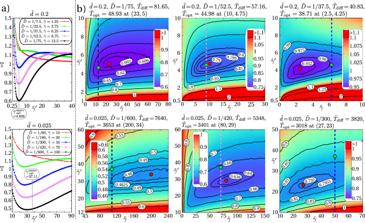
Figure 20: reaction kinetics, $\tilde{\mathbf{r}}_{\text{tar}}=0$, $\rho_{\text{hom}}^{\alpha}$; The upper line shows data for $\tilde{d}=0.2$ ($2\cdot 10^{6}$ samples per data point) , the lower line for $\tilde{d}=0.025$ ($5\cdot 10^{5}$ - $2\cdot 10^{6}$ samples per data point). a) $\mathbb{T}$ as a function of $\tilde{\gamma}^{\prime}$ for different values of $\tilde{D}$ with $\tilde{\gamma}=\tilde{\gamma}_{\text{opt}}^{\text{appro}}=1/(6\tilde{D})$. The dotted gray lines show the position of the suggested minimum $\tilde{\gamma}{{}^{\prime}}^{\text{appro}}_{\text{opt}}$. b) $\mathbb{T}$ is color-coded as a function of $\tilde{\gamma}$ and $\tilde{\gamma}^{\prime}$ for the three smallest values of $\tilde{D}$ in subfigure a). The position of the global minimum $(\tilde{\gamma}_{\text{opt}},\tilde{\gamma}^{\prime}_{\text{opt}})$ is always shown with a red dot. Each colored vertical dotted line corresponds to the curve of subfigure a) in the same color. The green dot shows the position of the proposed optimal rates $\tilde{\gamma}_{\text{opt}}^{\text{appro}},\tilde{\gamma}{{}^{\prime}}^{\text{appro}}_{\text{opt}}$ by Benichou2011 ; Loverdo2008 ; Loverdo2009 .

V.1.1 homogeneous distribution $\rho_{\text{hom}}^{\alpha}$

The studies of Benichou2011 ; Loverdo2008 ; Loverdo2009 already considered the intermittent search problem for the homogeneously distributed velocity direction distribution $\rho_{\text{hom}}^{\alpha}$ and a target centered in the middle of the sphere. Approximating expressions for the transition rates $\gamma_{\text{opt}}$ and $\gamma^{\prime}_{\text{opt}}$ of the search problem were derived there: The dependence of the MFPT $T$ on the rate $\gamma$ is claimed to be very weak and $\gamma_{\text{opt}}^{\text{appro}}=v^{2}/(6D)$ to be a good guess for the optimal switching rate from diffusive to ballistic motion. For the optimal rate from ballistic to diffusive motion, their approximative calculations deliver ${\gamma^{\prime}}_{\text{opt}}^{\text{appro}}=v/(1.078d)$. In the nondimensional coordinates of this article, this relations are transformed to

$$\tilde{\gamma}{{}^{\prime}}^{\text{appro}}_{\text{opt}}=1/(1.078\tilde{d})\quad\text{and}\quad\tilde{\gamma}_{\text{opt}}^{\text{appro}}=1/(6\tilde{D})\;.$$ (37)

The numeric simulations of Benichou2011 ; Loverdo2008 ; Loverdo2009 do not show a simultaneous variation of the two rates, as $\gamma$ is always set to the assumed optimal value $\gamma_{\text{opt}}^{\text{appro}}$.

We now study this scenario more extensively. For the reason of comparison to their results, we investigate the cases $\tilde{d}=0.2$ ($\tilde{D}=$1/7.5, 1/22.5, 1/37.5, 1/52.5, 1/75) and $\tilde{d}=0.025$ ($\tilde{D}=$1/60, 1/180, 1/300, 1/420, 1/600) as these nondimensional values correspond to the geometry parameters of their studies.
Fig. 20a shows $\mathbb{T}$ as a function of $\tilde{\gamma}^{\prime}$ for $\tilde{d}=0.2$ and $\tilde{d}=0.025$ and $\tilde{\gamma}=\tilde{\gamma}_{\text{opt}}^{\text{appro}}$. These results agree with the numerical results of Benichou2011 ; Loverdo2008 ; Loverdo2009 , when rescaling our plots and plotting them in the same manner than the data of their publications. For $\tilde{d}=0.2$ the position of the minimum is in agreement to $\tilde{\gamma}{{}^{\prime}}^{\text{appro}}_{\text{opt}}$. For $\tilde{d}=0.025$ there are already deviations visible. Next, we varied the rates simultaneously. Our simulations confirm the very weak dependence on $\tilde{\gamma}$. Nevertheless, $\tilde{\gamma}_{\text{opt}}$ and $\tilde{\gamma}_{\text{opt}}^{\prime}$ do not seem to scale exactly like predicted in Eq. 37. Fig. 20b show this for the three smallest diffusion coefficients that we have studied for the same values of $\tilde{d}$ as in Fig. 20a. Although $\mathbb{T}_{\text{opt}}$ (red dots) is less than 2$\%$ smaller than the suggested minima (green dots), it is nevertheless stochastically significant enough to claim a deviation in the optimal rates. For small values of $\tilde{D}$, $\tilde{\gamma}_{\text{opt}}$ is larger than $\tilde{\gamma}^{\text{appro}}_{\text{opt}}$, for large values of $\tilde{D}$ it becomes smaller. Furthermore, the optimal value of $\tilde{\gamma}_{\text{opt}}$ seems not to be independent of $\tilde{D}$, as it slightly decreases with increasing diffusivity.
Nevertheless, although the approximations $\tilde{\gamma}{{}^{\prime}}^{\text{appro}}_{\text{opt}}$ and $\tilde{\gamma}_{\text{opt}}^{\text{appro}}$ sometimes differ essentially from simulated minima, they always define a very good search strategy, which is close to the optimal one, as the corresponding MFPT is always very close to $\tilde{T}_{\text{opt}}$.

V.1.2 optimal inhomogeneous distribution of $\rho^{\alpha}$

Similar to the narrow escape problem in section IV, there are more efficient velocity direction distributions than the homogeneous distribution. For a target located in the center of the sphere the optimal intermittent search strategy is obvious: The starting direction of a ballistically moving particle is always chosen to point to the origin, i.e.

$$\rho^{\alpha}(\alpha)=\rho_{p=0,\tilde{\Delta}=0}^{\alpha}=\delta(\alpha-\pi).$$ (38)

For this setup, there are no finite values for $\tilde{\gamma}_{\text{opt}}$ and $\tilde{\gamma}^{\prime}_{\text{opt}}$. As the ballistic motion happens only radially and always directed to the center, it is possible to construct a ballistic motion with target detection. For $\tilde{\gamma}\rightarrow\infty$, $\tilde{\gamma}^{\prime}\rightarrow\infty$ with $\tilde{\gamma}/\tilde{\gamma}^{\prime}\rightarrow 0$ the particle switches infinitely often between diffusion and ballistic motion within every time period. Nevertheless, it moves like a ballistic particle. In consequence, for a fixed starting radius $\tilde{r}_{0}$, we simply get $\tilde{T}(\tilde{r}_{0})=\tilde{r}_{0}-\tilde{d}$. With the help of the Eqs. (35-36) analytic expressions for $\mathbb{T}$ and the break-even value $\tilde{D}_{\text{be}}$ for a switch from a purely diffusive search to an intermittent search (here: ballistic search) can be derived, but will be skipped here.

V.2 homogeneously distributed random target position

The position $\tilde{\bm{r}}_{\text{tar}}$ of the target is homogeneously distributed in a sphere of radius $1-\tilde{d}$. The initial position $\tilde{\bm{r}}_{0}$ of the searcher is homogeneously distributed in the unit sphere with the restriction $||{\bm{r}}_{\text{tar}}-\tilde{\bm{r}}_{0}||>\tilde{d}$. Compared to the situation of a target in the center of the sphere, the reference time $\tilde{T}_{\text{diff}}$ slightly increases and the relative difference increases monotonically with $\tilde{d}$, which can both be seen in Fig. 21.

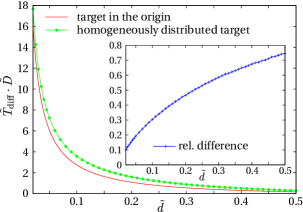
Figure 21: $\tilde{T}_{\text{diff}}\cdot\tilde{D}$ as a function of the reaction distance $\tilde{d}$. Red: Target in the center of the sphere, plot of Eq. 36. Green: Target homogeneously distributed, each green dot is the average value over $2\cdot 10^{6}$ Monte Carlo samples. Blue (inset): relative difference of the green and the red curve.

For the reason of comparison to the subsection before, we analyzed the same parameters $\tilde{d}$ and $\tilde{D}$ as in Fig. 20b. Exemplarily the results for $\tilde{d}=0.2$, $\tilde{D}=1/52.5$ and $\tilde{d}=0.025$, $\tilde{D}=1/420$ are shown in Fig. 22.

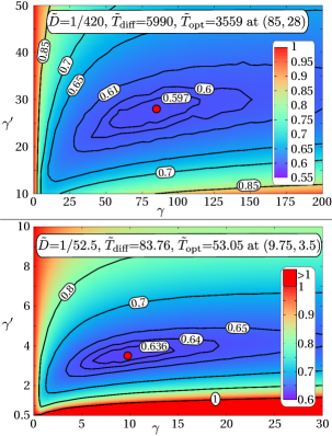
Figure 22: reaction kinetics, ${\tilde{\mathbf{r}}}_{\text{tar}}$ eq. distributed, $\rho_{\text{hom}}^{\alpha}$; $\mathbb{T}$ is color-coded plotted as a function of $\tilde{\gamma}$ and $\tilde{\gamma}^{\prime}$ for the same $\tilde{D}$ and $\tilde{d}$ than in the middle column of Fig. 20b. (top: $\tilde{D}=1/420$, $\tilde{d}=0.025$, bottom: $\tilde{D}=1/52.5$, $\tilde{d}=0.2$). $2-4\cdot 10^{6}$ samples have been done for each data point. The position of the global minimum $(\tilde{\gamma}_{\text{opt}},\tilde{\gamma}^{\prime}_{\text{opt}})$ is always shown with a red dot.

For all investigated cases, the distribution of the target position changes the value of $\tilde{\gamma}_{\text{opt}}(\tilde{D})$ only very less and within the stochastic fluctuations, i.e. $\tilde{\gamma}_{\text{opt}}(\tilde{D})$ seems to depend only on $\tilde{D}$ and $\tilde{d}$. For small values of $\tilde{d}$, this is also true for $\tilde{\gamma}^{\prime}_{\text{opt}}(\tilde{D})$. For larger values of $\tilde{d}$, $\tilde{\gamma}^{\prime}_{\text{opt}}(\tilde{D})$ decreases in the case of a homogeneously distributed target position. Compared to Fig. 20, $\tilde{T}_{\text{opt}}$ is larger for all $\tilde{d}$ and $\tilde{D}$. As this increase is smaller than the increase in $\tilde{T}_{\text{diff}}$, $\mathbb{T}_{\text{opt}}$ decreases. For $\tilde{d}=0.025$ this decrease is only about 7$\%$, for $\tilde{d}=0.2$ it is already about 20 $\%$.

We find that for a homogeneously distributed target position, there is no gain in an inhomogeneously distributed $\rho_{\mathbf{v}}(\Omega|\tilde{\mathbf{r}})$.

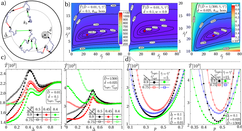
Figure 23: reaction kinetics, ${\tilde{\mathbf{r}}}_{\text{tar}}$ according to $\rho_{w}^{\text{init}}(\tilde{r}_{\text{tar}})$ , $\rho_{\text{hom}}^{\alpha}$ and $\rho_{p,\tilde{\Delta}}^{\alpha}$; a) Sketch of the reaction process for $\rho_{p,\tilde{\Delta}}^{\alpha}$ with an immobile target of diameter $\tilde{d}$ indicated by the gray circle. Trajectories of the mobile particle (searcher), starting at ${\tilde{\bf r}_{0}}$, are represented as in Fig.3b. b) Homogeneous direction distribution: MFPTs as a function of $\tilde{\gamma}$ and $\tilde{\gamma}^{\prime}$ for a spatially homogeneous scenario $\rho_{\text{hom}}^{\alpha}=\rho_{p,1}^{\alpha}$, for (left) $\tilde{D}=0.01,\tilde{d}=0.1$, homogeneously distributed target position $\tilde{\bf r}_{\text{tar}}$; (middle) $\tilde{D}=0.01,\tilde{d}=0.1$, target position $\tilde{\bf r}_{\text{tar}}\leq 0.5$ with probability $w=0.9$; (right) $\tilde{D}=1/300,\tilde{d}=0.025$, homogeneously distributed target position. c) MFPT for the inhomogeneous distribution $\rho_{p,\tilde{\Delta}}^{\alpha}$ with the optimal rates $\tilde{\gamma}_{\text{opt}}(\tilde{D},\tilde{d})$, $\tilde{\gamma}^{\prime}_{\text{opt}}(\tilde{D},\tilde{d})$ from the homogeneous case $\tilde{\Delta}=1$ as function of $\tilde{\Delta}$ for different values of the forward radial transport $p$ and different $w$. d) MFPT as in c) but now with fixed width $\tilde{\Delta}=0.1$ as function of the forward probability $p$ for different fixed rates $\tilde{\gamma}$ and $\tilde{\gamma}^{\prime}$ and different values of $w$.

V.3 inhomogeneously distributed random target position

In the interesting case of a small area where the immobile target is predominantly placed, the best search strategy in not obvious anymore. On the on hand, the searcher should be prevalent in the surrounding of this area. On the other hand, it can’t stay there exclusively, as the target might be somewhere else with a non vanishing probability. This situation shall be studied now for the following distribution of $\tilde{r}_{\text{tar}}=||\tilde{\bm{r}}_{\text{tar}}||$:

$$\rho_{w}^{\text{init}}(\tilde{r}_{\text{tar}})=\left\{{\small\begin{matrix}24w\cdot\tilde{r}_{\text{tar}}^{2}&,&0\leq\tilde{r}_{\text{tar}}\leq\frac{1}{2}\vspace*{0.1cm}\\ \frac{24(1-w)}{8\left({1-\tilde{d}}\right)^{3}-1}\tilde{r}_{\text{tar}}^{2}&,&\frac{1}{2}<\tilde{r}_{\text{tar}}\leq 1-\tilde{d}\vspace*{0.1cm}\end{matrix}}\right.\;,$$ (39)

i.e. with probability $w$, the particle is homogeneously distributed in a sphere of radius $1/2$ around the origin, with probability $1-w$, the particle is homogeneously distributed in the outer region.
The initial position $\tilde{\bm{r}}_{0}$ of the searcher is again homogeneously distributed in the unit sphere with the restriction $||\tilde{\bm{r}}_{\text{tar}}-\tilde{\bm{r}}_{0}||>\tilde{d}$. Fig. 23a) shows a sketch of the resulting stochastic first passage process for the direction distribution $\rho_{p,\tilde{\Delta}}^{\alpha}$. Within this section, we exemplarily study the parameter sets $\tilde{d}=0.1,\tilde{D}=0.01$ and $\tilde{d}=0.025,\tilde{D}=1/300$. Like before, we first face the scenario of a homogeneous search strategy in order to quantify the values of $\tilde{\gamma}_{\text{opt}}$ and $\tilde{\gamma}^{\prime}_{\text{opt}}$. For small values of $\tilde{d}$ these rates are almost independent on $w$, which can be seen by comparing the left and the middle subfigure of Fig. 23b) for $\tilde{d}=0.1$. For $\tilde{d}=0.025$ the differences in the rates totally vanishes within the stochastic fluctuations, hence, only the scenario of a homogeneous initial target position is shown for this case in the right subfigure.

Like before, the influence of the inhomogeneous direction distribution $\rho_{p,\tilde{\Delta}}^{\alpha}$ is studied for the optimal values $\tilde{\gamma}_{\text{opt}}(\tilde{D},\tilde{d})$ and $\tilde{\gamma}^{\prime}_{\text{opt}}(\tilde{D},\tilde{d})$. But due to the computational effort we did not minimize according to $p$ and $\tilde{\Delta}$ in parallel. First, $\tilde{T}$ is minimized according to $\tilde{\Delta}$ for three different values of $p$ for two different $w$. The corresponding plots are shown in Fig. 23c). For $\tilde{d}=0.1$ an inhomogeneous strategy is more efficient for all investigated values of $0.4\leq p\leq 0.5$. For the smaller detection distance $\tilde{d}=0.025$ an inhomogeneous strategy is also preferable, but only in the range of $p\approx 0.5$. Like in the section before, the optimal values of $\tilde{\gamma}_{\text{OPT}}$ and $\tilde{\gamma}_{\text{OPT}}^{\prime}$ in case of an inhomogeneous strategy might strongly differ from $\tilde{\gamma}_{\text{opt}}$ and $\tilde{\gamma}^{\prime}_{\text{opt}}$. We did not calculate the optimal strategy $\tilde{\gamma}_{\text{OPT}}$, $\tilde{\gamma}_{\text{OPT}}^{\prime}$, $p_{\text{OPT}}$, $\tilde{\Delta}_{\text{OPT}}$ explicitly due to the enormous numerical effort of minimizing according to four parameters. Instead Fig. 23d) exemplarily shows the dependence on $p$ for a fixed value of $\tilde{\Delta}=0.1$ for the rates $\tilde{\gamma}_{\text{opt}}(\tilde{D},\tilde{d})$ and $\tilde{\gamma}^{\prime}_{\text{opt}}(\tilde{D},\tilde{d})$ and chosen transition rates. For both $\tilde{d}$ and both values of $w$ the MFPT of the chosen parameters is always beneath the MFPT for $\tilde{\gamma}_{\text{opt}}$, $\tilde{\gamma}^{\prime}_{\text{opt}}$. As already seen in subfigure c), the dependence on $p$ increases for smaller $\tilde{d}$, i.e. the minima are stronger pronounced and the optimal value of $p$ tends to 0.5 (independent on $w$).

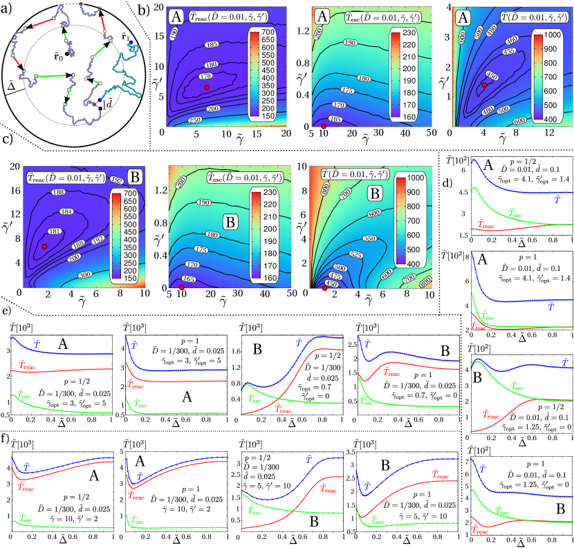
Figure 24: reaction-escape, BD, $\rho_{\text{hom}}^{\alpha}$ and $\rho_{p,\tilde{\Delta}}^{\alpha}$; a) Sketch of the reaction-escape process, involving two particles, an intermittently searching particle (black) and a diffusive target (blue particle), both starting diffusively at random positions $\tilde{\mathbf{r}}_{0}$ and $\tilde{\mathbf{r}}_{1}$. Absorption at the narrow escape region is only possible for searcher-target pair, and the two particles react when coming closer than a distance $\tilde{d}$ and form a pair (brown particle), which will be absorbed at the escape region represented by the dotted segment on the boundary. b) The MFPTs $\tilde{T}_{\text{reac}},\tilde{T}_{\text{esc}}$ and the resulting $\tilde{T}$ are color coded for the homogeneous direction distribution $\rho_{\text{hom}}^{\alpha}$ for situation A and the parameters $\tilde{d}=0.1$ $\tilde{D}=0.01$. c) The MFPTs $\tilde{T}_{\text{reac}},\tilde{T}_{\text{esc}}$ and the resulting $\tilde{T}$ are color coded for the homogeneous direction distribution $\rho_{\text{hom}}^{\alpha}$ for situation B and the parameters $\tilde{d}=0.1$ $\tilde{D}=0.01$. d) The MFPTs $\tilde{T}_{\text{reac}},\tilde{T}_{\text{esc}}$ and the resulting $\tilde{T}$ as a function of $\tilde{\Delta}$ in case of the inhomogeneous direction distributions $\rho_{1/2,\tilde{\Delta}}^{\alpha}$ and $\rho_{1,\tilde{\Delta}}^{\alpha}$ for the situations A and B with parameters $\tilde{d}=0.1$ $\tilde{D}=0.01$ and the optimal transition rates belonging to the corresponding homogeneous direction distribution scenario (position of red dots in the right figures of b) and c) ). e) The MFPTs $\tilde{T}_{\text{reac}},\tilde{T}_{\text{esc}}$ and the resulting $\tilde{T}$ as a function of $\tilde{\Delta}$ in case of the inhomogeneous direction distributions $\rho_{1/2,\tilde{\Delta}}^{\alpha}$ and $\rho_{1,\tilde{\Delta}}^{\alpha}$ for the situations A and B with parameters $\tilde{d}=0.025$ $\tilde{D}=1/300$ and the optimal transition rates belonging to the corresponding homogeneous direction distribution scenario (data not shown). f) The MFPTs $\tilde{T}_{\text{reac}},\tilde{T}_{\text{esc}}$ and the resulting $\tilde{T}$ as a function of $\tilde{\Delta}$ in case of the inhomogeneous direction distributions $\rho_{1/2,\tilde{\Delta}}^{\alpha}$ and $\rho_{1,\tilde{\Delta}}^{\alpha}$ with parameters $\tilde{d}=0.025$ $\tilde{D}=1/300$ and the transition rates $\tilde{\gamma}=10$,$\tilde{\gamma}^{\prime}=2$ (A) , respectively $\tilde{\gamma}=5$,$\tilde{\gamma}^{\prime}=10$ (B).

VI Reaction-Escape Problem

Finally, we study the influence of an inhomogeneous search strategy to a combination of a reaction- and an escape problem for the BD boundary condition. An intermittently searching particle is looking for a mobile particle, which will be found if the searcher and the mobile particle are in the diffusive phase and the particles distance is smaller or equal $\tilde{d}$. Afterwards the particle complex has to solve the narrow escape problem ($\vartheta_{\text{abso}}=\text{arcsin}(1/7)$) (see section IV) with the same search strategy.
AIn the following, two possibilities for the target particle will be studied. In the first case, the target particle moves only diffusively with $\tilde{D}$. Fig. 24a) sketches this situation of the resulting stochastic first passage process for the direction distribution $\rho_{p,\tilde{\Delta}}^{\alpha}$. This scenario is always denoted by situation ”A” in the following. In the second case, there is no difference between the searcher and the target. Both are intermittent searchers. This situation is denoted by ”B”.

The total MFPT $\tilde{T}$ to the escape area at the boundary is the sum of the mean reaction time $\tilde{T}_{\text{reac}}$ and the mean escape time $\tilde{T}_{\text{esc}}$ for the final narrow escape problem:

$$\tilde{T}=\tilde{T}_{\text{reac}}+\tilde{T}_{\text{esc}}\;.$$ (40)

It is no surprise, that we are dealing with a frustrated problem, i.e. the optimal rates for the reaction problem differ from the optimal rates of the narrow escape scenario. Exemplarily Fig. 24b) shows this in case of the homogeneous direction distribution for $\tilde{d}=0.1$, $\tilde{D}=0.01$ in situation A. Furthermore, the optimal rates depend on the considered situation (A or B) , Fig. 24c) shows the same data as subfigure b), but this time for the situation B. However the plots for $\tilde{T}_{\text{esc}}$ (middle in subfigure b) and c), see also Fig. 12 at bottom) are almost identical. The only difference in the investigated narrow escape processes in situation A and B is the distribution of the starting position, as the spatial likelihood of the reaction position differs from A to B. But it has already been shown, that this influence is neglectable for $\vartheta_{abso}=\text{arcsin}(1/7)$. In both situations, for the chosen parameters $\tilde{d}=0.1$ and $\tilde{D}=0.01$ the addends $\tilde{T}_{\text{reac}}$ and $\tilde{T}_{\text{esc}}$ contribute roughly equal to the sum $\tilde{T}_{\text{opt}}$.
Like in the sections before, we now varied $\tilde{\Delta}$ for the optimal rates of the homogeneous scenario for $p=1/2\,,\,1$ in the situations A and B. The four results are shown in Fig. 24d). $\tilde{T}_{\text{reac}}$ is always minimized by an inhomogeneous strategy (especially in situation B). Surprisingly, there is no or almost no a gain in an inhomogeneous strategy for the MFPT $T$, as the MFPT $\tilde{T}_{\text{esc}}$ is always minimized by a homogeneous strategy for the chosen rates.
It raises the question whether an inhomogeneous strategy might be more favorable in scenarios, where $\tilde{T}_{\text{reac}}$ is much larger than $\tilde{T}_{\text{esc}}$. For answering it, we decreased $\tilde{d}$ and investigated the parameters $\tilde{D}=1/300$, $\tilde{d}=0.025$. First, the optimal rates of the homogeneous scenario were determined in the situations A and B. As the corresponding figures qualitatively look like Fig. 24b) and c), these plots are skipped here. Similar to the parameter set before, we now varied $\tilde{\Delta}$ for these optimal rates of the homogeneous scenario for $p=1/2\,,\,1$ in the situations A and B, the result is shown in 24e). In situation A, there is again no or only little gain in an inhomogeneous strategy. For B, there is an enormous gain for p=1/2, and a small one for p=1.
Due to the number of simulations, we did not minimize the rates $\tilde{\gamma},\tilde{\gamma}^{\prime}$ and the inhomoegeneity parameters $p$ and $\tilde{D}$ simultaneously. Instead, in Fig 24f) we show examples for the variation of $\tilde{\Delta}$ for rates, which do not optimize the homogeneous scenario. In all cases, the MFPT for small $\tilde{\Delta}$ is significantly less than in the homogeneous scenario ($\tilde{\Delta}=1$). For p=1 in situation B, the value of the inhomogeneous minimum is even a little bit smaller than the optimal value of the scenario with the rates $\tilde{\gamma}_{\text{opt}}$ and $\tilde{\gamma}_{\text{opt}}$, compare right figures of subfigure e) and f) . In consequence, the optimal strategy is for sure also an inhomogeneous one, at least in this scenario.

VII Summary

In this work we have studied the efficiency of spatially homogeneous and inhomogeneous intermittent search strategies for three paradigmatic search problems in spheres: narrow escape problem, reaction kinetics and the reaction-escape problem. Our results are obtained by an event driven Monte Carlo algorithm, which has recently been published schwarz2013 . The working horses of this algorithm are sampling routines which depend on the geometry of the search domain under consideration. We developed highly efficient sampling routines for spherical domains, which are much faster than routines published so far. Since the potential applications of these routines are universal in the field of First Passage Kinetic Monte Carlo algorithms, they are explained in the appendix in detail.

Before summarizing each of the three search problems individually, some general remarks, relevant for all studied scenarios, are in appropriate::
The break-even diffusivity $\tilde{D}_{\text{be}}$ (the value of $\tilde{D}$ where the best strategy changes from intermittent to purely diffusive search) increases with the target size $s\in\{\vartheta_{\text{abso}}$, $\tilde{d}\}$. Consequently, if intermittent search is the best strategy, the fraction of time spend in the diffusive mode will be monotonically increasing in $\tilde{D}$ and decreasing in $s$.
For small targets, the MFPT does almost not depend on the distribution of the initial position $\mathbf{r}_{0}$ or the initial mode (diffusive or ballistic), as the time for the searcher to lose its memory about the initial position is much shorter than the MFPT.
Furthermore, we observed, that the MFPT $\tilde{T}$ as a function of the transition rates $\tilde{\gamma}$ and $\tilde{\gamma}^{\prime}$ seems always to be convex. However, the positions of the minima $(\tilde{\gamma}_{\text{opt}},\tilde{\gamma}^{\prime}_{\text{opt}})$ and $(\tilde{\Gamma}\text{\textsubscript{\tiny OPT}},\tilde{\Gamma}^{\prime}\text{\textsubscript{\tiny OPT}})$ are never sharp, neither in $\tilde{\gamma}$, nor in $\tilde{\gamma}$, which can be seen by comparing the values of neighbored isolines in the color coded plots. Hence, in a quite large surrounding (relative to the absolute values), the MFPT $\tilde{T}$ is only slightly larger than the optimal value. This is remarkable for real search, as this fact offers the opportunity to optimize the search process also according to other criteria (e.g. energy consumption or usage of limited resources, for instance fuel necessary for ballistic motion, like ATP for motor proteins in the biological context) without increasing the MFPT significantly.
For the inhomogeneous search strategies that we studied, the behavior of the MFPT as a function of the inhomogeneity parameters $x$ and $(p,\tilde{\Delta})$ sometimes differs. Especially for small diffusion constants $\tilde{D}$ and a large transition rate $\tilde{\gamma}$, the optimal searching strategy depends strongly on the chosen inhomogeneity parameters. In addition, more than one local minimum of $\tilde{T}$ might occur in dependence of the tunable parameters (see Fig. 19d).
The dependence on the applied boundary conditions at the border of the searching domain varies strongly in the scenarios that we analyzed. If the target is predominantly located very close (compared to $1/\tilde{\gamma}^{\prime}$ $\hat{=}$ average covered distance in the ballistic state ) to the boundary or even part of it (narrow escape problem), the MFPT and the optimal strategy will strongly be influenced by the boundary condition. If $\tilde{\gamma}^{\prime}$ and/or the average distance from the target to the boundary increases, this influence shrinks rapidly.

The first search scenario that we considered is the so called narrow escape problem. It is well understood for a purely diffusive particle, but apart from schwarz2016 there are no studies for intermittent search available in literature. Thus, before studying inhomogeneous strategies, we analyzed first the homogeneous scenarios for the reason of comparison. The value of the break-even diffusivity $\tilde{D}_{\text{be}}$ depends strongly on the considered boundary conditions. For the exemplarily chosen small opening angle $\vartheta_{\text{abso}}=$arcsin(1/7) it is about 4 times smaller for the BB (ballistic-ballistic) boundary condition ($\tilde{D}_{\text{be}}\approx 0.025$) than for the BD (ballistic-diffusive) scenario ($\tilde{D}_{\text{be}}\approx 0.1$). Furthermore, there is a qualitative difference in the behaviour of the optimal transition rates $\tilde{\gamma}_{\text{opt}}$ and $\tilde{\gamma}^{{}^{\prime}}_{\text{opt}}$ as a function of $\tilde{D}<\tilde{D}_{\text{be}}$. For the BB boundary condition, the optimal transition rates both decrease with $\tilde{D}$. For BD, only $\tilde{\gamma}_{\text{opt}}(\tilde{D})$ decreases, while $\tilde{\gamma}^{{}^{\prime}}_{\text{opt}}(\tilde{D})=0$ holds for all $\tilde{D}$. Thus, it is always part of the best strategy to end the ballistic phase only when being forced by the BD condition at the boundary of the simulation sphere. As $\tilde{\gamma}^{{}^{\prime}}_{\text{opt}}$ vanishes for all $\vartheta_{\text{abso}}$, the numerical effort for finding the best strategy is essentially reduced. Hence, in addition to $\tilde{D}$, we also varied $\vartheta_{\text{abso}}$ systematically. Fig. 15 (in combination with the nondimensionalisation relations) offers a full numeric solution for the best homogeneous search strategy in the BD case as a function all parameters, which is the diffusivity $D$, the radius $R$, the velocity $v$ (ballistic mode) and the target area with polar angle $\vartheta_{\text{abso}}$.
For both boundary conditions, the MFPT can be significantly reduced by the usage of inhomogeneous searching strategies, which has been shown for the direction distributions $\rho_{x}^{\alpha}$ and $\rho_{p,\tilde{\Delta}}^{\alpha}$. The family $\rho_{x}^{\alpha}$ has exclusively been designed by us for optimizing the narrow escape problem, it is not efficient for targets at the interior of the searching domain. Surprisingly, for the rates $\tilde{\gamma}_{\text{opt}}$ and $\tilde{\gamma}^{{}^{\prime}}_{\text{opt}}$ the optimal strategies of the biologically inspired family $\rho_{p,\tilde{\Delta}}^{\alpha}$ can almost compete with the results of $\rho_{x}^{\alpha}$ for small $\tilde{D}$, which can be seen by comparing the values of $\tilde{T}_{\text{min}}$ in Table 2 with the minima of Fig. 19c). This is remarkable, as $\rho_{p,\tilde{\Delta}}^{\alpha}$ was not specially designed for the narrow escape problem and is also a good strategy for the other search scenarios.
Furthermore, the optimal transition rates depend strongly on the considered direction distribution (up to a factor of 10) in all investigated scenarios, which can be seen by comparing $\tilde{\gamma}_{\text{opt}}$ vs $\tilde{\Gamma}_{\text{OPT}}$, $\tilde{\gamma}^{{}^{\prime}}_{\text{opt}}$ vs $\tilde{\Gamma}^{{}^{\prime}}_{\text{OPT}}$ in the Tables 1, 2 and the $\tilde{\gamma}$-coordinates of the homogeneous and inhomogeneous minima in Fig. 19d).

Next, we focused on the problem an immobile target in the interior of the sphere, called reaction kinetics. For a target at the origin, it has been shown that the analytic approximations of Benichou2011 ; Loverdo2008 ; Loverdo2009 for the optimal rates $\tilde{\gamma}_{\text{opt}}$ and $\tilde{\gamma}^{\prime}_{\text{opt}}$ slightly (but systematically) differ from the minima position. Nevertheless, these approximations define almost perfect searching strategies, as the MFPT is almost nearly insensitive to a variation of the rates in quite a large surrounding of the optimal values.
In case of a homogeneous searching strategy, the influence of the distribution of the target position is rather small. If the target position is homogeneously randomly chosen, $\tilde{T}_{\text{diff}}$ and $\tilde{T}_{\text{opt}}$ slightly increase compared to a centered target. Nevertheless, for small target sizes the optimal transition rates $\tilde{\gamma}_{\text{opt}}$ and $\tilde{\gamma}^{\prime}_{\text{opt}}$ turned out to be independent of the target distribution within the sphere. For larger target sizes $\tilde{\gamma}_{\text{opt}}$ remains independent, only $\tilde{\gamma}^{\prime}_{\text{opt}}$ slightly increases in the cases that we investigated. Furthermore, if there is no predominantly chosen target position, a homogeneous searching strategy will be the optimal solution.
Things change, when the immobile target is predominantly (but not exclusively) placed in a specific area. Within the family $\rho_{p,\tilde{\Delta}}^{\alpha}$ there are inhomogeneous strategies which are essentially more efficient than a homogeneous one (Fig. 23).

Finally, we considered the combination of two search processes, called reaction-escape problem. An intermittently searching particle has first to find an either purely diffusive (A) or also intermittently moving particle (B) before finding a narrow escape. Dealing with a frustrated problem, the optimal rates for the MFPT $\tilde{T}_{\text{reac}}$ of the particle-particle binding differ from the optimal rates of the narrow escape problem $\tilde{T}_{\text{esc}}$. In consequence, the overall optimal strategy, i.e. transition rates which minimize $\tilde{T}=\tilde{T}_{\text{reac}}+\tilde{T}_{\text{esc}}$ are a compromise in between. Depending on the ratio of the absolute values of $\tilde{T}_{\text{reac}}$ and $\tilde{T}_{\text{esc}}$ (mostly controlled via the size of the reaction distance $\tilde{d}$ in comparison to the opening angle $\vartheta_{\text{abso}}$), the total influence on the best strategy varies.
The gain of an inhomogeneous searching scenario depends strongly on the investigated parameters and states of motion for the target particle (A or B). However, there is a large parameter regime in which an inhomogeneous searching strategy is most efficient.

To conclude we have demonstrated the efficiency of spatially inhomogeneous search strategies, which were introduced by us recently schwarz2016 . The space of possible spatial inhomogeneities is large and we confined our study only to two parameterized families of search strategies, which already turned out to be more efficient than homogeneous strategies. Most probably even more efficient strategies exist outside the families studied here, and it would be highly desirable to explore the space of possible strategies, in particular direction distributions, with alternative, possibly more powerful tools than brute force numerical studies. Currently the quest for the optimal inhomogeneous search strategy remains a challenge for future work. Potential applications comprise the spatial organization of cytoskeleton in living cells schwarz2016 , but also the wide field of search in spatially inhomogeneous domains and/or with spatially inhomogeneous target distributions.

Acknowledgement

This work was financially supported by the German Research Foundation (DFG) within the Collaborative Research Center SFB 1027.

Appendix A Fast generation of random numbers

Based on the Green’s functions $P_{S}$ (sphere) and $P_{C}$ (cone) for a diffusive particle starting at the origin of a sphere or spherical cone with polar angle $\Theta$ ($0\leq\vartheta\leq\Theta$) respectively, this appendix presents efficient methods for sampling the occurring densities, needed within the simulations of this paper, in detail:

• probability density for reaching the absorbing radius $R_{pro}$ of a sphere/cone for the first time at time $t$ at an arbitrary solid angle when starting at the origin.

• probability density for being at radius $r$ within a sphere/cone at time $t$ at an arbitrary solid angle under the condition of not having reached radius $R_{pro}$ before and having started at the origin.

Due to the radial symmetry of these problems, the density of the solid angle is homogeneously distributed on the surface of either a sphere or a spherical cone for all $t$ and $r\in[0;R_{pro}]$. Thus its sampling in case of a position update can be done very fast, which is among others shown in chapter V. 4 of devroye1986 .
In the following, the index ”$pro$” is skipped at the radius $R_{pro}$. It shortens the notation and there is no danger of mixing it up with the radius of the simulation sphere within this appendix.
Although ways of sampling the densities $\rho_{b}$, $\rho_{n}$ have already been published in donev2010 , we want to present significantly faster methods to sample them by picking up their idea (donev2010 ) of different representations for large and small times, but avoiding their bottleneck: the numerical inversion of cumulative distribution functions, which results in the calculation of many exponential and trigonometrical functions, slowing the algorithm down. Especially a fast sampling of $\rho_{b}$ is very important as a random number according to this distribution is always needed after the creation of a protection sphere/cone, which is part of the innermost loop of the simulation.

A.1 The analytic solutions $P_{S}$ and $P_{C}$ of the diffusion equation

A.1.1 The sphere

The diffusion problem within a totally absorbing sphere of radius $R$ is given by

$$\frac{\partial{P(r,\varphi,\vartheta,t)}}{\partial{t}} = D\Delta P(r,\varphi,\vartheta,t)\;,\text{ with}$$ (41)

$$P(R,\varphi,\vartheta,t) = 0\;\;\;\forall\;\varphi\in[0;2\pi[,\vartheta\in[0;\pi]\;.$$

In carslaw1959 the solution for a particle at an arbitrary starting radius $r_{0}<R$ is derived. With the help of l’Hospital’s rule ($r_{0}\rightarrow 0$) the following expression for the radial symmetric probability density $P_{S}$ can be obtained:

$$P_{S}(r,t)=\frac{1}{2R^{2}r}\sum_{n=1}^{\infty}e^{-\pi^{2}n^{2}\frac{Dt}{R^{2}}}\,n\,\sin\left(\frac{n\pi r}{R}\right)\;.$$ (42)

For the sake of computational efficiency it is useful to derive a second expression for $P_{S}$ by applying Poisson’s summation formula to Eq. (42).

$$P_{S}(r,t)=\frac{1}{8\left(\pi Dt\right)^{\frac{3}{2}}}\,\times\hskip 128.0374pt$$ (43)

$$\hskip 5.69054pt\left\{e^{\frac{-r^{2}}{4Dt}}+\sum_{k=1}^{\infty}\left(\frac{2kR+r}{r}e^{\frac{-(2kR+r)^{2}}{4Dt}}-\frac{2kR-r}{r}e^{\frac{-(2kR-r)^{2}}{4Dt}}\right)\right\}$$

For large $t$ the series of Eq. (42) converges very fast, whereas for small $t$ the series of Eq. (43) does.

A.1.2 The spherical cone

The diffusion problem within a spherical cone of radius $R$ and polar angle $\Theta$, reflecting at the conical boundary and absorbing at the spherical cap is given by

$$\frac{\partial{P(r,\varphi,\vartheta,t)}}{\partial{t}} = D\Delta P(r,\varphi,\vartheta,t),\;\;\text{with}$$ (44)

$$P(R,\varphi,\vartheta,t) = 0\;\;\;\forall\;\varphi\in[0;2\pi[,\vartheta\in[0;\Theta]\;,$$

$$\left.\frac{\partial{P(r,\varphi,\vartheta,t)}}{\partial{\vartheta}}\right|_{\vartheta=\Theta} = 0\;\;\;\forall\;r\in[0;R],\varphi\in[0;2\pi[\;.$$

In the general case of an arbitrary starting position, its solution looks very complex, but for the case of interest ($r_{0}=0$), we simply obtain a radial symmetric probability density, which is proportional to the solution of the subsection above:

$$P_{C}(r,t)=\frac{2}{1-\cos(\Theta)}P_{S}(r,t)$$ (45)

A.2 The probability densities $\rho_{b}(t)$, $\rho_{n}(r|t)$

Based on the formulas (42) and (43), two different expressions for each of the probability densities $\rho_{b}$ and $\rho_{n}$ can be derived. The upper index “$>$” will always mark the series, which converges fast for large $t$, while the upper index “$<$” will mark the series, which converges fast for small $t$. If there is no upper index, it is a general statement, i.e. independent of the series representation. The probability density $\rho_{b}(t)$ is identical for the sphere and the cone of radius $R$ and given by

$$\rho_{b}(t) = -\frac{d}{dt}\left[\int_{0}^{R}dr\int_{0}^{2\pi}d\varphi\int_{0}^{\pi}d\vartheta\,r^{2}\sin(\vartheta)\,P_{S}(r,t)\right]\quad\quad$$

$$= -\frac{d}{dt}\left[\int_{0}^{R}dr\int_{0}^{2\pi}d\varphi\int_{0}^{\Theta}d\vartheta\,r^{2}\sin(\vartheta)\,P_{C}(r,t)\right]\;.$$

Applying this to the series (42) and (43), we get:

$$\rho_{b}^{>}(t) = \frac{2\pi^{2}D}{R^{2}}\sum_{n=1}^{\infty}e^{-\pi^{2}n^{2}\frac{Dt}{R^{2}}}(-1)^{n+1}n^{2}\;,$$

$$\rho_{b}^{<}(t) = \frac{R^{3}}{2\sqrt{\pi D^{3}t^{5}}}\sum_{k=1}^{\infty}e^{-\frac{R^{2}(2k-1)^{2}}{4Dt}}\left((2k-1)^{2}-2\frac{Dt}{R^{2}}\right)\;.$$

The probability density $\rho_{n}(r|t)$ is also identical for the sphere and the cone of radius $R$ and given by

$$\rho_{n}(r|t) = \dfrac{\int_{0}^{2\pi}d\varphi\int_{0}^{\pi}d\vartheta\,r^{2}\sin(\vartheta)\,P_{S}(r,t)}{\int_{0}^{R}dr\int_{0}^{2\pi}d\varphi\int_{0}^{\pi}d\vartheta\,r^{2}\sin(\vartheta)\,P_{S}(r,t)}$$

$$= \dfrac{\int_{0}^{2\pi}d\varphi\int_{0}^{\Theta}d\vartheta\,r^{2}\sin(\vartheta)\,P_{C}(r,t)}{\int_{0}^{R}dr\int_{0}^{2\pi}d\varphi\int_{0}^{\Theta}d\vartheta\,r^{2}\sin(\vartheta)\,P_{C}(r,t)}\;.$$

In consequence, we get:

$$\rho_{n}^{>}(r|t) = \frac{\pi r}{R^{2}}\dfrac{\sum\limits_{n=1}^{\infty}e^{-\pi^{2}n^{2}\frac{Dt}{R^{2}}}n\sin\left(\frac{n\pi r}{R}\right)}{\sum\limits_{n=1}^{\infty}e^{-\pi^{2}n^{2}\frac{Dt}{R^{2}}}(-1)^{n+1}}\;,\hskip 142.26378pt$$

$$\rho_{n}^{<}(r|t) =$$

$$\dfrac{r^{2}e^{\frac{-r^{2}}{4Dt}}+r\sum\limits_{k=1}^{\infty}\left((2kR+r)e^{\frac{-(2kR+r)^{2}}{4Dt}}-(2kR-r)e^{\frac{-(2kR-r)^{2}}{4Dt}}\right)}{2Dt\left(\sqrt{\pi Dt}-2R\sum\limits_{k=1}^{\infty}e^{-\frac{R^{2}(2k-1)^{2}}{4Dt}}\right)}\;.$$

A.3 Efficient sampling of $\rho_{b}(t)$

Instead of designing a sampling routine including the parameters $R$ and $D$, it is computationally more efficient to sample the dimensionless random number

$$\tau=\frac{D}{R^{2}}t\;,$$

as $R^{2}/D$ is the characteristic timescale. For its probability density $\tilde{\rho}_{b}$, we get

$$\tilde{\rho}_{b}(\tau)=\frac{R^{2}}{D}\,\,\rho_{b}\left(\frac{R^{2}}{D}\tau\right)\;,$$

which leads to the following series representations

$$\tilde{\rho}_{b}^{>}(\tau) = 2\pi^{2}\sum_{n=1}^{\infty}e^{-\pi^{2}n^{2}\tau}\left(-1\right)^{n+1}n^{2}$$ (48)

$$\tilde{\rho}_{b}^{<}(\tau) = \frac{1}{2\sqrt{\pi\tau}\tau^{2}}\sum_{k=1}^{\infty}e^{-\frac{(2k-1)^{2}}{4\tau}}\left(\left(2k-1\right)^{2}-2\tau\right)\,\,.\quad\quad$$ (49)

The corresponding distribution function can be expressed via the Jacobi-Theta function $\vartheta_{4}$:

$$\tilde{F}_{b}(\tau)=\vartheta_{4}\left(0,e^{-\pi^{2}\tau}\right)\;.$$

Although this function is well studied in mathematics, there seems to be no way to invert it analytically. In consequence, sampling via the Inversion method would require a numerical inversion tool, which slows the algorithm dramatically down.

Hence, we decided to use a fast way of rejection sampling, which is described below:

Depending on the needed numerical accuracy, the questions of where to truncate the sums (48) , (49) and when to switch between these two representations has to be answered. With the following choice one is on the safe side for all practical purposes:

$$\tilde{\rho}_{b}^{\text{num}}(\tau)=\left\{{\small\begin{matrix}2\pi^{2}\sum\limits_{n=1}^{n_{\text{max}}(\tau)}e^{-\pi^{2}n^{2}\tau}\left(-1\right)^{n+1}n^{2}&,&\tau\geq\tau_{c}\vspace*{0.2cm}\\ \frac{1}{2\sqrt{\pi\tau}\tau^{2}}\sum\limits_{k=1}^{k_{\text{max}}(\tau)}e^{-\frac{(2k-1)^{2}}{4\tau}}\left(\left(2k-1\right)^{2}-2\tau\right)&,&\tau<\tau_{c}\end{matrix}}\right.\;.$$

with $\tau_{c}=0.25$ and the piece-wise constant integer functions

$$n_{\text{max}}(\tau)=\left\{{\small\begin{matrix}4&,&\tau\in\left[0.25;0.3\right[\vspace*{0.1cm}\\ 3&,&\tau\in\left[0.3;0.6\right[\vspace*{0.1cm}\\ 2&,&\tau\in\left[0.6;1.5\right[\vspace*{0.1cm}\\ 1&,&\tau\in\left[1.5;\infty\right[\end{matrix}}\right.\;,$$

$$k_{\text{max}}(\tau)=\left\{{\small\begin{matrix}3&,&\tau\in\left[0.125;0.25\right[\vspace*{0.1cm}\\ 2&,&\tau\in\left[0.04;0.125\right[\vspace*{0.1cm}\\ 1&,&\tau\in\left]0;0.04\right[\end{matrix}}\right.\;.$$

Using this choice, the relative deviation fulfills

$$\frac{|\tilde{\rho}_{b}(\tau)-\tilde{\rho}_{b}^{\text{num}}(\tau)|}{\tilde{\rho}_{b}(\tau)}<10^{-18}\;\;\forall\;\tau>0\;,\text{i.e.}$$

we never have to add more than four addends to calculate $\tilde{\rho}_{b}(\tau)$ within double precision.

For using rejection sampling, a helping probability density $\rho_{h}(\tau)$ and a scaling constant $k>1$ (as small as possible) with $k\geq\frac{\tilde{\rho}_{b}(\tau)}{\rho_{h}(\tau)}\;\forall\;\tau$ have to be found devroye1986 . Furthermore there must be the possibility to generate random numbers according to $\rho_{h}(\tau)$ very fast. For these purposes we divide $\mathbbm{R}^{+}_{0}$ into $N$ intervals $[\tau_{i},\tau_{i+1}[$ with $\tau_{0}=0$ and $\tau_{N}=\infty$. For the first $N-1$ intervals we want $\rho_{h}(\tau)$ to be piece-wise constant:

$$\rho_{h}(\tau)=\frac{p_{i}}{k}\quad\forall\;\tau\in[\tau_{i},\tau_{i+1}]\;,\;i\in\left\{0,...,N-2\right\}\;,\quad\quad$$ (50)

with $p_{i}=\operatorname*{\text{max}}\limits_{[\tau_{i},\tau_{i+1}]}\tilde{\rho}_{b}(\tau)$. Having chosen the length of the first interval $[\tau_{0},\tau_{1}]$, we define a constant $Q=(\tau_{1}-\tau_{0})\cdot p_{0}$ and the length of all the other intervals is determined via

$$(\tau_{i+1}-\tau_{i})\cdot p_{i}=Q\quad\;\forall\;i\in\left\{1,...,N-2\right\}\;.$$ (51)

These calculations cannot be done in a straightforward manner, as $p_{i}$ is also a function of $\tau_{i+1}$. Nevertheless it is possible to iterate it as exact, as wanted (more than double precision) by using floating data-types with an arbitrary exactness. Since the calculation of all $\tau_{i}$ and $p_{i}$ have to be done once only, in order to include them in our implementation, we don’t have to care about the running time of it.

For the tail interval $[\tau_{N-1};\infty[$ we choose $\rho_{h}(\tau)=\frac{Q}{k(\tau+1-\tau_{N-1})^{2}}$. Thus, the cumulative probability of each interval is the same: $Q/k$. Keeping in mind, that there are $N$ intervals, we get:

$$k=N\cdot Q\;,$$ (52)

and in consequence:

$$\rho_{h}(\tau) = \left\{{\small\begin{matrix}\frac{p_{0}}{k}&,&\tau\in[\tau_{0};\tau_{1}[\vspace*{0.1cm}\\ \frac{p_{1}}{k}&,&\tau\in[\tau_{1};\tau_{2}[\vspace*{0.1cm}\\ \vdots&&\vdots\\ \frac{p_{N-2}}{k}&,&\tau\in[\tau_{N-2};{\tau_{N-1}}[\vspace*{0.1cm}\\ \frac{1}{N(\tau+1-\tau_{N-1})^{2}}&,&\tau\geq\tau_{N-1}\end{matrix}}\right.\;.\quad\quad\quad$$ (53)

An illustration of this procedure for a rather rough $\rho_{h}$ by choosing $\tau_{1}=0.038$ ($\rightarrow N=25$) and the case of $\tau_{1}=0.025$ ($\rightarrow N=332$), which was used in our simulations is shown in Fig. 25.

Figure 25: Illustration for the construction of $\rho_{h}(\tau)$ for the cases $\tau_{1}=0.038$ ($\rightarrow N=25$) and $\tau_{1}=0.025$ ($\rightarrow N=332$). The case N=25 is created only to clarify the construction mechanism. The case N=332 is used in our implementation.

The corresponding distribution function is given by

$$F_{h}(\tau)=\left\{{\small\begin{matrix}\frac{p_{0}}{k}\tau&,&\tau\in[\tau_{0};\tau_{1}[\\ \frac{1}{N}+\frac{p_{1}}{k}(\tau-\tau_{1})&,&\tau\in[\tau_{1};\tau_{2}[\\ \frac{2}{N}+\frac{p_{2}}{k}(\tau-\tau_{2})&,&\tau\in[\tau_{2};\tau_{3}[\\ \vdots&&\vdots\\ \frac{N-2}{N}+\frac{p_{N-2}}{k}(\tau-\tau_{N-2})&,&\tau\in[\tau_{N-2};\tau_{N-1}[\\ 1-\frac{1}{N(\tau+1-\tau_{N-1})}&,&\tau\geq\tau_{N-1}\end{matrix}}\right.$$ (54)

As every interval has the same probability mass $1/N$, a random number $\tau_{\text{cand}}$ according to $\rho_{h}$ can be generated very fast, as $F_{h}$ can be inverted very fast straightforwardly without the usage of a bisection method:
The integer number $m\in\left\{0,...,N-1\right\}$, given by

$$m=\lfloor r_{\text{cand}}\cdot N\rfloor\;,$$ (55)

immediately indicates the candidate’s interval $[\tau_{m};\tau_{m+1}]$ of $F_{h}(\tau)$, where $r_{\text{cand}}$ is a random number from a uniform distribution in the interval $]0,1[$. Solving for $\tau$ in the $m$-th interval of Eq. (54) yields

$$\tau_{\text{cand}}=\left\{{\small\begin{matrix}\left(r_{\text{cand}}-\frac{m}{N}\right)\cdot\frac{k}{p_{m}}+\tau_{m}&,&m\in\left\{0,...,N-2\right\}\\ \tau_{N-1}-1+\frac{1}{N(1-r_{\text{cand}})}&,&m=N-1\end{matrix}}\right..\quad\quad$$ (56)

The choice of $\tau_{1}=0.025$ for the construction of $\rho_{h}(\tau)$ (see Fig. 25) results in $Q=0.003078...$, $N=332$ and $k=1.02...\,$. In consequence we are dealing with a very efficient way of rejection sampling, as the rejection rate is about 2 $\%$.
Nevertheless it is possible to improve this sampling significantly by having a closer look at the procedure of rejection sampling: At first, a candidate random number $\tau_{\text{cand}}$ according to $\rho_{h}(\cdot)$ is chosen. As explained above, this is possible very fast. $\tau_{\text{cand}}$ is accepted, if the quotient $\tilde{\rho}_{b}(\tau_{\text{cand}})/(k\rho_{h}(\tau_{\text{cand}}))$ is bigger than a uniformly distributed random number $r_{\text{rej}}$ in the interval $[0;1]$. Using the method above, this happens in around $1/k\approx 98$ $\%$ of the cases. The most time consuming part is the calculation of $\rho_{b}(\tau_{\text{cand}})$, as it includes 1-4 addends. This calculation can often be avoided by formulating one (or more) precondition for acceptance: About 90$\%$ of the $\tau_{\text{cand}}$ will be in the interval $[0.05;0.354]$. There the quotient $\tilde{\rho}_{b}/(k\,\rho_{h})$ is bigger than 0.95 everywhere, which is illustrated in Fig. 26

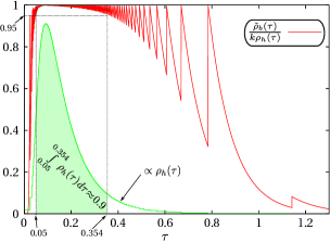
Figure 26: $\tilde{\rho}_{b}(\tau)/(k\,\rho_{h}(\tau))$: Around 90 $\%$ of all random numbers $\tau_{\text{cand}}$ will be produced in the interval $[0.05;0.354]$. The ratio $\tilde{\rho}_{b}/(k\,\rho_{h})$ is bigger than 0.95 within this interval.

Hence, for $r_{\text{rej}}<0.95$, we can accept without evaluating $\tilde{\rho}_{b}$. In consequence, only in $1-0.95\cdot 0.9\approx 15$ $\%$ of the cases we really have to evaluate $\tilde{\rho}_{b}$. This fraction can be further reduced by formulating more preconditions for $\tau<0.05$ and $\tau>0.354$. But the gain won’t be large, as already 90$\%$ of the $\tau_{\text{cand}}$ are covered.
Let’s summarize the average effort: Per candidate $\tau_{\text{cand}}$ we need only one equally distributed random number $r_{\text{cand}}$ and 6 trivial operations ($+,-,\cdot,/$) for the calculations of the Eqs. (55, 56). The rejection rate $\frac{k-1}{k}$ is only about 2 $\%$ and the computational price for the acceptance decision is the generation of an equally distributed random number $r_{\text{rej}}$ and on average less than 0.5 addends in the formulas (48), (49). A C++-implementation of the described method on a single CPU-core with 3.4 GHz takes around 35 sec for $10^{9}$ random $\tau$. About 14 sec of this time have been used to generate high quality uniformly distributed random numbers for $r_{\text{cand}}$ and $r_{\text{rej}}$ with the help of the gsl routine “gsl_rng_mt19937” based on the Mersenne Twister mersenne1998 .

A.4 Efficient sampling of $\rho_{n}(r|t)$

In addition to the characteristic time scale, we want to use the characteristic length scale $R$ and define the dimensionless length

$$x=\frac{1}{R}r\quad.$$ (57)

For its probability density, we get:

$$\tilde{\rho}_{n}(x|\tau)=R\rho_{n}\left(xR\left|\frac{R^{2}}{D}\tau\right.\right)\;,$$

which leads to the following series representations

$$\tilde{\rho}_{n}^{>}(x|\tau) = \pi x\dfrac{\sin\left(\pi x\right)+\sum\limits_{n=2}^{\infty}e^{-\pi^{2}\left(n^{2}-1\right)\tau}n\sin\left(n\pi x\right)}{1-\sum\limits_{n=2}^{\infty}e^{-\pi^{2}\left(n^{2}-1\right)\tau}\left(-1\right)^{n}}\;,\quad\quad$$

$$\tilde{\rho}_{n}^{<}(x|\tau) =$$

$$\dfrac{x^{2}e^{\frac{-x^{2}}{4\tau}}+x\sum\limits_{k=1}^{\infty}\left((2k+x)e^{\frac{-(2k+x)^{2}}{4\tau}}-(2k-x)e^{\frac{-(2k-x)^{2}}{4\tau}}\right)}{2\tau\left(\sqrt{\pi\tau}-2\sum\limits_{k=1}^{\infty}e^{-\frac{(2k-1)^{2}}{4\tau}}\right)}\;.$$

For later usage, we want to decompose $\tilde{\rho}_{n}^{<}(x|\tau)$ in the not normalized probability density $g(x|\tau)=4\pi R^{3}x^{2}P_{S}\left(xR\left|\frac{R^{2}}{D}\tau\right.\right)$ of being at radius $x$ and the probability $S(\tau)=1-\tilde{F}_{b}(\tau)$ of not reaching the radius $R$ until time $\tau$, i.e. $\tilde{\rho}_{n}^{<}(x|\tau)=g(x|\tau)/S(\tau)$ with

$$g(x|\tau)=\frac{x^{2}e^{\frac{-x^{2}}{4\tau}}+x\sum\limits_{k=1}^{\infty}\left((2k+x)e^{\frac{-(2k+x)^{2}}{4\tau}}-(2k-x)e^{\frac{-(2k-x)^{2}}{4\tau}}\right)}{2\tau\sqrt{\pi\tau}}$$

$$\text{and}\quad S(\tau)=1-\frac{2}{\sqrt{\pi\tau}}\sum\limits_{k=1}^{\infty}e^{-\frac{(2k-1)^{2}}{4\tau}}=1-\tilde{F}_{b}(\tau)\;.\quad\quad$$

Again, we have to answer the questions, when to switch between the different series representations and where to truncate them. Choosing the same values for $\tau_{c}$ , $n_{\text{max}}$, $k_{\text{max}}$ like in the previous section one is again on the safe side for all practical purposes.
As the density $\tilde{\rho}_{n}$ contains the parameter $\tau$, which influences the shape of $\rho_{n}$ dramatically, we decomposed our algorithm in a sampling procedure for short times ($\tau<0.054$, a) and a procedure for long times ($\tau\geq 0.054$, b). This decomposition is not connected to the switch in the series representations for evaluating the density, its origin is the result of a purely empiric optimization process.

A.4.1 Sampling for $\tau<0.054$

For $\tau<0.054$, the not normalized probability density $g(x|\tau)$ is almost identical to the also not normalized (according to the interval [0;1]) probability density

$$g_{\text{free}}(x|\tau)=\frac{1}{2\tau\sqrt{\pi\tau}}x^{2}e^{-\frac{x^{2}}{4\tau}}$$ (58)

of a freely diffusing particle in $\mathbbm{R}^{3}$, where $x$ is the distance to the origin, which is illustrated in Fig. 27.

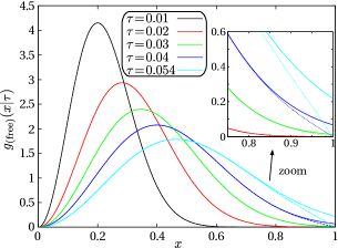
Figure 27: Illustration of the functions $g_{\text{free}}(x|\tau)$ and $g(x|\tau)$ for different times $t$. Full lines represent $g_{\text{free}}$, dotted ones $g$. For small $\tau$ the curves coincide almost perfectly.

As $g(x|\tau)\leq g_{\text{free}}(x|\tau)$ holds for all $x$ and $\tau$, the rejection sampling procedure for $\tilde{\rho}_{n}$ is the following:
We generate a random $x_{\text{c}}\in\;]0;1[$ according to $g_{\text{free}}(x|\tau)$ in a way, which will be described later. Afterwards it is accepted with probability $p_{a}=g(x_{\text{c}}|\tau)/g_{\text{free}}(x_{\text{c}}|\tau)$, which can be simplified to

$$p_{a}(x_{\text{c}}|\tau)=1+\frac{\sum\limits_{k=1}^{k_{\text{max}}(\tau)}\left((2k+x_{\text{c}})e^{\frac{-k(k+x_{\text{c}})}{\tau}}-(2k-x_{\text{c}})e^{\frac{-k(k-x_{\text{c}})}{\tau}}\right)}{x_{c}}\;.$$

Similar to the method in the previous subsection, it is possible to save a lot of computation time by having a closer look at the function $p_{a}(x_{\text{c}}|\tau)$ in order to formulate some preconditions for acceptance. For all $\tau\in[0;0.054]$ the following inequalities hold:

• $p_{a}(x_{\text{c}}|\tau)>0.98\;\forall x\in[0;0.75]$

• $p_{a}(x_{\text{c}}|\tau)>0.91\;\forall x\in[0.75;0.85]$

• $p_{a}(x_{\text{c}}|\tau)>0.55\;\forall x\in[0.85;0.95]$ ,

which is illustrated in Fig 28.

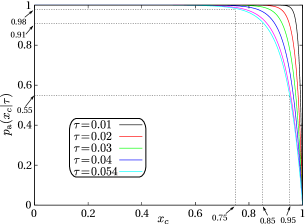
Figure 28: Illustration of the empirically chosen preconditions: For more than 95 $\%$ of the sampled $x_{c}$, the sampled rejection random number $r_{\text{rej}}$ will be within one of the three black dotted rectangles. There $x_{c}$ can be accepted without a calculation of $p_{a}(x_{\text{c}}|\tau)$.

Due to these chosen relations, in the worst case ($\tau=0.054$), for less than 5 $\%$ of the sampled $x_{c}$ it is necessary to calculate $p_{a}(x_{\text{c}}|\tau)$ for the decision whether to accept or to deny $x_{c}$.
Sampling the candidate $x_{c}$ is also done via rejection sampling: At first, we sample three gaussian random numbers $z_{1},\,z_{2},\,z_{3}$ with variance $\sigma^{2}=2\tau$ and calculate

$$x_{c}=\sqrt{z_{1}^{2}+z_{2}^{2}+z_{3}^{2}}\;.$$

For $x_{c}\leq 1$, which happens (again in the worst case) in more than 97 $\%$, we go on, otherwise we resample $x_{c}$ until it is smaller than 1.
A C++-implementation of the described method on a single CPU-core with 3.4 GHz takes for the worst case scenario ($\tau=0.054$) 160 sec for $10^{9}$ random $x$.

At first sight, this procedure consisting of two steps of rejection sampling might not look so fast, but apart from the very small rejection rates and its fast generation, there is a second argument, which speeds the procedure indirectly up: We don’t need to sample the solid angle for a position update any more, taking $z_{1},\,z_{2},\,z_{3}$ for the replacement fulfills the right statistics in this case.

A.4.2 Sampling for $\tau>0.054$

For very small values of $\tau$, the shape of $\tilde{\rho}_{n}$ changes very fast with time, which can also be seen in Fig. 27. But for $\tau\rightarrow\infty$ it converges quickly to the time independent density

$$\tilde{\rho}_{\infty}(x)=\pi x\sin{\pi x}\;.$$

Our sampling routine makes use of this fact by dividing the time interval $[0.054;\infty[$ into a sequence of $M$ disjoint intervals $[\tau_{j};\tau_{j+1}[$ with $\tau_{0}=0.054$ and $\tau_{M}=\infty$. Within every interval $[\tau_{i};\tau_{i+1}[$, we want to construct an efficient rejection sampling method with a time independent helping density $\rho_{j}(x)$ and a scaling constant $k_{j}$. In consequence, a lower boundary $B(\tau_{j},\tau_{j+1})$ for each scaling constant $k_{j}$ is given by

$$B(\tau_{j},\tau_{j+1})=\int_{0}^{1}dx\operatorname*{\text{max}}\limits_{\tau\in[\tau_{j};\tau_{j+1}]}(\tilde{\rho}_{n}(x,\tau))<k_{j}\;.$$

With the choice $M=9$ and the decomposition

$$I_{1}=[0.054;0.057[\,,\;I_{2}=[0.057;0.061[\,,\;I_{3}=[0.061;0.066[\;$$

$$I_{4}=[0.066;0.072[\;,\;I_{5}=[0.072;0.08[\;\;,\;\;I_{6}=[0.08;0.091[\;\;$$

$$I_{7}=[0.091;0.108[\;,\;I_{8}=[0.108;0.15[\;\;,\;\;I_{9}=[0.15;\infty[\;\;\;\;\;\;$$

we confirmed numerically

$$1.015<B(\tau_{j},\tau_{j+1})<1.028\quad\forall\;j\;.$$

Similar to the case of $\tilde{\rho}_{b}$, we divide the spatial interval $[0;1]$ $M$ times into $N_{j}$ intervals $[x_{i}^{j};x_{i+1}^{j}]$ with $x_{0}^{j}=0$ and $x_{N_{j}}^{j}=1$. For all $N_{j}$ intervals we want $\rho_{j}(x)$ to be piece-wise constant:

$$\rho_{j}(x)=\frac{p_{i}^{j}}{k_{j}}\quad\forall\;x\in[x_{i}^{j},x_{i+1}^{j}]\;,$$

with $p_{i}^{j}=\operatorname*{\text{max}}\limits_{\tau\in[\tau_{j};\tau_{j+1}]}\left(\operatorname*{\text{max}}\limits_{[x_{i}^{j},x_{i+1}^{j}]}\tilde{\rho}_{n}(x|\tau)\right)$. By choosing the length of the first intervals $[x_{0}^{j},x_{1}^{j}]\;\forall\;j$, we again define a set of constants $Q_{j}=(x_{1}-x_{0})\cdot p_{0}^{j}$ and the length of all the other intervals is determined via

$$(x_{i+1}^{j}-x_{i}^{j})\cdot p_{i}^{j}=Q_{j}\quad\;\forall\;i\in\left\{1..N_{j}-1\right\}\;.$$

In order to get $x_{i}^{j}$ and $p_{i}^{j}$ within double precision, its iteration was done with much more than double precision and took some minutes. But this also has to be done only once, when implementing the routine. The length of the last intervals is determined by $1-x_{N_{j}}$, in consequence, we get:

$$k_{j}=(N_{j}-1)\cdot Q_{j}+(1-x_{N_{j}})p_{N_{j}}\;.$$

Fig. 29 shows this decomposition for the case of $\tau\in I_{9}$ and the choice $x_{1}^{9}=0.08$.

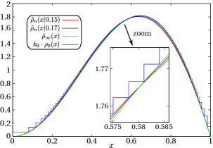
Figure 29: Illustration of the construction of $\rho_{9}(x)$ for the choice $x_{1}^{9}=0.08$, which results in N=194 intervals $[x_{i}^{9},x_{i+1}^{9}]$ and a scaling constant $k_{9}=1.02$.

In consequence, we get $N=194$ and $k_{9}=1.02...$, which results in a rejection rate of about $2\%$. Following the same argumentation as in the subsection before (same probability mass $1/N$ per interval), it is possible to generate random numbers according to all $\rho_{j}(x)$ very fast. Finally we go on as in all the other cases before: By having a closer look at the quotient $\tilde{\rho}_{n}/(k_{j}\rho_{j})$ once, we can avoid computing the time demanding computation of $\tilde{\rho}_{n}$ in more than $90\%$ of all cases by formulating some preconditions for accepting. A C++-implementation of the described method on a single CPU-core with 3.4 GHz takes around 65 sec for $10^{9}$ random $x$.

memory requirement

The last two subsections introduced very fast and exact recipes for sampling random numbers according to the densities $\rho_{b}(t)$ and $\rho_{n}(r|t)$. In most cases these recipes were based on the precalculation of fast invertable piece wise constant density functions for rejection sampling. The total memory requirement for these values is less than 36 kB.

References

- (1) J. Najemnik and W. S. Geisler, Journal of Vision 8, 1 (2008).
- (2) N. E. Humphries, N. Queiroz, J. R. M. Dyer, N. G. Pade, M. K. Musyl, K. M. Schaefer, D. W. Fuller, J. M. Brunnschweiler, et al., Nature 465, 1066 (2010).
- (3) N. R. Franks, T. O. Richardson, S. Keir, S. J. Inge, F. Bartumeus, and A. Sendova-Franks, Journal of Experimental Biology 213, 1697 (2010).
- (4) L. Li, S. F. Nørrelykke, and E. C. Cox, PLoS ONE 3, e2093 (2008).
- (5) S. Redner, A Guide to First-Passage Processes (University Press, Cambridge, 2001).
- (6) T. G. Mattos, C. Mejia-Monasterio, R. Metzler, and G. Oshanin, Phys. Rev. E 86, 031143 (2012).
- (7) H. Risken, The Fokker-Planck Equation: Methods of Solution and Applications (Springer, Berlin, 1996).
- (8) V. Tejedor, R. Voituriez, and O. Bénichou, Phys. Rev. Lett. 108, 088103 (2012).
- (9) O. Bénichou, D. Grebenkov, P. Levitz, C. Loverdo, and R. Voituriez, Phys. Rev. Lett. 105, 150606 (2010).
- (10) T. Calandre, O. Bénichou, and R. Voituriez, Phys. Rev. Lett. 112, 230601 (2014).
- (11) M. R. Evans and S. N. Majumdar, Phys. Rev. Lett. 106, 160601 (2011).
- (12) L. Kusmierz, S. N. Majumdar, S. Sabhapandit, and G. Schehr, Phys. Rev. Lett. 113, 220602 (2014).
- (13) O. Bénichou, M. Coppey, M. Moreau, PH Suet, and R. Voituriez, J. Phys. Condens. Matter 17, 4275 (2005).
- (14) O. Bénichou, M. Coppey, M. Moreau, PH Suet, and R. Voituriez, Phys. Rev. Lett. 94, 198101 (2005).
- (15) O. Bénichou, C. Loverdo, M. Moreau, and R. Voituriez, J. Phys. Condens. Matter 19, 065141 (2007).
- (16) P. Bressloff and J. Newby, New J. Phys 11, 023033 (2009).
- (17) O. Bénichou, C. Loverdo, M. Moreau, and R. Voituriez, Rev. Mod. Phys. 83, 81 (2011).
- (18) C. Loverdo, O. Benichou, M. Moreau, and R. Voituriez, Nat. Phys 4, 134 (2008).
- (19) C. Loverdo, O. Benichou, M. Moreau, and R. Voituriez, Phys. Rev. E 80, 031146 (2009).
- (20) D. A. Smith and R. M. Simmons, Biophys. J. 80, 45 (2001).
- (21) P. Bressloff and J. Newby, Phys. Rev. E 85, 031909 (2012).
- (22) B. Alberts et. al , Molecular Biology of the Cell, 6th ed. (Garland, New York, 2014).
- (23) K. Schwarz, Y. Schröder, B. Qu, M. Hoth and H. Rieger, Phys. Rev. Lett., in revision (2016); arXiv:160200509
- (24) P. L. Krapivsky and S. Redner, Am. J. Phys 64, 546 (1996).
- (25) O. Bénichou, M. Coppey, M. Moreau, PH Suet, and R. Voituriez, Europhys. Lett. 70, 42 (2005).
- (26) A. Singer, Z. Schuss, and D. Holcman, J. Stat. Phys. 122, 437 (2006).
- (27) A. Singer, Z. Schuss, and D. Holcman, J. Stat. Phys. 122, 465 (2006).
- (28) A. Singer, Z. Schuss, and D. Holcman, J. Stat. Phys. 122, 491 (2006).
- (29) A. Singer, Z. Schuss, and D. Holcman, Proc. Natl. Acad. Sci. USA 104, 16098 (2007).
- (30) Z. Schuss, J. Sci. Computing 53, 194 (2012)
- (31) O. Bénichou and R. Voituriez, Phys. Rev. Lett. 100, 168105 (2008).
- (32) C. Chevalier, O. Bénichou, and R. Voiturez, J. Phys. A 44, 025002 (2011).
- (33) A. F. Cheviakov, A. S. Reimer, and M. J. Ward, Phys. Rev. E 85, 021131 (2012).
- (34) P. L. Krapivsky and S. Redner J. Phys. A 29, 5347 (1996).
- (35) S. Redner and P. L. Krapivsky, Capture of the lamb: Diffusing predators seeking a diffusing prey, Am. J. Phys. 67, 1277 (1999).
- (36) J. S. van Zon and P. R. ten Wolde, Phys. Rev. Lett. 94, 128103 (2005).
- (37) J. S. van Zon and P. R. ten Wolde, J. Chem. Phys. 123, 234910 (2005).
- (38) T. Oppelstrup, V. V. Bulatov, G. H. Gilmer, M. H. Kalos, and B. Sadigh, Phys. Rev. Lett. 97, 230602 (2006).
- (39) T. Oppelstrup, V. V. Bulatov, A. Donev, M. H. Kalos, G. H. Gilmer, and B. Sadigh, Phys. Rev. E 80, 066701 (2009).
- (40) A. Donev, V. V. Bulatov, T. Oppelstrup, G. H. Gilmer, B. Sadigh, and M. H. Kalos, J. Comp. Phys. 229, 3214 (2010).
- (41) K. Schwarz and H. Rieger, J. Comp. Phys. 237, 396 (2013).
- (42) L. Devroye, Non-Uniform Random Variate Generation, (Springer, Heidelberg, 1986).
- (43) H. S. Carslaw and J. C. Jäger, Conduction of heat in solids, (University Press, Oxford, 1959).
- (44) M. Matsumoto and T. Nishimura, ACM Trans. Model. Comput. Simul. 8, 3 (1998).