Nonlinear light-Higgs coupling in superconductors beyond BCS:
Effects of the retarded phonon-mediated interaction

Abstract

We study the contribution of the Higgs amplitude mode on the nonlinear optical response of superconductors beyond the BCS approximation by taking into account the retardation effect in the phonon-mediated attractive interaction. To evaluate the vertex correction in nonlinear optical susceptibilities that contains the effect of collective modes, we propose an efficient scheme which we call the “dotted DMFT” based on the nonequilibrium dynamical mean-field theory (nonequilibrium DMFT) to go around the difficulty of solving the Bethe-Salpeter equation and analytical continuation. The vertex correction is represented by the derivative of the self-energy with respect to the external driving field, which is self-consistently determined by the differentiated (“dotted”) DMFT equations. We apply the method to the Holstein model, a prototypical electron-phonon-coupled system, to calculate the susceptibility for the third-harmonic generation including the vertex correction. The results show that, in sharp contrast to the BCS theory, the Higgs mode can contribute to the third-harmonic generation for general polarization of the laser field with an order of magnitude comparable to the contribution from the pair breaking or charge density fluctuations. The physical origin is traced back to the nonlinear resonant light-Higgs coupling, which has been absent in the BCS approximation.

I Introduction

Nonequilibrium dynamics of superconductors induced by intense laser excitations opens various possibilities of controlling emergent states of matter without destroying quantum coherence. Fausti et al. (2011); Cortés et al. (2011); Smallwood et al. (2012); Dal Conte et al. (2012); Kaiser et al. (2014); Matsunaga and Shimano (2012); Hinton et al. (2013); Man ; Matsunaga et al. (2013); Hu et al. (2014); Mankowsky et al. (2014); Mat ; Mitrano et al. (2016); Giannetti et al. (2016) Specifically, for relatively low frequencies of the laser such as terahertz (THz) and mid-infrared, we can expect to suppress the generation of quasiparticles having high energies that might be quickly transformed into heat through inelastic collisions causing a destruction of quantum coherence. Recent experiments indeed report that a superconducting-like state can be generated from the normal state by such low-energy excitations.Fausti et al. (2011); Kaiser et al. (2014); Hu et al. (2014); Mankowsky et al. (2014); Mitrano et al. (2016)

In superconductors, there exists a collective mode called the Higgs amplitude mode, which plays an important role in low-energy dynamics. The mode corresponds to the coherent amplitude oscillation of the superfluid density, which has a long history of theoretical studies. Anderson (1958); Nam ; Anderson (1963); Eng ; Hig ; Gur ; Vol (a); Lit ; Kul ; Varma (2002); Barankov et al. (2004); Yuzbashyan et al. (2006); Barankov and Levitov (2006); Yuzbashyan and Dzero (2006); Papenkort et al. (2007, 2008); Gurarie (2009); Schnyder et al. (2011); Podolsky et al. (2011); Vol (b); Tsuji et al. (2013); Barlas and Varma (2013); Tsuchiya et al. (2013); Gazit et al. (2013); Krull et al. (2014); Cea and Benfatto (2014); Pekker and Varma (2015); Kemper et al. (2015); Cea et al. (2015); Tsuji and Aoki (2015); Peronaci et al. (2015); Jujo (2015); Kru ; Murakami et al. (2016); Cea et al. (2016); Mur (a, b) Experimental observation of the Higgs mode in superconductors has been reported by Raman scattering, Sooryakumar and Klein (1980); Méasson et al. (2014) and THz pump-probe experiments.Matsunaga et al. (2013); Mat It has also been reported in a THz pump experimentMat that there emerges a third-harmonic generation (THG) in the nonlinear optical response that is resonantly enhanced when the doubled frequency ($2\Omega$) of the incident light equals the superconducting gap ($2\Delta$), which coincides with the energy of the collective Higgs mode at long wavelength. On the other hand, there also exist individual excitations (Cooper pair breaking or charge density fluctuations), whose lower bound in the energy spectrum resides at the same energy of $2\Delta$ with a diverging density of states. The question then is to what extent these two contribute to the nonlinear optical response in superconductors and how strongly the light is nonlinearly coupled to the Higgs mode.Tsuji and Aoki (2015); Cea et al. (2016)

In the BCS mean-field theory (with the random phase approximation), the contribution of pair breaking or charge density fluctuation to the THG susceptibility is expressed in a gauge invariant form (including the screening effect) asCea et al. (2016)

$$\chi_{0}^{\rm BCS}(\Omega) =\sum_{\bm{k}}(\ddot{\epsilon}_{\bm{k}})^{2}\chi_{33}(\bm{k},\Omega)-\frac{\left[\sum_{\bm{k}}\ddot{\epsilon}_{\bm{k}}\chi_{\rm 33}(\bm{k},\Omega)\right]^{2}}{\sum_{\bm{k}}\chi_{\rm 33}(\bm{k},\Omega)}.$$ (1)

Here $\epsilon_{\bm{k}}$ is the band dispersion, $\ddot{\epsilon}_{\bm{k}}=\sum_{ij}(\partial^{2}\epsilon_{\bm{k}}/\partial k_{i}\partial k_{j})e_{i}e_{j}$, $\bm{e}$ is the polarization vector of light, and

$$\chi_{33}(\bm{k},\Omega) =-\frac{i}{2}\int\frac{d\omega}{2\pi}{\rm Tr}[\tau_{3}\hat{G}_{\bm{k}}(\omega+2\Omega)\tau_{3}\hat{G}_{\bm{k}}(\omega)]^{<},$$ (2)

where $\tau_{3}$ is the third component of the Pauli matrix, $\hat{G}_{\bm{k}}(\omega)$ is the Nambu-Gor’kov Green’s function, and $<$ denotes the lesser component based on the Langreth ruleLan (with the notation defined in Appendix A). For $s$-wave superconductors, $\hat{G}_{\bm{k}}(\omega)$ and $\chi_{33}(\bm{k},\omega)$ depend respectively on the momentum through $\epsilon_{\bm{k}}$, which allows one to change the momentum sum into an energy integral by inserting $1=\int d\epsilon\delta(\epsilon-\epsilon_{\bm{k}})$. Then we can define expansions around the Fermi energy,Tsuji and Aoki (2015); Mur (a)

$$\sum_{\bm{k}}\delta(\epsilon-\epsilon_{\bm{k}})\ddot{\epsilon}_{\bm{k}} =D(\epsilon_{F})(c_{0}+c_{1}\epsilon+c_{2}\epsilon^{2}+\cdots),$$ (3)

$$\sum_{\bm{k}}\delta(\epsilon-\epsilon_{\bm{k}})(\ddot{\epsilon}_{\bm{k}})^{2} =D(\epsilon_{F})(\tilde{c}_{0}+\tilde{c}_{1}\epsilon+\tilde{c}_{2}\epsilon^{2}+\cdots),$$ (4)

where $D(\epsilon_{F})$ is the density of states at the Fermi energy. In Ref. Tsuji and Aoki, 2015, it is assumed that the constant terms in the expansions (3) and (4) can be removed by gauge transformations, so that the pair breaking effect in THG is less dominant than the Higgs mode. As pointed out in Ref. Cea et al., 2016, however, this holds in rather restricted situations, such as one dimensional (1D) lattices, 2D square and 3D simple cubic lattices with polarization $\bm{e}$ respectively parallel to $(1,1)$ and $(1,1,1)$ directions, 3D body-centered-cubic lattice with $\bm{e}$ parallel to $(1,0,0)$, and so on. For a general lattice with a general polarization, the constant terms may survive, and the Higgs-mode contribution may be left subleading.

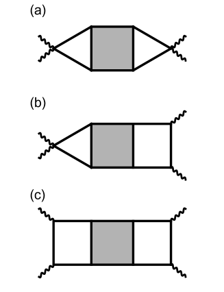
Figure 1: Feyman diagrams for the non-resonant (a), mixed (b), and resonant (c) contributions to the THG susceptibility containing the effect of collective modes as vertex corrections. The solid (wavy) lines represent the electron (photon) propagators, while the shaded boxes represent the reducible four-point vertex function. Among the four photon lines, one is outgoing with an energy $3\Omega$, and the other three are incoming with an energy $\Omega$.

Then the next question is: what will happen if one goes beyond the BCS approximation. In fact, the superconductor NbN used in the experimentsMatsunaga et al. (2013); Mat is known to have a strong electron-phonon coupling ($\lambda\sim 1$), Kihlstrom et al. (1985); Brorson et al. (1990); Chockalingam et al. (2008) where it is important to capture corrections from the BCS analysis. Indeed the argument in the previous paragraph heavily relies on the speciality of BCS: the (nonlinear) coupling to the light occurs only in a non-resonant form $\ddot{\epsilon}_{\bm{k}}A(t)^{2}$ rather than in a resonant form $\dot{\epsilon}_{\bm{k}}A(t)\dot{\epsilon}_{\bm{k}}A(t^{\prime})$, where $\bm{A}(t)=A(t)\bm{e}$ is the vector potential, and $\dot{\epsilon}_{\bm{k}}=\sum_{i}(\partial\epsilon_{\bm{k}}/\partial k_{i})e_{i}$. The terminology (“resonant” and “non-resonant”) is here borrowed from literatures on Raman scattering.Devereaux and Hackl (2007) These forms can be expressed as diagrams for the THG susceptibility Butcher and Cotter (1998) in Fig. 1 (which in fact very much resemble Raman-scattering diagramsDevereaux and Hackl (2007)), where the effect of collective modes is incorporated in the vertex correction, with the Higgs mode represented by an infinite series of ring diagrams in the $\tau_{1}$ channel.Lit ; Varma (2002); Pekker and Varma (2015); Tsuji and Aoki (2015) Two photon lines attached together to electron lines represent the non-resonant coupling, while two single-photon lines attached separately represent the resonant coupling.

Within the BCS theory, there is only the non-resonant coupling, and the mixed [Fig. 1(b)] and resonant (c) contributions to THG exactly vanish. This is confirmed by explicitly calculating the convolution of relevant three electron propagators,

$$\int\frac{d\omega}{2\pi}{\rm Tr}[\tau_{1}\hat{G}_{\bm{k}}(\omega+2\Omega)\hat{G}_{\bm{k}}(\omega+\Omega)\hat{G}_{\bm{k}}(\omega)]^{<} =0\quad(\mbox{BCS}).$$ (5)

However, this does not guarantee that these contributions would remain small if one goes beyond the BCS approximation. For example, the real part of the optical conductivity $\sigma(\Omega)$ vanishes for $\Omega\neq 0$ within the BCS theory, since

$$\int\frac{d\omega}{2\pi}{\rm Tr}[\hat{G}_{\bm{k}}(\omega+\Omega)\hat{G}_{\bm{k}}(\omega)]^{<} =0\quad(\mbox{BCS}),$$ (6)

in much the same way as in Eq. (5). In reality, however, the real part of the optical conductivity is nonzero and not even small.Matsunaga et al. (2013); Zimmermann et al. (1991) They become nonzero when one takes account of dynamical correlations such as the electron-phonon coupling (producing retarded interactions) or impurity scattering. In those situations, we can expect that the resonant and mixed contributions to the THG response may also be nonzero. Indeed, it has been shown in the study of Raman scattering for correlated electron systems that the resonant contribution can significantly enhance the non-resonant Raman response.Shvaika et al. (2004, 2005)

This has motivated us to study here the nonlinear optical response of superconductors for electron-phonon coupled systems beyond the BCS approximation. Theoretically, it is quite challenging to evaluate all of the non-resonant, mixed and resonant diagrams involving the four-point vertex on an equal footing, since the vertex carries three independent momenta and frequencies. Therefore, we employ the dynamical mean-field theory (DMFT),Georges et al. (1996) which assumes the momentum-independent self-energy and vertex function. Still, the calculation is quite demanding if one tries to evaluate the nonlinear response function by solving the Bethe-Salpeter equation and performing multiple analytical continuations. In higher dimensions in the thermodynamic limit, an analysis including the vertex correction has so far been performed only in exceptional cases, such as the Raman response of the Falicov-Kimball model. Shvaika et al. (2004, 2005); Freericks and Zlatić (2003); Matveev et al. (2010) For the Hubbard model, the nonlinear optical response has been analyzed by Hartree-Fock approximation,Jujo (2006) by DMFT without considering vertex corrections,Jujo (2008, 2009) and by exact diagonalization for small finite-size systems.Mizuno et al. (2000); Takahashi et al. (2002) For the Holstein model, higher-harmonic generation has been studied by Migdal approximation without considering vertex corrections.Kemper et al. (2013) For 1D Hubbard-Holstein model, THG response has been studied by the density-matrix renormalization group.Sota et al. (2015)

In this paper, we propose an efficient way to calculate the vertex correction for nonlinear optical susceptibilities, which we call the “dotted DMFT”Tsu , without directly solving the Bethe-Salpeter equation and performing analytical continuation. The idea is to let the nonequilibrium DMFT equationsAoki et al. (2014) differentiated (“dotted”) with respect to the external field to deduce a self-consistent equation for the vertex function represented by the dotted self-energy. We then apply the method to the Holstein model, a prototypical model for electrons interacting with local phonons giving retarded interactions among electrons. The results indicate that the resonant contribution from the Higgs mode to the THG susceptibility can indeed be comparable to those from the pair breaking or density fluctuations. In particular, the resonance of THG at $2\Omega=2\Delta$ can be enhanced by the nonlinear resonant coupling between the light and Higgs mode.

The paper is organized as follows. In Sec. II, we describe the model set-up that we use throughout the paper for the analysis of the nonlinear optical response in superconductors. In Sec. III, we propose an efficient method (dotted DMFT) to evaluate the vertex correction for dynamical susceptibilities based on the nonequilibrium DMFT. Sec. IV describes the results of the THG susceptibility obtained by the dotted DMFT for the electron-phonon-coupled system. In Sec. V we summarize the paper.

II Model

We take the Holstein model as a typical model for electrons interacting with local phonons,

$$H =\sum_{ij,\sigma}t_{ij}(c_{i\sigma}^{\dagger}c_{j\sigma}+{\rm h.c.})-\mu\sum_{i}n_{i}$$

$$\quad+\omega_{0}\sum_{i}b_{i}^{\dagger}b_{i}+g\sum_{i}(b_{i}+b_{i}^{\dagger})(n_{i}-1).$$ (7)

Here $c_{i\sigma}^{\dagger}$ ($c_{i\sigma}$) is the creation (annihilation) operator for an electron at site $i$ with spin $\sigma=\uparrow,\downarrow$, $t_{ij}$ is the hopping amplitude, $n_{i}=\sum_{\sigma}c_{i\sigma}^{\dagger}c_{i\sigma}$, $\mu$ is the chemical potential, $b_{i}^{\dagger}$ ($b_{i}$) is the creation (annihilation) operator for phonons having a frequency $\omega_{0}$, and $g$ is the electron-phonon coupling constant. We then apply the dynamical mean-field theory (DMFT) to solve the model. Since DMFT becomes exact for large spatial dimensions ($d\to\infty$), Metzner and Vollhardt (1989); Georges et al. (1996) we take the hypercubic lattice, whose energy dispersion is

$$\epsilon_{\bm{k}} =-2t\sum_{i=1}^{d}\cos k_{i}.$$ (8)

As usually done, we scale the hopping as $t=t^{\ast}/\sqrt{2d}$ with a fixed $t^{\ast}$ to obtain a meaningful fixed point in the large $d$ limit, which results in a gaussian density of states $D(\epsilon)=e^{-\epsilon^{2}/2t^{\ast}{}^{2}}/\sqrt{2\pi}t^{\ast}$. We use $t^{\ast}$ as the unit of energy (frequency) throughout the paper. We concentrate on the half-filled electron system ($\mu=0$), in which the particle-hole symmetry is fully respected. In the particle-hole symmetric case, the Higgs amplitude mode is safely decoupled from the phase mode, and the screening effect is absent. Away from half filling, the amplitude mode can hybridize with the phase mode in principle. However, we expect that the damping of the amplitude mode into the phase mode is suppressed in superconductors, since the phase mode is pushed to high energies ($\sim$ the plasma frequency) due to the Anderson-Higgs mechanism.Anderson (1963); Eng ; Hig ; Gur

If one integrates out the phonon degrees of freedom, the electrons acquire an effective retarded interaction,

$$U(\omega) =g^{2}D_{0}^{R}(\omega),$$ (9)

where $D_{0}^{R}(\omega)$ is the noninteracting retarded phonon Green’s function,

$$D_{0}^{R}(\omega) =\frac{2\omega_{0}}{(\omega+i\gamma)^{2}-\omega_{0}^{2}}.$$ (10)

We introduce a parameter $\gamma$ to regularize the phonon Green’s function. In the static limit ($\omega\to 0$), the effective interaction approaches $U(\omega=0)=-2g^{2}\omega_{0}/(\omega_{0}^{2}+\gamma^{2})<0$, i.e., the attractive interaction. The strength of the attractive interaction can be measured (within the unrenormalized Migdal approximation as introduced later) by a dimensionless parameter,

$$\lambda \equiv|U(\omega=0)|D(\epsilon_{F})=\frac{2g^{2}\omega_{0}}{\omega_{0}^{2}+\gamma^{2}}D(\epsilon_{F}).$$ (11)

When the attractive interaction is large enough and the temperature is low enough, the model exhibits a phase transition from the normal to superconducting states.

In this paper, instead of taking the infinitesimal limit of $\gamma$ ($\to+0$), we keep it nonzero and regard it as a phenomenological parameter that represents the finite lifetime ($\tau\sim\gamma^{-1}$) of phonon oscillations. This is physically natural, since the phonon oscillation should be damped to some extent in real solids by various possible ways of scattering and energy dissipation. The electron-phonon coupling itself can induce the damping of phonons.Murakami et al. (2015) A finite $\gamma$ is not necessarily phenomenological, but can be actually modeled by phonons coupled to a heat bath comprising many harmonic oscillators (Caldeira-Leggett-type modelCaldeira and Leggett (1983)). In the application of the dotted DMFT, which we shall introduce in the next section, it turns out that it is important to take a nonzero $\gamma$ (avoiding infinitely long-lived phonons) to stabilize the convergence of the dotted DMFT calculation.

In a similar manner, we introduce a small imaginary part $\delta$ (broadening factor) in the noninteracting retarded electron Green’s function,

$$G_{0\bm{k}}^{R}(\omega) =\frac{1}{\omega+i\delta+\mu-\epsilon_{\bm{k}}},$$ (12)

where $\delta$ can be considered as a decay rate of noninteracting electrons. It can be modeled by electrons coupled to a bath composed of free fermions.Aoki et al. (2014); Tsuji et al. (2009) Compared to $\gamma$, the stability of the dotted DMFT is less sensitive to $\delta$, so that we can take a much smaller value for $\delta$ than for $\gamma$.

To study the third-harmonic generation, we apply an ac electric field to the Holstein model. We use the temporal gauge to represent the electric field with a vector potential $\bm{A}(t)=\bm{e}Ae^{-i\Omega t}$, where $\bm{e}$ is the polarization vector ($||\bm{e}||=1$), $A$ and $\Omega$ is the amplitude and frequency of the vector potential, respectively. $A$ is related to the amplitude of the electric field $E$ via $A=E/(i\Omega)$. The ac field is minimally coupled to the electrons through the Peierls phase. The resulting form of the coupling is $\sum_{\bm{k}\sigma}\epsilon_{\bm{k}+\bm{A}(t)}c_{\bm{k}\sigma}^{\dagger}c_{\bm{k}\sigma}$ in the kinetic term of the Hamiltonian, where we have put the elementary charge $e=1$. The electron current is defined by

$$\bm{j}(t) =-i\sum_{\bm{k}}\bm{v}_{\bm{k}+\bm{A}(t)}G_{\bm{k}}^{<}(t,t),$$ (13)

where $\bm{v}_{\bm{k}}=\partial\epsilon_{\bm{k}}/\partial{\bm{k}}$ is the group velocity. We measure the current along the electric field,

$$j(t)=\bm{j}(t)\cdot\bm{e}.$$ (14)

The susceptibility for the third-harmonic generation $\chi(\Omega)$ is defined by the nonlinear current oscillating with the frequency $3\Omega$,

$$j^{(3)}(t) =\chi(\Omega)A^{3}e^{-3i\Omega t}.$$ (15)

To obtain the THG susceptibility, we take the third derivative of Eq. (13) with respect to $A$ and then set $A=0$. This involves the derivatives of $G$, which are evaluated by means of the dotted DMFT, as will be explained in the next section.

Since our model is infinite dimensional, it is not obvious how to choose the polarization. One convenient way is to take the direction parallel to $(1,1,\dots,1)$, for which every direction is equivalent. However, as mentioned in the introduction, this choice has a bias that the pair breaking effect is suppressed in the THG response. Another simple choice is $(1,0,\dots,0)$. This, on the other hand, is the direction that maximally enhances the pair breaking contribution. To let the situation as fair as possible, we choose a general direction

$$\bm{e}\propto(\overbrace{\underbrace{1,1,\dots,1}_{m},0,\dots,0}^{d}),$$ (16)

where $m$ is the number of dimensions along which the polarization vector has nonzero components. It is a kind of generalization of $(1,1,0)$ direction for the three-dimensional cubic lattice. We fix the ratio,

$$\alpha=\frac{m}{d}\quad(0\leq\alpha\leq 1),$$ (17)

and take the limit of $d,m\to\infty$. The parameter $\alpha$ continuously interpolates the two limits of $(1,1,\dots,1)$ and $(1,0,\dots,0)$.

The advantage of this setup is that it greatly simplifies the momentum integral without putting a bias on the pair breaking effect. We need a very fine grid for the momentum integral to eliminate the finite-size effect, which is particularly severe in the calculation of the THG spectrum, since one has to resolve the superconducting gap structure in the very vicinity of the Fermi energy. One might apply DMFT to the two-dimensional square lattice as an approximation (instead of applying to the hypercubic lattice), but our experience indicates that the number of $k$ points that has to be taken is so huge that it is practically intractable.

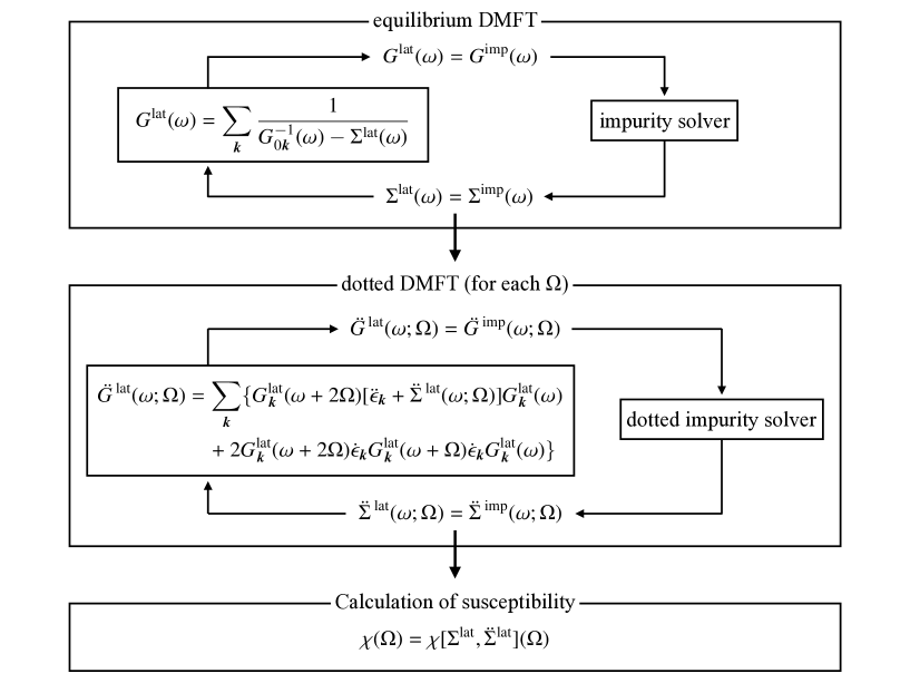
Figure 2: A schematic picture for the dotted dynamical mean-field theory (dotted DMFT) formalism for the third-harmonic generation. Each equation holds for the retarded, advanced, lesser, and greater Green’s functions and self-energies, respectively. An analogous treatment can be generally applied to arbitrary dynamical susceptibilities.

To see how the momentum integral is simplified, we expand $\epsilon_{\bm{k}+\bm{A}(t)}$ in $A$ as

$$\epsilon_{\bm{k}+\bm{A}(t)} =\epsilon_{\bm{k}}+\dot{\epsilon}_{\bm{k}}Ae^{-i\Omega t}+\frac{1}{2}\ddot{\epsilon}_{\bm{k}}A^{2}e^{-2i\Omega t}+\cdots,$$ (18)

where the dot denotes the derivative with respect to $A$, that is,

$$\dot{\epsilon}_{\bm{k}} =\sum_{i=1}^{d}\frac{\partial\epsilon_{\bm{k}}}{\partial k_{i}}e_{i},$$ (19)

$$\ddot{\epsilon}_{\bm{k}} =\sum_{i,j=1}^{d}\frac{\partial^{2}\epsilon_{\bm{k}}}{\partial k_{i}\partial k_{j}}e_{i}e_{j},$$ (20)

and so on. The THG susceptibility is expressed as a momentum integral of a function of $\epsilon_{\bm{k}}$ multiplied by some of $\dot{\epsilon}_{\bm{k}},\ddot{\epsilon}_{\bm{k}},\dddot{\epsilon}_{\bm{k}}$, and $\ddddot{\epsilon}_{\bm{k}}$ [with the total number of derivatives being always four since $\bm{v}_{\bm{k}}$ in the definition of the current (13) contains one derivative while the other three come from the external field]. For instance, let us consider a momentum integral of the form

$$\quad\sum_{\bm{k}}\dot{\epsilon}_{\bm{k}}\dddot{\epsilon}_{\bm{k}}f(\epsilon_{\bm{k}})$$

$$=\frac{1}{m^{2}}\sum_{\bm{k}}\sum_{i=1}^{m}2t\sin k_{i}\sum_{j=1}^{m}(-2t)\sin k_{j}f(\epsilon_{\bm{k}})$$

$$=-\frac{4t^{2}}{m^{2}}\sum_{\bm{k}}\left(\sum_{i=1}^{m}\sin^{2}k_{i}+\sum_{\begin{subarray}{c}i,j=1\\ i\neq j\end{subarray}}^{m}\sin k_{i}\sin k_{j}\right)f(\epsilon_{\bm{k}})$$ (21)

with a certain function $f(\epsilon)$. Since directions $i=1,\dots,m$ are equivalent and the second term in the parentheses vanishes due to a cancellation between $k_{i}$ and $-k_{i}$, we can simplify Eq. (21) as

$$=-\frac{4t^{2}}{m^{2}}\sum_{\bm{k}}m\sin^{2}k_{x}f(\epsilon_{\bm{k}}).$$ (22)

We can symmetrize the momenta $\{k_{i}\}$ in the integrand due to the cubic symmetry to have

$$=-\frac{4t^{2}}{m^{2}}\sum_{\bm{k}}\frac{m}{d}\sum_{i=1}^{d}\sin^{2}k_{i}f(\epsilon_{\bm{k}})$$

$$=-\frac{4t^{2}}{m^{2}}\sum_{\bm{k}}\frac{m}{d}\left(\sum_{i=1}^{d}\sin k_{i}\right)^{2}f(\epsilon_{\bm{k}}),$$ (23)

where $4t^{2}(\sum_{i=1}^{d}\sin k_{i})^{2}$ can be replaced by $t^{\ast}{}^{2}$ using the joint density of statesTurkowski and Freericks (2005) $D(\epsilon,\bar{\epsilon})=D(\epsilon)D(\bar{\epsilon})$ (with $\bar{\epsilon}=2t\sum_{i}\sin k_{i}$) and $\int d\bar{\epsilon}D(\bar{\epsilon})\bar{\epsilon}^{2}=t^{\ast}{}^{2}$. Equation (21) is finally reduced to

$$\sum_{\bm{k}}\dot{\epsilon}_{\bm{k}}\dddot{\epsilon}_{\bm{k}}f(\epsilon_{\bm{k}})=-\frac{t^{\ast}{}^{2}}{d^{2}\alpha}\sum_{\bm{k}}f(\epsilon_{\bm{k}})$$ (24)

in the infinite-dimensional limit. The resulting form can be expressed as a single integral of a function of $\epsilon=\epsilon_{\bm{k}}$, which can be evaluated analytically in terms of the local Green’s function and self-energy. Similar simplifications apply to all the possible terms in the THG susceptibility. In Appendix B we summarize some useful formulae to simplify various types of momentum integrals.

III Dotted DMFT

In this section, we propose an efficient way to calculate the vertex correction for nonlinear dynamical susceptibilities, which we call the “dotted DMFT” (Fig. 2). This is because the method enables us to evaluate derivatives of Green’s function and the self-energy with respect to the external field, which are required to obtain nonlinear response functions. We explain the formulation in the context of third-harmonic generation here, but it can be generalized to arbitrary dynamical susceptibilities.

To start with, let us assume that the system reaches the (time-periodic) nonequilibrium steady state in the long-time limit in the presence of an ac electric field. The steady state emerges due to the balance between continuous excitations by the electric field and an energy dissipation to a heat bath, i.e., the system considered must be an open system.

In the time-periodic nonequilibrium steady state, the time translational symmetry is partially recovered for Green’s function, $G(t+\mathcal{T},t^{\prime}+\mathcal{T})=G(t,t^{\prime})$ (with $\mathcal{T}=2\pi/\Omega$ being the period of the driving field). In principle, one can determine the interacting Green’s function within the nonequilibrium steady-state DMFT, or Floquet DMFT, Aoki et al. (2014); Tsuji et al. (2008) which is capable of treating an arbitrarily large amplitude of the electric field. For the present purpose, on the other hand, it is sufficient to calculate Green’s function up to the third order in the driving field.

This motivates us to expand Green’s function and the self-energy with respect to the driving field,

$$G(t,t^{\prime}) =G_{\rm eq}(t,t^{\prime})+\dot{G}(t,t^{\prime};\Omega)Ae^{-i\Omega t^{\prime}}$$

$$\quad+\frac{1}{2}\ddot{G}(t,t^{\prime};\Omega)A^{2}e^{-2i\Omega t^{\prime}}+\cdots,$$ (25)

$$\Sigma(t,t^{\prime}) =\Sigma_{\rm eq}(t,t^{\prime})+\dot{\Sigma}(t,t^{\prime};\Omega)Ae^{-i\Omega t^{\prime}}$$

$$\quad+\frac{1}{2}\ddot{\Sigma}(t,t^{\prime};\Omega)A^{2}e^{-2i\Omega t^{\prime}}+\cdots.$$ (26)

Here $G_{\rm eq}(t,t^{\prime})$ and $\Sigma_{\rm eq}(t,t^{\prime})$ are the equilibrium Green’s function and self-energy, respectively, and the external field is assumed to be in a form of $\bm{A}(t)={\bm{e}}Ae^{-i\Omega t}$. If one considers a real field such as $\bm{A}(t)={\bm{e}}A\cos\Omega t$, one has to extend the expansion including cross terms between $e^{-i\Omega t}$ and $e^{i\Omega t}$. There is an ambiguity in the definition of the expansion coefficients: the factor $e^{-in\Omega t^{\prime}}$ in the $n$th order can be replaced by $e^{-in\Omega[xt+(1-x)t^{\prime}]}$ ($x\in\mathbb{R}$). This is possible as long as the condition $G(t+\mathcal{T},t^{\prime}+\mathcal{T})=G(t,t^{\prime})$ holds. In this paper, we adopt the convention with $x=0$.

The advantage of expanding Green’s function with respect to $A$ rather than directly treating the nonequilibrium Green’s function is that the full time-translation symmetry is available at each order in the expansion. To see this, let us write the expansion as

$$G(t,t^{\prime}) =G_{\rm eq}(t,t^{\prime})+G^{(1)}(t,t^{\prime};\Omega)A+\frac{1}{2}G^{(2)}(t,t^{\prime};\Omega)A^{2}+\cdots.$$ (27)

At the $n$th order, the term contains multiple of $n$ ac fields, so that it acquires the phase $e^{-in\Omega\bar{t}}$ when time translation $t\to t+\bar{t}$ is operated. For example, for $n=2$ we have

$$G^{(2)}(t+\bar{t},t^{\prime}+\bar{t};\Omega) =e^{-2i\Omega\bar{t}}G^{(2)}(t,t^{\prime};\Omega).$$ (28)

Since $G^{(2)}(t,t^{\prime})=\ddot{G}(t,t^{\prime})e^{-2i\Omega t^{\prime}}$ by definition, $\ddot{G}$ becomes time-translation invariant:

$$\ddot{G}(t+\bar{t},t^{\prime}+\bar{t};\Omega) =\ddot{G}(t,t^{\prime};\Omega).$$ (29)

The same applies to all orders. This allows us to write $\ddot{G}(t,t^{\prime};\Omega)$ as a single-time function $\ddot{G}(t-t^{\prime};\Omega)\equiv\ddot{G}(t,t^{\prime};\Omega)$, which can be Fourier transformed as

$$\ddot{G}(t-t^{\prime};\Omega) =\int\frac{d\omega}{2\pi}e^{-i\omega(t-t^{\prime})}\ddot{G}(\omega;\Omega).$$ (30)

This is a great advantage because it is no longer necessary to treat the two-time Green’s function $G(t,t^{\prime})$ in favor of a single-frequency function. The following formulation can be implemented in the same way as in equilibrium which enjoys the full time-translation symmetry.

Now the task is to evaluate the expansion coefficients order by order. When the system has an inversion symmetry, the local Green’s function and self-energy must be parity even, while the electric field is parity odd. This implies that odd-order expansion coefficients identically vanish. The leading contribution then comes from the second order.

In order to determine the expansion coefficients, we differentiate every DMFT self-consistency equation with respect to $A$, and extract the second-order coefficients. Let us start with the lattice Dyson equation, $G=\sum_{\bm{k}}(G_{0\bm{k}}^{-1}-\Sigma)^{-1}$. If we take a double derivative with respect to $A$ on both sides of the equation (and use $\dot{\Sigma}=0$), we end up with the “dotted lattice Dyson equation”,

$$\ddot{G}^{R,A,<,>}(\omega;\Omega)=\sum_{\bm{k}}\big{\{}G_{\bm{k}}(\omega+2\Omega)[\ddot{\epsilon}_{\bm{k}}+\ddot{\Sigma}(\omega;\Omega)]G_{\bm{k}}(\omega)$$

$$\quad+2G_{\bm{k}}(\omega+2\Omega)\dot{\epsilon}_{\bm{k}}G_{\bm{k}}(\omega+\Omega)\dot{\epsilon}_{\bm{k}}G_{\bm{k}}(\omega)\big{\}}^{R,A,<,>},$$ (31)

where $R,A,<$, and $>$ denote the retarded, advanced, lesser, and greater components of nonequilibrium Green’s functions, respectively. For the detailed definition we refer to Ref. Aoki et al., 2014. For the notation of $R,A,<$, and $>$ for products of nonequilibrium Green’s functions, see Appendix A. Note that when Green’s function has a matrix form (as in the superconducting state), $\ddot{\hat{G}}^{A}(\omega;\Omega)\neq[\ddot{\hat{G}}^{R}(\omega;\Omega)]^{\dagger}$, so that the advanced component has to be calculated independently of the retarded one.

Similarly, we differentiate the impurity Dyson equation, $G=(\mathcal{G}_{0}^{-1}-\Sigma)^{-1}$ (with $\mathcal{G}_{0}$ being the Weiss Green’s function) twice with respect to $A$ to obtain the “dotted impurity Dyson equation”,

$$\ddot{G}^{R,A,<,>}(\omega;\Omega) =-\{G(\omega+2\Omega)[(\ddot{\mathcal{G}}_{0}^{-1})(\omega;\Omega)$$

$$\quad-\ddot{\Sigma}(\omega;\Omega)]G(\omega)\}^{R,A,<,>}.$$ (32)

Here the double-dotted inverse of the Weiss Green’s functions reads

$$(\ddot{\mathcal{G}}_{0}^{-1})^{R,A,<,>}(\omega;\Omega) =-[\mathcal{G}_{0}^{-1}(\omega+2\Omega)\ddot{\mathcal{G}}_{0}(\omega;\Omega)\mathcal{G}_{0}^{-1}(\omega)]^{R,A,<,>}.$$ (33)

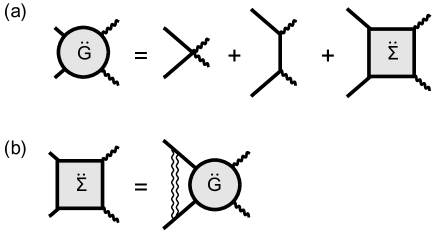
Figure 3: Diagrammatic representations of the dotted lattice Dyson equation (31) (a), and the dotted Migdal approximation (35) (b). The solid, wavy, and double-wavy lines represent the electron, photon, and phonon propagators, respectively.

To close the equation for the dotted functions, we need an explicit (diagrammatic) solution for the nonequilibrium impurity problem. This depends on the model and approximation. In the present case of the Holstein model, we employ the (unrenormalized) Migdal approximation,Kemper et al. (2015); Sen ; Murakami et al. (2016); Mur (b)

$$\Sigma^{<,>}(t,t^{\prime}) =ig^{2}D_{0}^{<,>}(t,t^{\prime})G^{<,>}(t,t^{\prime}),$$ (34)

which assumes that phonons stay in equilibrium. After expanding $\Sigma$ and $G$ with respect to $A$ as in Eqs. (25) and (26), and compare both sides of the equation at the order $A^{2}$, we obtain

$$\ddot{\Sigma}^{<,>}(t;\Omega) =ig^{2}D_{0}^{<,>}(t)\ddot{G}^{<,>}(t;\Omega).$$ (35)

The corresponding retarded and advanced components are given by

$$\ddot{\Sigma}^{R}(t;\Omega) =\theta(t)[\ddot{\Sigma}^{>}(t;\Omega)-\ddot{\Sigma}^{<}(t;\Omega)],$$ (36)

$$\ddot{\Sigma}^{A}(t;\Omega) =\theta(-t)[\ddot{\Sigma}^{<}(t;\Omega)-\ddot{\Sigma}^{>}(t;\Omega)],$$ (37)

where $\theta(t)=1$ for $t\geq 0$ and $=0$ otherwise (step function). In this way, the dotted DMFT naturally generates the impurity solver that is consistent with the approximation used in the equilibrium DMFT. The diagrammatic representation of the dotted lattice Dyson equation (31) and dotted Migdal approximation (35) are shown in Fig. 3. In particular, if we expand the dotted self-energy only with $G$ and $D_{0}$, it has a ladder structure, which represents the contribution from the amplitude mode.Murakami et al. (2016)

The technique can be applied to any models in principle, as far as the diagrammatic expression for the impurity problem is given. To see how it works further, let us take another prototypical example, the Hubbard model,

$$H =\sum_{ij}t_{ij}c_{i\sigma}^{\dagger}c_{j\sigma}+U\sum_{i}n_{i\uparrow}n_{i\downarrow},$$ (38)

where $U$ is the on-site Coulomb interaction. The Hubbard model is of particular interest in its own right from the point of view of large nonlinear optical responses of Mott insulators.Kishida et al. (2000, 2001) The diagrammatic approximation often used for the nonequilibrium impurity problem is the iterative perturbation theory (IPT),Georges and Kotliar (1992); Georges et al. (1996)

$$\Sigma_{\sigma}^{<,>}(t,t^{\prime}) =U^{2}\mathcal{G}_{0,\sigma}^{<,>}(t,t^{\prime})\mathcal{G}_{0,-\sigma}^{>,<}(t^{\prime},t)\mathcal{G}_{0,-\sigma}^{<,>}(t,t^{\prime}),$$ (39)

which is nothing but the bare second-order weak-coupling perturbation theory. The dotted impurity solution derived from IPT is given as

$$\ddot{\Sigma}_{\sigma}^{<,>}(t;\Omega) =U^{2}\ddot{\mathcal{G}}_{0,\sigma}^{<,>}(t;\Omega)\mathcal{G}_{0,-\sigma}^{>,<}(-t)\mathcal{G}_{0,-\sigma}^{<,>}(t)$$

$$\quad+U^{2}e^{-2i\Omega t}\mathcal{G}_{0,\sigma}^{<,>}(t)\ddot{\mathcal{G}}_{0,-\sigma}^{>,<}(-t;\Omega)\mathcal{G}_{0,-\sigma}^{<,>}(t)$$

$$\quad+U^{2}\mathcal{G}_{0,\sigma}^{<,>}(t)\mathcal{G}_{0,-\sigma}^{>,<}(-t)\ddot{\mathcal{G}}_{0,-\sigma}^{<,>}(t;\Omega).$$ (40)

Note that the second term in Eq. (40) acquires a phase factor $e^{-2i\Omega t}$, since the definition of the dotted function [Eqs. (25), (26)] is asymmetric between $t$ and $t^{\prime}$. In the symmetric case (i.e., $x=1/2$), the phase factor does not appear.

Combining the dotted impurity solution with the dotted lattice and impurity Dyson equations, we can determine $\ddot{G}$ and $\ddot{\Sigma}$ self-consistently. We summarize the algorithm flow for the dotted DMFT in Fig. 2. First, we solve the equilibrium DMFT in the real-time (real-frequency) formalism (the upper part of Fig. 2). Once the self-consistency loop is converged, we move on to the second step of calculating the dotted functions (the lower part of Fig. 2). We fix the external frequency $\Omega$, and iteratively solve the dotted DMFT self-consistency loop. This process runs for every chosen $\Omega$. Thus the computational cost for the dotted DMFT is roughly $N_{\Omega}$ times that for the equilibrium DMFT, where $N_{\Omega}$ is the number of $\Omega$ values taken.

After collecting the results for the set of $\Omega$s, we can calculate the THG susceptibility (15), which is obtained from the third derivative of the current (13) with respect to $A$. The THG susceptibility is classified into the bare susceptibility $\chi_{0}$ and vertex correction $\chi_{\rm vc}$,

$$\chi_{\rm THG}(\Omega) =\chi_{0}(\Omega)+\chi_{\rm vc}(\Omega),$$ (41)

according as whether it contains the derivative of the self-energy ($\ddot{\Sigma}$). Each term is further decomposed respectively as $\chi_{0}(\Omega)=\sum_{i=1}^{5}\chi_{0}^{(i)}(\Omega)$ and $\chi_{\rm vc}(\Omega)=\sum_{i=1}^{2}\chi_{\rm vc}^{(i)}(\Omega)$, following the topological classification of the corresponding Feynman diagrams as displayed in Fig. 4. Combining Figs. 3 and 4, one can see that $\chi_{\rm vc}^{(1)}$ contains the non-resonant [Fig. 1(a)] and mixed [Fig. 1(b)] diagrams, while $\chi_{\rm vc}^{(2)}$ contains the mixed [Fig. 1(b)] and resonant [Fig. 1(c)] ones. In the BCS approximation, only $\chi_{0}^{(1)},\chi_{0}^{(3)}$, and $\chi_{\rm vc}^{(1)}$, which have the non-resonant coupling to the light, are nonzero as explained in the introduction, and the rest vanish exactly. On the other hand, when one goes beyond the BCS approximation all the terms are generally non-vanishing and cannot be neglected, so that one has to evaluate all of them.

The explicit form of the bare susceptibilities are the following:

$$\chi_{0}^{(1)}(\Omega) =-\frac{i}{6}\sum_{\bm{k}}\int\frac{d\omega}{2\pi}[\ddddot{\epsilon}_{\bm{k}}G_{\bm{k}}(\omega)]^{<},$$ (42)

$$\chi_{0}^{(2)}(\Omega) =-\frac{i}{2}\sum_{\bm{k}}\int\frac{d\omega}{2\pi}[\dddot{\epsilon}_{\bm{k}}G_{\bm{k}}(\omega+\Omega)\dot{\epsilon}_{\bm{k}}G_{\bm{k}}(\omega)]^{<}-\frac{i}{6}\sum_{\bm{k}}\int\frac{d\omega}{2\pi}[\dot{\epsilon}_{\bm{k}}G_{\bm{k}}(\omega+3\Omega)\dddot{\epsilon}_{\bm{k}}G_{\bm{k}}(\omega)]^{<},$$ (43)

$$\chi_{0}^{(3)}(\Omega) =-\frac{i}{2}\sum_{\bm{k}}\int\frac{d\omega}{2\pi}[\ddot{\epsilon}_{\bm{k}}G_{\bm{k}}(\omega+2\Omega)\ddot{\epsilon}_{\bm{k}}G_{\bm{k}}(\omega)]^{<},$$ (44)

$$\chi_{0}^{(4)}(\Omega) =-i\sum_{\bm{k}}\int\frac{d\omega}{2\pi}[\ddot{\epsilon}_{\bm{k}}G_{\bm{k}}(\omega+2\Omega)\dot{\epsilon}_{\bm{k}}G_{\bm{k}}(\omega+\Omega)\dot{\epsilon}_{\bm{k}}G_{\bm{k}}(\omega)]^{<}$$

$$\quad-\frac{i}{2}\sum_{\bm{k}}\int\frac{d\omega}{2\pi}[\dot{\epsilon}_{\bm{k}}G_{\bm{k}}(\omega+3\Omega)\ddot{\epsilon}_{\bm{k}}G_{\bm{k}}(\omega+\Omega)\dot{\epsilon}_{\bm{k}}G_{\bm{k}}(\omega)+\dot{\epsilon}_{\bm{k}}G_{\bm{k}}(\omega+3\Omega)\dot{\epsilon}_{\bm{k}}G_{\bm{k}}(\omega+2\Omega)\ddot{\epsilon}_{\bm{k}}G_{\bm{k}}(\omega)]^{<},$$ (45)

$$\chi_{0}^{(5)}(\Omega) =-i\sum_{\bm{k}}\int\frac{d\omega}{2\pi}[\dot{\epsilon}_{\bm{k}}G_{\bm{k}}(\omega+3\Omega)\dot{\epsilon}_{\bm{k}}G_{\bm{k}}(\omega+2\Omega)\dot{\epsilon}_{\bm{k}}G_{\bm{k}}(\omega+\Omega)\dot{\epsilon}_{\bm{k}}G_{\bm{k}}(\omega)]^{<}.$$ (46)

For the notation of $<$ for products of nonequilibrium Green’s functions, see Appendix A. Note that $\chi_{0}^{(i)}$ ($i=1,\dots,5$) do not contain $\ddot{\Sigma}$, so that they can be computed independently of the dotted DMFT. The vertex corrections are also explicitly derived as

$$\chi_{\rm vc}^{(1)}(\Omega) =-\frac{i}{2}\sum_{\bm{k}}\int\frac{d\omega}{2\pi}[\ddot{\epsilon}_{\bm{k}}G_{\bm{k}}(\omega+2\Omega)\ddot{\Sigma}(\omega;\Omega)G_{\bm{k}}(\omega)]^{<},$$ (47)

$$\chi_{\rm vc}^{(2)}(\Omega) =-\frac{i}{2}\sum_{\bm{k}}\int\frac{d\omega}{2\pi}[\dot{\epsilon}_{\bm{k}}G_{\bm{k}}(\omega+3\Omega)\ddot{\Sigma}(\omega+\Omega;\Omega)G_{\bm{k}}(\omega+\Omega)\dot{\epsilon}_{\bm{k}}G_{\bm{k}}(\omega)+\dot{\epsilon}_{\bm{k}}G_{\bm{k}}(\omega+3\Omega)\dot{\epsilon}_{\bm{k}}G_{\bm{k}}(\omega+2\Omega)\ddot{\Sigma}(\omega;\Omega)G_{\bm{k}}(\omega)]^{<}.$$ (48)

Using the momentum integral formulae listed in Appendix B, one can show that $\chi_{0}^{(4)}$, $\chi_{0}^{(5)}$, $\chi_{\rm vc}^{(1)}$, and $\chi_{\rm vc}^{(2)}$ do not depend on the polarization parameter $\alpha$, while $\chi_{0}^{(1)}$, $\chi_{0}^{(2)}$, and $\chi_{0}^{(3)}$ do.

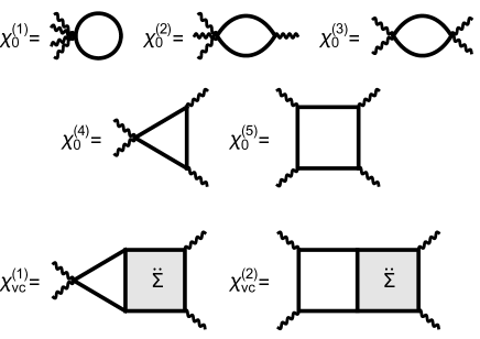
Figure 4: Feynman diagrams for the susceptibility for the third-harmonic generation. There are five (two) topologically different diagrams for the bare susceptibility $\chi_{0}$ (vertex correction $\chi_{\rm vc}$). Solid and wavy lines represent the electron and external photon propagators, respectively, while the shaded box represents the vertex correction $\ddot{\Sigma}$. Among the four photon lines, one is outgoing with an energy $3\Omega$, while the other three are incoming with an energy $\Omega$. The photon lines attached directly to the vertex are incoming.

The algorithm can be generalized to arbitrary higher-order derivatives; they are determined in turn from lower orders [$(G,\Sigma)\to(\ddot{G},\ddot{\Sigma})\to(\ddddot{G},\ddddot{\Sigma})$] due to the hierarchical structure of the dotted DMFT self-consistency defined at each derivative order. Essentially the same method has been used to evaluate the optical conductivity for periodically driven systems in Floquet DMFT,Tsuji et al. (2009) where $\dot{G}$ and $\dot{\Sigma}$ are needed. The first derivative can be nonzero, since the parity symmetry is broken by the presence of the external driving field.

So far we have formulated the dotted DMFT for the normal phase, but it is straightforward to extend the approach to the superconducting phase. There, we have to impose the following modifications: the electron Green’s functions and self-energy should be represented by $2\times 2$ matrices (Nambu-Gor’kov formalism), $\epsilon_{\bm{k}},\ddot{\epsilon}_{\bm{k}}$, and $\ddddot{\epsilon}_{\bm{k}}$ appearing in the dotted DMFT should be multiplied by $\tau_{3}$ (the third component of the Pauli matrix), and the dotted impurity solution (35) for the Holstein model should be replaced by

$$\ddot{\hat{\Sigma}}^{<,>}(t;\Omega) =ig^{2}D_{0}^{<,>}(t)\tau_{3}\ddot{\hat{G}}^{<,>}(t;\Omega)\tau_{3}.$$ (49)

Let us finally comment on the generality of the present formulation. Although we describe the dotted DMFT formulation for the THG susceptibility, it is not restricted to THG but can be generalized to arbitrary dynamical response functions. One can introduce an infinitesimal external field (not necessarily an electric field), and take the derivative with respect to it for observables. It may contain a derivative of the self-energy, which can be evaluated by the corresponding dotted DMFT, where the DMFT self-consistency equations are differentiated with respect to the external field. For example, the dynamical pair susceptibility,Cea and Benfatto (2014); Murakami et al. (2016)

$$\chi_{\rm pair}^{R}(\Omega) =-i\int_{0}^{\infty}dte^{-i\Omega t}\langle[B_{\bm{0}}(t),B_{\bm{0}}(0)]\rangle,$$ (50)

is defined as the response of the pairing amplitude $\langle B_{\bm{0}}\rangle$ against an external pair potential $H_{\rm ex}(t)=\varepsilon B_{\bm{0}}e^{-i\Omega t}$, where

$$B_{\bm{0}}=\sum_{i}(c_{i\uparrow}^{\dagger}c_{i\downarrow}^{\dagger}+c_{i\downarrow}c_{i\uparrow})$$ (51)

is the bosonic pairing operator with the center-of-mass momentum $\bm{q}=\bm{0}$. This quantity detects collective amplitude oscillations of the superconducting order parameter. The dotted DMFT is then constructed by differentiating the DMFT self-consistency with respect to the pair field potential. The resulting dotted lattice Dyson equation reads

$$\dot{\hat{G}}^{R,A,<,>}(\omega;\Omega) =\sum_{\bm{k}}\{\hat{G}_{\bm{k}}(\omega+\Omega)[\tau_{1}+\dot{\hat{\Sigma}}(\omega;\Omega)]\hat{G}_{\bm{k}}(\omega)\}^{R,A,<,>},$$ (52)

where we have adopted an extended notation of $(\tau_{1})^{R,A}=\tau_{1}$ and $(\tau_{1})^{<,>}=0$. Once the dotted DMFT is solved, the dynamical pair susceptibility can be calculated as

$$\chi_{\rm pair}^{R}(\Omega) =-i\int\frac{d\omega}{2\pi}{\rm Tr}[\tau_{1}\dot{\hat{G}}^{<}(\omega;\Omega)].$$ (53)

In the next section, we demonstrate the results obtained with the dotted DMFT for the THG susceptibility along with the dynamical pair susceptibility.

IV Results

Let us now turn to the results of the dotted DMFT for the superconducting phase of the Holstein model. The parameters are taken to be $g=0.8$, $\omega_{0}=0.6$, $\gamma=0.2$, and $\delta=0.005$. This corresponds to the effective interaction of $\lambda=0.77$ [Eq. (11)], which is in the moderately correlated regime. The temperature is set to be $T=0.02$, which is low enough for the system to be in the superconducting state. The polarization (16) is set to a general direction $\alpha=0.5$ without having a bias on the pair breaking effect.

In Fig. 5, we show the single-particle spectrum $A(\omega)=-{\rm Im}\,G_{11}^{R}(\omega)/\pi$ (red curve) along with the dynamical pair susceptibility $-{\rm Im}\,\chi_{\rm pair}^{R}(\omega)$ (50) (blue with the dots), with the latter calculated by the dotted DMFT. Previously, the dynamical pair susceptibility has been evaluated from the real-time simulation of the nonequilibrium DMFT,Murakami et al. (2016) which is one way to avoid solving the complicated Bethe-Salpeter equation for the vertex correction. Here the dotted DMFT serves as an alternative efficient method.

As one can see in Fig. 5, the single-particle spectrum shows the superconducting gap $2\Delta\approx 0.12$ [note that we plot $A(\omega/2)$ in Fig. 5] with the coherence peak at the edge of the band gap. The pair susceptibility also exhibits a clear gap structure with a resonance peak at $\omega=2\Delta$. The result is in agreement with the one previously reported.Murakami et al. (2016); Mur (b) The resonance peak is produced by the vertex correction, which is immediately confirmed by the comparison to the bare susceptibility. This suggests that the peak in $\chi_{\rm pair}^{R}(\omega)$ represents the collective oscillation of the pairing amplitude with the frequency $2\Delta$, which can be identified as the Higgs amplitude mode. The coincidence of the single-particle and two-particle gaps (up to the factor of 2) holds beyond the BCS approximation, as observed in the previous study.Murakami et al. (2016); Mur (b)

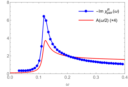
Figure 5: The single-particle spectrum $A(\omega/2)$ and the dynamical pair susceptibility $-{\rm Im}\,\chi_{\rm pair}^{R}(\omega)$ calculated by the (dotted) DMFT for the superconducting phase of the Holstein model with $g=0.8,\omega_{0}=0.6,T=0.02,\gamma=0.2$, and $\delta=0.005$.

The results of the THG susceptibility $|\chi|^{2}$ (proportional to the THG intensity observed in experiments) calculated by the dotted DMFT are plotted in Fig. 6. We show the result for each term $\chi_{0}^{(i)}$ ($i=1,\dots,5$) and $\chi_{\rm vc}^{(i)}$ ($i=1,2$). First of all, we can see that all the terms contribute to the THG response, which is in sharp contrast to the BCS approximation where $\chi_{0}^{(i)}$ ($i=2,4,5$) and $\chi_{\rm vc}^{(2)}$ identically vanish. In particular, $\chi_{0}^{(3)}$, $\chi_{0}^{(5)}$ and $\chi_{\rm vc}^{(2)}$ exhibit dominant contributions. The resonance peak exists at $\Omega=\Delta\approx 0.06$ in the spectra of $\chi_{0}^{(3)}$, $\chi_{\rm vc}^{(1)}$, and $\chi_{\rm vc}^{(2)}$. The peak in $\chi_{0}^{(3)}$ can be interpreted as individual excitations due to Cooper pair breaking, while the peaks in $\chi_{\rm vc}^{(1)}$ and $\chi_{\rm vc}^{(2)}$ can be interpreted as collective excitations resonating with the Higgs amplitude mode, since that is the only known collective mode at energy $2\Delta$. As expected from the BCS approximation,Cea et al. (2016) the effect of $\chi_{\rm vc}^{(1)}$ is a few orders of magnitude smaller than that of $\chi_{0}^{(3)}$ (see the inset of Fig. 6) if one chooses a general polarization direction (here $\alpha=0.5$). On the other hand, the contribution of $\chi_{\rm vc}^{(2)}$, which has been absent in the BCS approximation, is quite significant, and can be even larger than that of $\chi_{0}^{(3)}$. This result implies that if one resumes the factors that are not taken into account in the BCS approximation, such as the retarded nature of the pairing interaction through the electron-phonon coupling, the Higgs mode can become a prominent component in the THG spectrum. The corrections from the BCS theory are not necessarily small but can be drastic (at least when the electron-phonon coupling is large enough). Let us again recall that NbN, which is experimentally used in Refs. Matsunaga et al., 2013; Mat, , has the strong electron-phonon coupling,Kihlstrom et al. (1985); Brorson et al. (1990); Chockalingam et al. (2008) so that such corrections from the BCS analysis should be seriously taken into account. $\chi_{0}^{(5)}$ is also not negligible, but this component does not show a resonance with the Higgs mode at $\Omega=\Delta$. The increase of the spectral weight towards low frequencies (especially for $\chi_{0}^{(5)}$ and $\chi_{\rm vc}^{(2)}$) is due to the presence of nonzero $\delta$, with which the system accommodates low-energy excitations. It can be suppressed when $\delta$ is reduced, so that we can ignore the low-energy features, although we cannot take the limit of $\delta\to+0$ for the dotted DMFT to be numerically stable.

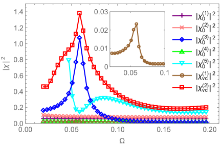
Figure 6: The THG susceptibility decomposed into the bare susceptibilities $\chi_{0}^{(i)}$ ($i=1,\dots,5$) and vertex corrections $\chi_{\rm vc}^{(i)}$ ($i=1,2$) for the superconducting phase of the Holstein model calculated with the dotted DMFT. The parameters are the same as in Fig. 5. The polarization direction of the laser field is taken to be $\alpha=0.5$. The susceptibilities are normalized by $\chi^{\ast}=t^{\ast}/d^{2}$. The inset is a blowup of $\chi_{\rm vc}^{(1)}$.

Figure 7 plots the total THG susceptibility $|\chi|^{2}=|\chi_{0}+\chi_{\rm vc}|^{2}$ as compared with the total bare susceptibility $|\chi_{0}|^{2}$. Here we subtract the low-energy increase of the spectral weight of $\chi_{0}^{(5)}$ at $\Omega<0.055$ from $\chi_{0}$, which is out of our interest and could be removed by reducing $\delta$. We can see that both $\chi$ and $\chi_{0}$ exhibit conspicuous resonance peaks at $\Omega=\Delta$. Although the position and shape of the peak do not differ so much between $\chi_{0}$ and $\chi$, the peak height does. With the parameters taken here, the height for $\chi$ is enhanced about four times that for $\chi_{0}$ due to the resonance with the Higgs mode. The main contribution comes from $\chi_{\rm vc}^{(2)}$, as can be seen in Fig. 6. The resonance width for $\chi_{0}$ is broadened as compared to that for $\chi_{0}^{(3)}$ due to the spectral weight of $\chi_{0}^{(5)}$ distributed around the peak. The amplitude ratio between $\chi_{0}$ and $\chi_{\rm vc}$ can depend on various model parameters (especially we will discuss the phonon-frequency dependence below), but at least there is such a possibility in a certain realistic parameter regime that the vertex correction has a non-negligible effect.

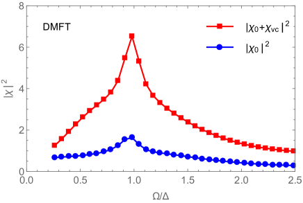
Figure 7: The intensity of the third-harmonic generation for the superconducting phase of the Holstein model calculated by the dotted DMFT. The bubble contribution ($\chi_{0}$) and the total susceptibility including the vertex corrections ($\chi_{0}+\chi_{\rm vc}$) are plotted. The parameters are taken to be the same as those of Fig. 5. The polarization direction of the laser field is taken to be $\alpha=0.5$.

We are now in position to compare the BCS and DMFT results by calculating the THG susceptibility within the BCS approximation for the same parameter set as those for DMFT. The electron-phonon coupling is translated into a static attractive interaction via $U=2g^{2}\omega_{0}/(\omega_{0}^{2}+\gamma^{2})$ [see Eqs. (9) and (10)]. In the gap equation, we perform the momentum integral in the range of $|\epsilon_{\bm{k}}|\leq\omega_{0}$. The result is displayed in Fig. 8, which indicates that the effect of the vertex correction in BCS is rather small for a general polarization direction ($\alpha=0.5$ here). The resonance width is much sharper and the peak height is higher in BCS than in DMFT, since the THG susceptibility diverges at $\Omega=\Delta$ in the limit of $\delta\to 0$ in the BCS theory. While these are consistent with the previous studies,Tsuji and Aoki (2015); Cea et al. (2016) the BCS result is markedly different from the DMFT result (Fig. 7) that takes account of dynamical correlation effects. This is simply because $\chi_{\rm vc}^{(2)}$ is absent in the BCS approximation, whereas it is generally non-negligible if one considers the retardation in the phonon-mediated interaction (or other effects that are not included in the BCS approximation such as impurity scattering, Coulomb interaction, etc.).

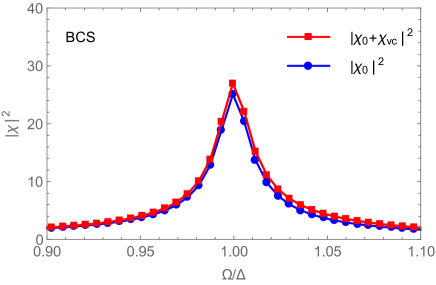
Figure 8: The intensity of the third-harmonic generation for the superconducting phase of the Holstein model calculated within the BCS approximation. The bubble contribution ($\chi_{0}$) and the total susceptibility including the vertex corrections ($\chi_{0}+\chi_{\rm vc}$) are plotted respectively. The parameters are taken to be the same as in Fig. 5. The polarization direction of the laser field is taken to be $\alpha=0.5$. Note the difference in the scales of the axes from Fig. 7.

To confirm that the retardation effect is essential in enhancing the contribution of the Higgs mode to the THG resonance, we calculate $\omega_{0}$ dependence of the THG susceptibility. Here we focus on $\chi_{0}^{(3)}(\Omega)$ and $\chi_{\rm vc}^{(2)}(\Omega)$ that are in charge of the resonance structures at $\Omega=\Delta$. A systematic comparison between the susceptibilities at different $\omega_{0}$ is made by tuning the electron-phonon coupling $g$ such that the superconducting gap is fixed to a constant ($2\Delta\approx 0.12$). In Fig. 9, we plot the height of the resonance peak for $|\chi_{0}^{(3)}(\Omega)|^{2}$ and $|\chi_{\rm vc}^{(2)}(\Omega)|^{2}$ as a function of the phonon frequency $\omega_{0}$ (with the parameters other than $\omega_{0}$ and $g$ the same as in Fig. 6). We can see that, as $\omega_{0}$ decreases and the effective interaction (9) becomes more retarded, the resonance for $\chi_{\rm vc}^{(2)}$ is enhanced while that for $\chi_{0}^{(3)}$ is suppressed. This is consistent with the expectation that in the opposite antiadiabatic (non-retarded) limit ($\omega_{0}\to\infty$) the model approaches the attractive Hubbard model, where the Migdal approximation is replaced by the BCS approximation, and $\chi_{\rm vc}^{(2)}$ vanishes as explained in Sec. I. The result suggests that the retardation effect in the electron-phonon coupling indeed plays a crucial role in amplifying the vertex correction $\chi_{\rm vc}^{(2)}$.

We can elaborate the physical meaning of the result as follows. As we discussed previously, the dominant diagrams contained in $\chi_{\rm vc}^{(2)}$ is the one with the resonant coupling to the light [Fig. 1(c)]. This represents a process in which a single photon is absorbed and then emitted by electrons at different times (with the time separation $\sim(2\Delta)^{-1}$). The retardation effect due to the scattering of phonons (in the time scale of $\omega_{0}^{-1}$) can propagate between these times. If $2\Delta$ ($\approx 0.12$ in the present case) and $\omega_{0}$ are in the same order, the scattering amplitude relevant for the THG resonance can be effectively enhanced, as confirmed from the result in Fig. 9. Note that the resonance between coherent phonons and the order parameter oscillation in the regime of $\omega_{0}\sim 2\Delta$ has been discussed in Ref. Schnyder et al., 2011.

V Summary

To summarize, we have studied the nonlinear optical response, especially the third-harmonic generation, for electron-phonon coupled superconductors by means of the dotted DMFT framework proposed in the present paper. The results show that, for general polarization of the light, there is a possibility that the Higgs amplitude mode can contribute to the THG resonance at $2\Omega=2\Delta$ with an order of magnitude comparable to contributions from the Cooper pair breaking or charge density fluctuations, which is in sharp contrast to the BCS result. The interaction between the light and Higgs mode can be mediated by the resonant coupling, which is induced by the retarded interaction through the electron-phonon coupling. This is confirmed by the observation that the intensity of the THG resonance due to the Higgs mode does indeed increase as the phonon frequency is reduced. Let us note that the electron-phonon coupling is just one of many possibilities that could enhance the Higgs-mode effect. These may include phonon renormalization, impurity scattering, dynamical correlation effects from the Coulomb interaction, non-local correlations beyond DMFT, etc.

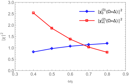
Figure 9: Phonon-frequency dependence of $|\chi_{0}^{(3)}|^{2}$ and $|\chi_{\rm vc}^{(2)}|^{2}$ at the resonance ($\Omega=\Delta$) for the superconducting phase of the Holstein model with $T=0.02$, $\gamma=0.2$, and $\delta=0.005$. The polarization direction of the laser field is taken to be $\alpha=0.5$. We tune $g$ for each $\omega_{0}$ such that the superconducting gap is fixed to a constant ($2\Delta\approx 0.12$).

To make a relevance to the experiment,Mat it is interesting to investigate temperature dependence of the THG susceptibility. However, we expect that this strongly depends on details of the model, since the model adopted here only includes a single optical phonon mode, while in realistic situations acoustic phonons may play an important role at low temperatures. The temperature dependence may also be affected by mechanisms of energy dissipation. In this paper, we have assumed a simple dissipation characterized by the broadening parameters $\gamma$ and $\delta$, but it can be more complicated in real systems. Moreover, the present method has a numerical instability when $\gamma$ or $\delta$ approaches zero. These issues will be left as a future problem. When both the pair breaking (charge fluctuation) and Higgs mode contribute with comparable magnitudes, as indicated here to be possible, it is desirable to distinguish them in experiments. One possibility is to look at the polarization dependence.Cea et al. (2016) To this end, one needs to accurately evaluate the polarization dependence of the pair breaking and Higgs-mode contributions in a realistic manner.

We wish to thank R. Shimano, R. Matsunaga, and Y. Murotani for illuminating discussions. H.A. is supported by JSPS KAKENHI (Grant No. 26247057) from MEXT and ImPACT project (No. 2015-PM12-05-01) from JST. N.T. is supported by JSPS KAKENHI Grants No. 25800192 and No. 16K17729.

Appendix A Notation for products of nonequilibrium Green’s functions

In this appendix, we explain the notation for products of nonequilibrium Green’s functions used throughout the paper. We define

$$[A(\omega)B(\omega^{\prime})]^{R,A} \equiv A^{R,A}(\omega)B^{R,A}(\omega^{\prime}),$$ (54)

$$[A(\omega)B(\omega^{\prime})]^{<,>} \equiv A^{R}(\omega)B^{<,>}(\omega^{\prime})+A^{<,>}(\omega)B^{A}(\omega^{\prime}),$$ (55)

following the Langreth rule.Lan Here $R,A,<$, and $>$ respectively denote the retarded, advanced, lesser, and greater components of nonequilibrium Green’s functions. For the detailed definition of nonequilibrium Green’s function, we refer to Ref. Aoki et al., 2014. The definition (54), (55) can be used repeatedly for products involving more than two Green’s functions. For example, it follows from the above definition that

$$[A(\omega)B(\omega^{\prime})C(\omega^{\prime\prime})]^{R,A} =A^{R,A}(\omega)B^{R,A}(\omega^{\prime})C^{R,A}(\omega^{\prime\prime}),$$ (56)

$$[A(\omega)B(\omega^{\prime})C(\omega^{\prime\prime})]^{<,>} =A^{R}(\omega)B^{R}(\omega^{\prime})C^{<,>}(\omega^{\prime\prime})$$

$$\quad+A^{R}(\omega)B^{<,>}(\omega^{\prime})C^{A}(\omega^{\prime\prime})$$

$$\quad+A^{<,>}(\omega)B^{A}(\omega^{\prime})C^{A}(\omega^{\prime\prime}).$$ (57)

If products explicitly contain $\epsilon_{\bm{k}}$, we can regard it as a component of Green’s function with the definition,

$$[\epsilon_{\bm{k}}]^{R,A} \equiv\epsilon_{\bm{k}},$$ (58)

$$[\epsilon_{\bm{k}}]^{<,>} \equiv 0.$$ (59)

For example, we have

$$[\epsilon_{\bm{k}}A(\omega)B(\omega^{\prime})]^{<,>} =\epsilon_{\bm{k}}[A^{R}(\omega)B^{<,>}(\omega^{\prime})+A^{<,>}(\omega)B^{A}(\omega^{\prime})].$$ (60)

The same applies to derivatives of $\epsilon_{\bm{k}}$ such as $\dot{\epsilon}_{\bm{k}},\ddot{\epsilon}_{\bm{k}}$.

Appendix B A momentum integral formula for the calculation of THG

In this appendix, we summarize some useful formulae for the momentum integral employed in the calculation of the THG susceptibility in the dotted DMFT. As we have seen in Sec. III, one frequently encounters a momentum integral of a function of $\epsilon_{\bm{k}}$ [Eq. (8)] multiplied by some of $\dot{\epsilon}_{\bm{k}},\ddot{\epsilon}_{\bm{k}},\dddot{\epsilon}_{\bm{k}}$, and $\ddddot{\epsilon}_{\bm{k}}$ [see Eqs. (19)-(20) for the definition]. In the main text, we have taken the polarization vector as

$$\bm{e} =\frac{1}{\sqrt{m}}(\overbrace{\underbrace{1,1,\dots,1}_{m},0,\dots,0}^{d}).$$ (61)

In the limit $d,m\to\infty$ with a fixed ratio $\alpha=m/d$, the momentum integral is reduced to an integral over the single variable $\epsilon=\epsilon_{\bm{k}}$, as described in Sec. II.

Here we list the results. For momentum integrals containing two derivatives, we have

$$\sum_{\bm{k}}\ddot{\epsilon}_{\bm{k}}f(\epsilon_{\bm{k}}) =-\frac{1}{d}\sum_{\bm{k}}\epsilon_{\bm{k}}f(\epsilon_{\bm{k}}),$$ (62)

$$\sum_{\bm{k}}(\dot{\epsilon}_{\bm{k}})^{2}f(\epsilon_{\bm{k}}) =\frac{t^{\ast}{}^{2}}{d}\sum_{\bm{k}}f(\epsilon_{\bm{k}}),$$ (63)

which can be used in the calculation of $\chi_{\rm vc}^{(i)}$ [Eqs. (47)-(48)] and the dotted lattice Dyson equation (31). For momentum integrals containing four derivatives, we have

$$\sum_{\bm{k}}\ddddot{\epsilon}_{\bm{k}}f(\epsilon_{\bm{k}}) =\frac{1}{d^{2}\alpha}\sum_{\bm{k}}\epsilon_{\bm{k}}f(\epsilon_{\bm{k}}),$$ (64)

$$\sum_{\bm{k}}\dot{\epsilon}_{\bm{k}}\dddot{\epsilon}_{\bm{k}}f(\epsilon_{\bm{k}}) =-\frac{t^{\ast}{}^{2}}{d^{2}\alpha}\sum_{\bm{k}}f(\epsilon_{\bm{k}}),$$ (65)

$$\sum_{\bm{k}}(\ddot{\epsilon}_{\bm{k}})^{2}f(\epsilon_{\bm{k}}) =\frac{t^{\ast}{}^{2}(1-\alpha)}{d^{2}\alpha}\sum_{\bm{k}}f(\epsilon_{\bm{k}})+\frac{1}{d^{2}}\sum_{\bm{k}}\epsilon_{\bm{k}}^{2}f(\epsilon_{\bm{k}}),$$ (66)

$$\sum_{\bm{k}}(\dot{\epsilon}_{\bm{k}})^{2}\ddot{\epsilon}_{\bm{k}}f(\epsilon_{\bm{k}}) =-\frac{t^{\ast}{}^{2}}{d^{2}}\sum_{\bm{k}}\epsilon_{\bm{k}}f(\epsilon_{\bm{k}}),$$ (67)

$$\sum_{\bm{k}}(\dot{\epsilon}_{\bm{k}})^{4}f(\epsilon_{\bm{k}}) =\frac{3t^{\ast}{}^{4}}{d^{2}}\sum_{\bm{k}}f(\epsilon_{\bm{k}}),$$ (68)

which can be used in the calculation of $\chi_{0}^{(i)}$ [Eqs. (42)-(46)].

Once the momentum integral is reduced to an integral over $\epsilon=\epsilon_{\bm{k}}$, it can be further evaluated analytically. To see this, let us parametrize the self-energy (at half filling with $\mu=0$) as

$$\hat{\Sigma}^{R}(\omega) =[1-Z(\omega)]\omega+\phi(\omega)\tau_{1}.$$ (69)

We define functions

$$\hat{S}^{\pm}(\omega) \equiv Z(\omega)\omega\pm\phi(\omega)\tau_{1},$$ (70)

$$S^{2}(\omega) \equiv[Z(\omega)\omega]^{2}-\phi(\omega)^{2},$$ (71)

with which the retarded Green’s function is represented as

$$\hat{G}_{\bm{k}}^{R}(\omega) =[\omega-\epsilon_{\bm{k}}\tau_{3}-\hat{\Sigma}^{R}(\omega)]^{-1}=\frac{\hat{S}^{+}(\omega)+\epsilon_{\bm{k}}\tau_{3}}{S^{2}(\omega)-\epsilon_{\bm{k}}^{2}}.$$ (72)

As an example, let us consider the first term in the dotted lattice Dyson equation (31), whose retarded component can be evaluated with Eq. (62) as

$$\sum_{\bm{k}}\hat{G}_{\bm{k}}^{R}(\omega+2\Omega)\ddot{\epsilon}_{\bm{k}}\tau_{3}\hat{G}_{\bm{k}}^{R}(\omega)$$

$$=-\frac{1}{d}\sum_{\bm{k}}\frac{\hat{S}^{+}(\omega+2\Omega)+\epsilon_{\bm{k}}\tau_{3}}{S^{2}(\omega+2\Omega)-\epsilon_{\bm{k}}^{2}}\epsilon_{\bm{k}}\tau_{3}\frac{\hat{S}^{+}(\omega)+\epsilon_{\bm{k}}\tau_{3}}{S^{2}(\omega)-\epsilon_{\bm{k}}^{2}}$$

$$=\frac{1}{d}\frac{\hat{G}^{R}(\omega)\hat{S}^{-}(\omega)-\hat{G}^{R}(\omega+2\Omega)\hat{S}^{-}(\omega+2\Omega)}{S^{2}(\omega)-S^{2}(\omega+2\Omega)}$$

$$\quad\times[\hat{S}^{+}(\omega)+\hat{S}^{+}(\omega+2\Omega)].$$ (73)

Note that $\hat{G}^{R}(\omega)$ and $\hat{S}^{\pm}(\omega^{\prime})$ commute with each other. In this way, every momentum integral appearing in the calculation of the dotted DMFT and nonlinear optical susceptibilities can be written in terms of the local Green’s function and self-energy. This greatly reduces the computational cost of the dotted DMFT algorithm.

References

- Fausti et al. (2011) D. Fausti, R. I. Tobey, N. Dean, S. Kaiser, A. Dienst, M. C. Hoffmann, S. Pyon, T. Takayama, H. Takagi, and A. Cavalleri, Science 331, 189 (2011).
- Cortés et al. (2011) R. Cortés, L. Rettig, Y. Yoshida, H. Eisaki, M. Wolf, and U. Bovensiepen, Phys. Rev. Lett. 107, 097002 (2011).
- Smallwood et al. (2012) C. L. Smallwood, J. P. Hinton, C. Jozwiak, W. Zhang, J. D. Koralek, H. Eisaki, D.-H. Lee, J. Orenstein, and A. Lanzara, Science 336, 1137 (2012).
- Dal Conte et al. (2012) S. Dal Conte, C. Giannetti, G. Coslovich, F. Cilento, D. Bossini, T. Abebaw, F. Banfi, G. Ferrini, H. Eisaki, M. Greven, et al., Science 335, 1600 (2012).
- Kaiser et al. (2014) S. Kaiser, C. R. Hunt, D. Nicoletti, W. Hu, I. Gierz, H. Y. Liu, M. Le Tacon, T. Loew, D. Haug, B. Keimer, et al., Phys. Rev. B 89, 184516 (2014).
- Matsunaga and Shimano (2012) R. Matsunaga and R. Shimano, Phys. Rev. Lett. 109, 187002 (2012).
- Hinton et al. (2013) J. P. Hinton, J. D. Koralek, G. Yu, E. M. Motoyama, Y. M. Lu, A. Vishwanath, M. Greven, and J. Orenstein, Phys. Rev. Lett. 110, 217002 (2013).
- (8) B. Mansart, J. Lorenzana, A. Mann, A. Odeh, M. Scarongella, M. Chergui, and F. Carbone, Proc. Natl. Acad. Sci. 110, 4539 (2013).
- Matsunaga et al. (2013) R. Matsunaga, Y. I. Hamada, K. Makise, Y. Uzawa, H. Terai, Z. Wang, and R. Shimano, Phys. Rev. Lett. 111, 057002 (2013).
- Hu et al. (2014) W. Hu, S. Kaiser, D. Nicoletti, C. R. Hunt, I. Gierz, M. C. Hoffmann, M. Le Tacon, T. Loew, B. Keimer, and A. Cavalleri, Nat. Mater. 13, 705 (2014).
- Mankowsky et al. (2014) R. Mankowsky, A. Subedi, M. Forst, S. O. Mariager, M. Chollet, H. T. Lemke, J. S. Robinson, J. M. Glownia, M. P. Minitti, A. Frano, et al., Nature 516, 71 (2014).
- (12) R. Matsunaga, N. Tsuji, H. Fujita, A. Sugioka, K. Makise, Y. Uzawa, H. Terai, Z. Wang, H. Aoki, and R. Shimano, Science 345, 1145 (2014).
- Mitrano et al. (2016) M. Mitrano, A. Cantaluppi, D. Nicoletti, S. Kaiser, A. Perucchi, S. Lupi, P. Di Pietro, D. Pontiroli, M. Riccò, S. R. Clark, et al., Nature 530, 461 (2016).
- Giannetti et al. (2016) C. Giannetti, M. Capone, D. Fausti, M. Fabrizio, F. Parmigiani, and D. Mihailovic, Adv. Phys. 65, 58 (2016).
- Anderson (1958) P. W. Anderson, Phys. Rev. 112, 1900 (1958).
- (16) Y. Nambu and G. Jona-Lasinio, Phys. Rev. 122, 345 (1961).
- Anderson (1963) P. W. Anderson, Phys. Rev. 130, 439 (1963).
- (18) F. Englert and R. Brout, Phys. Rev. Lett. 13 321, (1964).
- (19) P. W. Higgs, Phys. Lett. 12, 132 (1964); Phys. Rev. Lett. 13, 508 (1964).
- (20) G. S. Guralnik, C. R. Hagen, and T. W. B. Kibble, Phys. Rev. Lett. 13, 585 (1964).
- Vol (a) A. F. Volkov and S. M. Kogan, Sov. Phys. JETP 38, 1018 (1974).
- (22) P. B. Littlewood and C. M. Varma, Phys. Rev. Lett. 47, 811 (1981); Phys. Rev. B 26, 4883 (1982).
- (23) I. O. Kulik, O. Entin-Wohlman, and R. Orbach, J. Low Temp. Phys. 43, 591 (1981).
- Varma (2002) C. Varma, J. Low Temp. Phys. 126, 901 (2002).
- Barankov et al. (2004) R. A. Barankov, L. S. Levitov, and B. Z. Spivak, Phys. Rev. Lett. 93, 160401 (2004).
- Yuzbashyan et al. (2006) E. A. Yuzbashyan, O. Tsyplyatyev, and B. L. Altshuler, Phys. Rev. Lett. 96, 097005 (2006).
- Barankov and Levitov (2006) R. A. Barankov and L. S. Levitov, Phys. Rev. Lett. 96, 230403 (2006).
- Yuzbashyan and Dzero (2006) E. A. Yuzbashyan and M. Dzero, Phys. Rev. Lett. 96, 230404 (2006).
- Papenkort et al. (2007) T. Papenkort, V. M. Axt, and T. Kuhn, Phys. Rev. B 76, 224522 (2007).
- Papenkort et al. (2008) T. Papenkort, T. Kuhn, and V. M. Axt, Phys. Rev. B 78, 132505 (2008).
- Gurarie (2009) V. Gurarie, Phys. Rev. Lett. 103, 075301 (2009).
- Schnyder et al. (2011) A. P. Schnyder, D. Manske, and A. Avella, Phys. Rev. B 84, 214513 (2011).
- Podolsky et al. (2011) D. Podolsky, A. Auerbach, and D. P. Arovas, Phys. Rev. B 84, 174522 (2011).
- Vol (b) G. E. Volovik and M. A. Zubkov, Phys. Rev. D 87, 075016 (2013); J. Low Temp. Phys. 175, 486 (2014).
- Tsuji et al. (2013) N. Tsuji, M. Eckstein, and P. Werner, Phys. Rev. Lett. 110, 136404 (2013).
- Barlas and Varma (2013) Y. Barlas and C. M. Varma, Phys. Rev. B 87, 054503 (2013).
- Tsuchiya et al. (2013) S. Tsuchiya, R. Ganesh, and T. Nikuni, Phys. Rev. B 88, 014527 (2013).
- Gazit et al. (2013) S. Gazit, D. Podolsky, and A. Auerbach, Phys. Rev. Lett. 110, 140401 (2013).
- Krull et al. (2014) H. Krull, D. Manske, G. S. Uhrig, and A. P. Schnyder, Phys. Rev. B 90, 014515 (2014).
- Cea and Benfatto (2014) T. Cea and L. Benfatto, Phys. Rev. B 90, 224515 (2014).
- Pekker and Varma (2015) D. Pekker and C. Varma, Annu. Rev. Condens. Matter Phys. 6, 269 (2015).
- Kemper et al. (2015) A. F. Kemper, M. A. Sentef, B. Moritz, J. K. Freericks, and T. P. Devereaux, Phys. Rev. B 92, 224517 (2015).
- Cea et al. (2015) T. Cea, C. Castellani, G. Seibold, and L. Benfatto, Phys. Rev. Lett. 115, 157002 (2015).
- Tsuji and Aoki (2015) N. Tsuji and H. Aoki, Phys. Rev. B 92, 064508 (2015).
- Peronaci et al. (2015) F. Peronaci, M. Schiró, and M. Capone, Phys. Rev. Lett. 115, 257001 (2015).
- Jujo (2015) T. Jujo, J. Phys. Soc. Jpn 84, 114711 (2015).
- (47) H. Krull, N. Bittner, G. S. Uhrig, D. Manske, and A. P. Schnyder, arXiv:1512.08121.
- Murakami et al. (2016) Y. Murakami, P. Werner, N. Tsuji, and H. Aoki, Phys. Rev. B 93, 094509 (2016).
- Cea et al. (2016) T. Cea, C. Castellani, and L. Benfatto, Phys. Rev. B 93, 180507 (2016).
- Mur (a) Y. Murotani, N. Tsuji, and H. Aoki, arXiv:1511.05762.
- Mur (b) Y. Murakami, P. Werner, N. Tsuji, and H. Aoki, arXiv:1604.08073.
- Sooryakumar and Klein (1980) R. Sooryakumar and M. V. Klein, Phys. Rev. Lett. 45, 660 (1980).
- Méasson et al. (2014) M.-A. Méasson, Y. Gallais, M. Cazayous, B. Clair, P. Rodière, L. Cario, and A. Sacuto, Phys. Rev. B 89, 060503 (2014).
- (54) D. C. Langreth, in Linear and Nonlinear Electron Transport in Solids, edited by J. T. Devreese and V. E. van Doren (Plenum Press, New York, 1976).
- Kihlstrom et al. (1985) K. E. Kihlstrom, R. W. Simon, and S. A. Wolf, Phys. Rev. B 32, 1843 (1985).
- Brorson et al. (1990) S. D. Brorson, A. Kazeroonian, J. S. Moodera, D. W. Face, T. K. Cheng, E. P. Ippen, M. S. Dresselhaus, and G. Dresselhaus, Phys. Rev. Lett. 64, 2172 (1990).
- Chockalingam et al. (2008) S. P. Chockalingam, M. Chand, J. Jesudasan, V. Tripathi, and P. Raychaudhuri, Phys. Rev. B 77, 214503 (2008).
- Devereaux and Hackl (2007) T. P. Devereaux and R. Hackl, Rev. Mod. Phys. 79, 175 (2007).
- Butcher and Cotter (1998) P. N. Butcher and D. Cotter, The Elements of Nonlinear Optics (Cambridge University Press, Cambridge, England, 1998).
- Zimmermann et al. (1991) W. Zimmermann, E. Brandt, M. Bauer, E. Seider, and L. Genzel, Physica C: Supercond. 183, 99 (1991).
- Shvaika et al. (2004) A. M. Shvaika, O. Vorobyov, J. K. Freericks, and T. P. Devereaux, Phys. Rev. Lett. 93, 137402 (2004).
- Shvaika et al. (2005) A. M. Shvaika, O. Vorobyov, J. K. Freericks, and T. P. Devereaux, Phys. Rev. B 71, 045120 (2005).
- Georges et al. (1996) A. Georges, G. Kotliar, W. Krauth, and M. J. Rozenberg, Rev. Mod. Phys. 68, 13 (1996).
- Freericks and Zlatić (2003) J. K. Freericks and V. Zlatić, Rev. Mod. Phys. 75, 1333 (2003).
- Matveev et al. (2010) O. P. Matveev, A. M. Shvaika, and J. K. Freericks, Phys. Rev. B 82, 155115 (2010).
- Jujo (2006) T. Jujo, J. Phys. Soc. Jpn 75, 104709 (2006).
- Jujo (2008) T. Jujo, J. Phys. Soc. Jpn 77, 064703 (2008).
- Jujo (2009) T. Jujo, J. Phys. Soc. Jpn 78, 044707 (2009).
- Mizuno et al. (2000) Y. Mizuno, K. Tsutsui, T. Tohyama, and S. Maekawa, Phys. Rev. B 62, R4769 (2000).
- Takahashi et al. (2002) M. Takahashi, T. Tohyama, and S. Maekawa, Phys. Rev. B 66, 125102 (2002).
- Kemper et al. (2013) A. F. Kemper, B. Moritz, J. K. Freericks, and T. P. Devereaux, New J. Phys. 15, 023003 (2013).
- Sota et al. (2015) S. Sota, S. Yunoki, and T. Tohyama, J. Phys. Soc. Jpn 84, 054403 (2015).
- (73) N. Tsuji, Ph.D. thesis, University of Tokyo (2011).
- Aoki et al. (2014) H. Aoki, N. Tsuji, M. Eckstein, M. Kollar, T. Oka, and P. Werner, Rev. Mod. Phys. 86, 779 (2014).
- Metzner and Vollhardt (1989) W. Metzner and D. Vollhardt, Phys. Rev. Lett. 62, 324 (1989).
- Murakami et al. (2015) Y. Murakami, P. Werner, N. Tsuji, and H. Aoki, Phys. Rev. B 91, 045128 (2015).
- Caldeira and Leggett (1983) A. Caldeira and A. Leggett, Ann. Phys. 149, 374 (1983).
- Tsuji et al. (2009) N. Tsuji, T. Oka, and H. Aoki, Phys. Rev. Lett. 103, 047403 (2009).
- Turkowski and Freericks (2005) V. Turkowski and J. K. Freericks, Phys. Rev. B 71, 085104 (2005).
- Tsuji et al. (2008) N. Tsuji, T. Oka, and H. Aoki, Phys. Rev. B 78, 235124 (2008).
- (81) M. A. Sentef, A. F. Kemper, A. Georges, and C. Kollath, arXiv:1505.07575.
- Kishida et al. (2000) H. Kishida, H. Matsuzaki, H. Okamoto, T. Manabe, M. Yamashita, Y. Taguchi, and Y. Tokura, Nature 405, 929 (2000).
- Kishida et al. (2001) H. Kishida, M. Ono, K. Miura, H. Okamoto, M. Izumi, T. Manako, M. Kawasaki, Y. Taguchi, Y. Tokura, T. Tohyama, et al., Phys. Rev. Lett. 87, 177401 (2001).
- Georges and Kotliar (1992) A. Georges and G. Kotliar, Phys. Rev. B 45, 6479 (1992).