Large Antenna Analysis of Multi-Cell Full-Duplex Networks

Abstract

We study a multi-cell multi-user MIMO full-duplex network, where each base station (BS) has multiple antennas with full-duplex capability supporting single-antenna users with either full-duplex or half-duplex radios. We characterize the up- and downlink ergodic achievable rates for the case of linear precoders and receivers. The rate analysis includes practical constraints such as imperfect self-interference cancellation, channel estimation error, training overhead and pilot contamination. We show that the 2$\times$ gain of full-duplex over half-duplex system remains in the asymptotic regime where the number of BS antennas grows infinitely large. We numerically evaluate the finite SNR and antenna performance, which reveals that full-duplex networks can use significantly fewer antennas to achieve spectral efficiency gain over the half-duplex counterparts. In addition, the overall full-duplex gains can be achieved under realistic 3GPP multi-cell network settings despite the increased interference introduced in the full-duplex networks.

I Introduction

One of the emerging techniques to significantly improve the spectral efficiency in wireless networks is full-duplex wireless communication [1]. In-band full-duplex wireless allows simultaneous transmission and reception using the same frequency band, and thus opens up new design opportunities to increase the spectral efficiency of wireless systems. The feasibility of a (near-)full-duplex radio has been demonstrated by many groups, see e.g.[1, 2, 3, 4, 5, 6, 7] and references therein. A side-effect of the full-duplex operation is that additional interference is introduced because there are more simultaneous active links and hence there is a possibility that the full-duplex gain can be offset by the loss due to additional interference. In the example shown in Fig. 1, the uplink rate will be affected by the new interference from neighboring full-duplex BSs, and downlink rate will be affected by the new interference from uplink users (UE).

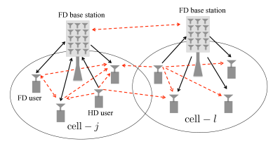
Figure 1: The full-duplex BS in each cell has $M$ antennas, and the UE has single antenna with either full-duplex or half-duplex radio. Besides the conventional interference, there will be new BS-BS and UE-UE interference highlighted by the red dash lines.

In this paper, we study if and how large antenna arrays at BSs can be used to manage the increased intra- and inter-cell interference in full-duplex enabled networks. Recently, the use of a very large antenna array at the BS has become very attractive [8, 9, 10], known as massive MIMO, where a BS has orders of magnitude more antennas compared with the current use. The large antenna array at the BS not only can increase the network capacity many-fold, but also enable a new network architecture to simplify baseband signal processing [8], eliminate inter-cell interference [11], and reduce node transmit power for energy saving [12]. The experimental evidence on the benefits of massive MIMO has already sparked strong industry interest and 64-antenna configuration [13] is now being considered for 5G systems.

Our contributions are three-fold. First, we provide a general analysis to characterize the uplink and downlink ergodic achievable rates in multi-cell multi-user MIMO (MU-MIMO) full-duplex networks. Focusing on computationally efficient linear receivers and precoders, we consider the case where each BS has multiple antennas with full-duplex capability, while each UE has a single antenna with either full-duplex or half-duplex radio. Practical constraints such as imperfect self-interference cancellation, channel estimation error, training overhead and pilot contamination are considered in our analysis.

Second, we analyze the system performance in the asymptotic regime where the number of BS antennas grows infinitely large. We show that the transmit power of BSs and UEs can be scaled down with an increasing number of BS antennas to maintain a fixed asymptotic rate. The impact of imperfect self-interference cancellation at full-duplex BSs and full-duplex UEs, intra-cell and inter-cell interference in the multi-cell MU-MIMO full-duplex networks disappears as the number of BS antennas becomes infinitely large. Under the assumption of perfect channel knowledge, full-duplex system asymptotically achieves 2$\times$ spectral efficiency gain over the half-duplex system. When channel estimation error and channel training overhead are considered, the 2$\times$ asymptotic full-duplex gain is achieved when serving only full-duplex UEs.

Lastly, we numerically evaluate the system performance in finite SNR and finite antenna regimes. Our numerical results reveal that full-duplex networks can use significantly fewer antennas to achieve spectral efficiency gain over the half-duplex counterparts. In addition, under realistic 3GPP multi-cell network scenarios [14], the overall full-duplex gains can be achieved despite the increased interference introduced in the full-duplex networks.

Related work: There are two lines of work in the area of MU-MIMO full-duplex cellular networks. The first line of work focuses on information theoretic limits while the other line of work focuses on practical network design. Towards that end, we discuss [15, 16, 17, 18, 19, 20, 21, 22, 23]; note that not all papers are multi-cell studies. In [15, 16, 17, 18, 19], only a single-cell MIMO full-duplex case is studied. The authors in [15, 16, 17] study the information theoretic limits of a single-cell MU-MIMO full-duplex network, where the high signal-to-noise (SNR) approximation, i.e., degrees of freedom or multiplexing gains have been characterized. In [18, 19], the authors propose opportunistic scheduling and a distributed power control method to mitigate UE-UE interference in a single-cell MIMO full-duplex network. Authors in [20] present several schemes to manage UE-UE interference via out-of-band wireless side-channels in the full-duplex network.

All the papers [21, 22, 23] study multi-cell full-duplex networks. In [21], scheduling and power control algorithms with BS cooperation in the multi-cell SISO full-duplex networks are investigated and [22] studies the MIMO case with 4 BS antennas. The performance analyses are based on extensive simulations, largely because of the challenge of analyzing complex scheduling and power control methods. In [23], the authors study the degrees of freedom region when the BSs have full coordination. This converts the problem into a network MIMO problem, and essentially allows one to treat the multi-cell problem as one giant MIMO cell. This, in turn, allows the use of interference alignment to achieve the highest possible degrees of freedom. While this approach provides insights into the maximum possible degrees of freedom, it relies on full coordination and proposes a very complex transmission method - both of them are extremely challenging to implement in practice. Compared to the above works, we focus on the case when there is no BS coordination and hence we cannot convert the problem to the more tractable single-cell problem. In addition, we allow only simple linear processing at the BSs, namely conjugate beamforming, and hence complex schemes like zero-forcing or interference-alignment cannot be employed.

The rest of paper is organized as follows. We first describe the system model in Section II. In Section III, we characterize the ergodic achievable rates of uplink and downlink under both perfect and imperfect CSI assumptions. The large-scale system performance is studied in Section LABEL:asym. The numerical results with realistic network evaluation are presented in Section V. Section VI concludes the paper.

II Multi-cell Full-Duplex System Model

We consider a multi-cell MU-MIMO full-duplex system with $L~{}(\geq 1)$ cells, where each cell has one in-band full-duplex BS with $M$ antennas. In each cell, single-antenna UEs with either full-duplex or half-duplex radios are supported. Each BS can serve $K_{f}$ full-duplex (FD) users, $K_{h}^{u}$ half-duplex (HD) uplink users and $K_{h}^{d}$ half-duplex downlink users. We denote $\mathcal{K}_{u}=\{\underbrace{1,\cdots,K_{f}}_{\mathrm{FD~{}UE}},\underbrace{K_{f}+1,\cdots,K_{f}+K_{h}^{u}}_{\mathrm{HD~{}UE}}\}$ as the set of all uplink users, where the first $K_{f}$ elements represent $K_{f}$ full-duplex users; and the last $K_{h}^{u}$ elements represent half-duplex uplink users. The set of all downlink users are denoted as $\mathcal{K}_{d}=\{\underbrace{1,\cdots,K_{f}}_{\mathrm{FD~{}UE}},\underbrace{K_{f}+1,\cdots,K_{f}+K_{h}^{d}}_{\mathrm{HD~{}UE}}\}$, where the first $K_{f}$ elements represent full-duplex users, and the last $K_{h}^{d}$ elements represent half-duplex downlink users. We further denote the set of full-duplex users as $\mathcal{K}_{f}\triangleq\{1,\cdots,K_{f}\}$ and set of half-duplex downlink users as $\mathcal{K}_{h}^{d}\triangleq\{K_{f}+1,\cdots,K_{f}+K_{h}^{d}\}$. The total number of uplink users is $|\mathcal{K}_{u}|\triangleq K_{u}$, where $K_{u}=K_{f}+K_{h}^{u}$ and the total number of downlink users is $|\mathcal{K}_{d}|\triangleq K_{d}$, where $K_{d}=K_{f}+K_{h}^{d}$.

The uplink and downlink data are transmitted over the same time-frequency slot with block fading. The analysis in this paper can be applied to wide-band channels like OFDM system.

In this work, we will consider practical constraints on the full-duplex radio chains such as non-ideal power amplifier, oscillator phase noise, non-ideal digital-to-analog converter and analog-to-digital converter, which can be captured by the dynamic range model [24, 25]. The dynamic range model approximates the imperfect full-duplex transmit radio chain as an additive white Gaussian “transmitter noise” added to each transmit antenna. The variance of the transmitter noise is $\kappa$ ($\kappa\ll 1$) times the power of the transmit signals, where $\kappa$ is the dynamic range parameter. The full-duplex transmitter noise will propagate over the self-interference (SI) channel and become nontrivial compared to the receiver thermal noise. However, the effect of transmitter noise that propagates over the uplink/downlink channels can be ignored compared to the receiver thermal noise [25].

II-A Uplink

The $j$-th full-duplex BS will receive an $M\times 1$ uplink signal vector $\bm{y}_{u,j}^{\prime}$:

$$\begin{aligned} \bm{y}_{u,j}^{\prime}=\sum_{l=1}^{L}\bm{G}_{u,jl}\bm{x}_{u,l}+\sum_{l=1}^{L}\bm{V}_{jl}\bm{x}_{d,l}+\bm{V}_{jj}\bm{e}_{bs,j}+\bm{n}_{u,j},\end{aligned}$$ (1)

where $\bm{x}_{u,l}=\sqrt{P_{u}}\bm{u}_{l}$ denotes the uplink transmit signal vector, $\bm{u}_{l}\triangleq[u_{l,1},\cdots,u_{l,K_{u}}]^{T}$ is a $K_{u}\times 1$ vector consisting of uplink messages of the $K_{u}$ uplink users in the $l$-th cell. Each user has an average power constraint $P_{u}$, and $\mathbb{E}(|{u}_{l,k}|^{2})=1$, for $k\in\mathcal{K}_{u}$. $\bm{x}_{d,l}$ is an $M\times 1$ vector denoting downlink transmit signal in the $l$-th cell. Each BS has an average power constraint $P_{d}$.

We assume $\bm{G}_{u,jl}$ is an $M\times K_{u}$ matrix denoting the channel between the uplink users in the $l$-th cell and the $j$-th BS. The propagation channel model in our system considers both small-scale fading due to mobility and multipath, and large-scale fading due to geometric attenuation and shadowing effect, thus allowing arbitrary cell layout.

The uplink channel $\bm{G}_{u,jl}$ encompasses independent small-scale fading and large-scale fading

$$(\bm{G}_{u,jl})_{m,n}\triangleq g_{u,jmln}=h_{u,jmln}\sqrt{\beta_{u,jln}},$$

where $j,l\in\{1,\cdots,L\},m\in\{1,\cdots,M\},n\in\mathcal{K}_{u}$. $h_{u,jmln}$ is the small-scale fading value between the $n$-th uplink user in the $l$-th cell and the $m$-th antenna at the $j$-th BS, following independent and identically distributed (i.i.d.) circularly-symmetric complex Gaussian distribution $\mathcal{CN}(0,1)$. We use ${\beta_{u,jln}}$ to model the path loss and shadow fading between the $n$-th uplink user in the $l$-th cell and the $j$-th BS, which is independent of $m$. Such long-term parameters can be measured at the BS.

The BS-BS channel $\bm{V}_{j,l}$ is an $M\times M$ matrix denoting the channel between the $l$-th BS and the $j$-th BS, and $\bm{V}_{j,j}$ denotes the SI channel for the $j$-th full-duplex BS. We assume $\bm{V}_{j,l}$ contains i.i.d $\mathcal{CN}(0,\beta_{b,jl})$ elements. The imperfect full-duplex transmit front-end chain is modeled as transmit noise $\bm{e}_{bs,j}\in\mathbb{C}^{M\times 1}$ added to each transmit antenna at the $j$-th full-duplex BS. And $\bm{e}_{bs,j}$ will propagate through the SI channel and follow $\mathcal{CN}\left(0,\frac{\kappa P_{d}}{M}\bm{I}_{M}\right)$ assuming equal power allocation among downlink users, where $\bm{I}_{M}$ denotes an $M\times M$ identity matrix. The receiver thermal noise is denoted as $\bm{n}_{u,j}$ which contains i.i.d $\mathcal{CN}(0,\sigma^{2})$ entries.

The $j$-th BS then performs SI cancellation by knowing its SI channel and its downlink signal. Hence from (1), we have

$$\begin{aligned} \bm{y}_{u,j}=\sum_{l=1}^{L}\bm{G}_{u,jl}\bm{x}_{u,l}+\sum_{l\neq j}^{L}\bm{V}_{j,l}\bm{x}_{d,l}+\bm{z}_{u,j},\end{aligned}$$ (2)

where $\bm{z}_{u,j}\sim\mathcal{CN}\left(0,\left(\sigma^{2}+\kappa P_{d}\beta_{b,jj}\right)\bm{I}_{M}\right)$.

II-B Downlink

The received signals for the $K_{d}$ downlink users in the $l$-th cell can be expressed as a $K_{d}\times 1$ vector $\bm{y}_{d,l}$, given by

$$\begin{aligned} \bm{y}_{d,l}=\sum_{j=1}^{L}\bm{G}^{T}_{d,jl}\bm{x}_{d,j}+\sum_{j=1}^{L}\bm{F}_{lj}\bm{x}_{u,j}+\bm{J}_{l}+\bm{n}_{d,l},\end{aligned}$$ (3)

where $\bm{G}_{d,jl}$ is an $M\times K_{d}$ matrix denoting the channel between the downlink users in the $l$-th cell and the $j$-th BS, the downlink channel can be represented as $\bm{G}_{d,jl}^{T}$ and we have

$$(\bm{G}_{d,jl})_{m,k}^{T}\triangleq g^{T}_{d,jmlk}=h^{T}_{d,jmlk}\sqrt{\beta_{d,jlk}},$$

where $k\in\mathcal{K}_{d}$, the superscript $``T"$ denotes transpose. $h_{d,jmlk}$ is the small-scale fading value between the $k$-th downlink user in the $l$-th cell and the $m$-th antenna at the $j$-th BS, following $\mathcal{CN}(0,1)$; ${\beta_{d,jlk}}$ incorporates path loss and shadow fading between the $k$-th downlink user in the $l$-th cell and the $j$-th BS .

The UE-UE interference channel $\bm{F}_{lj}$ is a $K_{d}\times K_{u}$ matrix denoting the interference channel from $K_{u}$ uplink users in the $j$-th to $K_{d}$ downlink users in the $l$-th cell; $\bm{J}_{l}=\begin{pmatrix}\mathsf{diag}(\bm{S}_{ll})\bm{e}_{ue,l}\\ \bm{0}\end{pmatrix}$ is a $K_{d}\times 1$ vector, where $\bm{S}_{ll}$ is a $K_{f}\times K_{f}$ matrix denoting the interference channels between full-duplex users in the $l$-th cell. The diagonal elements of $\bm{S}_{ll}$ constitute SI channels for each full-duplex user in the $l$-th cell. And $\bm{S}_{ll}$ is a sub-matrix of $\bm{F}_{ll}$, where $\left(\mathsf{diag}(\bm{S}_{ll})\right)_{k}=(\bm{F}_{ll})_{k,k}\triangleq f_{lklk},~{}k\in\mathcal{K}_{f}$. We assume each entry in $(\bm{F}_{lj})_{k,n}\triangleq f_{lkjn}$ models both the large-scale and fast fading channel coefficient between the $n$-th uplink user in the $j$-th cell and the $k$-th downlink user in the $l$-th cell, and follows i.i.d. $\sim\mathcal{CN}(0,\beta_{I,lkjn})$, where $j,l\in\{1,\cdots,L\}$ and $n\in\mathcal{K}_{u},k\in\mathcal{K}_{d}$. The transmit noise at each full-duplex user in the $l$-th cell $\bm{e}_{ue,l}\in\mathbb{C}^{K_{f}\times 1}$ will propagate through the SI channel and follow $\mathcal{CN}\left(0,\kappa P_{u}\bm{I}_{K_{f}}\right)$. The receiver thermal noise $\bm{n}_{d,l}$ follows $\sim\mathcal{CN}(0,\sigma^{2}\bm{I}_{K_{d}})$.

Next, the $k$-th full-duplex user in the $l$-th cell where $k\in\mathcal{K}_{f}$, will perform SI cancellation by subtracting out its own interference from the received signal in (3). Thus we have where $\bm{g}_{d,jlk}$ is the $k$-th column of matrix $\bm{G}_{d,jl}$ and ${z}_{d,lk}\sim\mathcal{CN}\left(0,\left(\sigma^{2}+\kappa P_{u}\beta_{I,lklk}\right)\right).$

The expressions of the received downlink signals for full-duplex users and half-duplex users will differ, because for a full-duplex user, after SI cancellation there is no self UE-UE interference but an additional transmit noise is added to the received signal, while for a half-duplex downlink user, it will suffer the interference from all uplink users. Hence we can rewrite the received downlink signal for the $k^{\prime}$-th half-duplex user in the $l$-th cell where $k^{\prime}\in\mathcal{K}_{h}^{d}$ as where ${n}_{d,lk^{\prime}}$ is the $k^{\prime}$-th element in $\bm{n}_{d,l}$.

III Achievable rates in full-duplex networks

In this section, we will derive the up- and downlink ergodic achievable rates in multi-cell MU-MIMO full-duplex networks. We first study the case of perfect channel state information (CSI) where the channel information is obtained perfectly at no cost. Next, we consider the channel estimation error, where CSI is estimated from uplink pilot sequences. We assume synchronized reception from all cells, which will reflect the worst possible scenario of pilot contamination [11].

III-A Perfect channel state information

III-A1 Uplink with maximum ratio combining

The $j$-th BS will receive data transmitted by its associated $K_{u}$ uplink users, together with the interference from other cells. We apply a low-complexity linear receiver, i.e., maximum ratio combing for uplink signal detection. The $j$-th BS will multiply the received signal after SI cancellation by the conjugate-transpose of its uplink channel $\bm{G}_{u,jj}^{H}$ to obtain a $K_{u}\times 1$ signal vector

$$\begin{aligned} \bm{r}_{u,j}&=\bm{G}_{u,jj}^{H}\bm{y}_{u,j}\\ &=\bm{G}_{u,jj}^{H}\bm{G}_{u,jj}\bm{x}_{u,j}+\sum_{\mathclap{l\neq j}}\bm{G}_{u,jj}^{H}\bm{G}_{u,jl}\bm{x}_{u,l}+\sum_{l\neq j}\bm{G}_{u,jj}^{H}\bm{V}_{j,l}\bm{x}_{d,l}+\bm{G}_{u,jj}^{H}\bm{z}_{u,j},\end{aligned}$$ (4)

where superscript “$H$” denotes conjugate-transpose, $\bm{y}_{u,j}$ is given in (2).

III-A2 Downlink with conjugate beamforming

The $l$-th BS will transmit an $M\times 1$ downlink signal vector $\bm{x}_{d,j}$ by precoding the downlink messages using a conjugate beamforming linear precoder

$$\begin{aligned} \bm{x}_{d,l}=\frac{\bm{G}^{*}_{d,ll}}{\sqrt{\gamma_{l}}}\bm{s}_{d,l},\end{aligned}$$ (5)

where superscript “*” denotes conjugate. $\bm{s}_{d,l}=\sqrt{\frac{P_{d}}{K_{d}}}\bm{d}_{l}$, $\bm{d}_{l}\triangleq[d_{l,1},\cdots,d_{l,K_{d}}]^{T}$ is a $K_{d}\times 1$ vector consisting of downlink messages of the $K_{d}$ downlink users in the $l$-th cell with $\mathbb{E}(|d_{l,k}|^{2})=1,k\in\mathcal{K}_{d}$; $\gamma_{l}$ is the $l$-th cell power normalization factor to meet the average power constraint such that $\mathbb{E}(\bm{x}_{d,l}^{H}\bm{x}_{d,l})=P_{d}$, hence $\gamma_{l}=\frac{\mathbb{E}(\bm{d}_{l}^{H}\bm{G}^{T}_{d,ll}\bm{G}^{*}_{d,ll}\bm{d}_{l})}{K_{d}}=\frac{{M\sum_{k=1}^{K_{d}}\beta_{d,llk}}}{K_{d}}$.

Substituting (5) into (LABEL:eq:dlfd), we can first obtain the downlink signal at the $k$-th full-duplex user in the $l$-th cell where $k\in\mathcal{K}_{f}$ as $U_{1}=P_{d}\left(1+(K-1)\bar{L}\right)+K\left(P_{u}(K-1)+P_{u}(\bar{L}-1)K+1+\kappa P_{u}\right),$ $U_{2}=P_{tr}P_{d}\left(M\beta+\bar{L}\right)+P_{d},~{}\bar{L}=1+(L-1)\beta$.

We first evaluate the tightness of our derived bounds on achievable rates in the homogenous networks. We consider a scenario with $L=7$ cells and the inter-cell interference level $\beta=0.3$, each cell has $K=5$ full-duplex UEs. The up- and downlink transmit power are assumed as $P_{tr}=P_{u}=10$ dB and $P_{d}=20$ dB, respectively. The dynamic range parameter is $\kappa=-50$ dB. In case of imperfect CSI, considering an OFDM system, we assume the coherence time is 1 ms (one subframe in LTE standard where there are 14 OFDM symbols in each subframe), and the “frequency smoothness interval” is 14 as given in [11]. Hence the coherence interval which is a time-frequency product is equal to $T=196$. The pilot length is assumed to be the same as the number of users, i.e., $\tau=K$. From Figure 3, we can see that all bounds are very tight in both perfect and imperfect CSI cases, particularly with increasing $M$. Next, we use these bounds for the full-duplex system to compute the uplink and downlink spectral efficiency ratios between full-duplex system and half-duplex system. Note that for the half-duplex system, we still numerically evaluate the ergodic achievable rates with no simplification.

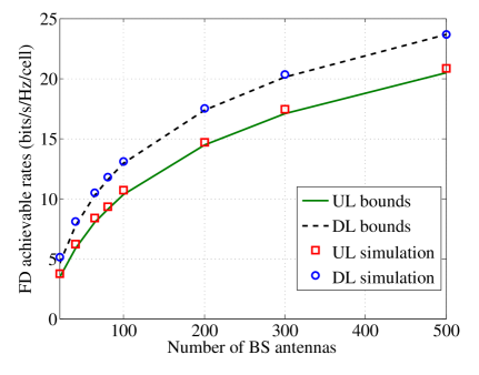
(a) With perfect CSI

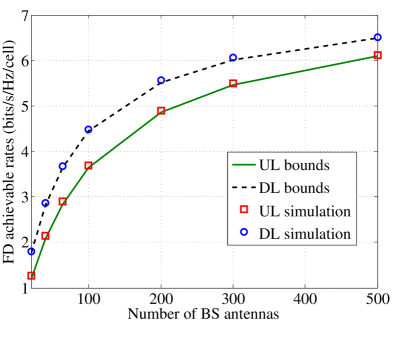
(b) With imperfect CSI

Figure 3: Comparisons between lower bounds in Proposition LABEL:prop1 and LABEL:prop2 and numerically evaluated values of the ergodic achievable rates (bits/s/Hz/cell) under both perfect and imperfect CSI assumptions, where $P_{tr}=P_{u}=10$ dB and $P_{d}=20$ dB.

We compute the spectral efficiency ratios between full-duplex and half-duplex by comparing the full-duplex rates given in (LABEL:homocsi) and (LABEL:homoerror) with the half-duplex achievable rates in (LABEL:ARHDP) and (LABEL:ARHDIP) which can be evaluated numerically. We consider the same setting as in Fig. 3 under both perfect and imperfect CSI assumptions. In Figure 4(a), in the case of perfect CSI, we can see that as $M$ increases, the up- and downlink spectral efficiency gain between full-duplex system versus TDD system will converge to 2 as we scale down the transmit power according to Theorem LABEL:prop3. The convergence rate is fast at the beginning, and becomes slower for large $M$. To reach the asymptotic $2\times$ gain, it will require remarkably large number of BS antennas. However, full-duplex spectral efficiency gains in both uplink and downlink are achievable for finite $M$. For example, when $M=64$, full-duplex achieves about 1.7$\times$ downlink gain and 1.3$\times$ uplink gain. We numerically show that even without scaling down the transmit power, similar full-duplex gains are achievable. Figure 4(b) shows the full-duplex over half-duplex spectral efficiency gains in the case of imperfect CSI. We observe that even with channel estimation error and pilot contamination, full-duplex uplink and downlink gains exist for finite $M$ with and without scaling down the transmit power.

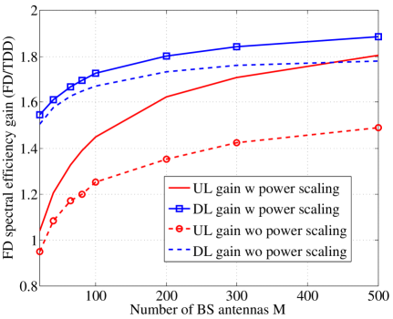
(a) With perfect CSI

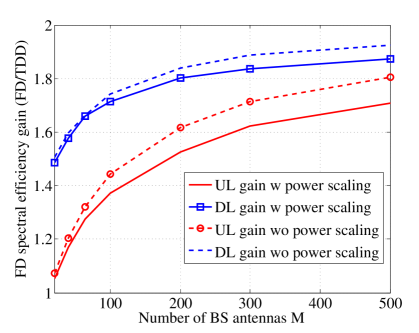
(b) With imperfect CSI

Figure 4: Spectral efficiency gains of using full-duplex for finite $M$ with and without power scaling.

We also investigate the spectral efficiency gain and antenna reduction tradeoff between full-duplex system and TDD system. The antenna reduction is the reduction of BS antennas due to full-duplex operation which can be characterized by the ratio between the number of BS antennas in TDD system ($M_{\rm{TDD}}$) and the number of BS antennas in FD system. The spectral efficiency gain and antenna reduction tradeoff is essentially the tradeoff between full-duplex multiplexing gain due to simultaneous transmission and reception and beamforming gain due to large $M$. In Fig. 5, we consider the same setting as in Fig. 3 under imperfect CSI assumption. We illustrate the spectral efficiency gain and antenna reduction tradeoff for both uplink and downlink with different $M_{\rm{TDD}}$ in the TDD system. Larger full-duplex antenna reduction can be achieved at the cost of reducing the spectral efficiency gain. In the regimes above the dashed arrows as shown in Fig. 5, full-duplex system achieves both spectral efficiency gain and antenna reduction over TDD system. We can see that full-duplex system can require an order of magnitude fewer BS antennas compared with TDD to obtain the same performance in some cases. In addition, as $M_{\rm{TDD}}$ increases, full-duplex system can achieve higher spectral efficiency gain and antenna reduction.

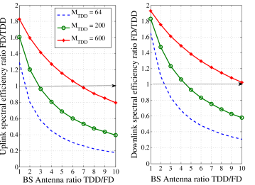
Figure 5: Spectral efficiency gain and antenna reduction tradeoff for various numbers of BS antennas employed in the TDD system under imperfect CSI assumption.

V Numerical Results

V-A A small cell scenario

Based on the state-of-art self-interference cancellation capability [1], the coverage of a full-duplex system is more likely to be within a small-cell communication ranges. Hence in this section, we present the numerical simulation in realistic small-cell network settings used in 3GPP [14] to evaluate the system performance. Twelve small cell BSs are uniformly and randomly distributed within a hexagonal region with a radius of $300$ meters All the small-cell BSs have full-duplex capability with multiple antennas. Each small-cell BS is associated with five single-antenna half-duplex uplink UEs and downlink UEs, respectively, which are uniformly and randomly dropped within a radius of 40 meters of the BS. The numerical results are shown for the case of imperfect CSI with channel estimation error. We consider an OFDM system and the coherence interval is $T=196$. The channel bandwidth is assumed as 20 MHz for both TDD and full-duplex systems. The large-scale fading models for BS-UE, BS-BS and UE-UE channels which include path loss and shadowing effect follow 3GPP model in [14]. The SI channel model is based on the existing experiment data [1], where the propagation loss of SI channel in a separate-antenna system includes path loss, isolation, cross-polarization and antenna directionality [3], and in a shared-antenna system includes isolation using a circulator. We assume the SI channel has a propagation loss of $40$ dB. We run hundreds of random drops of BSs and UEs in the simulation, and parameter details are given in Tabel I.

Parameter	Value
Full-duplex BS power	$24$ dBm
UE power	$23$ dBm
BS antenna gain	$5$ dBi
Number of BS antennas $M$	{$20,50,100,300,500$}
Thermal noise density	$-174$ dBm/Hz
Noise Figure	BS: 9 dB; UE: $5$ dB
Dynamic range $\kappa^{-1}$	{$50,60,70,80$} dB
Minimum distance constraints	BS-BS: $40$ m; BS-UE: $10$ m; UE-UE: $3$ m
Shadowing standard deviation	BS-UE: $10$ dB; BS-BS: $12$ dB; UE-UE: $6$ dB
Pathloss models for BS-UE, UE-UE,	Refer to [14]
and BS-BS channels
Fast fading channels	i.i.d. $\mathcal{CN}(0,1)$
Propagation loss of self-interference channels	$40$ dB [1]

TABLE I: Simulation parameters

The average full-duplex spectral efficiency gain is illustrated in Fig. 6 with varying numbers of BS antennas, where the dynamic range parameter $\kappa$ is $-60$ dB. We verify that the full-duplex gains in realistic network scenarios exist for a range of finite number of BS antennas and the gains will scale with BS antennas. Fig 7 depicts the average spectral efficiency gain of the full-duplex system for different dynamic range parameters $\kappa$ when $M=100$, which demonstrates the impact of imperfect SI cancellation. Since all users are half-duplex, the downlink gains are not affected by $\kappa$. However, since all the BSs are full-duplex, the uplink gains are severely affected by the dynamic range values especially when the dynamic range value is low. We can see that larger dynamic range $\kappa^{-1}$, (i.e., smaller $\kappa$) will result in less residual SI, thus increasing the uplink gain. Once the dynamic range $\kappa^{-1}$ exceeds certain threshold, there is not much impact of the residual SI on the uplink performance.

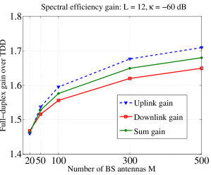
Figure 6: Average full-duplex spectral efficiency gain with BS antenna arrays when $L=12$ and $\kappa=-60$.

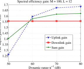
Figure 7: Average full-duplex spectral efficiency gain with different dynamic ranges when $M=100$ and $L=12$.

VI Conclusion

In this paper, we have investigated the multi-cell MU-MIMO full-duplex networks where single-antenna full-duplex and half-duplex UEs are served by the full-duplex BSs with multiple antennas. Using low complexity linear receivers and precoders, the ergodic achievable rates of uplink and downlink are characterized for the full-duplex system. Several practical constraints are modeled in the analysis such as imperfect full-duplex radio chains, channel estimation error, pilot overhead and pilot contamination. The large scale system performance is analyzed when each BS has a large antenna array. When the number of BS antennas grows infinitely large, the 2$\times$ asymptotic full-duplex spectral efficiency gain can be achieved over the TDD system with perfect CSI. When channel estimation error and channel training overhead are considered, the 2$\times$ asymptotic full-duplex spectral efficiency gain is achieved when serving only full-duplex UEs. Furthermore, we show by numerical simulation that full-duplex system can achieve both spectral efficiency gain and antenna reduction as the full-duplex system can require one order of magnitude fewer antennas than TDD to achieve the same or better performance in certain cases.

-A Proof of Proposition LABEL:prop1

Based on Jensen’s inequality and the convexity of $\mathrm{log}_{2}\left(1+x^{-1}\right)$, we have $\mathbb{E}\left[\mathrm{log}_{2}\left(1+x^{-1}\right)\right]\geq\mathrm{log}_{2}\left(1+\mathbb{E}^{-1}(x)\right)$. Hence we can lower bound the ergodic achievable rate of the $n$-th uplink UE in the $j$-th cell in (LABEL:ul:lb1) as

$$\begin{aligned} &\tilde{R}^{fd,p}_{u,jn}\geq R^{fd,p}_{u,jn}\triangleq\mathrm{log}_{2}\Bigg{(}1+\\ &\mathbb{E}^{-1}\left[\frac{P_{u}\sum_{(l,m)\neq(j,n)}|\bm{g}^{H}_{u,jjn}\bm{g}_{u,jlm}|^{2}+I_{bs-bs}+\left\lVert\bm{g}_{u,jjn}\right\rVert^{2}(\sigma^{2}+\kappa P_{d}\beta_{b,jj})}{P_{u}\left\lVert\bm{g}_{u,jjn}\right\rVert^{4}}\right]\Bigg{)}\\ &=\mathrm{log}_{2}\left(1+\mathbb{E}^{-1}\left[\frac{P_{u}\sum_{(l,m)\neq(j,n)}|\tilde{g}_{u,jlm}|^{2}+\sum_{l\neq j}\sum_{k\in\mathcal{K}_{d}}\frac{P_{d}}{K_{d}\gamma_{l}}|\tilde{v}_{jlk}|^{2}+\sigma^{2}+\kappa P_{d}\beta_{b,jj}}{P_{u}\left\lVert\bm{g}_{u,jjn}\right\rVert^{2}}\right]\right),\end{aligned}$$ (41)

where $\tilde{g}_{u,jlm}\triangleq\frac{\bm{g}^{H}_{u,jjn}\bm{g}_{u,jlm}}{\left\lVert\bm{g}_{u,jjn}\right\rVert}$, $\tilde{v}_{jlk}\triangleq\frac{\bm{g}^{H}_{u,jjn}\bm{V}_{jl}\bm{g}^{*}_{d,llk}}{\left\lVert\bm{g}_{u,jjn}\right\rVert}$. Conditioned on $\bm{g}_{u,jjn}$, $\tilde{g}_{u,jlm}\sim\mathcal{CN}(0,\beta_{u,jlm})$ and $\tilde{v}_{jlk}\sim\mathcal{CN}(0,M\beta_{b,jl}\beta_{d,llk})$ are independent of $\bm{g}_{u,jjn}$. Thus we have

$$\begin{aligned} &\mathbb{E}\left[\frac{P_{u}\sum_{(l,m)\neq(j,n)}|\tilde{g}_{u,jlm}|^{2}+\sum_{l\neq j}\sum_{k\in\mathcal{K}_{d}}\frac{P_{d}}{K_{d}\gamma_{l}}|\tilde{v}_{jlk}|^{2}+\sigma^{2}+\kappa P_{d}\beta_{b,jj}}{P_{u}\left\lVert\bm{g}_{u,jjn}\right\rVert^{2}}\right]\\ &=\left(\sum_{(l,m)\neq(j,n)}P_{u}\mathbb{E}[|\tilde{g}_{u,jlm}|^{2}]+\sum_{l\neq j}\sum_{k\in\mathcal{K}_{d}}\frac{P_{d}}{K_{d}\gamma_{l}}\mathbb{E}[|\tilde{v}_{jlk}|^{2}]+\sigma^{2}+\kappa P_{d}\beta_{b,jj}\right)\mathbb{E}\left[\frac{1}{P_{u}\left\lVert\bm{g}_{u,jjn}\right\rVert^{2}}\right].\end{aligned}$$ (42)

From Lemma 2.10 in [29], for a central Wishart matrix $\bm{W}\sim\mathcal{W}_{m}(n,\bm{I})$ with $n\geq m$, we have $\mathbb{E}[\mathsf{tr}\{\bm{W}^{-1}\}]=\frac{m}{n-m}$ for $n>m$. Hence

$$\begin{aligned} \mathbb{E}\left[\frac{1}{P_{u}\left\lVert\bm{g}_{u,jjn}\right\rVert^{2}}\right]=\frac{1}{(M-1)P_{u}\beta_{u,jjn}}~{}\text{for}~{}M\geq 2.\end{aligned}$$ (43)

Combing (41), (42) and (43), we can obtain the uplink achievable rate in (LABEL:eq:prop1).

To derive the lower bound on the downlink achievable rate, we need to evoke the Lemma 2.10 in [29] again where $\mathbb{E}[\mathsf{tr}\{\bm{W}^{-2}\}]=\frac{mn}{(n-m)^{3}-(n-m)}$ for $n>m+1$. Thus we have

$$\begin{aligned} \mathbb{E}\left[\frac{1}{\left\lVert\bm{g}_{d,llk}\right\rVert^{4}}\right]=\frac{1}{(M-1)(M-2)\beta_{d,llk}^{2}}~{}\text{for}~{}M\geq 3.\end{aligned}$$ (44)

Following the same approach used in the derivation of uplink rate, we can obtain the achievable rate of each downlink user given in proposition LABEL:prop1. The details are omitted to avoid redundancy.

-B Proof of Proposition LABEL:prop2

Similar to the proof of Proposition LABEL:prop1, applying Jensen’s inequality, we can lower bound the ergodic achievable rate of the $n$-th uplink user in the $j$-th cell in (LABEL:ulim:lb1) as

$$\begin{aligned} &\tilde{R}^{fd,ip}_{u,jn}\geq R^{fd,ip}_{u,jn}\triangleq\mathrm{log}_{2}\Bigg{(}1+\\ &\mathbb{E}^{-1}\left[\frac{P_{u}\lvert\tilde{\epsilon}_{jjn}\rvert^{2}+P_{u}\sum_{(l,m)\neq(j,n)}|\tilde{\tilde{g}}_{u,jlm}|^{2}+\sum_{l\neq j}\sum_{k\in\mathcal{K}_{d}}\frac{P_{d}}{K_{d}\gamma_{l}}|\tilde{\tilde{v}}_{jlk}|^{2}+\sigma^{2}+\kappa P_{d}\beta_{b,jj}}{P_{u}\left\lVert\hat{\bm{g}}_{u,jjn}\right\rVert^{2}}\right]\Bigg{)}\end{aligned}$$ (45)

where $\tilde{\epsilon}_{jjn}\triangleq\frac{\hat{\bm{g}}^{H}_{u,jjn}\bm{\epsilon}_{u,jjn}}{\left\lVert\hat{\bm{g}}_{u,jjn}\right\rVert}$, $\tilde{\tilde{g}}_{u,jlm}\triangleq\frac{\hat{\bm{g}}^{H}_{u,jjn}\bm{g}_{u,jlm}}{\left\lVert\hat{\bm{g}}_{u,jjn}\right\rVert}$, $\tilde{\tilde{v}}_{jlk}\triangleq\frac{\hat{\bm{g}}^{H}_{u,jjn}\bm{V}_{jl}\hat{\bm{g}}^{*}_{d,llk}}{\left\lVert\bm{g}_{u,jjn}\right\rVert}$. Conditioned on $\hat{\bm{g}}_{u,jjn}$, $\tilde{\epsilon}_{jjn}\sim\mathcal{CN}\left(0,\frac{\beta_{u,jjk}\left(\sigma^{2}+P_{tr}\sum_{l\neq j}\beta_{u,jlk}\right)}{\lambda_{u,jk}}\right)$, $\tilde{\tilde{v}}_{jlk}\sim\mathcal{CN}\left(0,M\beta_{b,jl}\frac{P_{tr}\beta^{2}_{d,llk}}{\lambda_{d,lk}}\right)$ and $\tilde{\tilde{g}}_{u,jlm}\sim(0,\mathrm{var}(\tilde{\tilde{g}}_{u,jlm}))$ are independent of $\hat{\bm{g}}_{u,jjn}$. Using (LABEL:eq:mmse), we have

$$\begin{aligned} \tilde{\tilde{g}}_{u,jlm}=\frac{P_{tr}\beta_{u,jjn}}{\lambda_{u,jn}}\left(\sum_{l_{1}=1}^{L}\bm{g}^{H}_{u,jl_{1}n}+\frac{\bm{n}^{H}_{jn}}{\sqrt{P_{tr}}}\right)\frac{\bm{g}_{u,jlm}}{\left\lVert\hat{\bm{g}}_{u,jjn}\right\rVert}.\end{aligned}$$ (46)

Evoking Lemma 2.9 in [29], where for a central Wishart matrix $\bm{W}\sim\mathcal{W}_{m}(n,\bm{I})$ with $n\geq m$, $\mathbb{E}[\mathsf{tr}\{\bm{W}^{2}\}]=mn(m+n)$, we can calculate the variance of $\tilde{\tilde{g}}_{u,jlm}$ as

$$\begin{aligned} \mathbb{E}[\lvert\tilde{\tilde{g}}_{u,jlm}\rvert^{2}]=\begin{cases}\frac{P_{tr}}{\lambda_{u,jn}}\left[(M+1)\beta^{2}_{u,jln}+\sum_{l_{1}\neq l}\beta_{u,jl_{1}n}\beta_{u,jln}+\frac{\beta_{u,jln}\sigma^{2}}{P_{tr}}\right]&~{}~{}m=n,l\neq j\\ \beta_{u,jlm}&~{}~{}m\neq n.\end{cases}\end{aligned}$$ (47)

Now we can rewrite the expectation in (45) as

$$\begin{aligned} &\mathbb{E}\left[\frac{P_{u}\lvert\tilde{\epsilon}_{jjn}\rvert^{2}+P_{u}\sum_{(l,m)\neq(j,n)}|\tilde{\tilde{g}}_{u,jlm}|^{2}+\sum_{l\neq j}\sum_{k\in\mathcal{K}_{d}}\frac{P_{d}}{K_{d}\gamma_{l}}|\tilde{\tilde{v}}_{jlk}|^{2}+\sigma^{2}+\kappa P_{d}\beta_{b,jj}}{P_{u}\left\lVert\hat{\bm{g}}_{u,jjn}\right\rVert^{2}}\right]\\ &=\left(P_{u}\mathbb{E}[|\tilde{\epsilon}_{jjn}|^{2}]+P_{u}\sum_{\mathclap{(l,m)\neq(j,n)}}\mathbb{E}[|\tilde{\tilde{g}}_{u,jlm}|^{2}]+\sum_{l\neq j}\sum_{k\in\mathcal{K}_{d}}\frac{P_{d}}{K_{d}\gamma_{l}}\mathbb{E}[|\tilde{\tilde{v}}_{jlk}|^{2}]+\sigma^{2}+\kappa P_{d}\beta_{b,jj}\right)\mathbb{E}\left[\frac{1}{P_{u}\left\lVert\hat{\bm{g}}_{u,jjn}\right\rVert^{2}}\right].\end{aligned}$$ (48)

Combing (45), (47) and (48), we can obtain the uplink achievable rate in (LABEL:eq:prop2).

For the downlink achievable rate in (LABEL:dlim:lb1), we first compute $\mathbb{E}\left[\bm{g}^{T}_{d,llk}\hat{\bm{g}}^{*}_{d,llk}\right]$. Let $\mu=\bm{g}^{T}_{d,llk}\hat{\bm{g}}^{*}_{d,llk}$, since $\bm{g}_{d,llk}=\hat{\bm{g}}_{d,llk}+\bm{\epsilon}_{d,llk}$ and $\hat{\bm{g}}_{d,llk}$ is independently of $\bm{\epsilon}_{d,llk}$, we have

$$\begin{aligned} \mathbb{E}[\mu]&=\mathbb{E}\left[(\hat{\bm{g}}^{T}_{d,llk}+\bm{\epsilon}^{T}_{d,llk})\hat{\bm{g}}^{*}_{d,llk}\right]\\ &=\mathbb{E}\left[\left\lVert\hat{\bm{g}}_{d,llk}\right\rVert^{2}\right]=\frac{MP_{tr}\beta^{2}_{d,llk}}{\lambda_{d,lk}}.\end{aligned}$$ (49)

Again invoking Lemma 2.9 in [29], we have

$$\begin{aligned} \mathbb{E}\left[\mu^{2}\right]&=\mathbb{E}\left[\left\lVert\hat{\bm{g}}_{d,llk}\right\rVert^{4}\right]+\mathbb{E}\left[\bm{\epsilon}^{T}_{d,llk}\hat{\bm{g}}^{*}_{d,llk}\hat{\bm{g}}^{T}_{d,llk}\bm{\epsilon}^{*}_{d,llk}\right]\\ &=\frac{M(M+1)P^{2}_{tr}\beta^{4}_{d,llk}+MP_{tr}\beta^{3}_{d,llk}(\sigma^{2}+P_{tr}\sum_{j\neq l}\beta_{d,ljk})}{\lambda_{d,lk}^{2}}.\end{aligned}$$ (50)

Since $\mathsf{var}\left[\bm{g}^{T}_{d,llk}\hat{\bm{g}}^{*}_{d,llk}\right]\triangleq\mathsf{var}(\mu)=\mathbb{E}(\mu^{2})-\mathbb{E}^{2}(\mu)$, we can obtain that

$$\begin{aligned} \mathsf{var}(\mu)&=\frac{MP_{tr}\beta^{3}_{d,llk}}{\lambda_{d,lk}}.\end{aligned}$$ (51)

Next, we compute $\mathbb{E}\left[\lvert\bm{g}^{T}_{d,jlk}\hat{\bm{g}}^{*}_{d,jji}\rvert^{2}\right]$ as

$$\begin{aligned} \mathbb{E}\left[\lvert\bm{g}^{T}_{d,jlk}\hat{\bm{g}}^{*}_{d,jji}\rvert^{2}\right]=\begin{cases}\frac{MP^{2}_{tr}\beta^{2}_{d,jjk}}{\lambda^{2}_{d,jk}}\!\!\left[(M+1)\beta^{2}_{d,jlk}+\sum_{l_{1}\neq l}\beta_{d,jl_{1}k}\beta_{d,jlk}+\frac{\beta_{d,jlk}\sigma^{2}}{P_{tr}}\right]&~{}~{}i=k,j\neq l\\ \frac{MP_{tr}\beta^{2}_{d,jji}\beta_{d,jlk}}{\lambda_{d,ji}}&~{}~{}i\neq k.\end{cases}\end{aligned}$$ (52)

The rest terms in (LABEL:dlim:lb1) can be calculated easily, and thus the details are omitted. Combing all the results above, we can obtain downlink achievable rate given in proposition LABEL:prop2.

References

- [1] A. Sabharwal, P. Schniter, D. Guo, D. Bliss, S. Rangarajan, and R. Wichman, “In-band full-duplex wireless: Challenges and opportunities,” Selected Areas in Communications, IEEE Journal on, vol. 32, no. 9, pp. 1637–1652, Sept 2014.
- [2] M. Duarte, A. Sabharwal, V. Aggarwal, R. Jana, K. Ramakrishnan, C. Rice, and N. Shankaranarayanan, “Design and characterization of a full-duplex multiantenna system for WiFi networks,” Vehicular Technology, IEEE Transactions on, vol. 63, no. 3, pp. 1160–1177, 2014.
- [3] E. Everett, A. Sahai, and A. Sabharwal, “Passive self-interference suppression for full-duplex infrastructure nodes,” Wireless Communications, IEEE Transactions on, vol. 13, no. 2, pp. 680–694, February 2014.
- [4] D. Bharadia, E. McMilin, and S. Katti, “Full duplex radios,” in Proceedings of the ACM SIGCOMM 2013 Conference on SIGCOMM, ser. SIGCOMM ’13. New York, NY, USA: ACM, 2013, pp. 375–386.
- [5] E. Aryafar, M. A. Khojastepour, K. Sundaresan, S. Rangarajan, and M. Chiang, “MIDU: enabling MIMO full duplex,” in Proceedings of the 18th annual international conference on Mobile computing and networking. ACM, 2012, pp. 257–268.
- [6] D. Kim, H. Lee, and D. Hong, “A survey of in-band full-duplex transmission: From the perspective of PHY and MAC layers,” IEEE Communications Surveys Tutorials, vol. 17, no. 4, pp. 2017–2046, Fourthquarter 2015.
- [7] E. Hossain and M. Hasan, “5G cellular: Key enabling technologies and research challenges,” 2015. [Online]. Available: http://arxiv.org/abs/1503.00674
- [8] C. Shepard, H. Yu, and L. Zhong, “Argosv2: A flexible many-antenna research platform,” in Proceedings of the 19th Annual International Conference on Mobile Computing & Networking, ser. MobiCom ’13. New York, NY, USA: ACM, 2013, pp. 163–166.
- [9] E. G. Larsson, O. Edfors, F. Tufvesson, and T. L. Marzetta, “Massive MIMO for next generation wireless systems,” IEEE Communications Magazine, vol. 52, no. 2, pp. 186–195, 2014.
- [10] F. Rusek, D. Persson, B. K. Lau, E. G. Larsson, T. L. Marzetta, O. Edfors, and F. Tufvesson, “Scaling up MIMO: Opportunities and challenges with very large arrays,” Signal Processing Magazine, IEEE, vol. 30, no. 1, pp. 40–60, 2013.
- [11] T. Marzetta, “Noncooperative cellular wireless with unlimited numbers of base station antennas,” Wireless Communications, IEEE Transactions on, vol. 9, no. 11, pp. 3590–3600, November 2010.
- [12] H. Q. Ngo, E. Larsson, and T. Marzetta, “Energy and spectral efficiency of very large multiuser MIMO systems,” Communications, IEEE Transactions on, vol. 61, no. 4, pp. 1436–1449, April 2013.
- [13] http://www.3gpp.org/news-events/3gpp-news/1628-rel13.
- [14] 3GPP. Further enhancements to LTE time division duplex (TDD) for downlink-uplink (DL-UL) interference management and traffic adaptation,TR 36.828, v.11.0.0. [Online]. Available: www.3gpp.org
- [15] A. Sahai, S. Diggavi, and A. Sabharwal, “On degrees-of-freedom of full-duplex uplink/downlink channel,” in Information Theory Workshop (ITW), 2013 IEEE, Sept 2013, pp. 1–5.
- [16] J. Bai, S. Diggavi, and A. Sabharwal, “On degrees-of-freedom of multi-user MIMO full-duplex network,” in Information Theory (ISIT), 2015 IEEE International Symposium on, June 2015, pp. 864–868.
- [17] S. Jeon, S. H. Chae, and S. H. Lim, “Degrees of freedom of full-duplex multiantenna cellular networks,” Jan 2015. [Online]. Available: http://arxiv.org/abs/1501.02889
- [18] C. Karakus and S. Diggavi, “Opportunistic scheduling for full-duplex uplink-downlink networks,” in Information Theory (ISIT), 2015 IEEE International Symposium on, June 2015, pp. 1019–1023.
- [19] W. Ouyang, J. Bai, and A. Sabharwal, “Leveraging one-hop information in massive MIMO full-duplex wireless systems,” Submitted to IEEE/ACM Transactions on Networking, Sep 2015. [Online]. Available: http://arxiv.org/abs/1509.00539
- [20] J. Bai and A. Sabharwal, “Distributed full-duplex via wireless side-channels: Bounds and protocols,” Wireless Communications, IEEE Transactions on, vol. 12, no. 8, pp. 4162–4173, 2013.
- [21] S. Goyal, P. Liu, S. Hua, and S. Panwar, “Analyzing a full-duplex cellular system,” in Information Sciences and Systems (CISS), 2013 47th Annual Conference on, 2013, pp. 1–6.
- [22] Y. S. Choi and H. Shirani-Mehr, “Simultaneous transmission and reception: Algorithm, design and system level performance,” IEEE Transactions on Wireless Communications, vol. 12, no. 12, pp. 5992–6010, December 2013.
- [23] M. Amir Khojastepour, K. Sundaresan, S. Rangarajan, and M. Farajzadeh-Tehrani, “Scaling wireless full-duplex in multi-cell networks,” in Computer Communications (INFOCOM), 2015 IEEE Conference on, April 2015, pp. 1751–1759.
- [24] B. Day, A. Margetts, D. Bliss, and P. Schniter, “Full-duplex bidirectional MIMO: Achievable rates under limited dynamic range,” Signal Processing, IEEE Transactions on, vol. 60, no. 7, pp. 3702–3713, July 2012.
- [25] M. Vehkapera, T. Riihonen, and R. Wichman, “Asymptotic analysis of full-duplex bidirectional MIMO link with transmitter noise,” in Personal Indoor and Mobile Radio Communications (PIMRC), 2013 IEEE 24th International Symposium on, Sept 2013, pp. 1265–1270.
- [26] J. Hoydis, S. ten Brink, and M. Debbah, “Massive MIMO in the UL/DL of cellular networks: How many antennas do we need?” Selected Areas in Communications, IEEE Journal on, vol. 31, no. 2, pp. 160–171, February 2013.
- [27] J. Jose, A. Ashikhmin, T. L. Marzetta, and S. Vishwanath, “Pilot contamination and precoding in multi-cell tdd systems,” IEEE Transactions on Wireless Communications, vol. 10, no. 8, pp. 2640–2651, 2011.
- [28] H. Cramér, random variables and probability distributions. Cambridge University Press, 1970.
- [29] A. M. Tulino and S. Verdú, Random matrix theory and wireless communications. Now Publishers Inc, 2004, vol. 1.