1.0
Inscribed Matter Communication: Part I
Abstract
We provide a fundamental treatment of the molecular communication channel wherein “inscribed matter” is transmitted across a spatial gap to provide reliable signaling between a sender and receiver. Inscribed matter is defined as an ensemble of “tokens” (biotic/abiotic objects) and is inspired, at least partially, by biological systems where groups of individually constructed discrete particles ranging from molecules to viruses and organisms are released by a source and travel to a target – for example, morphogens or semiochemicals diffuse from one cell, tissue or organism to another. For identical tokens that are neither lost nor modified, we consider messages encoded using three candidate communication schemes: a) token timing (timed release), b) token payload (composition), and c) token timing plus payload. We provide capacity bounds for each scheme and discuss their relative utility. We find that under not unreasonable assumptions, megabit per second rates could be supported at femtoWatt transmitter powers. Also, since quantities such as token concentration or token-counting are derivatives of token arrival timing, token timing undergirds all molecular communication techniques. Thus, our modeling and results about the physics of efficient token-based information transfer can inform investigations of diverse theoretical and practical problems in engineering and biology. This work, Part I, focuses on the information theoretic bounds on capacity. Part-II develops some of the mathematical and information-theoretic machinery that support the bounds presented here.
I Introduction
Scale-appropriate signaling methods become important as systems shrink to the nanoscale. For systems with feature sizes of microns and smaller, electromagnetic and acoustic communication become increasingly inefficient because energy coupling from the transmitter to the medium and from the medium to the receiver becomes difficult at usable frequencies. Biological systems, with the benefit of lengthy evolutionary experimentation, seem to have arrived at a ubiquitous solution to this signaling problem at small and not so small scales: use of “inscribed matter” (an ensemble of discrete particles) which travels through some material bearing a message from one entity to another. Broad classes of such particles include
-
•
Molecules such as electronically activated species, ions, chemicals, biopolymers, and macromolecular complexes.
-
•
Membrane-bound structures such as intra- and extracellular vesicles (for instance, exosomes, microvesicles, apoptotic bodies, ectosomes, endosomes, lysosomes, autophagosomes, and vacuoles) and intracellular organelles (for instance, nuclei, mitochondria, and chloroplasts).
-
•
Cells such as stem cells, tumor cells, and hematocytes.
-
•
Acellular, unicellular and multicellular life forms (organisms for brevity) such as viruses, viroids, phages, plasmids, bacteria, archaea, fungi, protists, plants, and animals.
-
•
Objects such as matter in the natural world (for instance pollen grains, seeds, and proteinaceous aggregates such as prions); and human artifacts (for example, Voyager Golden Records).
Studies of engineered nano-scale communication systems have focused on the encoding, transmission, and decoding of information using patterns of one category of discrete particles, namely molecules. A large portion of this work in “molecular communication” has considered time-varying concentration profiles of molecules as the fundamental signal measurement [1, 2, 3, 4, 5, 6, 7]. However, concentration is a collective property of the process and masks the underlying physics of molecule release by the sender and capture by the receiver. This begs the questions of truly fundamental limits for communication using ensembles of molecules in particular, discrete particles more broadly, and what we term “tokens” in general.
This paper is organized as follows:
First, we discuss communication using inscribed matter from biological and engineering perspectives. We illustrate how scenarios spanning a wide range of spatial and temporal scales and from seemingly disparate disciplines can be understood within a unified framework: the token timing and/or token payload channel, a communication scheme wherein information is carried from sender to receiver by tokens via their timed release, their composition, or both.We will assume tokens always (eventually) arrive, and are removed from circulation upon first seizure by the receiver. This abstraction encompasses not only token timing but also the token concentration and token counting models prevalent in the molecular communication literature [1, 2, 3, 4, 5, 6, 7, 8, 9].
Next, we describe the token timing channel wherein information is encoded only in the release time of identical tokens as opposed to inscribed onto tokens (tokens with payloads) or in the number of tokens released (token counting). Though seemingly limited, this pure timing model supplies the mathematical machinery to precisely consider both token payload and token counting communication schemes. To this end, we provide a mathematical formulation of token timing channel: identical tokens emitted with independent stochastic (but asymptotically assured, one-time) arrivals. We formalize the signaling model so that the typical energy-dependent asymptotic sequential channel use coding results based on mutual information between input and output can be applied [10, (chapt 8 & 10)]. We then show how these results can be applied to token counting and tokens with payloads. We focus on molecular tokens – particularly DNA and protein sequences since their energy requirements (and information content) are well-understood – and show that information transfer using inscribed matter can be extremely efficient. We find that megabit per second rates could be supported theoretically with on the order of femtoWatts of transmitter power.
Finally, we explore how our studies and the attendant insights could aid biological understanding of and inform engineering approaches to inscribed matter communication.
II Inscribed Matter
II-A Communication using discrete particles: a natural world perspective
Networks of intercommunicating biological entities occur at whatever level one cares to consider: (macro)molecules, cells, tissues, organisms, populations, microbiomes, ecosystems, and so on. An ancient yet still widespread method for one entity to convey a message to another is via inscribed matter. The typical scenario is as follows: information-bearing discrete particles are released by a source, travel through a material, and are captured by a target where they are interpreted. The following examples illustrate the diversity and complexity of such inscribed matter communication (the particles are italicized).
-
•
Electrons from an electron donor flow through an electron transport chain to an electron acceptor where the electrochemical gradient is used convert mechanical work into chemical energy as part of a cellular process such as photosynthesis or respiration. In microbial communities, electrons are transferred from one individual to another through bacterial nanowires (electrically conductive appendages), bacterial cables (thousands of individuals lined up end-to-end with electron donors located in the deeper regions of marine sediment and electron acceptors positioned in its upper layers where oxygen is more abundant), and biofilms (community members embedded in a self-produced three-dimensional matrix of extrapolymeric substances) [11].
-
•
Free radicals produced from molecules in the nucleoplasm by the direct or indirect action of ionizing radiation diffuse to the genome where they alter/damage nucleotide bases and sugars.
-
•
messenger RNA (mRNA) molecules transcribed from a eukaryotic genome in a nucleus migrate to ribosomes in the cytoplasm where they are translated into proteins.
-
•
Acetylcholine (ACh) molecules released by a vertebrate motor neuron diffuse across the synapse to nicotinic ACh receptors on the plasma membrane of the muscle fiber where binding triggers muscular contraction.
-
•
Homing endonuclease (HE) containing inteins self-excised from bacterial, archaeal, eukaryotic or viral host proteins home to a target site in the genome of the same or different organism where the genetic parasitic element reinserts itself into the intein-free allele of the host gene (horizontal dissemination); inteins without a functioning HE are mainly transferred vertically but may move horizontally along with the host gene.
-
•
Ions, molecules, organelles, bacteria and viruses present in one cell travel through a thin membrane channel (tunneling nanotube) to the physically connected cell where they elicit a response.
-
•
Semiochemicals (chemical substances or mixtures of volatile molecules) emitted by one individual travel to another of the same (pheromones) or different species (allelochemicals) where they elicit a response – allomones benefit only the sender, kairomone benefit only the receiver, and synomones benefit both.
-
•
Extracellular vesicles secreted by all living cells – including bacteria, archaea and eukaryotes – and harboring specific cargo materials (for instance, proteins, nucleic acids, lipids, metabolites, antigens, and viruses) traverse the extracellular space or body fluids (for instance, blood and urine) to a local or distal recipient cell where they transfer their bioactive contents.
-
•
Cargo-bearing molecular motors shuttle along a track system of cytoskeletal filaments to another point in the cell compartment where their freight such as vesicles containing molecules and tubes is unloaded.
-
•
Single and clusters of metastatic cells that have escaped from a primary tumor circulate through the blood or lymph to a secondary organ site where, after extravasation, they can seed a new tumor.
-
•
Organic particles such as microorganisms, fungal spores, small insects, and pollen grains associated with a macroorganism, geological site or geographic location relocate to another host or region where they influence the local biochemistry, geochemistry and climate [12]– long distance transport (including movement within and between continents and oceans) can occur via the same meteorological phenomena and processes, such as jetstreams and hurricanes, that translocate non-biological particles such as sea salt and dust.
-
•
Crustal material ejected by a Solar System body travels to another body where if it carries microbial spores or building blocks such as amino acids, nucleobases and lipid-like molecules has the potential to seed life. Ejecta (potentially carrying microbial spores) travel from Ceres (the largest object in the asteroid belt which lies between the orbits of Mars and Jupiter) to terrestrial planets in the solar system (Earth, Mars or Venus) [13]; the presence of water on Ceres [14] suggests the dwarf planet’s potential as a home for extraterrestrial life.
Irrespective of the precise nature of the components of the inscribed matter communication system – the discrete particles (information carriers), source (sender), spatial gap (transmission medium), and target (receiver) – two fundamental questions are “How reliable is communication?,” and “How is useful information conveyed given constraints on resources?.” Here, we investigate token timing (discrete particle release and capture times) and token payload (energy required to manufacture discrete particles, to assemble symbolic strings from a set of building blocks – we do not consider the energy required for de novo synthesis of the building blocks). And although not explicitly stated, please note that our energy model could also include token sequestration, token ejection, and token transport, the active movement of discrete particles (the energetics of translocating vesicles by a molecular motor system which converts chemical or other form of energy into mechanical energy). The only requirement is that the energy cost per token is independent of the information carried.
In the token timing channel model we will elaborate later on, tokens are neither lost nor modified: the number and makeup of the tokens emitted by the source is the same as the ones arriving at the target, all that differs are their times of emission and their times of arrival. While accommodating tokens that are delayed temporarily, our mathematical model does not directly consider tokens that are detained permanently, removed entirely, never arrive, or are changed en route. In the natural world, discrete particles often interact with the material through which they travel resulting in their immurement and ultimate removal or detention and eventual discharge. Examples include:
-
•
Free radicals produced by radiolysis may react chemically with neighboring materials.
-
•
mRNAs may be modified post-transcriptionally.
-
•
ACh can be degraded by the enzyme acetylcholine esterase present in synapses.
-
•
The random path of a semiochemical diffusing through air, soil or water may result in a trajectory that leads away from the destined individual.
-
•
Circulating tumor cells may be destroyed by the immune system.
-
•
Microscopic particles may be immobilized within mucus – the polymer-based hydrogel covering the inner linings of the body – depending on the density of the mucin network and environmental factors such as pH and ionic strength.
-
•
Bacteria, particularly plant pathogens, present in the atmosphere can nucleate the formation of ice in clouds resulting in snow, rain and hail [12].
Nonetheless, our model does provide an organizing principle for all forms of molecular communications since these sorts of impediments – token loss or corruption – can only decrease the capacity of the system we analyze. Furthermore, the analysis is “compartmental” in the sense that token corruption and loss can be treated separately without invalidating the fundamental “outer bound” results.
II-B Communication using physical objects: an engineering perspective
Inscribed matter can often be the most energy-efficient means of communication when delay can be tolerated. In fact, a once popular communication networks textbook [15] contains the passage:
Never underestimate the bandwidth of a station wagon full of tapes hurtling down the highway.
– A.S. Tanenbaum, Computer Networks, 4th ed., p. 91
This somewhat tongue-in-cheek “folklore” should come as no surprise. From early antiquity, private persons, governments, the military, press agencies, stockbrokers and others have used carrier pigeons to convey messages. Today, “sneakernets” [16] have been proposed as a low-latency high-fidelity network architecture for quantum computing across global distances: ships carry error-corrected quantum memories installed in cargo containers [17].
Previous work on mobile wireless communication found that network capacity could be increased if delay-tolerant traffic was queued until the receiver and sender were close to one another – perhaps close enough to exchange physical storage media [18, 19, 20, 21, 22, 23, 24, 25, 26, 27, 28, 29, 30, 31]. This recognition prompted a careful consideration of the energetics involved in delivery of physical messages, and a series of papers [32, 33, 34] revealed the surprising results that inscribed matter can be many orders of magnitude more efficient than radiative methods even with moderate delay constraints and over a variety of size scales. In fact, [34] showed that over interstellar distances (10k light years), inscribed matter could be on the order of times more energy-efficient than radiated messages, suggesting that evidence of extraterrestrial civilizations would more likely come from artifacts than from radio messages if energy requirements are a proxy for engineering difficulty [35].
At the other end of the size scale there has been increasing interest in biologically-inspired inscribed matter communication at the nano/microscale [36] where the information carrier ranges from timed release of identical signaling agents to specially constructed information carriers [37, 38, 1, 2, 3, 39, 4, 5, 6, 7, 40]. Although this field of molecular communication is in its infancy with seemingly futuristic application plans currently out of reach (for instance, in vivo biological signaling, surgical/medicinal/environmental microbot swarms, or process-on-a-chip), the theoretical potential rates and energy efficiencies, especially through media unfriendly to radiation, are sufficiently large [41] to warrant careful theoretical and practical consideration.
From an engineering perspective, the basic idea of inscribed matter communication is very simple (FIGURE 1). Information is coded in the structure of the signaling agent and/or its release time at the sender. These agents traverse some spatial gap to the receiver where they are captured and the information decoded. There are, of course, many details and variations on the theme. As explicitly mentioned for biological systems, the signaling agents (or tokens as we call them) could be identical, implying that timing (which includes time-varying concentration) is the only information carrier, or tokens could themselves carry data payloads (in addition to, or in lieu of timing). However, unlike the award-winning paper “Bits Through Queues” by Anantharam and Verdú [42] and later by Sundaresan and Verdú [43, 44], we do not know which arrival times correspond to which emission times.
The “gap” (channel) could be a medium through which tokens diffuse stochastically, or some form of active transport might be employed. In addition, tokens could be deliberately “eaten” by gettering agents injected by the sender, channel or receiver. Similarly, tokens could be corrupted during passage through the channel or might simply get “lost” and never reach the receiver [39, 9].
Furthermore, the reception process itself could be noisy. If we sought to mimic biological systems, a typical receptor structure is stereochemically matched to a particular signaling molecule (token) and the kinetics of the ligand binding/unbinding process must be considered as well as the number and density of receptors. Furthermore, a given receptor may preferentially bind to a ligand (token), but there may be other different or identical (but from another source) interfering ligands which bind to the same receptor. When one considers networks of molecular transceivers, this sort of “cross talk” or outright interference must be considered.
II-C Inscribed matter communication: model distillation
While the various engineering and biological scenarios require slightly different information theoretic formulations, they can all be understood within a unified framework: the identical token timing channel wherein
-
•
Token release and capture timing is the only mechanism for information transfer.
-
•
Tokens always (eventually) arrive at the receiver.
-
•
Tokens are removed promptly from circulation (or deactivated) after first reception.


The identical token timing channel abstraction [19, 45, 46, 47, 41, 8] encompasses token concentration or token counting models since time-varying concentration (or token counts in “bit intervals”) at a receiver is a coarse-time approximation to the precise individual token timing model.
The timing channel is also important for understanding information carriage via payload-charged tokens whose information packets may need resequencing at the receiver. That is, timing channel results provide tight bounds on resequencing overhead and are especially important if it is technologically difficult to construct tokens with large payloads. In addition, the operation of the timing channel also sheds light on channels wherein the number of tokens sent is the information carrier during signaling intervals [8].
In addition, as mentioned at the end of section II-B, the timing channel provides outer bounds since the uncertainty associated with various receptor and channel models can only decrease the information-carrying capacity of the channel via the data processing theorem [10, (chapt 2)]. For instance, re-capture processes owing to receptor binding kinetics [39] and token loss (erasure) can only decrease the channel capacity. Likewise, token processing/corruption/loss can again only decrease channel capacity. Thus, the timing channel not only allows upper limits on capacity to be obtained, but also permits the overall channel to be treated as a cascade, each constituent of which can be analyzed separately and compared to identify potential information transfer bottlenecks.
III Mathematical Formulation
TABLE I is a glossary of key quantities that will be discussed in what follows. For continuity and clarity, the identical table is included in the companion paper, Part-II [48].
| Token | A unit released by the transmitter and captured by the receiver |
|---|---|
| Payload | Physical information (inscribed matter) carried by a token |
| The average rate at which tokens are released/launched into the channel | |
| A vector of token release/launch times | |
| First-Passage | The time between token release/launch and token capture at the receiver |
| A vector of first-passage times associated with launch times | |
| The cumulative distribution function for first-passage random variable | |
| Average/mean first-passage time | |
| , a measure of system token “load” | |
| A vector of token arrival times, | |
| A permutation operator which rearranges the order of elements in vector | |
| The “sorting index” which produces from , i.e., | |
| An ordered vector of arrival times obtained by sorting the elements of (note, the receiver only sees not ) | |
| The mutual information between the launch times (input) and the arrival times (output) | |
| The mutual information between the launch times (input) and the ordered arrival times (output) | |
| The differential entropy of the arrival vector | |
| The ordering entropy given the input and the output | |
| An upper bound for | |
| and | The asymptotic per token and per unit time capacity between input and output |
Following [49, 19, 46, 47, 41], assume emission of identical tokens at times , and their capture at times , . The duration of token ’s first-passage between source and destination is . These are assumed i.i.d. with where is some causal probability density with mean and cumulative distribution function (CDF) . We also assume that contains no singularities. Thus, the first portion of the channel is modeled as a sum of random -vectors
| (1) |
as shown in FIGURE 2 prior to the sorting operation.
We therefore have
| (2) | |||||
where

We impose an emission deadline, , . The associated emission time ensemble probability density is assumed causal, but otherwise arbitrary. Had we imposed a mean constraint instead of a deadline, the channel between and would be the parallel version of Anantharam and Verdú’s Bits Through Queues [42]. However, since the tokens are identical we cannot necessarily determine which arrival corresponds to which emission time. That is, the final output of the channel is a reordering of the to obtain a set where , , as shown on the right hand side of FIGURE 2 after the sorting operation.
We write this relationship as
| (3) |
where , , is a permutation operator and is that permutation index which produces ordered from the argument . We define as the identity permutation operator, .
We note that the event () is of zero measure owing to the no-singularity assumption on , Thus, for analytic convenience we will assume that whenever two or more of the are equal and therefore that the are strictly ordered wherever (i.e., ).
Thus, the density can be found by “folding” the density about the hyperplanes described by one or more of the equal until the resulting probability density is nonzero only on the region where , . Analytically we have
| (4) |
Then, since , we can likewise describe as
| (5) |
again for and zero otherwise. With exponential first-passage, , becomes
| (6) |
again assuming . It is worth mentioning explicitly that equation (6) does not assume arguments as might be implicit in equation (2).
Finally, the problem structure will allow us to make use of multi-dimensional function symmetry (hypersymmetry) arguments, permutations . The following property of expectations of hypersymmetric functions over hypersymmetric random variables will later prove useful.
Theorem 1
Hypersymmetric Expectation:
Suppose is a hypersymmetric function, , and is a hypersymmetric random vector. Then, when is the ordered version of random vector we have
| (7) |
Proof: Theorem 1 is a deterministic function of ; i.e., . Thus,
| (8) |
where the last equality results from the hypersymmetry of .
With these preliminaries done, we can now begin to examine the mutual information between the unordered emission times , the unordered arrival times , and the ordered (sorted) arrival times .
IV Information Theoretic Analysis
IV-A Formalizing The Signaling Model
To determine whether the mutual information between the input and the output is a measure of channel capacity, it suffices to have a signaling model which patently supports the usual asymptotically large block length and repeated independent sequential channel uses paradigm [10, (chapt 8 & 10)]. In addition, we must also pay attention to the channel use energetics since lack of energy constraints can lead to unrealistic results. Thus, we have defined a channel use as the launch and capture of tokens under an emission deadline constraint, , with the further constraint that
| (9) |
where , the token launch average intensity, has units of tokens per time. Equation (9) is implicitly a constraint on average power assuming a fixed per-token energy cost for construction/sequestration/release/delivery. We also note that the signaling interval is now an explicit function of as in
So, consider FIGURE 3 where sequential -token transmissions – channel uses – are depicted. We will assume a “guard interval” of some duration between successive transmissions so that all tokens are received before the beginning of the next channel use with probability () for arbitrarily small .

We further require that the average emission rate, satisfies
| (10) |
We then require that the last token arrival time occurs before the start of the next channel use with probability 1. That is, given arbitrarily small we can always find a finite such that
| (11) |
. We now derive a sufficient condition on first-passage time densities for which equation (11) is true.
Calculating a CDF for is in general difficult since emission times might not be independent. However, for a fixed emission interval we can readily calculate a worst case CDF for and thence an upper bound on the guard interval duration that satisfies the arrival condition of equation (11). That is, for a given emission schedule , the are conditionally independent and the CDF for the final arrival is
| (12) |
so that
| (13) |
However, it is easy to see that
| (14) |
since is monotone decreasing in .
The end of the guard interval is , so the probability that the last arrival time occurs before the next signaling interval obeys
| (15) |
And to meet the requirement of equation (11) we must have
| (16) |
which for convenience, we rewrite as
| (17) |
If rewrite in terms of the CCDF (complementary CDF) (which must be vanishingly small in large if we are to meet the conditions of equation (11)) and note that for small, we have
for sufficiently large . Thus, a first-passage distribution whose CCDF satisfies
| (18) |
with some suitable will also allow satisfaction of equation (11). However, the satisfaction of equation (18) requires that be asymptotically supralinear in .
We then note that since all first-passage times are non-negative random variables, the mean first-passage time is given by [50]
| (19) |
The integral of equation (19) exists iff is asymptotically supralinear in . Thus, the existence of in turn implies that choosing allows satisfaction of equation (18). So, in the limit of vanishing we then have
and the energy requirement of equation (10) is met in the limit while assuring asymptotically independent sequential channel uses.
The above development proves the following theorem:
Theorem 2
Asymptotically Independent Sequential Channel Uses:
Consider the channel use discipline depicted in FIGURE 3 where tokens are emitted on an interval with and guard intervals of duration are imposed between channel uses. If the mean first-passage time is finite, then guard intervals can always be found such that the sequential channel uses approach asymptotic independence as , and the relative duration of the guard interval, vanishes compared to as .
Now, suppose the transport process from source to destination has infinite first passage time, implying that is linear or sublinear in . Is asymptotically independent sequential channel use possible? The answer seems to be no.
As a best case, the minimum probability of tokens arriving outside is obtained if all emissions occur at (see equation (13)). Any other token emission distribution must have larger probability of interval overrun. For asymptotically independent sequential channel use we then must have, following equation (IV-A) and equation (18),
| (20) |
We notice that the argument of is at least linear in , and a linear-in- argument will not drive to zero faster than because is not supralinear. Thus, the argument of must be supralinear in to drive to zero faster than which in turn implies that must be supralinear in . However, if is supralinear in , then equation (10) cannot be satisfied and we have proved the following theorem:
Theorem 3
Infinite Mean First Passage Does Not Allow Asymptotically Independent Sequential Channel Uses:
Consider the channel use discipline depicted in FIGURE 3 where tokens are emitted on an interval with and guard intervals of duration are imposed between channel uses. If the mean first-passage time is infinite, then guard intervals can never be found such that the sequential channel uses approach asymptotic independence as , and the relative duration of the guard interval, vanishes compared to as .
To summarize, if the mean first passage time exists, then asymptotically independent sequential channel uses are possible and the mutual information is the proper measure of information transport through the channel. Conversely, if the mean first passage time is infinite, then asymptotically independent sequential channel uses are impossible and the associated channel capacity problem is ill-posed. It is worth noting that free-space diffusion (without drift) has infinite . However, since all physical systems have finite extent, is always finite for any realizable ergodic token transport process.
IV-B Channel Capacity Definitions
The maximum is the channel capacity in units of bits/nats per channel use. However, we will find it useful to define the maximum mutual information between and per token. That is, the channel capacity per token is
| (21) |
Since , it is easy to see that will be monotone increasing in since concatenation of two emission intervals with durations and tokens each is more constrained than a single interval of twice the duration with tokens. We can thus say that
| (22) |
We can then define the limiting capacity in nats per token as
| (23) |
with no stipulation as yet to whether the limit exists or is bounded away from zero.
Now consider the capacity per unit time. The duration of a channel use (or signaling epoch) is (see FIGURE 3). Thus, for a given number of emissions per channel use and a probability that all the tokens are received before the next channel use, we define the channel capacity in nats per unit time as
which in the limits of and becomes
| (24) |
The above development proves the following theorem:
Theorem 4
Capacity of the identical-token timing channel:
If the mean first-passage time exists, then the channel capacity in nats per unit time obeys
| (25) |
where is the capacity per token defined in equation (23) and is the average token emission rate.
It is worth noting that Theorem (4) is general and applies to any system with finite first-passage time.
IV-C Mutual Information Between Input and Output
The mutual information between and is
| (26) |
Since the given the are mutually independent each with density , does not depend on . Thus, maximization of equation (26) is simply a maximization of which is in turn maximized by maximizing the marginal over the marginal , a problem explicitly considered and solved in closed form for a mean constraint by Anantharam and Verdú in [42] and for a deadline constraint in [49, 48], both for exponential first-passage.
The corresponding expression for the mutual information between and is
| (27) |
Unfortunately, now does depend on the input distribution and the maximization of is non-obvious. So, rather than attempting a brute force optimization of equation (27) by deriving order distributions [39], we explore – with no loss of generality – simplifying symmetries.
Consider that an emission vector and any of its permutations produce statistically identical outputs owing to the reordering operation as depicted in FIGURES 1 and 2. Thus, any which optimizes equation (27) can be “balanced” to form an optimizing input distribution which obeys
| (28) |
for and the previously defined permutation operator (see equation (3)). We can therefore restrict our search to hypersymmetric densities as defined by equation (28).
Now, hypersymmetric implies hypersymmetric which further implies that . The same non-zero corner and folding argument used in the derivation of equation (4) produces the following key theorem:
Theorem 5
The entropy relative to the entropy :
If is a hypersymmetric probability density function on emission times , , and the first-passage density is non-singular, then the entropy of the time-ordered outputs is
It is worth noting that hypersymmetric densities on are completely equivalent (from a mutual information maximization standpoint) to their “unbalanced” cousins. Remember that each and every -maximizing can be “balanced” and made into a hypersymmetric density without affecting the resulting value of . Likewise, any hypersymmetric density has a corresponding ordered density that produces the same . So, the assumption of hypersymmetric input densities is simply an analytic aid.
Next we turn to . A zero-measure edge-folding argument on the conditional density is not easily applicable here, so we resort to some information-theoretic sleight of hand. As before we define as the permutation index number that produces an ordered output from so that . We first note the equivalence
| (30) |
That is, specification of specifies and vice versa because as in our derivation of , this equivalence requires that we exclude the zero-measure “edges” and “corners” of the density where two or more of the are equal. Thus, there is no ambiguity in the map.
We then have,
| (31) |
which also serves as an en passant definition for the entropy of a joint mixed distribution ( is discrete while is continuous). We then rearrange equation (31) to prove a key theorem:
Theorem 6
The Ordering Entropy, :
| (32) |
where , the ordering entropy, is the uncertainty about which corresponds to which given both and .
We note that
| (33) |
with equality on the right for any singular density, , where all the are equal with probability . We can then, after assuming that is hypersymmetric, write the ordered mutual information in an intuitively pleasing form:
Theorem 7
The mutual information relative to the mutual information :
For a hypersymmetric density , , the mutual information between launch times and ordered arrival times satisfies
| (34) |
Put another way, an average information degradation of is introduced by the sorting operation, .
Mutual information is convex in and the space of feasible hypersymmetric is convex. That is, for any two hypersymmetric probability functions and we have
| (35) |
where . Thus, we can in principle apply variational [51] techniques to find that hypersymmetric which attains the unique maximum of equation (34). However, in practice, direct application of this method leads to grossly infeasible , implying that the optimizing lies along some “edges” or in some “corners” of the convex search space.
IV-D An Analytic Bound for Ordering Entropy
The maximization of equation (34) hinges on specification of , the ordering entropy given and . To determine analytic expressions for , consider that given and , the probability that was produced by the permutation of the underlying is
| (36) |
where . Some permutations will have zero probability (are inadmissible) since the specific and may render them impossible via the causality of .
Using equation (5), the definition of entropy, and equation (36) we have
| (37) |
and as might be imagined, equation (37) is difficult to work with in general. Nonetheless, let us define the number of nonzero terms in the sum of equation (37) as .
Now, consider that for exponential , we can use equation (6) to write equation (36) as
| (38) |
where is a multidimensional unit step function. Equation (38) is a uniform probability mass function with elements – the same as the number of non-zero terms in the sum of equation (37). Thus,
| (39) |
for all possible causal first-passage time densities, . In addition, it can be shown that exponential first-passage time is the only first-passage density which maximizes , a result we state as a theorem:
Theorem 8
A General Upper Bound for :
If we define the number of admissible combinations as
where is a multidimensional unit step function, then
with equality iff is exponential.
Proof: Theorem 8 We have already shown via equation (38) that exponential first passage renders uniform.
Now, consider that the probability mass function (PMF) of equation (36) can be written as
This PMF is uniform iff for all and where and are both causal with respect to we have
| (40) |
That is, equation (40) must hold for all pairs and that are admissible. Since the maximum number of non-zero probability is exactly the cardinality of admissible , any density which produces a uniform PMF over admissible thereby maximizes , which proves the inequality.
We then note that any given permutation of a list can be achieved by sequential pairwise swapping of elements. Thus, equation (40) is satisfied iff
| (41) |
admissible , . Rearranging equation (41) we have
which implies that
Differentiation with respect to yields
which we rearrange to obtain
which further implies that
| (42) |
since and are free variables. The only solution to equation (42) is
Thus, exponential is the only first-passage time density that can produce a maximum cardinality uniform distribution over given and – which completes the proof.
Now consider that , as defined in Theorem 8, is a hypersymmetric function of and and thus invariant under any permutation of its arguments or . That is,
because the summation is over all permutations. Therefore,
| (43) |
We must now enumerate this number of admissible permutations. Owing to equation (43) and Theorem 1 we can assume time-ordered inputs with no loss of generality. So, let us define contiguous “bins” , () and then define as bin occupancies. That is, if there are exactly arrivals in . The benefit of this approach is that the do not depend on whether or is used to count the arrivals. Thus, expectations can be taken over whose components are mutually independent given the and no order distributions for need be derived.
To determine the random variable we start by defining
the total number of arrivals up to and including bin . Clearly is monotonically increasing in with and . We then observe that the arrivals on can be assigned to any of the known emission times except for those previously assigned. The number of possible new assignments is which when applied iteratively leads to
| (44) |
We then define the random variable
for . The PMF of is then
| (48) |
where we note that for a given , and are independent, , and as previously defined, is the CDF of the causal first-passage density . is the corresponding CCDF. We can then write
It is then convenient to define which allows us to define . We can then write
| (49) |
Since we seek the expected value of equation (49), we can use equation (48) to calculate each individual as
| (50) |
which allows us to define , an upper bound on , as
| (51) | |||||
where an ordering permutation on is part of the function . Equation (51) can be rearranged as
| (52) |
We then note that
follow from equation (52) in conjunction with Theorem 8 and through hypersymmetric expectations (Theorem 1) of hypersymmetric functions (equation (43)). Adding in the result of Theorem 8 we have proven the following theorem:
Theorem 9
A General and Computable Upper Bound for :
| (54) |
with equality iff the first-passage time density is exponential.
Proof: Theorem 9 See the development leading to the statement of Theorem 9. Theorem 8 establishes equality iff the first passage density is exponential.
Theorem 9 gives us , a computable analytic upper bound for , and an exact expression if the first-passage time is exponential.
IV-E Capacity Bounds For Timing Channels
Despite significant effort, direct optimization of mutual information, (see equation (34)) remained elusive. The key issue is that and are “conflicting” quantities with respect to . That is, independence of the favors larger (i.e., ) while tight correlation of the (as in , ) produces the maximum . In light of these difficulties, we sought analytic expressions in the companion to this paper (Part II [48]) for and which we restate here as Theorem 10 and Theorem 11 without proof.
Theorem 10
Maximum for exponential first passage under a deadline constraint:
For first-passage time with density , and launch time constrained to , the maximum entropy of is
| (55) |
The input density which produces the maximum is
| (58) |
Theorem 11
Maximum For Exponential First Passage Under A Deadline Constraint:
For first-passage time with density , and launch time constrained to , the maximum mutual information between and is
| (59) |
The definition of and in Theorem 4 requires we consider the asymptotic value of . A lower bound is provided in Part-II [48] assuming exponential first passage, a result we restate here as Theorem 12 without proof.
Theorem 12
Asymptotic For Exponential First-Passage Under A Deadline Constraint :
For exponential first-passage with mean , token launch intensity , and i.i.d. input distribution where maximizes as in Theorem 11, the asymptotic ordering entropy per token is
| (60) |
where is defined as a measure of system token “load” similar to a queueing system.
We can rewrite the summation term in equation (60) more compactly noting that
| (61) |
Then
| (62) |
and
can be used to obtain
We then note that
| (63) |
is a Poisson probability mass function and obtain the more compact
| (64) |
Now turning toward capacity, equation (34) and Theorem 11 are easily combined to show
Then, since we have
| (65) |
Noting that and proves the following theorem:
Theorem 13
A Simple Lower Bound for under exponential first passage:
Given a token launch intensity and exponential first-passage time distribution with mean , the timing channel capacity in nats per token obeys
| (66) |
where
We can, however, combine equation (65), Theorem 12 and equation (64) to obtain a better lower bound on capacity:
Theorem 14
Lower Bound for and for Exponential First Passage:
In the limit of large , with mean exponential first-passage, the channel capacities, and must obey
| (67) |
and
| (68) |
where is Poisson with PMF
| (69) |
where .
Finally, from Part-II [48, 47] we have the following upper bound on (and the concomitant bound on ) as:
Theorem 15
Upper Bound for and for Exponential First Passage:
If the first-passage density is exponential with parameter and the rate at which tokens are released is , then the capacity per token, is upper bounded by
| (70) |
and the capacity per unit time is upper bounded by
| (71) |
where
Proof: Theorem 15 Theorem 11 in Part-II [48] provides the bound for and application of Theorem 4 provides the bound for .
We have now concluded our treatment of the identical token timing channel. In the next sections we show how these results can be applied to molecular communication channels where tokens can carry information payloads.
IV-F Tokens With Payloads
In sections IV-A through IV-E we developed all the machinery necessary to provide capacity bounds for channels with identical tokens where timing is the only means of information carriage. However, one can also imagine scenarios where the token itself carries information, much as a “packet” carries information over the Internet. That is, assume the token is a finite string of symbols over a finite alphabet. Having constructed tokens from these “building blocks,” a sender launches them into the channel and they are captured by a receiver. In this scenario a DNA sequence is a symbolic string drawn from a 4-character alphabet so that each nucleotide could carry 2 bits of information. Similarly, a protein sequence is a symbolic string drawn from a 20-character alphabet so that each amino acid could carry a little over 4 bits of information. Thus, a DNA token constructed from nucleotides would carry bits whereas a corresponding protein token would carry bits.
However, there are myriad other possibilities for coding information in structure. For example, a third major class of biological macromolecules, carbohydrates (polysaccharides), are linear and branched polymers constructed from a larger alphabet of monosaccharides. In addition to the composition information inherent in the makeup of a linear or non-linear concatenations of building blocks, one could imagine a layer of structural information as well [52] – as is the case with biological macromolecules where the spatiotemporal architecture of a polymer is as important as the order and frequencies of nucleotide, amino acid or monosaccharide residues in the sequence string. However, as the issue of “structural” information (the amount of information contained in an arbitrary 3-dimensional object) is as yet an open problem, we will not consider such constructions in detail. Nonetheless, the bounds we will derive are applicable to any method of information transfer wherein tokens carry information payload, either as string sequences or in some other structural way.
So, for now consider only string tokens – as exemplified by DNA and protein sequences – where each token in the ensemble released by the sender carries a portion of the message. Thus, irrespective of their individual lengths, such “inscribed matter” tokens must be “strung together” to recover the original message, which implies that each token must be identifiable. Just as in human engineered systems like the Internet where information packets could arrive out of order, a sequence number could be appended to each packet to ensure proper reconstruction at the destination. Thus, given tokens per channel use, we could append bits to each token. We will defer detailed discussion of this scenario until section VI as this approach is asymptotically impractical with tending toward . Alternatively, one could employ gross differences to convey sequence information such as sending tokens of distinct lengths where , and there may be other clever ways to embed structural side-information to establish token sequence. Nonetheless, the myriad possibilities notwithstanding, provides the measure of essential token “overhead” or “side-information” (of any form) necessary to maintain proper sequence.
Consider that operation of the timing channel involves construction of “blocks” where each represents the launch schedule for tokens (a channel use). These blocks, “codewords” of blocklength , are launched into the channel. If capacity is not exceeded, the receiver can reliably recover the information embedded in the codewords and since we generally assume the receiver has access to the coding method, a correctly decoded message implies knowledge of the codewords . However, the channel imposes residual uncertainty about the mapping – the ambiguity about which is associated with which . For this reason, the payload-inscribed tokens cannot yet be correctly strung together to recover the message.
However, given the observed arrivals and the correctly decoded , is the definition of the uncertainty about that ordering, . Likewise, the average uncertainty is . Thus, the source coding theorem implies that at least bits must be used, on average, to resolve the mapping ambiguity.
So, consider a message to be carried as token payload that we break into equal size ordered submessages , . We can summarize the previous discussion as a theorem:
Theorem 16
Sequencing Information for Tokens with Payload:
If a message is broken into equal size “payload” submessages , and inscribed into otherwise identical tokens launched at times , we must provide, on average, additional “sequencing information” per token at the receiver to assure recovery of the full payload message .
Proof: Theorem 16 Given arrivals and known departures , the uncertainty about the mapping between the and the (and thus the associated ) is exactly the ordering entropy . Considering as a letter from a random i.i.d. source, the source coding theorem [10, 53] requires at least bits on average to uniquely specify – or asymptotically over many channel uses, at least bits on average. Therefore the information necessary at the receiver to recover the proper sequence and thence the message is greater than or equal to .
It is important to note that we have not actually provided a method for message reconstruction, only a lower bound on the amount of “side information” necessary at the receiver to assure proper reconstruction. However, as a practical matter, the quantity does provide some guidance. In the worst case where the order of token arrival is completely random, which amounts to each packet carrying a header of size for large – essentially numbering the packets from to . If is much smaller, then one could imagine cyclic packet numbers since smaller implies that packets launched far apart in time are unlikely to arrive out of order. The sequence header could then be commensurately smaller. In either case, the total amount information necessary to resolve the ordering is on average.
IV-G Energy Costs
System energy is a critical resource which limits capacity in all communication systems. In the case of molecular communication, there are a variety of potential costs, most notably manufacture, launch and transport. So, assume the minimum cost of fabricating a token without a payload is Joules and with a payload Joules. Symbolic string tokens incur a “per character” cost which we define as per character per token. For example, adding a nucleotide to double-stranded DNA requires ATP ( J) while adding an amino acid to a protein requires ATP ( J) [54]. Apart from the per residue per token cost, there may be other energy involved in sequestration, release and/or token transport across a gap. However, the key assumption is constant energy use per token. Without considering the details as in [55] we will denote the combination of these and any other relevant energies as Joules per token. Thus, our power for the timing only channel is
| (72) |
and for the timing plus payload channel,
| (73) |
where is the string length of information-laden tokens, and is the alphabet size used to construct the strings. For amino acids (alphabet) are used to construct proteins (strings), and in general, monomers are used to construct oligomers. The inequality in equation (73) results from the fact that is an upper bound on the ordering entropy over all possible first-passage distributions (Theorem 9).
V Results
We can now define the capacities for the token timing (only), token timing plus token payload and token payload (only) channels as follows:
| (74) |
| (75) |
and
| (76) |
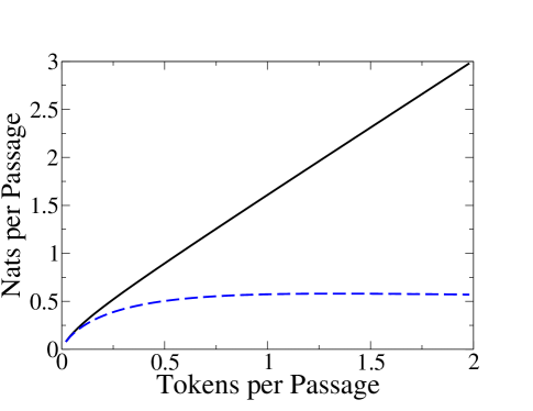
In FIGURE 4 we use Theorem 14 and Theorem 15 to plot lower and upper bounds for versus , a proxy for power budget, assuming some unit cost per token (). It is important to note that first-passage time variance (jitter) produces disordered tokens. That is, the mean first-passage time is only a measure of channel latency – the “propagation delay” so to speak – and does not itself impact token order uncertainty. However, for exponential first-passage the standard deviation also happens to be the first passage time . At small values of the bounds are tight. At larger the bounds diverge and the upper bound offers the tantalizing hint that timing channel capacity increases with increased token load (see also [8, 9]). Unfortunately, we have as yet been unable to find an empirical density which displays capacity growth similar to the upper bound and suspect that timing capacity flattens with increasing owing to a more rapidly increasing probability of token confusion at the output.
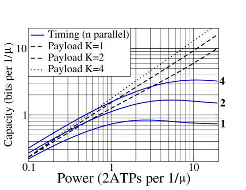
In FIGURE 5, we use Theorem 14 to plot lower bounds in bits per first-passage time, , as a function of power budget assuming DNA-based tokens. For token timing plus token payload signaling we show plots for DNA-residue tokens. For timing-only signaling we also include plots where different identifiable tokens (different molecule types or physically separate channels) are used (i.e., parallel timing channels as shown) for comparison with payload channels. We have assumed costs ATP. Furthermore, we assume since it seems likely that the absolute minimum energy for token release, , in a purely diffusive channel is probably comparable to the cost of creating (or breaking) the covalent bond used to append a nucleotide residue. If we assume ms, then the ordinate of FIGURE 5 is in kbit/s and the abscissa is in units of W. If , (as might be the case for smaller gaps in a nano-system) the ordinate is in and the abscissa is in units of W. These data rates are many many orders of magnitude larger than the fractional bit/second data rates previously reported for simple demonstrations of molecule communication [56], and the predicted power efficiencies are startling. Comparison of our results to [56] and others would be relatively straightforward if passage time jitter for the experimental setup were provided, although in [56] Avogradrian numbers of molecules were release with each alcohol “puff” so precise timing at the molecular level was not attempted.
Finally, it is worth noting that increasing the rate at which tokens with payload are launched will increase the bit rate but not increase the required energy per bit. Of particular note, at low power, timing-only signaling provides the best rates while at higher power, inscribed matter tokens may be preferred. However, if it is difficult to synthesize long strings (heavily information-laden tokens), even a single bit of information (two distinguishable species used in parallel) markedly increases capacity.
VI Discussion & Conclusion
We have provided a general and fundamental mathematical framework for molecular channels and derived some associated capacity bounds. We now discuss the results in the context of selected prior work and also touch upon ideas for further work suggested by the results. We separate these into two tranches:
-
•
Engineering Implications where we consider how molecular communication can be extended to other known communication scenarios as well where we might look for inspiration from biology that has had eons to evolve solutions.
-
•
Biological Implications where we consider how the results might impact/support known biology and suggest new avenues for investigation.
VI-A Engineering Implications
Capacity Bounds and Coding Methods: Our upper bound on capacity , the timing capacity for identical tokens, is tight for low token load but diverges for large . However, no empirical distributions with rates higher than the lower bound have yet been found. So, does the capacity of the timing-only channel truly flatten with increasing as in FIGURES 5 and 4, or is there a benefit to increasing the intensity of timing-token release as suggested in [8, 9]? In addition, since exponential first-passage is not the worse case corruption, what is the minmax capacity of the molecular timing channel? Likewise, how much better than exponential might be other first-passage densities imposed by various physical channels, and what are good codes for reliable transmission of information over molecular channels?
While we have focused on tokens in the form of linear symbolic strings, DNA and protein sequences in particular, what benefits might string tokens with a branched structure, exemplified by carbohydrates, confer for sequencing and/or payload? Should we vigorously pursue technology to produce large payload (many residue) tokens [57], or should a pool of smaller pre-fabricated payloads be used to deliver information? The bunching seen in FIGURE 5 for payload tokens with increasing may suggest the latter when rapid token construction is difficult. That is, the capacity per power output does not scale linearly in owing to the increased power required by adding more bases to tokens. This implies a tradeoff between timing-only and increasingly larger payloads – completely aside from the fact that payload size, shape and composition can have an effect on transport properties.
Precise Timing, Fuzzy Timing and Concentration: Of particular importance is establishing a careful quantitative relationship between our finest-grain timing model and other less temporally precise ones [37, 38, 1, 2, 3, 39, 4, 5, 6, 7, 40]. To begin, consider that our model seems to imply infinitely precise control over the release times and infinite precision measurement of the arrival times . However, release time and measurement time imprecision are both easily incorporated into the transit time vector . Thus, application of our model to the “fuzzier” release and detection times associated with practical/real systems is straightforward. Put another way, first passage time jitter already imposes limits on timing precision. Thus, so long as timing precision is significantly better than passage time jitter, the bounds presented here will be moderately tight. In addition, we are hopeful that the upper bound of Theorem Theorem 15 will be useful for evaluating molecular timing channel capacity for arbitrary first passage time distributions since it requires only knowledge of the timing channel capacity coupled to average properties of the corresponding input distribution.
Concentration is derived from considering temporal windows and counting the arrivals within them. Therefore, via the data processing theorem, our precise timing model must undergird all concentration-based methods which, even with perfect concentration detection, cannot possibly exceed the capacity of the finest grain timing model presented here. Of particular note for the asymptotic nature of our analysis here, an individual emission schedule for large is exactly a temporal emission concentration sequence as time resolution coarsens. That said, we have not as yet tried to show a graceful degradation toward coarse timing concentration from precise timing. Regardless, the results here provide crisp bounds on the capacities derived from concentration-based models.
As a specific example, there are channel models where information is carried by the number of molecules released and received (most recently, see [9, 58]). In this case, the capacity per channel use, , is upper bounded by since between and tokens can be released during a symbol interval of duration . Smaller increases the capacity in bits per second. Larger increases the capacity in bits per channel use.
If we assume a fixed signaling interval during which tokens are emitted, then we can also fix the average token rate as a proxy for power. Assuming a uniform distribution on the number of tokens sent we then have
| (77) |
since the average number of tokens released is .
Assuming exponential first passage, the probability that all tokens arrive by is minimized when all tokens are launched at . For exponential first passage and with arrival probability criterion as in section IV-A we have
| (78) |
which assures that even when tokens are emitted, they will all arrive before with probability .
However, equation (78) in combination with the power limit of equation (77) sets to
| (79) |
Then, since , after setting a successful channel use criterion of we have
| (80) |
which we rewrite as
| (81) |
with normalized power constraint
| (82) |
However, except for small , is not a reliable indicator of capacity since with increased , decreases but the probability of intersymbol interference (ISI) increases. Since calculating the capacity of this channel with ISI is difficult, we roughly approximate by normalizing by the expected number of intervals over which a given emission burst of tokens will span (thereby corrupting potentially them). Noting that is the probability that all tokens arrive before the end of the interval after emission we have
| (83) | |||||
and we obtain
| (84) | |||||
as an approximation to capacity for the number/concentration channel.
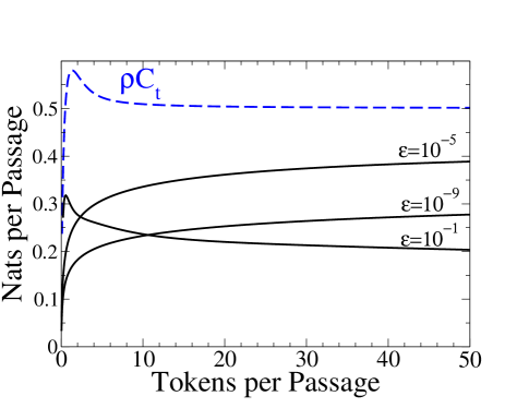
In FIGURE 6 we plot the upper bound of in equation (84) versus (i.e., parametrized in ) for a range of as compared to the timing channel lower bound in FIGURE 4. The timing channel capacity lower bound is always significantly greater than . Nonetheless, the coding simplicity of the number/concentration channel could make it an attractive option.
Identifiable Tokens Without Payload: In section IV-F we mentioned the possibility of uniquely identifying each of emitted tokens with a sequence number of length bits. We treat this scenario as distinct from ensemble timing channel coding which resolves residual orderering ambiguity (see section IV-F) because if the tokens are individually identifiable, the potential emission schedules are not constrained to ensemble timing channel coding. Thus, the identifiable tokens constitute parallel single-token timing channels, which for exponential first passage have aggregate capacity .
However, is limited by the power budget (in units of energy per passage, )
| (85) |
because each token requires bits of sequencing information energy. Following IV-A we have so the capacity in nats per passage time is
| (86) |
the last inequality owed to equation (85). However, in the limit of we have so we have
| (87) |
in units of nats per passage time (and assuming unit per-bit cost of the token identfier string). Thus, the identifiable token timing channel capacity exceeds the identical token timing channel lower bound with increasing power budget and scales linearly in power as does the timing channel upper bound (see FIGURE 4) – while still lying below it.
Token Corruption and Receptor Noise: Certain channel properties we have so far ignored must also be studied, such as the potential for lost or corrupted tokens and potential binding noise at receptor sites. However, as previously stated, token erasure (tokens which do not arrive) or payload token corruption (tokens which are altered in passage) or receptor noise (tokens bind stochastically to the receptor) can only decrease capacity (via the data processing theorem). Thus, the results here provide upper bounds. Nonetheless it is worth considering how the analytic machinery developed might be modified to take into account such impediments.
First, consider alteration of payload-carrying tokens en route. If the corruption is i.i.d. for each token, then the usual error correcting coding methods can be applied individually, or to the token ensemble. The resulting overall channel capacity will be degraded by the coding overhead necessary to preserve payload message integrity (including the sequencing headers).
Then consider token erasure where a token never arrives (and is assume to not arrive in a later signaling interval). Since each signaling interval uses tokens, we will know whether tokens get “lost” in transit and can arbitrarily assign a faux arrival time to such tokens. However, the problem this poses for our analysis is two-fold. First, tokens released later in the signaling interval are more likely to be lost which implies that the first passage density is not identical for each token. Second, the first passage density for each token would then contain a singularity equal to the probability of loss, violating one of our key assumptions and making hypersymmetric probability density folding arguments invalid. That said, an erasure channel approach where tokens were deleted randomly from the output could be pursued and owing to its i.i.d. nature (with respect to which tokens were erased) would likely provide a worst case scenario, since the information associated with erasures being more likely to be derived from a later release would be absent.
Finally, we have previously mentioned that a token may “arrive” multiple times owing to receptor binding kinetics. It was previously shown that given the first binding (first-passage) time the information content of subsequent bindings by the same token is nil [39]. In addition, as shown in section IV-A, information-theoretically patent channel use requires that tokens from a given emission interval be eventually cleared at the receiver. Otherwise, lingering tokens can interfere with subsequent emission intervals.
So, one could imagine that the rebinding process results in a characteristic finite-mean “burst” of arrivals associated with a given token which could perhaps be resolved into a single first-arrival time estimate – effectively adding more jitter to the first-passage time . If so, our model applies directly with appropriate modification. However, we have not attempted to analyze this scenario nor quantify the associated estimation noise. Thus, our results are most appropriately applied to systems where ligands bind tightly or where tokens are removed with high probability after first capture/detection. The addition of noisy ligand binding can only depress the capacity bounds presented here and we leave the question of exactly how much to future work.
Interference and Multiple Users: Multi-user communication in a molecular setting is a critical question, and a better understanding of the single-user channel will certainly help with multi-user studies where transmissions interfere. There is some work to inspire an information-theoretic edifice [59] similar to how the current work builds on [42], but the multi-user molecular signaling problem has not yet been rigorously considered. Of particular interest would be a version of MIMO since FIGURE 5 shows capacity benefits to parallel channels. One could imagine apposed arrays of emitters and receivers which could be engineered to collaborate to encode and decode information in a variety of ways, from parallel non-interfering channels to grossly interfering channels where joint/distributed coding might be employed. One could even imagine channels with chemically reactive species in which emitted tokens elicited spatially structured propagation of detectable reaction products [60, 61, 62].
Other Applications: It is interesting to note that although our work is couched in terms of molecular communication, the notion of token inscription applies to any system where discrete emissions experience random transport delay between sender and receiver. The most obvious example is the Internet where packets experience variable delay and may arrive out of order. Our results provide crisp bounds on the amount of sequencing overhead necessary for proper message reconstruction and even suggest that (at least for low payload packets traveling over independent routes) timing information could be an interesting adjunct to payload, depending upon the amount of timing jitter between the source and destination.
There is also the potential for cross pollination from biology to communication systems. As a simple example, there may be some selective benefit to hiding information from competitors. So, perhaps biological systems, where signaling chemicals are often detectable by other organisms, convey secrets over molecular communication channels in ways that can be mimicked in engineered systems. An obvious application, biosteganography [63], comes to mind in the context of tokens with payloads, although in such schemes timing plays no role as yet.
VI-B Biological Implications
Clearly, the natural world clearly offers a dizzying array of processes and phenomena through which the same and different tasks, communication or otherwise, might be accomplished (see, for example, [64, 65, 66, 67, 68, 69]). It is no wonder therefore that communication theorists have plied their trade heavily in this scientific domain (for a relatively recent review, see [70]). Identifying the underlying mechanisms (signaling modality, signaling agent, signal transport, and so on) as well as the molecules and structures implementing the mechanisms is no small undertaking. Consequently, experimental biologists use a combination of prior knowledge and what can only be called instinct to choose those systems on which to expend effort. Guidance may be sought from evolutionary developmental biology – a field that compares the developmental processes of different organisms to determine their ancestral relationship and to discover how developmental processes evolved. Insights may be gained by using statistical machine learning techniques to analyze heterogeneous data such as the biomedical literature and the output of so-called “omics” technologies – genomics (genes, regulatory, and non-coding sequences), transcriptomics (RNA and gene expression), proteomics (protein expression), metabolomics (metabolites and metabolic networks), pharmacogenomics (how genetics affects hosts’ responses to drugs), physiomics (physiological dynamics and functions of whole organisms), and so on.
Frequently, the application of communication theory to biology starts by selecting a candidate system whose components and operations have been already elucidated to varying degrees using methods in the experimental and/or computational biology toolbox [71, 72] and then applying communication and/or information theoretic methods [70, 73, 74, 75, 69, 76, 77, 78]. However, we believe that communication theory in general and information theory in particular are not mere system analysis tools for biology but new lenses on the natural world [79]. Here, we have sought to demonstrate the potential of communication theory as an organizing principle for biology. That is, given energy constraints and some general physics of a problem, an information-theoretic treatment can be used to provide outer bounds on information transfer in a mechanism-blind manner. Thus, rather than simply elucidating and quantifying known biology, communication theory can winnow the plethora of possibilities (or even suggest new ones) amenable to experimental and computational pursuit. Likewise, general application of communication-theoretic principles to biology affords a new set of application areas for communication theorists.
Examples of the implications of our main communication theoretic results are as follows:
-
•
We have derived a model and methodology for determining the amount of information a system using chemical signaling can convey under given power constraints. Do (or How do) biological systems achieve this extremely – even outrageously – low value?
-
•
Using tokens with large payloads can be very efficient. Is one example of this the transmission of hereditary material such as a genome over evolutionary time scales (periods spanning the history of groups and species)?
-
•
If it is difficult to synthesize long strings (information-laden tokens), even a single bit of information (two distinguishable species) increases capacity. Is the transmission of hormones, semiochemicals and other small molecules over developmental time scales (periods spanning the life of individuals) indicative of some efficiency tradeoff?
-
•
Although the production rate of tokens can be increased, the channel capacity might not increase if tokens are emitted at intervals smaller than the variability of arrival time. Does the material through which tokens travel hold the key to addressing this and the aforementioned questions and problems about engineered systems – particularly the issues of concentration versus timing, token corruption and interference and multiple users? In biological systems, discrete particles propagate through a cornucopia of substances en route from the source to the target: solids, liquids, gases or plasmas in the biosphere, lithosphere, atmosphere, hydrosphere, interstellar space or intergalactic space – for instance cytoplasm, nucleoplasm, mitochondrial matrix, extracellular matrix, extracellular polymeric substances, blood, lymph, phloem, xylem, bones, soil, rocks, air, water, steam, ice, and molecular clouds. Clearly, the “propagation delay” (jitter) experienced by a particular category and type of discrete particle is a function of the intrinsic physicochemical properties of the material. The standard deviation of arrival times will depend also on environmental factors such as temperature, pH, pressure and light.
Our results could guide studies aimed at answering three key questions biologists ask of a living organism: How does it work?, How is it built?, and How did it get that way? [80]. This is because our models of token timing, payload and timing+payload channels are inspired, at least in part, by fundamental “systems” problems about the dynamic and reciprocal relationship(s) between individuals in multicellular systems – whether microrganisms in communities or cells in metazoan tissues. Inscribed matter communication is a keystone of how individuals learn what to become or to be by a combination of internal and external cues and how, in turn, they teach others when to change or remain the same. Thus, the seemingly esoteric theoretical studies of channel capacities described here and discussed further in our companion paper might help pave the way to elucidating the origins (evolutionary developmental biology), generation (embryogenesis, and morphogenesis), maintenance (homeostasis, tolerance, and resilience), subversion (infectious and chronic diseases such as cancer and immune disorders), and decline (aging) of complex biological form and function [79].
A key virtue of the token timing model is its implicit acknowledgment of the importance of the “transmission medium” in the spatial gap between sender and receiver and through which tokens move. Consider molecular inscribed matter communication from the microscopic to the macroscopic levels: within and between cells in tissues and organisms in (agro)ecosystems. Since the presence of obstacles influences the mobility of discrete particles through a material, a crowded environment will increase the mean arrival time relative to unhindered diffusion but should have less of an impact on the mean emission time. Decades of laboratory in vitro studies have promulgated the view of the cellular interior as a place proteins, nucleic acids, carbohydrates, lipids and other molecules exist as highly purified entities that act in isolation, diffusing more or less freely until they find their cognate binding partner. In its natural milieu however, a molecule lives and operates in an extremely structured, complex and confining environment: one where it is surrounded by other molecules of the same or different chemical nature, the bystanders in the crowd having positive or negative effects on its mobility, biochemistry and cell biology [81, 82]. Widening the spatial and temporal horizon, semiochemicals diffusing through soil, water, and air mediate the complex ways crops, livestock, and microbes interact with one another.
Whether molecule release and capture occurs among organisms in the above- and below-ground environments or between cells in the tissue microenvironment, the basic physics is similar. For this reason we feel that our fundamental treatment of inscribed matter communication presented here could help guide biological understanding and experimentation.
Acknowledgments
Profound thanks are owed to A. Eckford, N. Farsad, S. Verdú and V. Poor for useful discussions and guidance. We are also extremely grateful to the editorial staff and the raft of especially careful and helpful anonymous reviewers. This work was supported in part by NSF Grant CDI-0835592.
References
- [1] A. Einolghozati, M. Sardari, A. Beirami, and F. Fekri. Capacity of Discrete Molecular Diffusion Channels. In IEEE International Symposium on Information Theory (ISIT) 2011, pages 603–607, July 2011.
- [2] Josep Miquel Jornet Ian F. Akyildiz and Massimiliano Pierobon. Nanonetworks: A New Frontier in Communications. Communications of the ACM, 54(11):84–89, 2011.
- [3] M. Pierobon and I. Akyildiz. Capacity of a diffusion-based molecular communication system with channel memory and molecular noise. IEEE Transactions on Information Theory, 59(2):942–954, 2013.
- [4] T. Nakano, A. W. Eckford, and T. Haraguchi. Molecular Communication. Cambridge University Press, 2013.
- [5] A. Einolghozati, M. Sardari, and F. Fekri. Relaying in diffusion-based molecular communication. In IEEE International Symposium on Information Theory 2013, pages 2959–2963, 2013.
- [6] A. Einolghozati, M. Sardari, and F. Fekri. Design and analysis of wireless communication systems using diffusion-based molecular communication among bacteria. IEEE Transactions on Wireless Communications, 12(12):6096–6105, 2013.
- [7] A. Einolghozati, M. Sardari, and F. Fekri. Decode and forward relaying in diffusion-based molecular communication between two populations of biological agents. In Information Conference on Communications, 2014 IEEE ICC, pages 3975–3980, 2014.
- [8] N. Farsad, Y. Murin, A. W. Eckford, and A. Goldsmith. On the Capacity of Diffusion-Based Molecular Timing Channels. In IEEE International Symposium on Information Theory 2016, pages 1023–1027, July 2016.
- [9] N. Farsad, Y. Murin, A. W. Eckford, and A. Goldsmith. Capacity Limits of Diffusion-Based Molecular Timing Channels. IEEE Transactions on Information Theory, 2016. in preparation for submission.
- [10] T.M. Cover and J.A. Thomas. Elements of Information Theory. Wiley-Interscience, 1991.
- [11] N. Michelusi and U. Mitra. Capacity of electron-based communication over bacterial cables: the full-CSI case. IEEE Transactions on Molecular, Biological and Multi-Scale Communications, 1(1):62–75, 2015.
- [12] C. Morris and D. Sands. From grains to rain: the link between landscape, airborne microorganisms and climate processes, 2012. http://bioice.wordpress.com/.
- [13] J.M. Houtkooper. Glaciopanspermia: Seeding the terrestrial planets with life? Planetary and Space Science, 59:1107–1111, 2011.
- [14] M. Küppers, L. O’Rourke, D. Bockelée-Morvan, V. Zakharov, S. Lee, P. von Allmen, B. Carry, D. Teyssier, A. Marston, T. Müller, J. Crovisier, M.A. Barucci, and R. Moreno. Localized sources of water vapour on the dwarf planet (1) Ceres. Nature, 505:525–527, 2014.
- [15] A. S. Tannenbaum. Computer Networks. Prentice Hall, 2002.
- [16] J. Gray, W. Chong, Barclay T, A. Szalay, and J. vandenBerg. TeraScale SneakerNet: Using Inexpensive Disks for Backup, Archiving, and Data Exchange. Technical Report MSR-TR-2002-54, Microsoft Research, May 2002. (http://research.microsoft.com/research/pubs).
- [17] S.J. Devitt, A.D. Greentree, A.M. Stephens, and R. Van Meter. High-speed quantum networking by ship. arXiv:1410.3224 [quant-ph], 2014.
- [18] R. H. Frenkiel and T. Imielinski. Infostations: The joy of ‘many-time, many-where’ communications. WINLAB-TR 119, WINLAB, Rutgers University, April 1996.
- [19] R. Song, C. Rose, Y-L Tsai, and I.S. Mian. Wireless Signaling with Identical Quanta. In IEEE WCNC, Paris, April 2012.
- [20] D. J. Goodman, J. Borras, N. B. Mandayam, and R. D. Yates. INFOSTATIONS : A New System Model for Data and Messaging Services . In Proceedings of IEEE VTC’97, volume 2, pages 969–973, May 1997. Phoenix, AZ.
- [21] J. Irvine, D. Pesh, D. Robertson, and D. Girma. Efficient UMTS Data Service Provision using Infostations. In Proceedings of the IEEE Vehicular Technology Conference, volume 3, pages 2119–2123, 1998.
- [22] D. J. Goodman, J. Borras, N. B. Mandayam, and R. D. Yates. Infostations: A New System Model for Data and Messaging Services. In Proceedings of the IEEE Vehicular Technology Conference, volume 2, pages 969–973, 1997.
- [23] J. Irvine and D. Pesh. Potential of DECT Terminal Technology for Providing Low-cost Wireless Internet Access through Infostations. In IEE Colloquium on UMTS Terminal and Software Radio, pages 12/1–6, 1999.
- [24] R. H. Frenkiel, B. R. Badrinath, J. Borras, and R. Yates. The Infostations Challenge: Balancing Cost and Ubiquity in Delivering Wireless Data. IEEE Personal Communications, 7(2):66–71, April 2000.
- [25] A. L. Iacono and C. Rose. Bounds on File Delivery Delay in an Infostations System. In Proceedings of the IEEE Vehicular Technology Conference, 2000.
- [26] A. Iacono and C. Rose. Infostations: New Perspectives On Wireless Data Networks. In Next Generation Wireless Networks. Kluwer Academic, May 2000. Editor: S. Tekinay.
- [27] A.L. Iacono. File Delivery Delay in and Infostations System. PhD thesis, Rutgers, The State University of New Jersey, New Brunswick, New Jersey, June 2000.
- [28] A. Iacono and C. Rose. Bounds on file delivery delay in an infostations system. In IEEE Vehicular Technology Conference, pages 6.11–3, May 2000. Tokyo.
- [29] A. Iacono and C. Rose. MINE MINE MINE: Information Theory, Infostation Networks and Resource Sharing. In WCNC 2000, September 2000. Chicago, IL.
- [30] F. Atay and C. Rose. Exploiting Mobility in Multi-hop Infostation Networks to Decrease Transmit Power. In IEEE WCNC’04, Atlanta, GA, March 2004.
- [31] F. Atay and C. Rose. Threshold Based Policies in Infostations Networks. In CISS’04, Princeton, NJ, March 2004.
- [32] C. Rose and G. Wright. Will ET Write or Radiate: inscribed mass vs. electromagnetic channels. In Asilomar, October 2004. Pacific Grove, CA.
- [33] C. Rose. Write or Radiate? In IEEE Vehicular Technology Conference, October 2003. Orlando.
- [34] C. Rose and G. Wright. Inscribed Matter As An Energy-Efficient Means Of Communication With An Extraterrestrial Civilization. Nature, 431:47–49, 2004.
- [35] S. Goforth. NSF Discoveries: Getting a Message Across the Universe: Would E.T. Send a Letter? . http://www.nsf.gov/discoveries/disc_summ.jsp?cntn_id=106711&org=CCF.
- [36] IEEE. IEEE Transactions on Molecular Biological and Multi-Scale Communications. Editors: U. Mitra and A. Eckford.
- [37] B. L. Bassler. How bacteria talk to each other: regulation of gene expression by quorum sensing. Curr Opin Microbiol, 2(6):582–587, Dec 1999.
- [38] B.L. Bassler. Small talk: cell-to-cell communication in bacteria. Cell, 109(4):421–424, May 2002.
- [39] A.W. Eckford. Nanoscale communication with Brownian motion. In CISS’07, pages 160–165, 2007. Baltimore.
- [40] It’s the Alcohol Talking. The Economist, March 2014. Technology Quarterly: monitor.
- [41] C. Rose and I.S. Mian. A Fundamental Framework for Molecular Communication Channels: timing & payload. In IEEE International Conference on Communications, pages 1043–1048, June 2015. London.
- [42] V. Anantharam and S. Verdu. Bits Through Queues. IEEE Transactions on Information Theory, 42(1):4–18, January 1996.
- [43] R. Sundaresan and S. Verdú. Robust Decoding for Timing Channels. IEEE Transactions on Information Theory, 46(2), 2000.
- [44] R. Sundaresan and S. Verdú. Capacity of Queues Via Point-Process Channels. IEEE Transactions on Information Theory, 52(6), 2006.
- [45] C. Rose, R. Song, and I.S. Mian. Timing Channels with Multiple Identical Quanta. IEEE Transactions on Information Theory, 2013. (in preparation, available: http://arxiv.org/abs/1208.1070).
- [46] C. Rose and I.S. Mian. Signaling with identical tokens: Lower bounds with energy constraints. In IEEE International Symposium on Information Theory (ISIT’13), pages 1839–1843, July 2013.
- [47] C. Rose and I.S. Mian. Signaling with identical tokens: Upper bounds with energy constraints. In IEEE International Symposium on Information Theory (ISIT’14), pages 1817–1821, June 2014.
- [48] C. Rose and I.S. Mian. Inscribed Matter Communication: Part II. IEEE Transactions Molecular, Biological and Multiscale Communication, 2016. (revised, Nov. 21) ArXiv: http://arxiv.org/abs/1606.05036.
- [49] Y-L Tsai, C. Rose, R. Song, and I.S. Mian. An Additive Exponential Noise Channel with a Transmission Deadline. In IEEE International Symposium on Information Theory (ISIT’11), pages 598–602, July 2011.
- [50] A. Papoulis. Probability, Random Variables, and Stochastic Processes. McGraw-Hill, New York, third edition, 1991.
- [51] F.B. Hildebrand. Advanced Calculus for Applications. Prentice Hall, Englewood Cliffs, NJ, 1976.
- [52] F.P. Brooks Jr. Three great challenges for half-century-old computer science. J. ACM, 50:25–26, 2003.
- [53] R.G. Gallager. Information Theory and Reliable Communication. Wiley, 1968.
- [54] D.L. Nelson and M.M. Cox. Lehninger Principles of Biochemistry. Freeman, 2005. 4th Ed.
- [55] T. Tugcu M.S. Kurana, H.B. Yilmaz and B. Ozerman. Energy model for communication via diffusion in nanonetworks. Nano Communication Networks, 1:86–95, 2010.
- [56] C. Lee, B. Koo, N-R Kim, G. Yilmaz, N. Farsad, A. Eckford, and C-B Chae. Molecular MIMO Communication Link. March 2015. arXiv:1504.04921v2 [cs.ET].
- [57] G.S. Sandhu G.M. Church V. Zhirnov, R.M. Zadegan and W.L. Hughes. Nucleic Acid Memory. Nature Materials, 15:366–370, April 2016.
- [58] A. Eckford C. B. Chae N. Farsad, H. B. Yilmaz and W. Guo. A Comprehensive Survey Of Recent Advancements In Molecular Communication. IEEE Communications Surveys Tutorials, 18(3):1887–1919. 3rd Quarter, 2016.
- [59] G. C. Ferrante, T. Q. S. Quek, and M. Z. Win. An achievable rate region for superposed timing channels. In 2016 IEEE International Symposium on Information Theory (ISIT), pages 365–369, July 2016.
- [60] Kapral, R. and Showalter, K. Chemical Waves and Patterns. Springer, 1995.
- [61] B.H. Gilding and R. Kersner. Travelling Waves in Nonlinear Diffusion Convection Reaction. Birkhauser, 2004.
- [62] P.C Fife. Mathematical Aspects of Reacting and Diffusing Systems. Springer, 1979.
- [63] T.D.P. Brunet. Aims and methods of biosteganography. J. Biotechnology, 226(20):56–64, May 2016.
- [64] C. de Joussineau, J. Soule, M. Martin, C Anguille, P. Montcourrier, and D. Alexandre. Delta-Promoted Filopodia Mediate Long-Range Lateral Inhibition in Drosophila. Nature, 426:555–559, December 4 2003.
- [65] Y.A. Gorby, S. Yanina, JS.. McLean, K.M. Rosso, D. Moyles, A. Dohnalkova, T.J. Beveridge, I.S. Chang, B.H. Kim, K.S. Kim, D.E. Culley, S.B. Reed, M.F. Romine, D.A. Saffarini, E.A. Hill, L. Shi, D.A. Elias, D.W. Kennedy, G. Pinchuk, K. Watanabe, S. Ishii, B. Logan, K.H. Nealson, and J.K. Fredrickson. Electrically conductive bacterial nanowires produced by Shewanella oneidensis strain MR-1 and other microorganisms. Proc Natl Acad Sci U.S.A., 103:11358–11363, 2006.
- [66] S. Gurke, J.F.V. Barroso, and H.-H. Gerdes. The art of cellular communication: tunneling nanotubes bridge the divide. Histochem Cell Biol, 129:539–550, 2008.
- [67] X. Wang, M.L. Veruki, N.V. Bukoreshtliev, E. Hartveit, and H.-H. Gerdes. Animal cells connected by nanotubes can be electrically coupled through interposed gap-junction channels. Proc Natl Acad Sci USA, 107:17194–17199, 2010.
- [68] H.C. Berg and E.W. Purcell. Physics of Chemoreception. Biophysical Journal, 20:193–219, 1977.
- [69] P. Mehta, S. Goyal, T. Long, B.L. Bassler, and N.S. Wingreen. Information processing and signal integration in bacterial quorum sensing. Mol Syst Biol, 5:325, 2009.
- [70] O. Milenkovic, G. Alterovitz, G. Battail, T. P. Coleman, J. Hagenauer, S. P. Meyn, N. Price, M. F. Ramoni, I. Shmulevich, and W. Szpankowski. Introduction to the special issue on information theory in molecular biology and neuroscience. Trans. Information Theory, 56(2):649–652, 2010.
- [71] A.L. Hodgkin and A.F. Huxley. A quantitative description of membrane current and its application to conduction and excitation in nerve. J. Physiol., 117(4):500–544, 1952.
- [72] T. Long, K.C. Tu, Y. Wang, P. Mehta, N.P. Ong, B.L. Bassler, and N.S. Wingreen. Quantifying the integration of quorum-sensing signals with single-cell resolution. PLoS Biol, 24:e68, 2009.
- [73] E. Wajnryb J.M. Amigo, J. Szczepanski and M.V. Sanchez-Vives. Estimating the entropy rate of spike trains via lempel-ziv complexity. Neural Computation, 16:717–736, 2004.
- [74] D.H. Johnson. Information Theory and Neural Information Processing. Trans. Information Theory, 56(2):653–666, Feb 2010.
- [75] R. Barbieri, L.M. Frank, D.P. Nguyen, M.C. Quirk, V., M.A. Wilson, and E.N. Brown. Dynamic analyses of information encoding in neural ensembles. Neural Computation, 16:277–307, 2004.
- [76] Z. Mousavian, J. Díaz, and A. Masoudi-Nejad. Information theory in systems biology. Part II: protein-protein interaction and signaling networks. Semin Cell Dev Biol, 51:14–23, 2016.
- [77] Masoudi-Nejad A. Mousavian Z, Kavousi K. Information theory in systems biology. Part I: Gene regulatory and metabolic networks. Semin Cell Dev Biol, 51:3–13, 2016.
- [78] S. Uda and S. Kuroda. Analysis of cellular signal transduction from an information theoretic approach. Semin Cell Dev Biol, 51:24–31, 2016.
- [79] I.S. Mian and C. Rose. Communication theory and multicellular biology. Integrative Biology, 3(4):350–367, April 2011.
- [80] S. Brenner. Turing centenary: Life’s code script. Nature, 482:461, 2012.
- [81] S. Mittal, R.K. Chowhan, and L.R. Singh. Macromolecular crowding: Macromolecules friend or foe. Biochim Biophys Acta, 1850:1822–1831, 2015.
- [82] I.M. Kuznetsova, B.Y. Zaslavsky, L. Breydo, K.K. Turoverov, and V.N. Uversky. Beyond the excluded volume effects: mechanistic complexity of the crowded milieu. Molecules, 20:1377–1409, 2015.