Inversion Copulas from Nonlinear State Space Models with Application to Inflation Forecasting

$\mbox{}^{\star}$ Corresponding author: Assistant Professor Ole Maneesoonthorn, Melbourne Business School, 200 Leicester Street, Carlton, VIC, 3053, Australia. Email: O.Maneesoonthorn@mbs.edu.

Inversion Copulas from Nonlinear State Space Models with Application to Inflation Forecasting
Abstract

We propose to construct copulas from the inversion of nonlinear state space models. These allow for new time series models that have the same serial dependence structure of a state space model, but with an arbitrary marginal distribution, and flexible density forecasts. We examine the time series properties of the copulas, outline serial dependence measures, and estimate the models using likelihood-based methods. Copulas constructed from three example state space models are considered: a stochastic volatility model with an unobserved component, a Markov switching autoregression, and a Gaussian linear unobserved component model. We show that all three inversion copulas with flexible margins improve the fit and density forecasts of quarterly U.S. broad inflation and electricity inflation.

Keywords: Copulas; Nonlinear Time Series; Bayesian Methods; Nonlinear Serial Dependence; Density Forecasts; Inflation Forecasting.

1 Introduction

Parametric copulas constructed through the inversion of a latent multivariate distribution (Nelsen 2006, sec. 3.1) are popular for the analysis of high-dimensional dependence. For example, Gaussian (Song 2000), t (Embrechts, McNeil & Straumann 2001) and skew t (Demarta & McNeil 2005; Smith, Gan & Kohn 2012) distributions have all been used to form such ‘inversion copulas’. More recently, Oh & Patton (2015) suggest employing distributions formed through marginalization over a small number of latent factors. However, the copulas constructed from these distributions cannot capture accurately the serial dependence exhibited by many time series. As an alternative, we instead propose a broad new class of inversion copulas formed by inverting parametric nonlinear state space models. Even though the dimension of such a copula is high, it is parsimonious because its parameters are those of the underlying latent state space model. The copula also has the same serial dependence structure as the state space model. But when such copulas are combined with an arbitrary marginal distribution for the data, they allow for the construction of new time series models. These models allow for substantially more flexible density forecasts than the underlying state space models themselves, because the latter typically have rigid margins that are often inconsistent with that observed empirically.

When the latent state space model is non-stationary, the resulting copula model for the data is also, but with time invariant univariate margins. Alternatively, when the state space model is stationary, so is the resulting copula model, and we focus on this case here. When the state space model is Gaussian and linear, the resulting inversion copula is a Gaussian copula (Song 2000) with a closed form likelihood. However, in general, the likelihood function of a nonlinear state space model cannot be expressed in closed form. Similarly, neither can the density of the corresponding inversion copula. Nevertheless, we show how existing techniques for computing the likelihood of such state space models can also be used to compute the copula densities. We also provide an efficient spline approximation method for computing the marginal density and quantile function of the state space model. These are the most computationally demanding aspects of evaluating the copula density for time series data. We outline in detail how Bayesian techniques can be used to compute posterior estimates of the copula model parameters. A Markov chain Monte Carlo (MCMC) sampler is used, where the existing methods for efficiently sampling the states of a state space model can be employed directly. We also study the time series properties of the copula models, show how to compute measures of serial dependence, as well as construct density forecasts. We show that the density forecasts from the copula model better reflect the nature of the empirical data distribution than the state space model counterpart in real world applications.

Copula models are used extensively to model cross-sectional dependence, including between multiple time series; see Patton (2012) for a review. However, their use to capture serial dependence is much more limited. Joe (1997, pp.243-280), Lambert & Vandenhende (2002), Frees & Wang (2006), Beare (2010), Smith, Min, Almeida & Czado (2010) and Loaiza-Maya, Smith & Maneesoonthorn (2017) use Archimedean, elliptical or decomposable vine copulas to capture serial dependence in univariate time series. While the likelihood is available in closed form for these copulas, they cannot capture as wide a range of serial dependence structures as the inversion copulas proposed here can. Moreover, the proposed inversion copulas are simple to specify, often more parsimonious, and can be easier to estimate than the copulas used previously.

Recently, copulas with time-varying parameters have proven popular for the analysis of multivariate time series data; for example, see Almeida & Czado (2012), Hafner & Manner (2012), De Lira Salvatierra & Patton (2015) and Creal & Tsay (2015). However, these authors use copulas to account for the (conditional) cross-sectional dependence as in Patton (2006). This is completely different to our objective of constructing a $T$-dimensional copula for serial dependence. Semi- and nonparametric copula functions (Kauermann, Schellhase & Ruppert 2013) can also be used to model serial dependence. However, such an approach is better suited to longitudinal data, where there are repeated observations of the time series.

To highlight the broad range of new copulas that can be formed using our approach, we consider three in detail. They are formed by inversion of three stationary latent state space models that are popular in forecasting macroeconomic time series. The first is a stochastic volatility model with an unobserved first order autoregressive mean component. The second is a Markov switching first order autoregression. The third is a Gaussian unobserved component model, where the unobserved component follows a $p$th order autoregression. When forming an inversion copula, all characteristics (including moments) of the marginal distribution of the state space model are lost, leaving the parameters potentially unidentified. For each of the three inversion copulas we study in detail, we solve this problem by imposing constraints on the parameter space. We show how to implement the MCMC sampling scheme, where the states are generated using existing methods, and the parameters are drawn efficiently from constrained distributions. In an empirical setting, we also show how to estimate the copula parameters using maximum likelihood.

To show that that using an inversion copula with a flexible margin can substantially improve forecast density accuracy, compared to employing the state space model directly, we use it to model and forecast quarterly U.S. broad inflation and U.S. electricity inflation. This is a long-standing problem on which there is a large literature (Faust & Wright 2013). A wide range of univariate time series models have been used previously, including the three state space models examined here. However, all three have marginal distributions that are inconsistent with that observed empirically for inflation, which exhibits strong positive skew and heavy tails. Moreover, the predictive distributions from the state space models are either exactly or approximately symmetric– a feature that places excessively high probability on severe deflation. In comparison, the inversion copula models can employ the same serial dependence structure as the latent state space models, but also incorporate much more accurate asymmetric marginal distributions. We show that this not only improves the fit of the time series models, but that it increases the accuracy of the one-quarter-ahead density forecasts significantly.

The rest of the paper is organized as follows. In Section 2 we first define a time series copula model, and then outline the construction of an inversion copula from a nonlinear state space model. The special case of a Gaussian linear state space model is considered separately. We then discuss estimation, time series properties, measures of serial dependence and prediction. In Section 3 we discuss the three inversion copulas that we examine in detail, while in Section 4 we present the analyses of the U.S. broad inflation and U.S. electricity inflation; Section 5 concludes. In a supplementary appendix, we provide a simulation study that verifies the proposed methodology in a controlled setting (Section A), as well as supplementary figures for the U.S. electricity inflation application (Section B).

2 Time Series Copula Models

Consider a discrete-time stochastic process $\{Y_{t}\}_{t=1}^{T}$, with a time series of observed values $\bm{y}=(y_{1},\ldots,y_{T})$. Then a copula model decomposes its joint distribution function as

$$F_{Y}(\bm{y})=C(\bm{u})\,.$$ (2.1)

Here, $\bm{u}=(u_{1},\ldots,u_{T})$, $u_{t}=G(y_{t})$, and $G$ is the marginal distribution function of $Y_{t}$, which we assume to be time invariant. The function $C$ is a $T$-dimensional copula function (Nelsen 2006, p.45), which captures all serial dependence in the data. All marginal features of the data are captured by $G$, which can be modeled separately, and either parametrically or non-parametrically. While Equation (2.1) applies equally to both continuous and discrete-valued time series data, we focus here on the former, where the density

$$f_{Y}(\bm{y})=\frac{d}{d\bm{y}}F_{Y}(\bm{y})=c(\bm{u})\prod_{t=1}^{T}g(y_{t})\,.$$ (2.2)

Here, $g(y)=\frac{d}{dy}G(y)$ is the marginal density of each observation, and $c(\bm{u})=\frac{d}{d\bm{u}}C(\bm{u})$ is widely called the ‘copula density’.

We refer to Equations (2.1) and (2.2) as a ‘time series copula model’. The main challenge in constructing such a model is the selection of an appropriate copula function $C$. It has to be both of high dimension, and also account accurately for the potentially complex serial dependence structure in $\{Y_{t}\}_{t=1}^{T}$.

2.1 State Space Inversion Copula

A popular way to construct a high-dimensional copula $C$ is by transformation from a latent continuous-valued stochastic process $\{Z_{t}\}_{t=1}^{T}$, with joint distribution function $F_{Z}$. Let $F_{Z_{t}}$ be the marginal distribution function of $Z_{t}$. Then, by setting $U_{t}=F_{Z_{t}}(Z_{t})$, the $T$ observations of the stochastic process $\{U_{t}\}_{t=1}^{T}$ have distribution function

$$C(\bm{u})=F_{Z}(F_{Z_{1}}^{-1}(u_{1}),\ldots,F_{Z_{T}}^{-1}(u_{T}))\,,$$

and density function

$$c(\bm{u})=\frac{f_{Z}(\bm{z})}{\prod_{t=1}^{T}f_{Z_{t}}(z_{t})}\,,$$ (2.3)

where $z_{t}=F_{Z_{t}}^{-1}(u_{t})$, $\bm{z}=(z_{1},\ldots,z_{T})$, $f_{Z}(\bm{z})=\frac{d}{d\bm{z}}F_{Z}(\bm{z})$, and $f_{Z_{t}}(z_{t})=\frac{d}{dz_{t}}F_{Z_{t}}(z_{t})$. The transformation ensures that each $U_{t}$ is marginally uniformly distributed on $[0,1]$, so that $C$ meets the conditions of a copula function (Nelsen 2006, p.45).

This approach to copula construction is called inversion by Nelsen (2006, sec. 3.1), and we label such a copula an ‘inversion copula’. Table 1 depicts the transformations between $Y_{t}$, $U_{t}$ and $Z_{t}$, along with their distribution functions and domains. Previous choices for $F_{Z}$ include elliptical (especially the Gaussian and t), skew t distributions and latent factor models (Oh & Patton 2015). The dependence properties of the resulting inversion copulas are inherited from those of $F_{Z}$, although all location, scale and other marginal properties of $F_{Z_{t}}$ are lost in the transformation. In this paper we propose to construct an inversion copula from a latent nonlinear state space model for $\{Z_{t}\}_{t=1}^{T}$. In doing so, we aim to construct new high-dimensional copulas that inherit the rich range of serial dependence structures that state space models allow.

The nonlinear state space model we consider is generically given by

$$Z_{t}|\bm{X}_{t}=\bm{x}_{t} \sim H_{t}(z_{t}|\bm{x}_{t};\bm{\psi})$$ (2.4)

$$\bm{X}_{t}|\bm{X}_{t-1}=\bm{x}_{t-1} \sim K_{t}(\bm{x}_{t}|\bm{x}_{t-1};\bm{\psi}).$$ (2.5)

Here, $H_{t}$ is the distribution function of $Z_{t}$, conditional on a $r$-dimensional state vector $\bm{X}_{t}$. The states follow a Markov process, with conditional distribution function $K_{t}$. Parametric distributions are almost always adopted for $H_{t}$ and $K_{t}$, and we do so here with parameters we denote collectively as $\bm{\psi}$. In the time series literature Equations (2.4) and (2.5) are called the measurement and transition distributions, although in the copula context $Z_{t}$ is not directly observed, but is also latent. Note that even though the state vector $\bm{X}_{t}$ has Markov order one, $Z_{t}$ is Markov with an arbitrary order; see Durbin & Koopman (2012) for properties of this model.

A key requirement in evaluating the inversion copula density at Equation (2.3) is computing the marginal distribution and density functions of $Z_{t}$. These are given by

$$F_{Z_{t}}(z_{t}|\bm{\psi}) = \int H_{t}(z_{t}|\bm{x}_{t};\bm{\psi})f(\bm{x}_{t}|\bm{\psi})\mbox{d}\bm{x}_{t}$$

$$f_{Z_{t}}(z_{t}|\bm{\psi}) = \int h_{t}(z_{t}|\bm{x}_{t};\bm{\psi})f(\bm{x}_{t}|\bm{\psi})\mbox{d}\bm{x}_{t}\,,$$ (2.6)

where the dependence on $\bm{\psi}$ is denoted explicitly here. The density $h_{t}(z_{t}|\bm{x}_{t};\bm{\psi})=\frac{d}{dz_{t}}H_{t}(z_{t}|\bm{x}_{t};\bm{\psi})$, and $f(\bm{x}_{t}|\bm{\psi})$ is the marginal density of the state variable $\bm{X}_{t}$ which can be derived analytically from the transition distribution for most state space models used in practice. Evaluation of the integrals in Equation (2.6) is typically straightforward either analytically or numerically, as we show later for three different state space models. Note that $z_{t}$ is a function of $\bm{\psi}$ through the quantile function $z_{t}=F^{-1}_{Z_{t}}(u_{t}|\bm{\psi})$, as we discuss later.

A more challenging problem is the evaluation of the numerator in Equation (2.3). To compute this, the state vector $\bm{x}=(\bm{x}_{1},\ldots,\bm{x}_{T})$ needs to be integrated out, with

$$f_{Z}(\bm{z}|\bm{\psi}) = \int f(\bm{z}|\bm{x},\bm{\psi})f(\bm{x}|\bm{\psi})\mbox{d}\bm{x}$$

$$= \int\prod_{t=1}^{T}h_{t}(z_{t}|\bm{x}_{t};\bm{\psi})\prod_{t=2}^{T}k_{t}(\bm{x}_{t}|\bm{x}_{t-1};\bm{\psi})f(\bm{x}_{1};\bm{\psi})\mbox{d}\bm{x}\,,$$

where $k_{t}(\bm{x}_{t}|\bm{x}_{t-1};\bm{\psi})=\frac{d}{d\bm{x}_{t}}K_{t}(\bm{x}_{t}|\bm{x}_{t-1};\bm{\psi})$. There are many methods suggested for evaluating this high-dimensional integral; for example, see Shephard & Pitt (1997), Stroud, Müller & Polson (2003), Godsill, Doucet & West (2004), Jungbacker & Koopman (2007), Richard & Zhang (2007), Scharth & Kohn (2016) and references therein. In this paper we show how popular Markov chain Monte Carlo (MCMC) methods for solving this problem can also be used to estimate the inversion copula.

Because all features of the marginal distribution of $Z_{t}$— including the marginal moments— are lost when forming the copula, parameters in a state space model that uniquely affect these are unidentified and can be excluded from $\bm{\psi}$. Moreover, where possible we also impose constraints on the parameters so that $F_{Z_{t}}$ has zero mean and unit variance. While this has no effect on the copula function $C$, it aids identification of the parameters in the likelihood.

2.2 Gaussian Linear State Space Inversion Copula

The stationary Gaussian linear state space model encompasses many popular time series models; see Ljung (1999, Sec. 4.3) and Durbin & Koopman (2012, Part 1) for overviews. In this special case, we show here that the inversion copula is the popular Gaussian copula. This state space model is given by

$$Z_{t}|\bm{X}_{t}=\bm{x}_{t} \sim N(\bm{b}\bm{x}_{t}^{\prime},\sigma^{2})$$

$$\bm{X}_{t}|\bm{X}_{t-1}=\bm{x}_{t-1} \sim N(\bm{x}_{t-1}R^{\prime},FQF^{\prime}),$$ (2.7)

where $\bm{X}_{t}$ is a $(1\times r)$ state vector, $\bm{b}$ is a $(1\times r)$ vector, $\sigma^{2}$ is the disturbance variance, $R$ is a $(r\times r)$ matrix of autoregressive coefficients, with absolute values of all eigenvalues less than one. The matrices $F$ and $Q$ are of sizes $(r\times q)$ and $(q\times q)$, respectively, where $q$ represents the dimension of random components driving the $r$-dimensional state. The copula parameters are $\bm{\psi}\subseteq\{\bm{b},R,F,Q,\sigma^{2}\}$, depending on the specific state space model adopted.

To identify the parameters in the likelihood, they are constrained so that $E(Z_{t})=0$ and $\mbox{Var}(Z_{t})=1$. For the latter, if $\mbox{Var}(\bm{X}_{t})=\Sigma_{X}$, then $\mbox{Var}(Z_{t})=\bm{b}\Sigma_{X}\bm{b}^{\prime}+\sigma^{2}$, where $\mbox{vec}(\Sigma_{X})=(I_{r^{2}}-R\otimes R)^{-1}\mbox{vec}(FQF^{\prime})$. This results in the equality constraint $\sigma^{2}=1-\bm{b}\Sigma_{X}\bm{b}^{\prime}$, along with nonlinear inequality constraints on the other elements of $\bm{\psi}$; something we illustrate further for a specific Gaussian state space model in Section 3.3.

With these constraints, the margins of $Z_{t}$ are standard normal. This greatly simplifies evaluation and estimation of the copula compared to the general case, where $f_{Z_{t}}$ and $F_{Z_{t}}$ in Equation (2.6) depend on $\bm{\psi}$ and need to be recomputed whenever $\bm{\psi}$ changes. Moreover, $(Z_{1},\ldots,Z_{T})\sim N(\bm{0},\Omega_{\psi})$, with

$$\Omega_{\psi}=\begin{bmatrix}1&a_{1}&\dots&a_{T-1}\\ a_{1}&1&\dots&a_{T-2}\\ \vdots&\vdots&\ddots&\vdots\\ a_{T-1}&a_{T-2}&\dots&1\end{bmatrix},$$

where $a_{l}=\bm{b}\Gamma(l)\bm{b}^{\prime}$, and $\Gamma(l)=\mbox{Cov}(\bm{X}_{t},\bm{X}_{t-l})$ denotes the $l^{\mbox{\scriptsize th}}$ autocovariance matrix of the state vectors, which can be computed using the multivariate Yule-Walker equations (Lutkepohl 2006, pp.26–30).

Because this is a Gaussian copula, its density is known explicitly (Song 2000) as

$$c_{Ga}(\bm{u};\bm{\psi})=|\Omega_{\psi}|^{-1/2}\exp\left(-\frac{1}{2}\bm{z}(\Omega_{\psi}^{-1}-I)\bm{z}^{\prime}\right)\,.$$

The copula parameters $\bm{\psi}$ can therefore be estimated using the full likelihood in Equation (2.2). However, $\Omega_{\psi}^{-1}$ is usually computationally demanding to evaluate, so that $c_{Ga}(\bm{u};\bm{\psi})$ is also. Therefore, we instead employ Bayesian methods where the latent states are generated explicitly as part of a MCMC scheme, as we now discuss. This can be just as fast and efficient for the inversion copula, as it is for the underlying linear Gaussian state space model using the Kalman Filter.

2.3 Estimation

Assuming a parametric margin $G(y_{t};\bm{\theta})$ with parameters $\bm{\theta}$, the likelihood of the time series copula model is

$$f_{Y}(\bm{y}|\bm{\psi},\bm{\theta})=c(\bm{u};\bm{\psi})\prod_{t=1}^{T}g(y_{t};\bm{\theta})=f_{Z}(\bm{z}|\bm{\psi})\prod_{t=1}^{T}\frac{g(y_{t};\bm{\theta})}{f_{Z_{t}}(z_{t}|\bm{\psi})}\,,$$ (2.8)

where the reliance of the copula density on $\bm{\psi}$ is made explicit, and $z_{t}=F_{Z_{t}}^{-1}(G(y_{t};\bm{\theta})|\bm{\psi})$. Given parameters $(\bm{\psi},\bm{\theta)}$, marginal $G$, and a method to compute $f_{Z_{t}}$, $F_{Z_{t}}$ and $F_{Z_{t}}^{-1}$, evaluation of the likelihood boils down to evaluation of $f_{Z}(\bm{z}|\bm{\psi})$. There are a range of methods for doing this, usually tailored to specific state space models. They include methods based on sequential importance sampling (Shephard & Pitt 1997; Jungbacker & Koopman 2007; Richard & Zhang 2007) from which maximum likelihood estimates (MLEs) can be computed. For example, in Section 4.1.6, we compute the MLEs for three inversion copulas outlined in Section 3 for the U.S. broad inflation application.

However, it is popular to estimate nonlinear state space models using robust MCMC methods, and we focus on this approach here. Conditional on the states, the likelihood is

$$f(\bm{y}|\bm{x},\bm{\psi},\bm{\theta})=f_{Z}(\bm{z}|\bm{x},\bm{\psi})\prod_{t=1}^{T}\frac{g(y_{t};\bm{\theta})}{f_{Z_{t}}(z_{t}|\bm{\psi})}=\prod_{t=1}^{T}h_{t}(z_{t}|\bm{x}_{t};\bm{\psi})\frac{g(y_{t};\bm{\theta})}{f_{Z_{t}}(z_{t}|\bm{\psi})}\,.$$ (2.9)

Adopting independent priors $\pi_{\psi}(\bm{\psi})$ and $\pi_{\theta}(\bm{\theta})$, estimation and inference from the model can be based on the sampler below.

Sampling Scheme

Step 1. Generate from $f(\bm{x}|\bm{\psi},\bm{\theta},\bm{y})=f(\bm{x}|\bm{\psi},\bm{\theta},\bm{z})\propto\prod_{t=1}^{T}h_{t}(z_{t}|\bm{x}_{t};\bm{\psi})f(\bm{x}|\bm{\psi})$.

Step 2. Generate from $f(\bm{\psi}|\bm{x},\bm{\theta},\bm{y})\propto\left(\prod_{t=1}^{T}h_{t}(z_{t}|\bm{x}_{t};\bm{\psi})/f_{Z_{t}}(z_{t}|\bm{\psi})\right)f(\bm{x}|\bm{\psi})\pi_{\psi}(\bm{\psi})$.

Step 3. Generate from $f(\bm{\theta}|\bm{x},\bm{\psi},\bm{y})\propto\left(\prod_{t=1}^{T}h_{t}(z_{t}|\bm{x}_{t};\bm{\psi})g(y_{t};\bm{\theta})/f_{Z_{t}}(z_{t}|\bm{\psi})\right)\pi_{\theta}(\bm{\theta})$.

Note that the values $\bm{z}=(z_{1},\ldots,z_{T})$ are not generated directly in the sampling scheme, but instead are computed for each draw of the parameters $\bm{\psi},\bm{\theta}$. Crucially, Step 1 is exactly the same as that for the underlying state space model, so that the wide range of existing procedures for generating the latent states can be employed. Step 2 can be undertaken using Metropolis-Hastings, with a proposal based on a numerical or other approximation to the conditional posterior. However, for some state space models it can be more computationally efficient to generate sub-vectors of $\bm{\psi}$ from their conditional posteriors, using separate steps. In all our empirical applications in Section 4, we sample each element of $\bm{\psi}$ individually using normal approximations to the each of the conditional posteriors, obtained based on 15 Newton-Raphson steps. Initial values for the optimization are the parameter means obtained from the density $q(\bm{\psi})\propto f(\bm{x}|\bm{\psi})\pi_{\psi}(\bm{\psi})$. Note that the prior $\pi_{\psi}(\bm{\psi})$ reflects the parameter constraints required to identify the inversion copula, resulting in appropriately truncated normal approximations. To speed up the optimization, $F_{Z_{1}}$ (and its inverse and derivative $f_{Z_{1}}$) are not updated at each Newton-Raphson step. Nevertheless, we show that the resulting normal distributions are appropriate proposal densities later in our empirical work.

For non-parametric marginal models it is often attractive to follow Shih & Louis (1995) and others, and employ two-stage estimation, so that Step 3 is not required. However, for parametric models, $\bm{\theta}$ can be generated at Step 3 using a Metropolis-Hastings step. It is appealing to use the posterior from the marginal model as a proposal, with density $q(\bm{\theta})\propto\prod_{t=1}^{T}g(y_{t};\bm{\theta})\pi_{\theta}(\bm{\theta})$. However, this should be avoided because when there is strong dependence — precisely the circumstance where the copula model is most useful — this proposal can be a poor approximation to the conditional posterior.

The computations associated with Step 1 is equivalent to those of the conventional state space model on which the inversion copula is based. We outline later key aspects of the samplers that are used to estimate the three specific inversion copulas considered. However, note that at Steps 2 and 3 the value of $\bm{z}$ needs updating, although not at the end of Step 1. When updating $z_{t}=F_{Z_{t}}^{-1}(G(y_{t};\bm{\theta})|\bm{\psi})$, repeated evaluation of the quantile function $F_{Z_{t}}^{-1}$ is the most computationally demanding aspect of the sampling scheme. In the Appendix we outline how to achieve this quickly and accurately for a stationary nonlinear state space model using spline interpolation.

2.4 Time Series Properties

Inversion copulas at Equation (2.3) can be constructed from either stationary or non-stationary state space models for $\{Z_{t}\}_{t=1}^{T}$. Here, stationarity refers to strong or strict stationarity, rather than weak or covariance stationarity; eg. see Brockwell & Davis (1991, p.12). When a non-stationary state space model is used, the copula model at Equation (2.2) is a non-stationary time series model for $\{Y_{t}\}_{t=1}^{T}$, but with a time invariant univariate marginal $G$. Conversely, when a stationary latent state space model is employed, it is straightforward to show that $\{Y_{t}\}_{t=1}^{T}$ is also stationary. Moreover, $\{Z_{t}\}_{t=1}^{T}$ and $\{Y_{t}\}_{t=1}^{T}$ share the same Markov order. For the rest of the paper we only consider the stationary case with Markov order $p$. In which case $F_{Z_{t}}$ is time invariant, so that we denote it simply as $F_{Z_{1}}$ throughout.

An alternative representation of the copula density at Equation (2.3) can be derived as follows. For $a<b$, we employ the notation $\bm{z}_{a:b}=(z_{a},z_{a+1},\ldots,z_{b})$, with analogous definitions for $\bm{x}_{a:b}$ and $\bm{u}_{a:b}$. Then, the (time invariant) $r$-dimensional marginal density of the latent process for $r\geq 2$ is

$$f_{Z}^{(r)}(\bm{z}_{t-r+1:t})=\int\cdots\int\left(\prod_{s=t-r+1}^{t}h_{s}(z_{s}|\bm{x}_{s};\bm{\psi})\right)f(\bm{x}_{t-r+1:t}|\bm{\psi})\mbox{d}\bm{x}_{t-r+1:t}\,,$$

where $t\geq r$ and $f(\bm{x}_{t-r+1:t}|\bm{\psi})$ is the $r$-dimensional marginal density of the states $\bm{X}_{t-r+1:t}$. Then the $r$-dimensional marginal copula density can be defined as

$$c^{(r)}(\bm{u}_{t-r+1:t})=\frac{f_{Z}^{(r)}(\bm{z}_{t-r+1:t})}{\prod_{s=t-r+1}^{t}f_{Z_{1}}(z_{s})}\,.$$

and the density at Equation (2.3) can then be written in terms of $\{c^{(r)};r=2,\ldots,p+1\}$ as

$$c(\bm{u}) = \prod_{t=p+1}^{T}f(u_{t}|\bm{u}_{t-p:t-1})\prod_{t=2}^{p}f(u_{t}|\bm{u}_{1:t-1})$$ (2.10)

$$= \prod_{t=p+1}^{T}\frac{c^{(p+1)}(\bm{u}_{t-p:t})}{c^{(p)}(\bm{u}_{t-p:t-1})}\prod_{t=2}^{p}\frac{c^{(t)}(\bm{u}_{1:t})}{c^{(t-1)}(\bm{u}_{1:t-1})}\,,$$

where we define $c^{(r)}=1$ whenever $r\leq 1$, and a product to be equal to unity whenever its upper limit is less than its lower limit. For example, for a Markov order $p=1$ series, $c(\bm{u})=\prod_{t=2}^{T}c^{(2)}(\bm{u}_{t-1:t})$, so that the marginal copula $c^{(2)}$ fully captures the serial dependence structure. In Appendix B, we show how to construct $c^{(2)}$ for the copulas in Section 3.

2.5 Serial Dependence and Prediction

Measures of serial dependence at a given lag $l\geq 1$, can be computed from the inversion copula. They include Kendall’s tau, Spearman’s rho, and measures of quantile dependence; see Nelsen (2006, Ch. 5) for an introduction to such measures of concordance. These can be computed from the bivariate copula of the observations of the series at times $s$ and $t=s+l$ as follows. If the density and distribution functions of $(Z_{s},Z_{t})$ are denoted as

$$f_{Z}^{s,t}(z_{s},z_{t}|\bm{\psi}) = \int\int h_{s}(z_{s}|\bm{x}_{s};\bm{\psi})h_{t}(z_{t}|\bm{x}_{t};\bm{\psi})f(\bm{x}_{s},\bm{x}_{t}|\bm{\psi})\mbox{d}\bm{x}_{s}\mbox{d}\bm{x}_{t}\,,$$

$$F_{Z}^{s,t}(z_{s},z_{t}|\bm{\psi}) = \int\int H_{s}(z_{s}|\bm{x}_{s};\bm{\psi})H_{t}(z_{t}|\bm{x}_{t};\bm{\psi})f(\bm{x}_{s},\bm{x}_{t}|\bm{\psi})\mbox{d}\bm{x}_{s}\mbox{d}\bm{x}_{t}\,,$$ (2.11)

then the bivariate copula function is

$$C^{s,t}(u_{s},u_{t}|\bm{\psi})=F_{Z}^{s,t}(F_{Z_{1}}^{-1}(u_{s}|\bm{\psi}),F_{Z_{1}}^{-1}(u_{t}|\bm{\psi})|\bm{\psi})\,,$$

with corresponding density $c^{s,t}(u_{s},u_{t}|\bm{\psi})=f_{Z}^{s,t}(z_{s},z_{t}|\bm{\psi})/f_{Z_{1}}(z_{s}|\bm{\psi})f_{Z_{1}}(z_{t}|\bm{\psi})$. Kendall’s tau, Spearman’s rho and the lower quantile dependence for quantile $0<\alpha<0.5$, are then

$$\tau_{l} = 4\int\int C^{s,t}(u,v)c^{s,t}(u,v)\mbox{d}u\mbox{d}v-1$$

$$r_{l} = 12\int\int uvc^{s,t}(u,v)\mbox{d}u\mbox{d}v-3$$

$$\lambda^{--}_{l}(\alpha) = \mbox{Pr}(u_{t}<\alpha|u_{s}<\alpha)=C^{t,s}(\alpha,\alpha)/\alpha\,.$$

Quantile dependencies in other quadrants, $\lambda^{++}_{l}(\alpha)=\mbox{Pr}(u_{t}>1-\alpha|u_{s}>1-\alpha)$, $\lambda^{+-}_{l}(\alpha)=\mbox{Pr}(u_{t}>1-\alpha|u_{s}<\alpha)$ and $\lambda^{-+}_{l}(\alpha)=\mbox{Pr}(u_{t}<\alpha|u_{s}>1-\alpha)$ are computed similarly. We note that for $l=1$, the marginal copula $c^{(2)}=c^{s+1,s}$.

For the copulas employed in Section 3, the integrals at Equation (2.11) and the dependence metrics can be computed numerically. However, this may be impractical for some state space models. In this case, following Oh & Patton (2013), the dependence measures are readily calculated via simulation. To do this, simply generate $(z_{1},\ldots,z_{l+1})$ from the state space model, and then transform each value to $u_{t}=F_{Z_{1}}(z_{t})$. If the iterates $(u_{1}^{[j]},\ldots,u_{l+1}^{[j]})$, $j=1,\ldots,J$, are generated in this way, then Spearman’s rho for pairwise dependence between $Y_{t+l}$ and $Y_{t}$ is

$$r_{l}=12E(u_{l+1}u_{1})-3\approx\frac{12}{J}\sum_{j=1}^{J}\left(u_{l+1}^{[j]}u_{1}^{[j]}\right)-3\,.$$

The same Monte Carlo iterates can be used to approximate the other measures of dependence. While large Monte Carlo samples (e.g. $J=50,000$) can be required for these estimates to be accurate, simulating from the marginal copula is both fast and can be undertaken in parallel, so that it is not a problem in practice.

The forecast density for $Y_{t+l}$ conditional on $\bm{Y}_{1:t}=\bm{y}_{1:t}$, is

$$f(y_{t+l}|\bm{y}_{1:t},\bm{\theta},\bm{\psi})=f(z_{t+l}|\bm{z}_{1:t},\bm{\psi})\frac{g(y_{t+l}|\bm{\theta})}{f_{Z_{1}}(z_{t+l}|\bm{\psi})}\,.$$ (2.12)

Here, $f(z_{t+l}|\bm{z}_{1:t},\bm{\psi})$ is the predictive density for $Z_{t+l}$ conditional on $\bm{Z}_{1:t}=\bm{z}_{1:t}$, which can be computed either analytically or numerically for many state space models, including those in Section 3 below. Otherwise, the predictive density can be evaluated via simulation— a process which is both straightforward and fast. First, simulate a ray of values from the predictive distribution of the state space model $(z_{t+1},\ldots,z_{t+l})\sim F(z_{t+1},\ldots,z_{t+l}|\bm{z}_{1:t},\bm{\psi},\bm{\theta})$. Then $y_{t+l}=G^{-1}(F_{Z_{1}}(z_{t+l}|\bm{\psi})|\bm{\theta})$ is an iterate from the predictive distribution. The predictive distribution can be evaluated conditional on either point estimates of $(\bm{\psi},\bm{\theta})$, or over the sample of parameter values from the posterior. The latter approach integrates out parameter uncertainty in the usual Bayesian fashion, and is undertaken in all our empirical work.

3 Three Inversion Copulas

We consider three time series inversion copulas in detail. The first two are constructed from two popular nonlinear state space models and cannot be expressed in closed form, while the last is constructed from a linear Gaussian state space model. In each case, we outline constraints required to identify the parameters when forming the copula by inversion, as well as how to implement the generic sampler in Section 2.3. We illustrate the effectiveness of the three copula models in Section 4.

3.1 Stochastic Volatility Inversion Copula

The conditional variance of many financial and economic time series exhibit strong positive serial dependence. A popular model used to capture this is the stochastic volatility model, although a major limitation is that its marginal distribution is symmetric, which is inconsistent with most series. Our approach allows for the construction of time series models that have the same serial dependence as a stochastic volatility model, but also an arbitrary margin that can be asymmetric.

We consider the stochastic volatility model with an unobserved autoregressive component (SVUC) given by

$$Z_{t}|\bm{X}_{t}=\bm{x}_{t} \sim N(\mu_{t},\exp(\zeta_{t}))$$

$$\mu_{t}|\bm{X}_{t-1}=\bm{x}_{t-1} \sim N(\bar{\mu}+\rho_{\mu}(\mu_{t-1}-\bar{\mu}),\sigma_{\mu}^{2})$$

$$\zeta_{t}|\bm{X}_{t-1}=\bm{x}_{t-1} \sim N(\bar{\zeta}+\rho_{\zeta}(\zeta_{t-1}-\bar{\zeta}),\sigma_{\zeta}^{2})\,,$$ (3.1)

where $\bm{x}_{t}=(\mu_{t},\zeta_{t})$ is the state vector. We constrain $|\rho_{\mu}|<1$ and $|\rho_{\zeta}|<1$, ensuring $\{Z_{t}\}$ is a (strongly) stationary first order Markov processes. The marginal mean $E(Z_{t})=\bar{\mu}$, so that we set $\bar{\mu}=0$. The marginal variance $\mbox{Var}(Z_{t})=s^{2}_{\mu}+\exp(\bar{\zeta}+s^{2}_{\zeta}/2)$, where $s^{2}_{\mu}=\sigma^{2}_{\mu}/(1-\rho_{\mu}^{2})$ and $s^{2}_{\zeta}=\sigma^{2}_{\zeta}/(1-\rho_{\zeta}^{2})$. Setting this equal to unity provides an equality constraint on $\bar{\zeta}=\log(1-s^{2}_{\mu})-\frac{s_{\zeta}^{2}}{2}$. In addition, $\exp(\bar{\zeta}+s^{2}_{\zeta}/2)\geq 0$, giving the inequality constraint $0<\sigma^{2}_{\mu}\leq(1-\rho_{\mu}^{2})$. With these constraints, the dependence parameters of the resulting inversion copula are $\bm{\psi}=\{\rho_{\mu},\rho_{\zeta},\sigma^{2}_{\mu},\sigma^{2}_{\zeta}\}$.

The marginal density at Equation (2.6) is

$$f_{Z_{1}}(z;\bm{\psi})=\int\int\phi_{1}\left(z;\mu,\exp(\zeta)\right)\phi_{1}(\zeta;\bar{\zeta},s_{\zeta}^{2})\phi_{1}(\mu;0,s^{2}_{\mu})d\mu d\zeta\,,$$

where $\phi_{1}(z;a,b^{2})$ is a univariate Gaussian density with mean $a$ and variance $b^{2}$. The inner integral in $\mu$ can be computed analytically and (with a little algebra) the marginal density and distribution functions are

$$f_{Z_{1}}(z;\bm{\psi}) = \int\phi_{1}(z;0,w(\zeta)^{2})\phi_{1}(\zeta;\bar{\zeta},s_{\zeta}^{2})d\zeta$$

$$F_{Z_{1}}(z;\bm{\psi}) = \int\Phi_{1}(z;0,w(\zeta)^{2})\phi_{1}(\zeta;\bar{\zeta},s_{\zeta}^{2})d\zeta\,,$$

with $w(\zeta)^{2}=s^{2}_{\mu}+\exp(\zeta)$. Computing the (log) copula density at Equation (2.3) requires evaluating $\log(f_{Z_{1}})$ and the quantile function $F_{Z_{1}}^{-1}$ at all $T$ observations. Appendix A outlines how to compute these numerically using spline interpolation of both functions. In our empirical work we find these spline-based approximations to be accurate within 5 to 9 decimals places, and fast because they require direct evaluation of $F_{Z_{1}}^{-1}$ at only one point.

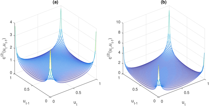
Figure 1: Bivariate marginal copula densities $c^{(2)}(u_{t},u_{t-1}|\bm{\psi})$ of two copulas constructed by inversion of latent nonlinear state space models. Panel (a) is for a first order stochastic volatility model. Here, the values of overall ‘level’ dependence (ie. Kendall’s tau or Spearman’s rho) for this copula are exactly zero, yet the copula has high (equally-valued) tail dependence in all four quadrants. Panel (b) is for a Markov switching autoregression. Here, dependence is asymmetric and quantile dependence differs in each of the four quadrants.

We label the inversion copula constructed from the SVUC model as ‘InvCop1’. Appendix B outlines how to compute the marginal copula density $c^{(2)}(u_{t},u_{t-1}|\bm{\psi})$ for this copula. Because the time series has Markov order one, this bivariate copula characterizes the full serial dependence structure. For example, Figure 1(a) plots $c^{(2)}$ for the case when there is no unobserved mean component (ie. $\rho_{\mu}=\sigma^{2}_{\mu}=0$), $\rho_{\zeta}=0.952$ and $\sigma_{\zeta}=0.045$— typical values arising when fitting asset return data. The copula density is far from uniform, with high equally-valued quantile dependence in all four quadrants ($\lambda^{++}_{1}(0.1)=0.1428,\lambda^{++}_{1}(0.05)=0.0964$ and $\lambda^{++}_{1}(0.01)=0.0454$). This is a high level of first order serial dependence, yet $\tau_{1}=r_{1}=0$. This is because $\tau_{1}$ and $r_{1}$ measure ‘level’ dependence, whereas this copula instead captures bivariate dependence in the second moment. Most existing parametric copulas are not well-suited to represent such serial dependence; see Loaiza-Maya et al. (2016) for a discussion.

We employ the prior $\pi_{\psi}(\bm{\psi})\propto\frac{1}{\sigma^{2}_{\mu}\sigma^{2}_{\zeta}}I(\bm{\psi}\in R_{\psi})$, where $R_{\psi}$ is the region of feasible parameter values conforming to the restrictions listed above, and $I(X)=1$ if $X$ is true, and zero otherwise. We outline here how to implement the Step 1 of the sampling scheme in Section 2.3. We partition the state vector into $\bm{\mu}=(\mu_{1},\ldots,\mu_{T})$ and $\bm{\zeta}=(\zeta_{1},\ldots,\zeta_{T})$, and use the two separate steps:

• Step 1a. Generate from $f(\bm{\mu}|\bm{\psi},\bm{\zeta},\bm{\theta},\bm{y})\propto\prod_{t=1}^{T}\phi_{1}\left(z_{t};\mu_{t};\exp(\zeta_{t})\right)f(\bm{\mu}|\bm{\psi})$

• Step 1b. Generate from $f(\bm{\zeta}|\bm{\psi},\bm{\mu},\bm{\theta},\bm{y})\propto\prod_{t=1}^{T}\phi_{1}\left(z_{t};\mu_{t};\exp(\zeta_{t})\right)f(\bm{\zeta}|\bm{\psi})$

The posterior of $\bm{\mu}$ in Step 1a can be recognized as normal with zero mean and a band 1 precision matrix, so that generation is both straightforward and fast. There are a number of efficient methods to generate $\bm{\zeta}$ in Step 1b in the literature, and we employ the ‘precision sampler’ for the latent states outlined in Chan & Hsiao (2014). This is a fast sparse matrix implementation of the auxiliary mixture sampler (Kim, Shepherd & Chib 1998) that is known to mix well for the stochastic volatility model.

3.2 Markov Switching Inversion Copula

Another popular class of nonlinear state space models are regime switching models, which allow for structural changes in the dynamics of a series. In these models latent regime indicators usually follow an ergodic Markov chain, in which case the model is called a Markov switching model; see Hamilton (1994; Ch.22) for an introduction.

We consider a two regime Markov switching first order autoregressive model (MSAR1) given by

$$Z_{t}|\bm{X}_{t}=\bm{x}_{t}\sim N(c_{s_{t}}+\rho_{s_{t}}z_{t-1},\sigma^{2}_{s_{t}})$$

$$\mbox{Pr}(s_{t}=j|s_{t-1}=i)=p_{ij},$$ (3.2)

for regimes $s_{t}\in\{1,2\}$. This is a nonlinear state space model with state vector $\bm{x}_{t}=\left(z_{t-1},s_{t}\right)$. We assume the Markov chain is ergodic, so that the marginal distribution of $s_{t}$ is time invariant with $\mbox{Pr}(s_{t}=1)=\pi_{1}=(1-p_{22})/(2-p_{11}-p_{22})$ and $\mbox{Pr}(s_{t}=2)=\pi_{2}=1-\pi_{1}$. Denoting $s_{i}^{2}=\sigma_{i}^{2}/(1-\rho_{i}^{2})$, it can be shown that stationarity results from the constraints $|\rho_{j}|<1$ for $j=1,2$, and $s_{i}^{2}s_{j}^{2}-\rho_{j}^{2}(s_{i}^{2})^{2}>0$ for $(i,j)=(1,2),(2,1)$. These provide inequality constraints on each element of $\{\rho_{1},\rho_{2},\sigma^{2}_{1},\sigma^{2}_{2}\}$, given values for the other elements. Following standard practice we identify the two components by assuming $\pi_{1}<\pi_{2}$.

When forming the copula, we assume the marginal mean $E(Z_{t})=\bar{\mu}=\sum_{i=1,2}\pi_{i}\frac{c_{i}}{1-\rho_{i}}=0$ and variance $\mbox{Var}(Z_{t})=\sum_{i=1,2}\pi_{i}\frac{\sigma^{2}_{i}}{1-\rho^{2}_{i}}=1$. This provides the additional equality constraints

$$c_{1} = -\frac{\pi_{2}c_{2}(1-\rho_{1})}{\pi_{1}(1-\rho_{2})}\,,$$

$$\sigma^{2}_{1} = \frac{(1-\rho_{1}^{2})}{\pi_{1}}\left(1-\pi_{2}s^{2}_{2}\right)\,.$$

Also, because $\sigma^{2}_{1}>0$, from the last equality constraint above it follows that $\pi_{2}s^{2}_{2}<1$, which can be satisfied by imposing an upper bound on $p_{22}$. The inversion copula parameters are therefore $\bm{\psi}=\{c_{2},\rho_{1},\rho_{2},\sigma_{2}^{2},p_{11},p_{22}\}$, subject to the inequality constraints above.

The marginal distribution of $Z_{t}$ is a mixture of two Gaussians, with

$$f_{Z_{1}}(z|\bm{\psi})=\sum_{i=1,2}\phi_{1}\left(z;\mu_{i},s_{i}^{2}\right)\pi_{i},$$ (3.3)

where $\mu_{i}=\frac{c_{i}}{1-\rho_{i}}$. Both $f_{Z_{1}}$ and $F_{Z_{1}}$ are therefore fast to compute, and the quantile function $F_{Z_{1}}^{-1}$ is computed using the spline interpolation method outlined in Appendix A. The marginal copula $c^{(2)}$ is given in Appendix B, and is the inversion copula of a mixture of four bivariate Gaussians. This is very different than the more common ‘mixture copula’, which is a finite mixture of copulas; for example, see Patton (2006).

We label the inversion copula constructed from the MSAR1 model as ‘InvCop2’. Unlike the other two inversion copulas examined, it can exhibit asymmetric first order serial dependence. To illustrate, Figure 1(b) plots the marginal copula $c^{(2)}$ when $p_{11}=0.92$, $p_{22}=0.95$, $\sigma^{2}_{2}=0.6$, $\rho_{1}=-0.5$, $\rho_{2}=0.6$ and $c_{2}=0.02$. In this case, $r_{1}=0.159$, $\tau_{1}=0.113$, and quantile dependence is different in each quadrant with $\lambda^{--}_{1}(0.1)=0.249$, $\lambda^{++}_{1}(0.1)=0.201$, $\lambda^{+-}_{1}(0.1)=0.141$ and $\lambda^{-+}_{1}(0.1)=0.144$.

As before, we employ the MCMC algorithm in Section 2.3 to estimate the model. The prior $\pi_{\psi}(\psi)\propto\frac{1}{\sigma^{2}_{2}}I(\bm{\psi}\in R_{\psi})$, where $R_{\psi}$ is the region of feasible parameter values outlined above. A forward filtering and backward sampling algorithm (Hamilton 1994, p.694) is used to sample the regime indicators $\bm{s}=(s_{1},...,s_{T})$ in Step 1.

3.3 Gaussian Unobserved Component Inversion Copula

We also construct an inversion copula from a Gaussian unobserved component model, where the component follows a stationary order $p$ autoregression, so that

$$Z_{t}|\bm{X}_{t}=\bm{x}_{t} \sim N(\mu_{t},\sigma^{2})$$

$$\mu_{t} = \bar{\mu}+\sum_{j=1}^{p}\rho_{j}(\mu_{t-j}-\bar{\mu})+\sigma^{2}_{\mu}\,.$$ (3.4)

This model (labeled here as UCAR$p$) can be written in state space form at Equation (2.7) with state vector $\bm{x}_{t}=(\mu_{t},\mu_{t-1},\ldots,\mu_{t-p+1})$ and appropriate choices for matrices $\bm{b},R,F$ and $Q$. The resulting inversion copula is a Gaussian copula with the specific time series dependence structure, and is labeled ‘InvCop3’.

We follow Barndorff-Neilsen & Schou (1973) and others, and re-parametrize the autoregressive coefficients by the partial correlations $\bm{\pi}=(\pi_{1},\pi_{2},\ldots,\pi_{p})$ via the Durbin-Levinson algorithm. An advantage is that stationarity is easily imposed by the inequalities $|\pi_{j}|<1$ for $j=1,\ldots,p$. When forming the copula, the marginal mean $E(Z_{t})=\bar{\mu}=0$. A second equality constraint $\sigma^{2}=1-\mbox{Var}(\mu_{t})$, where $\mbox{Var}(\mu_{t})=\sigma^{2}_{\mu}\prod_{j=1}^{p}(1-\pi_{j}^{2})^{-1}$, ensures the marginal variance is unity. The parameters of this copula are therefore $\bm{\psi}=\{\bm{\pi},\sigma^{2}_{\mu}\}$, and the prior is $\pi_{\psi}(\bm{\psi})\propto\frac{1}{\sigma^{2}_{\mu}}I(|\pi_{j}|<1)$.

As in Section 3.1, we use the precision sampler to sample the latent states $(\mu_{1},\ldots,\mu_{T})$ at Step 1. In Step 2 of the scheme, the partial correlations $\bm{\pi}$ are sampled jointly using Metropolis-Hasting with a multivariate normal approximation proposal computed as described in Section 2.3, and truncated to the unit cube. The parameter $\sigma_{\mu}^{2}$ is also generated using a truncated normal approximation as a proposal. We show these are adequate proposals in our empirical work.

4 Empirical Analysis

The three inversion copulas in Section 3 are used to model quarterly U.S. broad inflation and U.S. electricity inflation. Here we illustrate that the inversion copulas produce more accurate forecast densities than the three state space models themselves. In the Supplementary Appendix (Part A) we include a simulation study that shows that even the simplest of our proposed inversion copulas with a flexible margin can greatly increase forecast accuracy.

4.1 Modeling and Forecasting U.S. Broad Inflation

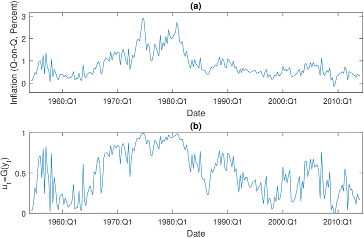
Figure 2: Panel (a) is a time series plot of the quarter-on-quarter U.S. broad inflation data. Panel (b) is a time series plot of the copula data $u_{t}=G(y_{t})$, where $G$ is the distribution function computed from the KDE in Figure 3(a,b).

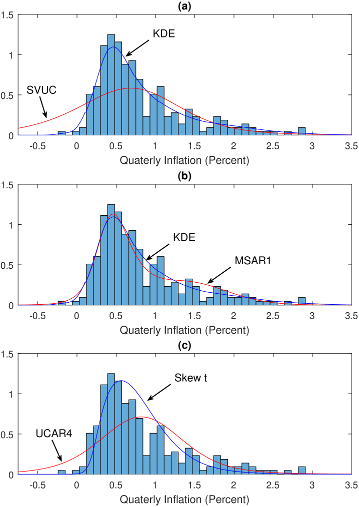
Figure 3: Each panel plots the (normalized) histogram of the U.S. broad inflation data, along with the marginal distributions of the six time series models. Each panel plots the margin used for each of the three copula models in blue, along with the margin arising from the corresponding state space model fit to the same data in red.

We employ our methodology to model and forecast U.S. inflation from 1954:Q1 to 2013:Q4. Inflation is measured by the difference $y_{t}=\log(P_{t})-\log(P_{t-1})$ in the logarithm of the (seasonally adjusted) quarterly GDP price deflator $P_{t}$, sourced from the FRED database of the Federal Reserve Bank of Saint Louis. Figure 2(a) plots the time series of the $T=240$ quarterly observations, while Figure 3 plots histograms of the data. The marginal distribution of inflation is far from symmetric, with sample skew 1.329 and kurtosis 4.515, and a Shapiro & Wilk (1965) test for normality is rejected at any meaningful significance level. A wide range of time series models have been fitted to quarterly inflation data previously (Faust & Wright 2013; Clark & Ravazzolo 2015), including the three state space models considered here. However, these three models— in fact, most time series models used previously— have margins that are inconsistent with that observed empirically. We show that combining each of the three inversion copulas with more flexible margins solves this problem, and significantly improves the accuracy of the one-quarter-ahead predictive densities.

4.1.1 SVUC and InvCop1

Stock & Watson (2007) suggest using an unobserved component model with stochastic volatility for U.S. inflation, and it has become a popular model for this series (Clark & Ravazzolo 2015; Chan 2015). We fit the SVUC model directly to the inflation data using Bayesian methods. Table 2 reports the parameter estimates, labeled as model ‘S1’. (Note that this table also reports the parameter estimates for all five other models fit to this data.) The marginal density for inflation implied by the SVUC model is shown in Figure 3(a) in red. It is necessarily symmetric and inconsistent with that observed empirically.

We therefore employ a copula time series model (labeled ‘C1’) with copula function InvCop1 and a nonparametric margin, for which we employ the kernel density estimator (KDE), with the locally adaptive bandwidth method of Shimazaki & Shinomoto (2010). This copula model allows for the same serial dependence structure as the SVUC model, but with a more accurate margin. The estimated margin is a smooth asymmetric and heavy-tailed distribution, and is also plotted in Figure 3(a). Using this for $g$, the copula data $u_{t}=G(y_{t})$ are computed and plotted in Figure 2(b). This time series retains the serial dependence apparent in the original data.

The copula parameters are estimated using the MCMC scheme, where the proposals in Step 2 of the sampler have acceptance rates between 35% and 41%. There is strong positive correlation in both the level ($\hat{\rho}_{\mu}=0.959$) and the log-volatilities ($\hat{\rho}_{\zeta}=0.789$) of $Z_{t}$, similar to that for the SVUC model fit directly to the inflation data.

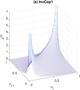
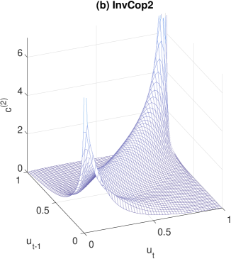
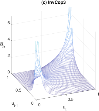
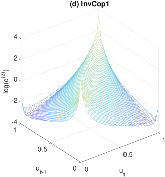
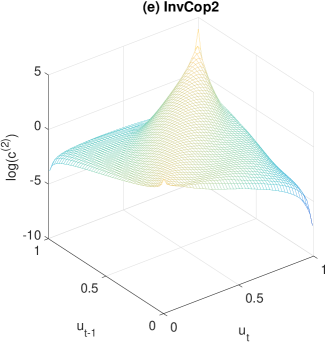
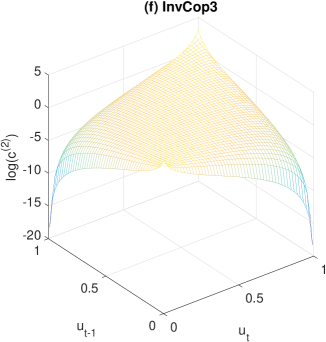
Figure 4: Marginal copula densities $c^{(2)}(u_{t},u_{t-1}|\hat{\bm{\psi}})$ for each of the three inversion copula models fitted to the U.S. broad inflation data. Panels (a,b,c) plot the densities with a common vertical axis truncated at 7 for interpretation. Panels (d,e,f) plot the logarithm of the same three densities. Each density has been computed at the posterior mean $\hat{\bm{\psi}}$ of the copula parameters.

Figure 4(a) plots the marginal copula density $c^{(2)}(u_{t},u_{t-1}|\hat{\bm{\psi}})$ at the parameter estimates. There are spikes in the density close to (0,0) and (1,1), so that the vertical axis is truncated at 7 to aid interpretation. The logarithm of the density is also plotted in panel (d). The majority of mass is along the axis between (0,0) to (1,1), which is due to level dependence captured by the unobserved component. However, the conditional heteroskedasticity also affects the form of the copula, with mass around points (0,1) and (1,0) and four edges apparent in panel (d). Table 3 reports measures of first order serial dependence in $\{Y_{t}\}$ captured by InvCop1. The unobserved mean component results in strong positive overall dependence, with $\hat{r}_{1}=0.792$. There is high (symmetric) quantile dependence $\hat{\lambda}_{1}^{++}(0.05)=\hat{\lambda}^{--}_{1}(0.05)=0.507$, consistent with the shape of $c^{(2)}$.

4.1.2 MSAR1 & InvCop2

Amisano & Fagan (2013) employ the MSAR1 model for U.S. inflation, but only allow $c_{1}$ and $c_{2}$ to vary between regimes. We extend this study here by fitting the more general MSAR1 model (labeled ‘S2’) directly to the inflation data using Bayesian methods. The implied marginal density is shown in Figure 3(b) in red, and it is more consistent with the data than the margin of the SVUC model.

A time series copula model, with margin $G$ given by the KDE and copula function InvCop2, is also fit and labeled as model ‘C2’. The copula parameters are estimated using the MCMC scheme, and the proposals in Step 2 of the sampler have acceptance rates between 13% and 38%. Parameter estimates for both models S2 and C2 show positive serial dependence and high values for $p_{11}$ and $p_{22}$. However, the characteristics of the regimes differ between the two models, and it is shown later that the two models also have very different predictive distributions

Table 3 reports the first order serial dependence metrics of copula InvCop2. Similar to the other copulas, there is high overall dependence with $\hat{r}_{1}=0.752$, although dependence is highly asymmetric with $\hat{\lambda}^{++}_{1}(0.05)=0.644>\hat{\lambda}^{--}_{1}(0.05)=0.272$. This asymmetry is visible in $c^{(2)}$ and $\log(c^{(2)})$, which are plotted in Figure 4(b,e). In contrast, the copulas InvCop1 and InvCop3 do not allow for such asymmetric quantile dependence.

4.1.3 UCAR4 and InvCop3

As a benchmark, the UCAR model with $p=4$ is also fitted, and labeled as model ‘S3’. The margin implied by this model is Gaussian, and plotted in Figure 3(c) in red. The estimates of the partial correlations $\bm{\pi}$ suggest that the unobserved component is Markov order one, which is consistent with the GDP data being seasonally-adjusted. To compare, we also fit a time series copula model (labeled ‘C3’) with copula function InvCop3 and $p=4$. To illustrate estimation of a parametric margin, $G$ is a skew t distribution (Azzalini & Capitanio 2003). The location ($\xi$), scale ($\omega$), skew ($\gamma_{1}$) and kurtosis ($\gamma_{2}$) coefficients are used as parameters, so that $\bm{\theta}=(\xi,\omega,\gamma_{1},\gamma_{2})$. The joint parameter posterior is computed using the MCMC scheme, where $\bm{\theta}$ is generated in Step 3 of the sampler using an adaptive random walk proposal.

Table 2 reports the posterior estimates of both $\bm{\psi}$ and $\bm{\theta}$. The skew t margin has high positive skew $\hat{\gamma}_{1}=1.565$ and heavy tails $\hat{\gamma}_{2}=7.89$, similar to the KDE. In contrast to model S3, the posterior of $\bm{\pi}$ for model C3 suggests that the unobserved component is Markov order two. Figure 4(c,f) plots $c^{(2)}$ and $\log(c^{(2)})$ for InvCop3. This is a bivariate Gaussian copula, and is therefore symmetric along the axes (0,1) to (1,0). As with the other copula functions, overall first order serial dependence is positive with $\hat{r}_{1}=0.789$. Quantile dependence is symmetric and positive for $\alpha>0$, although $\lim_{\alpha\rightarrow 0}\lambda_{1}^{++}(\alpha)=0$ for any Gaussian copula.

4.1.4 Density Forecast Comparison

One-quarter-ahead predictive densities are computed for quarters $t=2,\ldots,T$ for all six fitted models. Point forecast accuracy is measured using the root mean squared error (RMSE). Density forecast accuracy is measured using the (negative) logarithm of the predictive score (LP), the cumulative rank probability score (CRPS) and the tail-weighted CRPS (TW-CRPS). The latter two measures are introduced in Gneiting & Raftery (2007) and Gneiting and Ranjan (2011), and computed directly from the quantile score as in Smith & Vahey (2016). The mean values of the metrics are reported in Table 4, where lower values for all metrics indicate increased accuracy. The density forecasts from the copula models C1, C2 and C3 are all more accurate than those from the corresponding state space models S1, S2 and S3, as measured by mean LP, CRPS and TW-CRPS. However, adopting a copula model results in less of an improvement in RMSE.

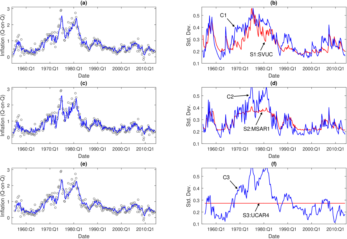
Figure 5: Moments of the one-step-ahead predicitve distributions of the U.S. broad inflation data. Panels (a,c,e) plot in blue the predictive means from each of the three copula models C1, C2 and C3, respectively (See Table 4 for their specification). Also plotted is a scatterplot of the data. Panels (b,d,f) plot the standard deviations of the predictive distributions from the three copula models in blue. The standard deviations of the predictive distributions from the three corresponding state space models, fit directly to the same data, are plotted in red.

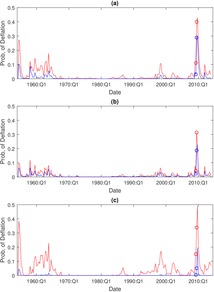
Figure 6: The one-step-ahead predictive probability of deflation from each of the six models fit to the U.S. broad inflation data. The probabilities arising from the copula models are in blue, and the state space models fit directly to the data in red. Panel (a) plots these for models C1 and S1; panel (b) for models C2 and S2; and panel (c) for models C3 and S3. Circles denote the two quarters where (very mild) deflation is recorded in our data (-0.167% during 2009:Q1, and -0.022% during 2009:Q2).

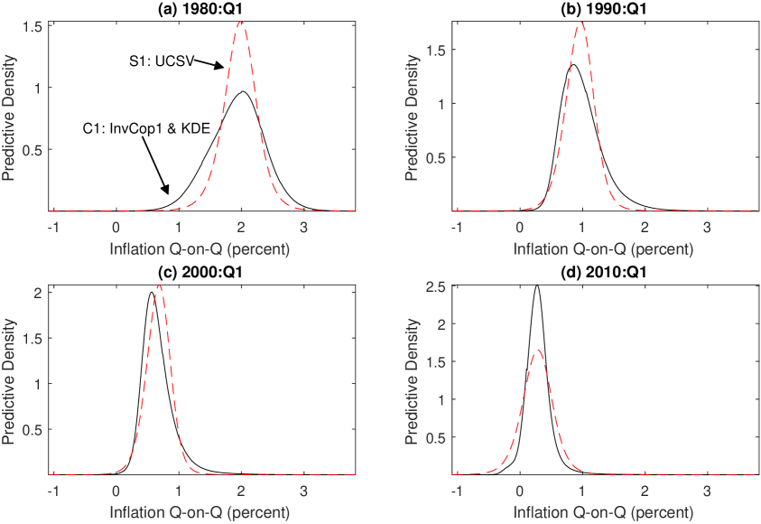
Figure 7: One-quarter-ahead predictive densities of U.S. broad inflation from the UCSV state space model fit directly to the data (S1; red dashed line), and for the copula time series model with copula InvCop1 and KDE margins (C1; black solid line). Results are presented for four quarters: (a) 1980:Q1, (b) 1990:Q1, (c) 2000:Q1, (d) 2010:Q1. Note that the densities from C1 exhibit different skew and kurtosis.

To show how the predictive distributions differ, Figure 5(b,d,f) plots their standard deviation for models C1–C3 in blue, and for models S1–S3 in red; the differences are striking. This is particularly the case for model C3 in panel (f), where the combination of an asymmetric margin with InvCop3 produces heteroskedasticity in the predictive distributions, even though the latent state space model is homoskedastic. A similar feature was observed by Smith & Vahey (2016) when they fit a Gaussian copula. The tails of the predictive distributions also differ. For example, Figure 6 plots the predictive probability of deflation for all models. Broad-based deflation is very rare, with only very mild deflation occurring twice in our data. Yet, the state space models can over-estimate this probability. This is because the inaccuracy of the left hand tails of the margins of models S1–S3 apparent in Figure 3 also extends to the predictive distributions. Figure 7 plots the predictive distributions from models S1 and C1 for four different quarters. It shows that the predictive distributions from the copula model do not simply replicate the asymmetry (or other features) of the marginal distribution. Overall, the best performing model is C1, and its inclusion in a real time forecasting study – such as those by Clark & Ravazzolo (2015) and Smith & Vahey (2016) – is merited.

4.1.5 Computation Times

The MCMC estimation algorithms were implemented in MATLAB using a standard workstation, and computation times varied across the three copula models. The time to complete 1000 sweeps was 667s, 44s and 94s for models C1, C2 and C3, respectively. The greater computing time for model C1 is because $F_{Z_{1}}$ requires evaluation of a univariate numerical integral, as noted in Section 3.1. In addition, model C3 also involves generation of the parameters of the skew t margin. Our empirical results are based on Monte Carlo samples of size 20,000, 25,000 and 30,000 iterates for models C1, C2 and C3, respectively, with a further 5,000, 15,000 and 20,000 iterates discarded for convergence. While we generated more iterates for the faster schemes, we found that varying these did not affect the results meaningfully.

4.1.6 Maximum Likelihood Estimates

We report maximum likelihood estimates of the copula parameters for the U.S. broad inflation example in Table 5 to show that it is possible to estimate the inversion copulas via MLE. All parameter estimates are obtained using two-stage estimation (Joe 2005), where the margin $G$ is first estimated and the copula data $u_{t}=G(y_{t})$ computed for $t=1,\ldots,T$. Conditional upon this copula data, $\bm{\psi}$ is estimated by maximizing the copula density in Equation (2.3). The denominator of this density, as well as the values of $\bm{z}$, are computed from $f_{Z_{1}}$, $F_{Z_{1}}$ and $F_{Z_{1}}^{-1}$ in the same manner as outlined in the paper. The numerator $f_{Z}$ of the copula density can be evaluated for each of our three inversion copulas by filtering algorithms. For InvCop1, the likelihood of the latent SVUC model is computed by the bootstrap particle filter (Gordon et al. 1993), in combination with the Kalman filter. For InvCop2, the likelihood of the latent MSAR1 model is evaluated in closed form using the Hamilton filter for discrete states (see Hamilton 1989). For InvCop3, the likelihood of the latent state space model is Gaussian with moments that can be computed using the Kalman filter. In all cases, $\bm{\psi}$ is constrained as discussed in Section 3, and maximization employs constrained optimization as implemented in the Matlab toolbox. The maximum likelihood estimates reported in Table 5 are in line with the posteriors in Table 2.

4.2 Modeling and Forecasting U.S. Electricity Inflation

To confirm that our methodology applies to other data, we consider inflation in U.S. electricity prices between 1952:Q1 and 2015:Q4 as a second empirical example. The data are differences in the logarithm of the (seasonally-adjusted) quarterly electricity consumer price index of all urban consumers. This series is produced by the U.S. Bureau of Labor Statistics, and available from the FRED database. The time series plots of the $T=256$ observations of the data and the associated copula data are given in Figure 1 of the Supplementary Appendix. The marginal distribution of the data is highly non-Gaussian, and we fit the same six models to this item-specific inflation data, as we do the broad inflation measure in Section 4.1. Even though the data differ, the three state space models S1, S2 and S3 remain attractive time series models for item-specific inflation.

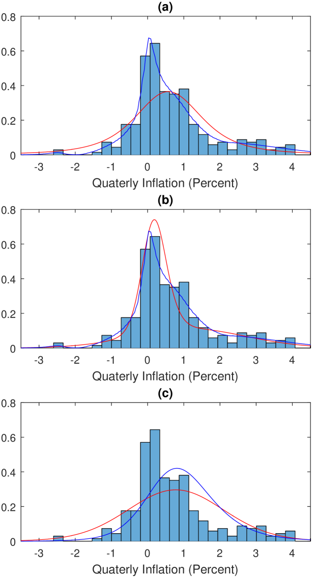
Figure 8: Each panel plots the (normalized) histogram of the U.S. electricity inflation data, along with the marginal distributions of the six time series models. Each panel plots the margin used for each of the three copula models in blue, along with the margin arising from the corresponding state space model fit to the same data in red.

Figure 8 plots the histogram of the data in every panel. As with the broader inflation measure, electricity inflation is positively skewed. It also exhibits an excentuated peak around 0%. The marginal distributions of the fitted state space models S1, S2 and S3 are plotted in red in panels (a,b,c), respectively. The symmetric margins of S1 (the SVUC model) and S3 (the UCAR4 model) are highly inconsistent with the data. Also plotted in blue in panels (a,b) is the adaptive KDE estimate — which is far from symmetric — as is the margin of both copula models C1 and C2. Panel (c) plots the posterior estimate of the skew t distribution, which is the margin of copula model C3. It is positively skewed and heavy-tailed. In each case, the margins of the copula models are more accurate than those implied by the respective state space models.

The copula densities from all three models are similar to those in the broad inflation case, with the bivariate marginal copulas $c^{(2)}(u_{t},u_{t-1})$ showing strong positive dependence (see Figure 2 of the Supplementary Appendix). This is unsurprising because electricity consumption is a major component of economic output. As in Section 4.1, we compute the one-quarter-ahead predictive distributions for all six models at times $t=2,\ldots,T$. Table 6 reports the accuracy metrics, and in each case the copula time series models out-perform their equivalent state space models using every metric. One-sided t-tests of the CRPS and log-score suggest that these differences are statistically significant. As with the analysis of broad inflation, the flexible modelling of the highly asymmetric margin increases the quality of the fitted time series model and the accuracy of these predictive densities. Illustration of the stark differences between the one-quarter-ahead predictive densities from the state space models, and their equivalent copula models, is given in Figure 3 of the Supplementary Appendix.

5 Discussion

This paper proposes a new class of copulas for capturing serial dependence. They are constructed from inversion of a general nonlinear state space model, so that the potential range of dependence structures that they can produce is incredibly broad. A major insight is that such copulas can be very different than those that are widely used for capturing cross-sectional dependence. The latter include elliptical and vine copulas, which have also been used previously to capture serial dependence; see Joe (1997), Beare (2010), Smith et al. (2010) and Loaiza-Maya et al. (2017) for examples. Yet, the three inversion copulas studied in detail highlight the wider serial dependence structures that can be captured by our approach.

As with the likelihood of the underlying state space model, in general the density of the inversion copula cannot be expressed in closed form. However, an important insight is that existing methods for evaluating the likelihood of the latent state space model can also be employed in the copula context. While we employ MCMC samplers to evaluate the posterior, other existing methods can also be used to compute the numerator of the copula density, as we do in Section 4.1.6. Either way, a major computational challenge is the repeated evaluation of the quantile $F_{Z_{t}}^{-1}$ and density $f_{Z_{t}}$ functions at the $T$ observations. When the latent state space model is stationary, we show how this can be achieved using spline approximations to $F_{Z_{1}}^{-1}$ and $\log(f_{Z_{1}})$ outlined in Appendix A. These approximations are highly accurate in our examples, fast to derive, and can be employed with even very large values of $T$ in practice.

Recently, Oh & Patton (2015) construct an inversion copula from a flexible parametric distribution formed through marginalization over a low-dimensional vector of latent factors. This latent factor model can be written in state space form, where the factors are a static state vector $\bm{X}_{t}$ that does not vary with $t$ at Equation (2.5). Full likelihood-based estimation can then be undertaken using the Bayesian MCMC methods discussed here, providing a better alternative to the moment-based method suggested by Oh & Patton (2015). While these factor copulas are unsuitable for serial dependence, Oh & Patton (2015) show they can capture high-dimensional cross-sectional dependence well.

An interesting result is that the inversion copula of a Gaussian linear state space model is a Gaussian copula. Therefore, in this special case, the likelihood is available in closed form. Nevertheless, estimation using simulation methods can still prove efficient, just as it is for the latent state space model itself. While all three of our example inversion copulas are Markov and stationary, copulas can also be derived from non-stationary latent state space models. The resulting time series copula model is also non-stationary, but with a time invariant margin. Such copula models are an interesting topic for further study, although a new approach to computing $F_{Z_{t}}^{-1}$ and $f_{Z_{t}}$ efficiently is needed. A second interesting extension is to employ the proposed time series inversion copulas to capture serial dependence in discrete data. Here, the copula remains unchanged, but $G$ would be a discrete distribution function. The model can be estimated using Bayesian data augmentation, as discussed in Pitt, Chan & Kohn (2006) and Smith, Gan & Kohn (2012). This would require $\bm{z}$ to be generated as an additional step in the sampling scheme in Section 2.3.

A third highly useful extension is to construct the inversion copula of a multivariate state space model. If the dimension of the multivariate time series is $m$, then the resulting $Tm$-dimensional copula captures both cross-sectional and serial dependence jointly. This would provide an alternative to the vine copula models of Smith (2015), Beare & Seo (2015) and Loaiza-Maya et al. (2017) for this case. While the extension is straightforward in principle, implementation relies on the ability to evaluate the univariate marginal distribution functions (and their inverses) for each series of the latent state space model.

To show our methodology can improve the quality of forecast densities, we use it to model and forecast quarterly U.S. broad inflation and U.S. electricity inflation, which is an important problem in empirical macroeconomics (Faust & Wright 2013). We employ inversion copulas constructed from three state space models used previously for this series. When combined with highly asymmetric and heavy-tailed nonparametric or flexible marginal distributions, the predictive distributions from the resulting copula time series models are more accurate than those of the state space models themselves. This is because these state space models have rigid margins, which are very far from that observed for inflation empirically— a problem resolved by the copula models.

Acknowledgments
The work of Michael Smith was supported by Australian Research Council Grant FT110100729.

Appendix

Part A: Fast Evaluation of the Marginal Density and Quantile Function
This part of the appendix outlines how to efficiently evaluate the quantile function $F_{Z_{1}}^{-1}$ and the logarithm of the marginal density $\log(f_{Z_{1}}(z))$ for a stationary nonlinear state space model. For both, we use spline interpolations based on their values at $N$ absciassae, where we set $N=100$ in practise. The advantage of such spline-based approximations is that they are highly accurate (between 5 and 9 decimal places in our empirical work), yet are fast to compute at the $T$ observations once the interpolation is complete– even for large values of $T$.

We use a uniform grid for the $N$ quantile function values $\{q_{1},\ldots,q_{N}\}$, which have correpsonding probability values $\{p_{1},\ldots,p_{N}\}$. We set $p_{1}=0.0001$ and $p_{N}=0.9999$, so that the function is approximated far into the tails of the distribution. The following steps obtain the points at which the interpolations are made.

• Set $p_{1}=0.0001$ and $p_{N}=0.9999$, and evaluate both $q_{1}=F_{Z_{1}}^{-1}(p_{1})$ and $q_{N}=F_{Z_{1}}^{-1}(p_{N})$ using a root finding algorithm.

• Set step size to $\delta=(q_{N}-q_{1})/(N-1)$, and a construct uniform grid as $q_{i}=q_{1}+(i-1)\delta$, for $i=2,\ldots,N$.

• For $i=1,\ldots,N$ (in parallel):
  3a. Compute $p_{i}=F_{Z_{1}}(q_{i})$
  3b. Compute $b_{i}=\log(f_{Z_{1}}(q_{i}))$

We then interpolate the points $\{(p_{i},q_{i});i=1,\ldots,N\}$ and $\{(q_{i},b_{i});i=1,\ldots,N\}$ using splines. We employ natural cubic smoothing splines using the (fast and efficient) spline toolbox in MATLAB, although other fast interpolating methods could also be employed. Notice that numerical inversion of $F_{Z_{1}}$ is undertaken above only twice in Step 1. Moreover, $F_{Z_{1}}$ and $f_{Z_{1}}$ are evaluated only $N$ times in step 3, something that can also be undertaken parallel.

Once the coefficients of the splines are obtained, the log-density and quantile function can be evaluated quickly at even very large number of points $\{z_{1},\ldots,z_{n}\}$. If $F_{Z_{1}}$ is also symmetric (as in Section 3.1), then $F_{Z_{1}}^{-1}(1-u)=-F_{Z_{1}}^{-1}(u)$ for $0\leq u\leq 1/2$, $f_{Z_{1}}(z)=f_{Z_{1}}(-z)$ and $F_{Z_{1}}(-z)=1-F_{Z_{1}}(z)$ for $z\geq 0$. These identities can be exploited to reduce the number of computations at Steps 1 and 3 by one half, further speeding the algorithm.

To illustrate the effectiveness of the method, we consider the approximations to $F_{Z_{1}}^{-1}$ and $\log(f_{Z_{1}})$ for InvCop1 when $\bm{\psi}$ equals the posterior mean in the inflation study in Section 4.1.1. Plots of the approximations (see Figure 4 of the supplementary material) are visually indistinguishable from the true functions, which can be evaluated (slowly) using numerical methods. The integrated absolute difference between the approximate and true functions are $1.282\times 10^{-6}$ and $2.253\times 10^{-10}$ for the quantile and log-density, respectively, so that the approximations are very accurate. Computation of both approximations, and their evaluation at the $T=240$ observations, takes only 0.29s using MATLAB on a standard four core desktop.

Part B: Bivariate Marginal Copulas
This part of the appendix shows how to evaluate the bivariate marginal copula density

$$c^{(2)}(u_{1},u_{2};\bm{\psi})=\frac{f_{Z}^{(2)}(z_{1},z_{2}|\bm{\psi})}{f_{Z_{1}}(z_{2}|\bm{\psi})f_{Z_{1}}(z_{1}|\bm{\psi})}\,,$$

for InvCop1 and InvCop2. In both cases, the univariate marginal density $f_{1}(z|\bm{\psi})$ can be computed readily as in Part A above. Computation of $f_{Z}^{(2)}$ is outlined separately for each case below.

For InvCop1
For the SVUC model with the parameter constraints, the bivariate density

$$f^{(2)}_{Z}(z_{1},z_{2}|\bm{\psi})=\int\int\int\int\phi_{2}\left(\bm{z};\bm{\mu},V(\bm{\zeta})\right)\,\phi_{2}(\bm{\mu};\bm{0},S_{\mu})\mbox{d}\bm{\mu}\,\phi_{2}(\bm{\zeta};(\bar{\zeta},\bar{\zeta}),S_{\zeta})\mbox{d}\bm{\zeta}\,,$$

where $\bm{z}=(z_{1},z_{2})$, $\bm{\mu}=(\mu_{1},\mu_{2})$, $\bm{\zeta}=(\zeta_{1},\zeta_{2})$,

$$V(\bm{\zeta})=\left[\begin{array}[]{cc}\exp(\zeta_{1})&0\\ 0&\exp(\zeta_{2})\end{array}\right],\,S_{\zeta}=s_{\zeta}^{2}\left[\begin{array}[]{cc}1&\rho_{\zeta}\\ \rho_{\zeta}&1\end{array}\right],\,S_{\mu}=s_{\mu}^{2}\left[\begin{array}[]{cc}1&\rho_{\mu}\\ \rho_{\mu}&1\end{array}\right],\,$$

and $\phi_{2}(\bm{x};\bm{a},\Omega)$ is a bivariate normal density with mean $\bm{a}$ and variance $\Omega$ evaluated at point $\bm{x}$. The inner two integrals in $\bm{\mu}$ of this 4-dimensional integral can be computed analytically by recognising a bivariate normal. Then, by recognising a second bivariate normal in $\bm{z}$, the density can be written as:

$$f(z_{1},z_{2}|\bm{\psi})=\int\int\phi_{2}(\bm{z};\bm{0},W(\bm{\zeta}))\phi_{2}(\bm{\zeta};(\bar{\zeta},\bar{\zeta}),S_{\zeta})\mbox{d}\bm{\zeta}\,,$$

where $W(\bm{\zeta})=(S_{\mu}+V(\bm{\zeta}))$. This bivariate integral can be computed numerically.

For InvCop2
For the MSAR1 model with the parameter constraints, the bivariate density is the mixture of four bivariate Gaussians

$$f^{(2)}_{Z}(z_{1},z_{2}|\bm{\psi})=\sum_{i=1,2}\sum_{j=1,2}\phi_{2}\left((z_{1},z_{2});\bm{\mu}_{ij},S_{ij}\right)p_{ij}\pi_{i}\,,$$

where $\bm{\mu}_{ij}=\left(\mu_{i},\mu_{j}\right)$ and

$$S_{ij}=\begin{bmatrix}s^{2}_{i}&\rho_{j}s^{2}_{i}\\ \rho_{j}s^{2}_{i}&s^{2}_{j}\end{bmatrix}\,.$$

References

• Almeida, C. and C. Czado, (2012). ‘Bayesian inference for stochastic time-varying copula models’, Computational Statistics & Data Analysis, 56, 1511–1527.

• Amisano, G. & G. Fagan, (2013). ‘Money growth and inflation: A regime switching approach’, Journal of International Money and Finance, 33, 118–145.

• Azzalini, A. & A. Capitanio, (2003). ‘Distribution generated by perturbation of symmetry with emphasis on a multivariate skew t distribution’, Journal of the Royal Statistical Society, Series B, 65, 367–389.

• Barndorff-Nielsen, O. & G. Schou, (1973). ‘On the Parameterization of Autoregressive Models by Partial Autocorrelations’, Journal of Multivariate Analysis, 3, 408–419.

• Beare, B. K., (2010). ‘Copulas and temporal dependence’, Econometrica, 78, 395–410.

• Beare, B. K., & J. Seo (2015). ‘Vine copula specifications for stationary multivariate Markov chains’, Journal of Time Series Analysis, 36, 228–246.

• Brockwell, P.J. & R.A. Davis, (1991), Time Series: Theory and Methods, 2nd Ed., NY: Springer.

• Chan, J.C.C (2015). ‘The Stochastic Volatility in Mean Model with Time-Varying Parameters: An Application to Inflation Modeling’, Journal of Business and Economic Statistics, to appear.

• Chan, J.C.C. & C.Y.L. Hsiao, (2014). ‘Estimation of Stochastic Volatility Models with Heavy Tails and Serial Dependence’, in Bayesian Inference in the Social Sciences, Eds. I. Jeliazkov and X.-S. Yang, Wiley: NJ.

• Clark, T. E. & F. Ravazzolo, (2015). ‘Macroeconomic Forecasting Performance under Alternative Specifications of Time-varying Volatility’, Journal of Applied Econometrics, 30, 551–575.

• Creal, D.D. & R.S. Tsay, (2015). ‘High dimensional dynamic stochastic copula models’, Journal of Econometrics, 189, 335–345.

• DeJong, D.N., R. Liesenfeld, G.V. Moura, J.-F. Richard, H. Dharmarajan, (2013). ‘Efficient Likelihood Evaluation of State-Space Representations’, Review of Economic Studies, 30, 538–567.

• De Lira Salvatierra, I. & A.J. Patton (2015), ‘Dynamic copula models and high frequency data’, Journal of Empirical Finance, 30, 120–135.

• Demarta, S. & A. McNeil, (2005). ‘The t-copula and related copulas’, International Statistical Review, 73, 111–129.

• Durbin, J. & S.J. Koopman, (2012). Time Series Analysis by State Space Methods, 2nd Ed., OUP.

• Embrechts, P., A. McNeil & D. Straumann, (2001). ‘Correlation and dependency in risk management: properties and pitfalls’, in M. Dempster & H. Moffatt, (Eds.) Risk Management: Value at Risk and Beyond Cambridge University Press, 176–223.

• Faust, J. & J. Wright, (2013). ‘Forecasting Inflation’, in G. Elliot & A. Timmermann (eds.), Handbooks in Economics, Vol. 2A., 3–56.

• Frees, E.W. & P. Wang, (2006). ‘Copula credibility for aggregate loss models’, Insurance: Mathematics and Economics, 38, 360–373.

• Hafner, C.M. & H. Manner, (2012). ‘Dynamic stochastic copula models: estimation, inference and applications’, Journal of Applied Econometrics, 27, 269–295.

• Hamilton, J.D., (1994). Time Series Analysis, Princeton University Press: NJ.

• Gneiting, T. & A.E. Raftery, (2007). ‘Strictly Proper Scoring Rules, Prediction and Estimation’, Journal of the American Statistical Association, 102, 359–378.

• Gneiting, T. & R. Ranjan, (2011). ‘Comparing Density Forecasts using Threshold- and Quantile-Weighted Scoring Rules’, Journal of Business and Economic Statistics, 29, 411–422.

• Godsill, S., A. Doucet & M. West (2004). ‘Monte Carlo Smoothing for Nonlinear Time Series’, Journal of the American Statsitical Association, 99, 156–168.

• Gordon, N.J., D.J. Salmond and A.F.M. Smith (1993). ‘A Novel Approach to Non-Linear and Non-Gaussian Bayesian State Estimation’, IEEE Proceedings, F140, 107–133.

• Hamilton, J.D. (1989). ‘A New Approach to the Economic Analysis of Nonstationary Time Series and the Business Cycle’, Econometrica, 57, 357–384.

• Joe, H., (1997). Multivariate Models and Dependence Concepts, Chapman and Hall.

• Joe, H. (2005). ‘Asymptotic Efficiency of the Two-Stage Esimation Method for Cupula-Based Models’, Journal of Multivariate Analysis, 94, 401–419.

• Jungbacker, B. & S.J. Koopman (2007). ‘Monte Carlo Estimation for Nonlinear Non-Gaussian State Space Models’, Biometrika, 94: 4, 827-839.

• Kauermann, G., C. Schellhase, D. Ruppert (2013). ‘Flexible Copula Density Estimation with Penalized Hierarchical B-splines’, Scandinavian Journal of Statistics: Theory and Applications, 40, 685–705.

• Kim, S., N. Shephard & S. Chib, (1998). ‘Stochastic Volatility: Likelihood Inference and Comparison with ARCH Models’, Review of Economic Studies, 65, 361–393.

• Lambert, P. & F. Vandenhende, (2002). ‘A copula-based model for multivariate non-normal longitudinal data: analysis of a dose titration safety study on a new antidepressant’, Statistics in Medicine, 21, 3197–3217.

• Ljung, L. (1999). System Identification: Theory for the User, 2nd Ed., Prentice-Hall.

• Loaiza-Maya, R., M.S. Smith & W. Maneesoonthorn (2017). ‘Time Series Copulas for Heteroskedastic Data’, Journal of Applied Econometrics, forthcoming.

• Lütkepohl, H., (2006). New Introduction to Multiple Time Series Analysis, Springer-Verlag: Berlin.

• Oh, D.H. & A.J. Patton (2015). ‘Modelling Dependence in High Dimensions with Factor Copulas’, Journal of Business and Economic Statistics, forthcoming.

• Nelsen, R., (2006), An Introduction to Copulas. 2nd ed., New York, Springer.

• Patton, A.J., (2006). ‘Modelling Asymmetric Exchange Rate Dependence’, International Economic Review, 47, 527–556.

• Patton, A.J., (2012). ‘A Review of Copula Models for Economic Time Series’, Journal of Multivariate Analysis, 110, 4–18.

• Pitt, M., D. Chan & R. Kohn (2006). ‘Efficient Bayesian Inference for Gaussian Copula Regression Models’, Biometrika, 93, 537–554.

• Richard, J.F. & W. Zhang, (2007). ‘Efficient high-dimensional importance sampling’, Journal of Econometrics, 141, 1385–1411.

• Scharth, M. & Kohn, R., (2016). ‘Particle Efficient Importance Sampling’, Journal of Econometrics, 190, 133–147.

• Shapiro, S. & M. Wilk, (1965). ‘An Analysis of Variate Test for Normality (Complete Samples)’, Biometrika, 52, 3-4, 591–611.

• Shephard, N. & M. Pitt, (1997). ‘Likelihood analysis of non-Gaussian measurement time series’, Biometrika, 84:3, 653–667.

• Shih, J.H. & T.A. Louis, (1995). ‘Inferences on the association parameter in copula models for bivariate survival data’, Biometrics, 51, 4, 1384–99.

• Shimazaki, H. & S. Shinomoto, (2010). ‘Kernel bandwidth optimization in spike rate estimation’, Journal of Computational Neuroscience, 29, 171–182.

• Smith, M.S., (2015). ‘Copula modelling of dependence in multivariate time series’, International Journal of Forecasting, 31, 815–833.

• Smith, M.S., Q. Gan & R. Kohn (2012). ‘Modelling Dependence using Skew t Copulas: Bayesian Inference and Applications’, Journal of Applied Econometrics, 27, 500–522.

• Smith, M., A. Min, C. Almeida & C. Czado, (2010). ‘Modeling Longitudinal Data using a Pair-Copula Decomposition of Serial Dependence’, Journal of the American Statistical Association, 105, 492, 1467-1479.

• Smith, M.S. & S.P. Vahey, (2016). ‘Asymmetric density forecasting of U.S. macroeconomic variables using a Gaussian copula model of cross-sectional and serial dependence’, Journal of Business and Economic Statistics, 34:3, 416–434.

• Song, P. (2000). ‘Multivariate Dispersion Models Generated from Gaussian Copula’, Scandinavian Journal of Statistics, 27, 305–320.

• Stock, J.H. and M.W. Watson, (2007). ‘Why Has U.S. Inflation Become Harder to Forecast?’, Journal of Money, Credit and Banking, 39, 3–33.

• Stroud, J.R., P. Müller & N.G. Polson, (2003). ‘Nonlinear State-Space Models with State-Dependence Variances’, Journal of the American Statistical Association, 98:462, 377–386.

• Tsukahara, H. (2005). ‘Semiparametric estimation in copula models’, The Canadian Journal of Statistics, 33, 357–375.

		$U_{t}=G(Y_{t})$		$Z_{t}=F_{Z_{t}}^{-1}(U_{t})$
Process	$\{Y_{t}\}_{t=1}^{T}$	$\longrightarrow$	$\{U_{t}\}_{t=1}^{T}$	$\longrightarrow$	$\{Z_{t}\}_{t=1}^{T}$
Domain	${\cal S}_{Y}\subset{\cal R}^{T}$	$\longrightarrow$	$[0,1]^{T}$	$\longrightarrow$	${\cal S}_{Z}\subset{\cal R}^{T}$
Joint CDF	$F_{Y}(\bm{y})$	$\longrightarrow$	$C(\bm{u})$	$\longrightarrow$	$F_{Z}(\bm{z})$
Marginal CDFs	$G(y_{t})$	$\longrightarrow$	Uniform	$\longrightarrow$	$F_{Z_{t}}(z_{t})$

Table 1: Depiction of the transformations underlying an inversion copula model when $Y_{t}$ is continuous-valued.

Copula Time Series Models
Model C1: InvCop1 & KDE Margin
$\rho_{\mu}$	$\sigma^{2}_{\mu}$	$\rho_{\zeta}$	$\sigma^{2}_{\zeta}$	$\bar{\zeta}$	$\bar{\mu}$
0.959	0.066	0.789	0.603	-2.573	0
(0.94,0.97)	(0.04, 0.10)	(0.48,0.96)	(0.08,1.69)	(-3.26,-1.94)	–
Model C2: InvCop2 & KDE Margin
$c_{1}$	$\rho_{1}$	$\sigma^{2}_{1}$	${s^{2}_{1}}$	$p_{11}$	$\pi_{1}$
$-0.554$	0.207	0.752	0.815	0.865	0.354
(-0.85,-0.33)	(-0.11,0.46)	(0.53,0.98)	(0.57,1.06)	(0.75,0.95)	(0.20,0.46)
$c_{2}$	$\rho_{2}$	$\sigma^{2}_{2}$	${s^{2}_{2}}$	$p_{22}$	$\pi_{2}$
0.040	0.914	0.199	1.239	0.930	0.646
(0.01,0.08)	(0.88,0.94)	(0.16,0.25)	(0.98,1.53)	(0.88,0.97)	(0.54,0.80)
Model C3: InvCop3 & Skew t Margin
$\pi_{1}$	$\pi_{2}$	$\pi_{3}$	$\pi_{4}$	$\sigma^{2}_{\mu}$	$\sigma^{2}$
0.866	0.371	-0.037	0.113	0.181	0.088
(0.81,0.93)	(0.16,0.55)	(-0.41,0.22)	(-0.14,0.31)	(0.08,0.28)	(0.01,0.16)
$\bar{\mu}$	$\xi$	$\omega$	$\gamma_{1}$	$\gamma_{2}$
0	0.202	0.549	1.565	7.890
–	(0.16,0.25)	(0.45,0.66)	(1.54,1.59)	(7.65,8.14)
State Space Models
Model S1: SVUC
$\rho_{\mu}$	$\sigma^{2}_{\mu}$	$\rho_{\zeta}$	$\sigma^{2}_{\zeta}$	$\bar{\zeta}$	$\bar{\mu}$
0.976	0.014	0.904	0.320	-3.896	0.645
(0.95,0.99)	(0.01,0.02)	(0.77,0.98)	(0.07,0.82)	(-4.83,-3.02)	(-0.03,1.22)
Model S2: MSAR1
$c_{1}$	$\rho_{1}$	$\sigma^{2}_{1}$	${s^{2}_{1}}$	$p_{11}$	$\pi_{1}$
0.438	0.687	0.124	0.253	0.960	0.367
(0.19,0.72)	(0.53, 0.83)	(0.09,0.16)	(0.17,0.39)	(0.91,0.99)	(0.18,0.48)
$c_{2}$	$\rho_{2}$	$\sigma^{2}_{2}$	${s^{2}_{2}}$	$p_{22}$	$\pi_{2}$
0.247	0.479	0.039	0.076	0.979	0.633
(0.06,0.35)	(0.19, 0.89)	(0.02,0.06)	(0.02,0.23)	(0.96,0.99)	(0.52,0.82)
Model S3: UCAR4
$\pi_{1}$	$\pi_{2}$	$\pi_{3}$	$\pi_{4}$	$\sigma^{2}_{\mu}$	$\sigma^{2}$
0.920	0.333	-0.152	0.040	0.037	0.023
(0.82,0.98)	(-0.03,0.63)	(-0.63,0.25)	(-0.35,0.30)	(0.01,0.07)	(0.00,0.04)
$\bar{\mu}$
0.859
(0.337,1.387)

Table 2: Posterior parameter estimates for the six models fit to the U.S. broad inflation data. The top half of the table reports estimates for the three inversion copulas constructed from latent state space models. The bottom half reports estimates for the same state space models fit directly to the data. The posterior mean of each parameter is reported, along with 90% posterior probability intervals below. For InvCop3, the parameters of the jointly estimated skew t margin are also reported. The identification constraint $\bar{\mu}=0$ occurs in both InvCop1 and InvCop3.

	Dependence Metric
	$r_{1}$	$\tau_{1}$	$\lambda_{1}^{\tiny--}(0.01)$	$\lambda_{1}^{\tiny--}(0.05)$	$\lambda_{1}^{\tiny++}(0.01)$	$\lambda_{1}^{\tiny++}(0.05)$
Copula
InvCop1	0.792	0.611	0.335	0.507	Sym	Sym
InvCop2	0.752	0.577	0.191	0.272	0.554	0.644
InvCop3	0.789	0.578	0.362	0.482	Sym	Sym

Table 3: Posterior means of first order serial dependence measures for each of the three inversion copulas fit to the U.S. broad inflation data. The copulas InvCop1 and InvCop3 have symmetric tail dependence, while InvCop2 has asymmetric tail dependence.

Model	LP	CRPS	TW-CRPS	RMSE
Copula Time Series Models
C1: KDE Margin & InvCop1	$-0.0266^{\star}$	$0.1393^{\star\star}$	$0.0308^{\star}$	$0.2641^{\star}$
C2: KDE Margin & InvCop2	$-0.0086^{\star\star}$	0.1440	0.0322	0.2746
C3: Skew t Margin & InvCop3	0.0409	$0.1412^{\star}$	$0.0312^{\star\star}$	0.2638
State Space Models
S1: SVUC	0.0166	0.1439	0.0318	0.2712
S2: MSAR1	0.0424	0.1485	0.0330	0.2827
S3: UCAR4	0.0896	0.1445	0.0328	0.2618

Table 4: Summary of the accuracy of the one-step-ahead predictive distributions for the six models fit to the U.S. broad inflation data. The metrics are the mean (negative) logarithm predictive score (LP), the mean cumulative rank probability score (CRPS), the mean tail-weighted CRPS (TW-CRPS), and the root mean squared error (RMSE). Lower values of all metrics indicate improved accuracy. The first three models employ inversion copulas constructed from latent state space models, along with an asymmetric margin. The bottom three are the same state space models fit directly to the data. When the result for a copula model is statistically significantly better than the corresponding state space model, it is indicated with ‘$\star$’ at 10% significance level or ‘$\star\star$’ at 5% significance level.

Model C1: KDE Margin & InvCop1
$\rho_{\mu}$	$\sigma^{2}_{\mu}$	$\rho_{\zeta}$	$\sigma^{2}_{\zeta}$	$\bar{\zeta}$	$\bar{\mu}$
0.948	0.062	0.696	0.567	$-1.495$	0
Model C2: KDE Margin & InvCop2
$c_{1}$	$\rho_{1}$	$\sigma^{2}_{1}$	${s^{2}_{1}}$	$p_{11}$	$\pi_{1}$
$-0.178$	0.338	0.750	0.846	0.832	0.145
$c_{2}$	$\rho_{2}$	$\sigma^{2}_{2}$	${s^{2}_{2}}$	$p_{22}$	$\pi_{2}$
0.004	0.919	0.159	1.025	0.972	0.855
Model C3: Skew t Margin & InvCop3
$\pi_{1}$	$\pi_{2}$	$\pi_{3}$	$\pi_{4}$	$\sigma^{2}_{\mu}$	$\sigma^{2}$
0.954	0.393	$-0.542$	0.276	0.04	0.144
$\bar{\mu}$	$\xi$	$\omega$	$\gamma_{1}$	$\gamma_{2}$
0	0.172	0.569	1.566	7.891

Table 5: Maximum likelihood parameter estimates for the three inversion copulas constructed from latent state space models and fit to the U.S. broad inflation data. For InvCop3, the parameters of the estimated skew t margin are also reported. The identification constraint $\bar{\mu}=0$ occurs in both InvCop1 and InvCop3.

Model	LP	CRPS	RMSE
Copula Time Series Models
C1: KDE Margin & InvCop1	$1.170^{\star\star}$	$0.522^{\star}$	1.058
C2: KDE Margin & InvCop2	$1.197^{\star}$	0.543	1.087
C3: Skew t Margin & InvCop3	$1.382^{\star\star\star}$	$0.561^{\star}$	1.088
State Space Models
S1: SVUC	1.223	0.538	1.090
S2: MSAR1	1.241	0.548	1.097
S3: UCAR4	1.486	0.574	1.077

Table 6: Summary of the accuracy of the one-step-ahead predictive distributions for the six models fit to the U.S. electricity inflation data. The metrics are the mean (negative) logarithm predictive score (LP), the mean cumulative rank probability score (CRPS), and the root mean squared error (RMSE). Lower values for all metrics indicate improved accuracy. The first three models employ inversion copulas constructed from latent state space models, along with an asymmetric margin. The bottom three are the same state space models fit directly to the data. When the result for a copula model is statistically significantly better than the corresponding state space model, it is indicated with ‘$\star$’ at 10% significance level, ‘$\star\star$’ at 5% significance level or ‘$\star\star\star$’ at 1% significance level.