Detection of an oxygen emission line from a high redshift galaxy in the reionization epoch

The physical properties and elemental abundances of the interstellar medium in galaxies during cosmic reionization are important for understanding the role of galaxies in this process. We report the Atacama Large Millimeter/submillimeter Array detection of an oxygen emission line at a wavelength of 88 micrometers from a galaxy at an epoch about 700 million years after the Big Bang. The oxygen abundance of this galaxy is estimated at about one-tenth that of the Sun. The non-detection of far-infrared continuum emission indicates a deficiency of interstellar dust in the galaxy. A carbon emission line at a wavelength of 158 micrometers is also not detected, implying an unusually small amount of neutral gas. These properties might allow ionizing photons to escape into the intergalactic medium.

The physical and chemical conditions of the interstellar medium (ISM) in galaxies can be revealed with forbidden atomic emission lines from the warm-phase ISM, such as ionized hydrogen (H ii) regions and photodissociation regions (PDRs). A far-infrared (FIR) forbidden emission line, the [C ii] 158 $\mu$m line predominantly coming from PDRs, has already been detected in many high-$z$ objects  (?, ?). Recent observations with the Atacama Large Millimeter/submillimeter Array (ALMA) have revealed the [C ii] line emission from young star-forming galaxies emitting a strong hydrogen Ly$\alpha$ line, so-called Ly$\alpha$ emitters (LAEs), at redshift $z\sim 5$ to 6  (?, ?). However, ALMA observations have also shown that LAEs at $z>6$ have at least an order of magnitude lower luminosity of the [C ii] line than that expected from their star formation rate (SFR)  (?, ?, ?, ?), suggesting unusual ISM conditions in these high-$z$ LAEs  (?).

Herschel observations of nearby dwarf galaxies, on the other hand, have revealed that a forbidden oxygen line, [O iii] 88 $\mu$m, is much stronger than the [C ii] line in these chemically unevolved galaxies  (?, ?, ?). The Infrared Space Observatory and the Japanese infrared astronomical satellite, AKARI, have detected the [O iii] line from the Large Magellanic Cloud and from many nearby galaxies  (?, ?). However, the [O iii] line has rarely been discussed in a high-$z$ context because of the lack of instruments suitable to observe the redshifted line. Only a few detections from gravitationally lensed dusty starburst galaxies with active galactic nuclei at $z\sim 3$ to 4 have been reported  (?, ?) prior to ALMA. On the other hand, simulations predict that ALMA will be able to detect the [O iii] line from star-forming galaxies with reasonable integration time even at $z>8$  (?).

To examine the [O iii] 88 $\mu$m line in high-$z$ LAEs, we performed ALMA observations of an LAE at $z=7.2$, SXDF-NB1006-2, discovered with the Subaru Telescope  (?). We have also obtained ALMA data of the [C ii] 158 $\mu$m line of this galaxy. The observations and the data reduction are described in  (?). The [O iii] line is detected with a significance of $5.3\sigma$ (Figure 1A) and the obtained line flux is $6.2\times 10^{-21}$ W m^-2; the corresponding luminosity is $3.8\times 10^{35}$ W (Table 1). The [C ii] line is not detected at the position of the [O iii] emission line and we take the $3\sigma$ upper limit for the [C ii] line flux as $<5.3\times 10^{-22}$ W m^-2. However, we note a marginal signal ($3.5\sigma$) that displays a spatial offset ($\approx 0.4^{\prime\prime}\approx 2$ kpc in the proper distance) from the [O iii] emission (fig. S4). The continuum is not detected in either of the ALMA bands, resulting in a $3\sigma$ upper limit of the total IR luminosity of $<2.9\times 10^{37}$ W when assuming a dust temperature of 40 K and an emissivity index of 1.5.

The spatial distribution of the ALMA [O iii] emission overlaps with that of the Subaru Ly$\alpha$ emission (Figure 1A) as expected because both emission lines are produced in the same ionized gas. On the other hand, the Ly$\alpha$ emission is well resolved (the image resolution is $0.4^{\prime\prime}$) and spatially more extended than the [O iii] line. This is because Ly$\alpha$ photons suffer from resonant scattering by neutral hydrogen atoms in the gas surrounding the galaxy. The systemic redshift of the galaxy is estimated at $z=7.2120\pm 0.0003$ from the [O iii] emission line at an observed wavelength of 725.603 $\mu$m. The Ly$\alpha$ line is located at $\Delta v_{\rm Ly\alpha}=+1.1(\pm 0.3)\times 10^{2}$ km s^-1 relative to the systemic redshift (Fig. 1C and fig. S6). This velocity offset, caused by scattering of neutral hydrogen, is relatively small by comparison to those observed in galaxies at $z\sim 2$ to 3 ($\Delta v_{\rm Ly\alpha}\sim 300$ km s^-1), given the ultraviolet (UV) absolute magnitude of this galaxy ($M_{\rm UV}=-21.53$ AB)  (?, ?, ?). The observed small $\Delta v_{\rm Ly\alpha}$ of SXDF-NB1006-2 may indicate an H i column density of $N_{\rm HI}<10^{20}$ cm^-2  (?, ?). SXDF-NB1006-2 is in the reionization era where only the intergalactic medium (IGM) with a high hydrogen neutral fraction may cause an observation of $\Delta v_{\rm Ly\alpha}\approx+100$ km s^-1  (?), implying an even smaller H i column density in the ISM of this galaxy.

We performed spectral energy distribution (SED) modeling to derive physical quantities such as the SFR of SXDF-NB1006-2 (Table 1). In addition to broadband photometric data from the United Kingdom Infra-Red Telescope (UKIRT) $J$, $H$, and $K$ bands, Spitzer 3.6-$\mu$m and 4.5-$\mu$m bands and Subaru narrowband photometry $NB1006$ (table S3), we have also used the [O iii] line flux and the IR luminosity as constraints (Fig. 2)  (?). The extremely blue rest-frame UV color of this galaxy [slope $\beta<-2.6$ ($3\sigma$) estimated from $J-H$, where the flux density $F_{\lambda}\propto\lambda^{\beta}$], gives an age of $\sim 1$ million years for the ongoing star formation episode. The non-detection of the dust IR emission suggests little dust and hence negligible attenuation. The observed strong [O iii] line flux favors an oxygen abundance of 5% to 100% that of the Sun but rejects 2% and 200% of the solar abundance at $>95\%$ confidence. The obtained oxygen abundance is similar to those estimated in galaxies at $z\sim 6$ to 7 for which UV C iii] and C iv emission lines were detected  (?, ?). Because the $\sim 1$ million years is insufficient to produce the inferred oxygen abundance, the galaxy must have had previous star formation episodes. Therefore, the derived stellar mass of $\sim 300$ million solar masses is regarded as a lower limit. We obtain a $\sim 50\%$ escape fraction of hydrogen-ionizing photons to the IGM in the best-fit model. Such a high escape fraction, although still uncertain, may imply a low H i column density of $\sim 10^{17}$ cm^-2  (?) or porous structure in the ISM of the galaxy.

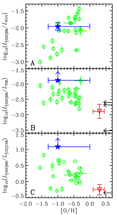
Figure 3: Comparisons of SXDF-NB1006-2 and other galaxies detected in the [O iii] line. The horizontal axis represents the oxygen abundance relative to the Sun on a logarithmic scale: $[{\rm O/H}]=\log_{10}(n_{\rm O}/n_{\rm H})-\log_{10}(n_{\rm O}/n_{\rm H})_{\odot}$, where $n_{\rm O}$ and $n_{\rm H}$ are the number density of oxygen and hydrogen atoms, respectively, and the solar abundance is assumed to be $12+\log_{10}(n_{\rm O}/n_{\rm H})_{\odot}=8.69$  (?). Circles with error bars represent data of nearby dwarf galaxies  (?, ?, ?); inverted triangles with error bars are averages of nearby spiral galaxies  (?). The arrows at the right-side axis show luminosity ratios of dusty galaxies at $z\sim 3$ to 4 whose oxygen abundances have not yet been measured  (?, ?, ?). Data from SXDF-NB1006-2 are shown as five-pointed stars with error bars. (A) The [O iii]/far ultraviolet (FUV) luminosity ratio. The FUV luminosity is $\nu L_{\nu}$ at about 1500 Å in the source rest-frame. (B) The [O iii]/total infrared (IR) luminosity ratio. The IR wavelength range is 8 to 1000 $\mu$m in the source rest-frame. Because the IR continuum of SXDF-NB1006-2 is not detected, we show a $3\sigma$ lower limit with a dust temperature of 40 K and an emissivity index of 1.5. (C) The [O iii]/[C ii] luminosity ratio. Because the [C ii] 158 $\mu$m line of SXDF-NB1006-2 is not detected, we show a $3\sigma$ lower limit.

The [O iii]/far-UV luminosity ratio of SXDF-NB1006-2 is similar to those of nearby dwarf galaxies with an oxygen abundance of 10% to 60% that of the Sun (Fig. 3A), which suggests that the oxygen abundance estimated from the SED modeling is reasonable and chemical enrichment in this young galaxy has already proceeded. On the other hand, the dust IR continuum and the [C ii] line of SXDF-NB1006-2 are very weak relative to those of the nearby dwarf galaxies (Fig. 3, B and C). The galaxies at $z\sim 3$ to 4, from which the [O iii] line was detected previously, are IR luminous dusty ones  (?, ?). Their [O iii]/IR and [O iii]/[C ii] luminosity ratios are similar to those of nearby spiral galaxies  (?) and are at least one order of magnitude smaller than those of SXDF-NB1006-2. The high [O iii]/IR ratio of SXDF-NB1006-2 despite a degree of chemical enrichment (or so-called metallicity) similar to that of the nearby dwarf galaxies indicates a very small mass fraction of dust in elements heavier than helium (or dust-to-metal mass ratio) in SXDF-NB1006-2. The dust deficiency of this galaxy is in contrast to the discovery of a dusty galaxy at $z\approx 7.5$  (?), suggesting a diversity of the dust content in the reionization epoch. Because the [C ii] line predominantly arises in gas where hydrogen is neutral, the non-detection of the [C ii] line in SXDF-NB1006-2 suggests that this young galaxy has little H i gas.

We also compared the observed properties of SXDF-NB1006-2 with the galaxies at $z=7.2$ in a cosmological hydrodynamic simulation of galaxy formation and evolution  (?). The simulation yielded several galaxies with a UV luminosity similar to that of SXDF-NB1006-2 (fig. S10). Relative to these simulated galaxies, SXDF-NB1006-2 has the highest [O iii] line luminosity, a similar oxygen abundance and a lower dust IR luminosity by at least a factor of 2 to 3. This indicates a factor of $>2$ to 3 smaller dust-to-metal mass ratio within the ISM of SXDF-NB1006-2 relative to that in the simulated galaxies where we assumed the dust-to-metal mass ratio of 50% as in the Milky Way ISM  (?). Therefore, the dust-to-metal ratio of SXDF-NB1006-2 is implied to be $<$20%. The dust-to-metal ratio is determined by two processes: dust growth by accretion of atoms and molecules onto the existing grains in cold dense clouds, and dust destruction by supernova (SN) shock waves consequent upon star formation  (?). The dust-poor nature of SXDF-NB1006-2 may be explained by rapid dust destruction due to its high SN rate or by slow accretion growth due to a lack of cold dense clouds in the ISM.

In the context of cosmic reionization studies, the most uncertain parameter is the product of the escape fraction of ionizing photons and the emission efficiency of these photons: $f_{\rm esc}\xi_{\rm ion}$  (?). From the SED modeling, we have obtained $\log_{10}(f_{\rm esc}\xi_{\rm ion}[{\rm Hz~{}erg^{-1}}])=25.44^{+0.46}_{-0.84}$ for SXDF-NB1006-2  (?). This ionizing photon emission efficiency is strong enough to reach (or even exceed) the cosmic ionizing photon emissivity at $z\sim 7$ estimated from various observational constraints on reionization  (?) by an accumulation of galaxies that have already been detected ($M_{\rm UV}<-17$), although this does not rule out contributions of fainter, currently undetected galaxies to the ionizing emissivity. The ISM properties of SXDF-NB1006-2, with little dust and H i gas, may make this galaxy a prototypical example of a source of cosmic reionization.

Acknowledgements

This paper makes use of the following ALMA data: ADS/JAO.ALMA# 2013.1.01010.S and 2012.1.00374.S which are available at https://almascience.nao.ac.jp/alma-data/archive. ALMA is a partnership of the European Southern Observatory (ESO) (representing its member states), NSF (USA) and NINS (Japan), together with NRC (Canada), NSC and ASIAA (Taiwan), and KASI (Republic of Korea), in cooperation with the Republic of Chile. The Joint ALMA Observatory is operated by ESO, the National Radio Astronomy Observatory/Associated Universities Inc., and the National Astronomical Observatory of Japan (NAOJ). Based in part on data collected at Subaru Telescope, which is operated by NAOJ; data are available at http://smoka.nao.ac.jp/ under project codes S08B-019, S08B-051, and S09B-055, and also at the W.M. Keck Observatory, which is operated as a scientific partnership among the California Institute of Technology, the University of California and NASA; data are available at www2.keck.hawaii.edu/koa/public/koa.php under the project code S331D. When some of the data reported here were acquired, UKIRT was operated by the Joint Astronomy Centre on behalf of the Science and Technology Facilities Council of the U.K.; UKIDSS data are available at http://wsa.roe.ac.uk//dr10plus_release.html. Based in part on archival data obtained with the Spitzer Space Telescope, which is operated by the Jet Propulsion Laboratory, California Institute of Technology under a contract with NASA; data are available at www.cfa.harvard.edu/SEDS/data.html.

Supported by JSPS KAKENHI grant numbers 26287034 (A.K.I. and K.M.), 26247022 (I.S.), 25287050 (N.Y.), 24740112 (T.O.), 15H02073 (Y.T.) and 15K17616 (B.H.), and by a grant-in-aid for JSPS Fellows (H.U.), by a grant-in-aid for the Global COE Program “The Next Generation of Physics, Spun from Universality and Emergence” from MEXT of Japan (K.O.), the Kavli Institute Fellowship at (Kavli Institute for Cosmology, University of Cambridge) supported by the Kavli Foundation (K.O.), and the Swedish Research Council (project 2011-5349) and the Wenner-Gren Foundations (E.Z.).

Supplementary Materials:

Materials and Methods

Figures S1-S12

Tables S1-S4

References (31-75)

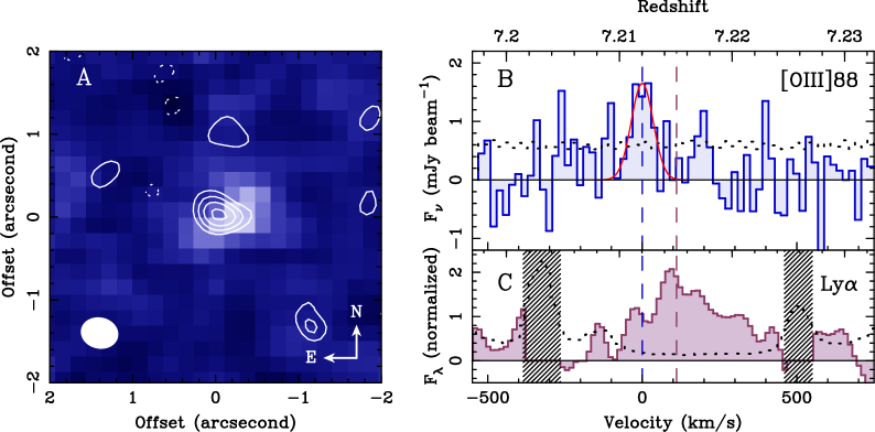
Figure 1: [O iii] 88 $\mu$m and Ly$\alpha$ emission images and spectra of SXDF-NB1006-2. (A) The ALMA [O iii] 88 $\mu$m image (contours) overlaid on the Subaru narrow-band Ly$\alpha$ image (offsets from the position listed in Table 1). Contours are drawn at ($-$2, 2, 3, 4, 5)$\times\sigma$, where $\sigma=0.0636$ Jy beam^-1 km s^-1. Negative contours are shown by the dotted line. The ellipse at lower left represents the synthesized beam size of ALMA. (B) The ALMA [O iii] 88 $\mu$m spectrum with resolution of 20 km s^-1 at the intensity peak position shown against the relative velocity with respect to the redshift $z=7.2120$ (blue dashed line). The best-fit Gaussian profile for the [O iii] line is overlaid. The RMS noise level is shown by the dotted line. (C) The Ly$\alpha$ spectrum  (?) shown as a function of the relative velocity compared to the [O iii] 88 $\mu$m line. The flux density is normalized by a unit of $10^{-18}$ erg s^-1 cm^-2 Å^-1. The sky level on an arbitrary scale is shown by the dotted line. The velocity intervals where Earth’s atmospheric lines severely contaminate the spectrum are flagged (hatched boxes). The Ly$\alpha$ line shows a velocity shift $\Delta v\approx+110$ km s^-1 relative to the [O iii] line (red dashed line).

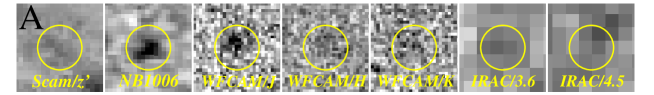
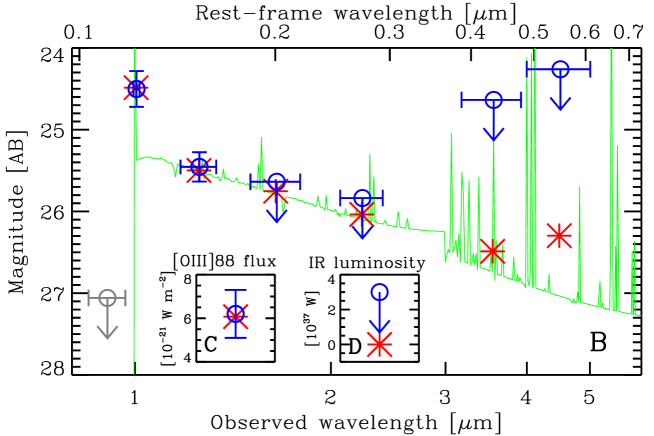
Figure 2: Spectral energy distribution of SXDF-NB1006-2. (A) Thumbnail images ($4^{\prime\prime}\times 4^{\prime\prime}$, north is up, east is to the left) in the Subaru/Suprime-Cam $z^{\prime}$, $NB1006$, UKIRT/WFCAM $J$, $H$, and $K$ bands, and Spitzer/IRAC 3.6-$\mu$m and 4.5-$\mu$m bands, from left to right. (B) Near-infrared photometric data with the best-fit model. The bottom horizontal axis shows the wavelength in the observer’s rest frame; the upper axis shows that in the source rest frame. The observations are marked by the circles. The horizontal error bars show the wavelength range of the band filters. The vertical error bars for detection bands represent $\pm 1\sigma$ photometric uncertainties; the downward arrows for non-detections represent the $3\sigma$ upper limits. The $z^{\prime}$ point in gray is not used for the model fit. The best-fit model spectrum is shown by the solid green line, and the corresponding magnitudes through the filters are indicated by asterisks. (C) The observed flux with the $\pm 1\sigma$ uncertainty of the [O iii] line and the best-fit model prediction (asterisk). (D) The $3\sigma$ upper limit on the total infrared luminosity with a dust temperature of 40 K and an emissivity index of 1.5. Also shown is the best-fit model prediction (asterisk; zero IR luminosity due to absence of dust in the best-fit model).

Table 1: A summary of the observed and estimated properties of SXDF-NB1006-2.

Right Ascension (J2000)	$2^{\mathrm{h}}18^{\mathrm{m}}56.536^{\mathrm{s}}$ ($\pm 0.002^{\mathrm{s}}$)
Declination (J2000)	$-5^{\circ}19^{\prime}58.87^{\prime\prime}$ ($\pm 0.02^{\prime\prime}$)
Redshift of [O iii] 88 $\mu$m	$7.2120\pm 0.0003$
Ly$\alpha$ velocity shift (km s-1)	$+1.1(\pm 0.3)\times 10^{2}$
$[$O iii$]$ 88 $\mu$m luminosity (W) ∗	$3.8(\pm 0.8)\times 10^{35}$
$[$C ii$]$ 158 $\mu$m luminosity (W) ∗	$<3.2\times 10^{34}$ ($3\sigma$)
Total IR luminosity (W) ∗	$<2.9\times 10^{37}$ ($3\sigma$)
Oxygen abundance $[\rm O/H]$	$-1.0^{+1.0}_{-0.3}$
Star formation rate (log10 M⊙ yr-1) †	$2.54_{-0.71}^{+0.17}$
Star formation age (log10 yr)	$6.00^{+1.00}$
Dust attenuation ($E_{B-V}$ mag)	$0.00^{+0.04}$
Escape fraction of ionizing photons	$0.54_{-0.54}^{+0.17}$
Stellar mass (log10 M⊙) †	$8.54_{-0.22}^{+0.79}$

^∗ Assuming a concordance cosmology with $H_{0}=70$ km s^-1 Mpc^-1, $\Omega_{\rm M}=0.3$, and $\Omega_{\Lambda}=0.7$.

^† M_⊙ represents the Solar mass ($1.989\times 10^{30}$ kg.)

Supplementary Materials for

Detection of an oxygen emission line from a high redshift galaxy in the reionization epoch

Akio K. Inoue, Yoichi Tamura, Hiroshi Matsuo, Ken Mawatari, Ikkoh Shimizu, Takatoshi Shibuya, Kazuaki Ota, Naoki Yoshida, Erik Zackrisson, Nobunari Kashikawa, Kotaro Kohno, Hideki Umehata, Bunyo Hatsukade, Masanori Iye, Yuichi Matsuda, Takashi Okamoto, Yuki Yamaguchi

Correspondence to: akinoue@las.osaka-sandai.ac.jp

The PDF file includes:

Materials and Methods

Figs. S1 to S12

Tables S1 to S4

Materials and Methods

1 ALMA observation and results

1.1 Observations and data reduction

The ALMA band 8 data of the [O iii] 88 $\mu$m emission line (rest-frame frequency 3393.01 GHz) redshifted to 413 GHz for the target galaxy, SXDF-NB1006-2, were obtained on 2015 June 7, 9 and 14 (cycle 2, project ID: 2013.1.01010.S, PI: A. K. Inoue). Thirty-seven to 41 operational antennas were employed with the C34-6/7 array configuration, where the maximum and minimum baseline lengths were 783.5 m and 21.3 m, respectively. The correlator was configured so that 400.1–403.6 and 412.1–414.0 GHz were covered by four spectral windows, each of which was used in the Frequency Division Mode (FDM) with a 1.875 GHz bandwidth and a 7.8125 MHz (5.67 km s^-1 at 413 GHz) resolution. A total of 2.0 hour was spent for on-source integration under excellent atmospheric conditions with precipitable water vapors (PWVs) of 0.4–0.5 mm. The resulting spatial resolution with the natural weighting is $0.^{\prime\prime}35\times 0.^{\prime\prime}26$ (in full width at half maximum (FWHM); position angle PA = $+82^{\circ}$), with the r.m.s. noise levels of 0.53 and 0.042 mJy beam^-1, respectively, for the 20 km s^-1 resolution cube and the continuum image. Two quasars, J0241$-$0815 ($S_{\mathrm{413\,GHz}}=1.6$ Jy, 6^∘ away from the target) and J2232+1143 (0.3 Jy), and Ceres were used for complex gain, bandpass and flux calibration, respectively. The flux calibration accuracy is estimated at 10%.

The band 6 data targeting the [C ii] 158 $\mu$m line (the rest-frame frequency of 1900.54 GHz) at 231 GHz for SXDF-NB1006-2 were obtained on 2014 August 1 and 5 (cycle 1, project ID: 2012.1.00374.S, PI: K. Ota), where 30–34 antennas were operational under the C32-5 configuration (the maximum and minimum baseline lengths of 558.2 m and 17.2 m, respectively). The correlator was configured to cover 215.7–219.5 and 230.4–234.2 GHz in the FDM 1.875 GHz mode with a 0.488 MHz (0.63 km s^-1 at 231 GHz) resolution. The conditions were reasonable (PWV = 1–2 mm) during the on-source time of 1.8 hour. The resulting synthesized beam size (FWHM) with the natural weighting is $0.^{\prime\prime}80\times 0.^{\prime\prime}60$ (PA = $-81^{\circ}$). The achieved noise levels for the 20 km s^-1 cube and the continuum image are 0.26 and 0.014 mJy beam^-1, respectively. Complex gain calibration was made using a nearby quasar J0215$-$0222 ($S_{\mathrm{231~{}GHz}}=0.06$ Jy, $4^{\circ}$ away from the target), while three quasars (J0006$-$0623, J0423$-$0120 and J0241$-$0815) were used for bandpass calibration. Both Neptune and J0238+166 were used for flux calibration to cross-check the amplitude scaling. The flux calibration accuracy is estimated at 8%.

We calibrated the raw visibility data in a standard manner using the CASA software  (?) version 4.3.1 and 4.2.1 for the [O iii] and [C ii] data, respectively, along with a standard calibration script provided by the observatory. In addition to standard flagging such as shadowed antennas, manual flagging has carefully been made for low-gain antennas and abnormal visibilities. For the [O iii] (band 8) data, Earth’s atmospheric ozone lines severely affect up to 10% of the frequency coverage in 3 out of 4 spectral windows and are flagged properly, while the rest of the spectral window where the [O iii] line is expected does not suffer from the atmospheric contamination and remains unflagged.

Imaging is carried out using a CASA task, clean, with the natural weighting to maximize the point-source sensitivities. Continua are not subtracted in [O iii] and [C ii] imaging because no continuum emission is found. As the [O iii] emission is found to be marginally resolved with the naturally-weighted beam (the intrinsic source size from a Gaussian fit of $0.^{\prime\prime}4\times 0.^{\prime\prime}3$, PA $\simeq 90^{\circ}$), we also make a $uv$-tapered image with outertaper = $0.^{\prime\prime}3$ to achieve a good detection. The resulting beam size is $0.^{\prime\prime}45\times 0.^{\prime\prime}38$ (PA = $+78^{\circ}$). Synthesized-beam deconvolution was made for the [O iii] image using the CLEAN algorithm down to a $1.5\sigma$ level.

1.2 Results

1.2.1 [O iii] 88 $\mu$m line

The [O iii] emission is detected at a significance of $5.3\sigma$ at the position where the Ly$\alpha$ emission is detected (Figure 1A). The $uv$-tapered image is integrated over $-300$ to $+230$ km s^-1 with respect to the [O iii] redshift of $z_{\mathrm{[OIII]}}=7.2120$, which is obtained by a Gaussian fit to the spectrum of a velocity resolution of 20 km s^-1. The histogram of pixel signal-to-noise ratios (SNRs) in the [O iii] integrated intensity image (Figure S1) is well described by a Gaussian (i.e., normal distribution) at the pixel values below SNR $<4$, while the number of pixels with positive fluxes surpasses that of the negative pixels at SNR $>4$. This is due to the contribution from the real [O iii] emission line. To further test the significance of the detection, we separately image the data taken during three independent tracks made on 2015 June 7, 9 and 14. The on-source time of each track is 40 min. We find a $\sim 3\sigma$ peak at the position of SXDF-NB1006-2 in every image, demonstrating a robust detection of the [O iii] line (Figure S2).

Figure S1: Histogram of pixel signal-to-noise ratios (SNRs) of the [O iii] integrated intensity map. The data are taken from the entire field of view of ALMA band 8 observations. Positive flux values are shown by the red solid line, while negative values are shown by the blue dashed line. The histograms are well described by a Gaussian up to SNRs around 4, whereas there is an excess in positive flux values at SNR $>4$, to which the [O iii] emission contributes.

Figure S2: [O iii] 88 $\mu$m integrated intensity maps of each observing date. Every image shows a $\sim 3\sigma$ peak at the position where the [O iii] line is found (crosses), demonstrating the detection robustness. Contours start from $1\sigma$ with a step of $1\sigma$. The dotted contours show negative values. The ellipse at the bottom-left corner on each panel indicates the ALMA beam size.

Figure S3: [O iii] 88 $\mu$m spectra at the intensity peak with different velocity resolutions. From A to C, the velocity resolution is 35, 20 and 10 km s^-1. The dotted line is the r.m.s. noise level measured over each resolution element. In panel A, the Ly$\alpha$ redshift is indicated with the upward arrow. The vertical bands in red, green and blue represent the velocity intervals over which the integrated intensity images shown in Figure S5 are integrated. In the panel B, we show the best-fit Gaussian profile for the emission line. The FWHM is $\approx 80$ km s^-1.

In the band 8 spectra at the intensity peak position, a narrow (FWHM of $\approx 80$ km s^-1) line feature is evident at around 413.2 GHz (Figure S3B). This line feature is neither a collection of spurious spikes nor a part of spectral baseline wiggles (Figure S3C). The redshift of the line is measured as $z_{\rm[OIII]}=7.2120\pm 0.0003$, slightly lower than the redshift determined from the Ly$\alpha$ emission line  (?). This redshift difference corresponds to a velocity offset of $\approx 110$ km s^-1 (§2.1), which is reasonably accounted for when the bluer (i.e., shorter-wavelength) part of the Ly$\alpha$ emission line is attenuated by the IGM along the sightline, as reported for many Ly$\alpha$ emitters at $z\sim 6$–7  (?, ?), in addition to the ISM attenuation  (?, ?, ?).

We measure the total flux density of the [O iii] emission by fitting the tapered integrated intensity image to a Gaussian using a CASA task, imfit, and deconvolving the clean beam to derive the intrinsic source flux. Table S1 lists the integrated intensity ($0.45\pm 0.09$ Jy km s^-1, which corresponds to a flux of $6.2\times 10^{-21}$ W m^-2) and luminosity ($9.8\times 10^{8}~{}L_{\odot}$), where $L_{\odot}=3.8\times 10^{26}$ W is the solar luminosity. The [O iii] line luminosity is at the high end of the detections made in local dwarf galaxies  (?), normal spirals  (?) and (ultra-)luminous infrared galaxies  (?), while it is an order of magnitude lower than (demagnified) [O iii] line luminosities found in gravitationally-lensed dusty starburst galaxies at $3<z<4$  (?, ?).

Table S1: ALMA results of [O iii] 88 $\mu$m and [C ii] 158 $\mu$m lines of SXDF-NB1006-2.
[O iii] 88 $\mu$m [C ii] 158 $\mu$m Integrated intensity (Jy km s^-1) $0.45\pm 0.09$ $<0.069$ $(3\sigma)$ Flux calibration uncertainty $10\%$ $8\%$ Flux (W m^-2) $(6.2\pm 1.4)\times 10^{-21}$ ^† $<5.3\times 10^{-22}$ $(3\sigma)$ Luminosity ($L_{\odot}$) ^∗ $(9.8\pm 2.2)\times 10^{8}$ ^† $<8.3\times 10^{7}$ $(3\sigma)$ Beam-deconvolved source size $0.4^{\prime\prime}\times 0.3^{\prime\prime}$ (PA $\simeq 90^{\circ}$) —

^∗ Assuming a concordance cosmology with $H_{0}=70$ km s^-1 Mpc^-1, $\Omega_{\rm M}=0.3$, and $\Omega_{\Lambda}=0.7$.

^† Flux calibration uncertainty is included in the error.

1.2.2 [C ii] 158 $\mu$m line

In the integrated intensity map of the [C ii] emission summed over the same velocity range as that of the [O iii] image, we find no [C ii] emission with a $>3\sigma$ significance around SXDF-NB1006-2 (Figure S4A). Thus, we conclude that there is no significant [C ii] line source integrated over the same velocity range as the [O iii] line at the position emitting the [O iii] and hydrogen Ly$\alpha$ lines. Thus, we place a $3\sigma$ upper limit on flux and luminosity for the [C ii] line (Table S1). On the other hand, we notice that when the band 6 cube is integrated over two velocity ranges, $-20<v<260$ and $90<v<230$ km s^-1, low-significance ($3.5\sigma$ and $3.7\sigma$) bumps appear close to the LAE (denoted as ‘NE’ and ‘SE’ in Figure S4B and S4C, respectively). Unfortunately, the features are severely affected by the Earth’s atmospheric ozone line at 231.28 GHz, which prevents us from judging whether or not these are spurious. Furthermore, there are a few more $3\sigma$–$4\sigma$ enhancements remaining over the map (see a $3.9\sigma$ enhancement at the northern edge of Figure S4A).

Figure S4: [C ii] 158 $\mu$m emission line integrated intensity maps of SXDF-NB1006-2. (A) The integrated intensity image of the [C ii] line over the same velocity range as that of the [O iii] line ($-300<v<+230$ km s^-1). The black contours represent ($\pm 1$, $\pm 2$, $\pm 3$, …)$\times\sigma$, where $\sigma=$ 28 mJy beam^-1 km s^-1. Negative contours are shown by dotted lines. The white contours show the [O iii] line image and are drawn at $2\sigma$ and $4\sigma$. No significant [C ii] emission is found. (B) The same as A but integrated over $-20<v<+260$ km s^-1 ($\sigma=$ 23 mJy beam^-1 km s^-1). The inset shows the spectrum at the marginal $3.5\sigma$ enhancement north-east to the [O iii] position (denoted as ‘NE’). The dotted line with gray shade shows the $1\sigma$ noise level. The frequency range where an atmospheric absorption line contaminates the spectrum is indicated by a hatched band. (C) The same as A but integrated over $+90<v<+260$ km s^-1 ($\sigma=$ 21 mJy beam^-1 km s^-1). The inset shows the spectrum at the marginal $3.7\sigma$ enhancement south-east to the [O iii] position (denoted as ‘SE’).

1.2.3 Dust continuum

Continuum emission remains undetected in both the band 8 (735 $\mu$m) and band 6 (1.33 mm) images. The $3\sigma$ upper limits measured for naturally-weighted images are 0.12 and 0.042 mJy at 735 $\mu$m and 1.33 mm, respectively. The total IR luminosity assuming a modified blackbody  (?) integrated over the rest-frame wavelengths of 8–1000 $\mu$m is estimated to be $L_{\rm TIR}<1\times 10^{11}~{}L_{\odot}$, where the dust temperature and emissivity index are assumed to be $T_{\rm dust}=40$ K and $\beta=1.5$, respectively. This limit can be relaxed to $<2\times 10^{11}~{}L_{\odot}$ for a higher dust temperature of $T_{\mathrm{dust}}=50$ K, while if the galaxy has cooler dust ($T_{\mathrm{dust}}=30$ K), the luminosity limit obtained from the 1.33 mm photometry becomes more stringent ($<4\times 10^{10}~{}L_{\odot}$). Table S2 is a summary of these results. The emissivity index of 1.5 which we assumed is a typical value observed in nearby star-forming galaxies  (?). It is reported that the typical star-forming galaxies ($L\sim L_{*}$) at $z\sim 4$ have $T_{\rm dust}\simeq 30$ K  (?). A bright LAE at $z\simeq 7$, Himiko  (?), is estimated to have $T_{\rm dust}=30$–40 K  (?). We therefore assume $T_{\rm dust}=40$ K as a fiducial value for SXDF-NB1006-2 in this paper. For this temperature, the effect of the cosmic microwave background whose temperature is 22 K at $z=7.2$ is small  (?).

Table S2: ALMA results of the dust IR continuum of SXDF-NB1006-2.
Band 8 (735 $\mu$m) Band 6 (1.33 mm) Flux density (mJy) $<0.12$ ($3\sigma$) $<0.042$ ($3\sigma$) Dust temperature (K) Total infrared luminosity ($L_{\odot}$, $3\sigma$) ^∗ 30 $<9.0\times 10^{10}$ $<3.8\times 10^{10}$ 40 $<1.1\times 10^{11}$ $<8.3\times 10^{10}$ 50 $<1.7\times 10^{11}$ $<1.7\times 10^{11}$

^∗ We assume a single-temperature modified blackbody with an emissivity index of 1.5 and a concordance cosmology with $H_{0}=70$ km s^-1 Mpc^-1, $\Omega_{\rm M}=0.3$, and $\Omega_{\Lambda}=0.7$.

1.2.4 Possible kinematics signature in the [O iii] spectrum

The [O iii] image (Figure 1A) is marginally resolved and likely elongated in the east–west direction. The beam-deconvolved source size, if the source is approximated by a two-dimensional Gaussian, is estimated to be $0.^{\prime\prime}4\times 0.^{\prime\prime}3$ in FWHM (PA $\sim 90^{\circ}$), corresponding to a physical scale of $\simeq 2\times 1.5$ kpc². This extended structure may be attributed to high-velocity components that are seen as red-shifted and blue-shifted marginal broad signals in the [O iii] spectrum (Figure S3A). We made images of the central narrow component ($-50<v<+50$ km s^-1) and the red-shifted and blue-shifted marginal high-velocity components ($50<v<230$ km s^-1 and $-300<v<-50$ km s^-1; Figure S5). Although the SNR is not high enough, it seems that the high-velocity components are mostly overlapped but exhibit a small spatial offset of $0.^{\prime\prime}3$ ($\simeq 1.5$ kpc), which is larger than the statistically-expected positional uncertainty ($\simeq 0.5\theta/\mathrm{SNR}\simeq 0.05^{\prime\prime}$, where $\theta$ is the beam size).

Figure S5: Spatial distribution of different velocity components of the [O iii] 88 $\mu$m emission. Red and blue contours show the red-shifted ($50<v<230$ km s^-1) and blue-shifted ($-300<v<-50$ km s^-1) marginal components, respectively, while white contours represent the narrow component ($-50<v<+50$ km s^-1) which likely traces the systemic redshift of SXDF-NB1006-2. These velocities are measured with respect to the [O iii] line peak at $z=7.2120$. Contours are drawn at ($\pm 1$, $\pm 2$, $\pm 3$, …)$\times\sigma$ for the high-velocity components and ($\pm 2$, $\pm 3$)$\times\sigma$ for the narrow component for clarity. Negative contours are shown by the dotted lines. The background image is the Subaru narrowband Ly$\alpha$ image  (?). The ellipse at the bottom-left corner represents the naturally-weighted beam size of ALMA.

A possible explanation of these marginal high-velocity component is rotating motion of gravitationally-bounded gas, which is often observed in high-$z$ massive galaxies  (?, ?). A dynamical mass is an order of $M_{\rm dyn}\sim 1\times 10^{5}~{}v_{\rm circ}^{2}D$ M_⊙, where $v_{\rm circ}=0.75~{}\Delta v~{}(\sin{i})^{-1}$ is the circular velocity in units of km s^-1 ($\Delta v$ and $i$ are, respectively, the line FWHM and the inclination angle) and $D$ is the diameter of the galaxy measured in kpc. If the possible red/blue-shifted components of the [O iii] line is produced by a rotating disk with a $D\simeq 2$ kpc and a velocity width of $\Delta v=400$ km s^-1 (FWHM), the dynamical mass is estimated to be $M_{\rm dyn}\sim 5\times 10^{10}~{}M_{\odot}$, where we assume that the galaxy is a circular disk and the intrinsic source size gives the inclination angle, i.e., $i=\cos^{-1}{(0.^{\prime\prime}3/0.^{\prime\prime}4)}$. The dynamical mass is 2 orders of magnitude larger than the best-fit stellar mass obtained from the SED fitting (§3.5). However, it can not be excluded that a passive stellar population of $<5\times 10^{10}$ M_⊙ coexists with a young starburst in SXDF-NB1006-2 (Figure S11). In a cosmological simulation  (?, ?), galaxies at $z=7.2$ with similar UV luminosities to SXDF-NB1006-2 have a stellar mass of a few $\times 10^{10}$ M_⊙ (see §4, Figure S10) and a dark halo mass of a few $\times 10^{11}$ M_⊙. Therefore, the high-velocity component could be explained by rotational motion.

Another interpretation is violent motions such as outflows driven by stellar winds and supernovae in the star forming region of SXDF-NB1006-2, which is probably seen as the narrow component (FWHM of $\approx 80$ km s^-1). Yet another possibility is turbulent motion driven by, for example, a merger event which might mimic the spatial offset, although we find a single unresolved component in the $J$ band image tracing the rest-frame UV continuum (Figure 2A). However, we can not conclude the origin of the possible high-velocity components because of the limited SNR for the moment.

2 Optical-to-near infrared data

The target galaxy, SXDF-NB1006-2, is in the Subaru/XMM-Newton Deep Survey Field (SXDF)  (?) where multi-wavelength deep observations have been carried out. We have gathered archival optical-to-near infrared (NIR) deep images available in the SXDF: Subaru/Suprime-Cam broadband $z^{\prime}$  (?) and narrowband $NB1006$  (?), UKIRT/WFCAM broadband $J$, $H$, and $K$ taken in the UKIRT Infrared Deep Sky Survey (UKIDSS) Ultra-Deep Survey (UDS)  (?), and Spitzer/IRAC $3.6~{}\mu$m and $4.5~{}\mu$m taken in the Spitzer Extended Deep Survey (SEDS)  (?). We measured the point spread functions (PSFs) using stellar objects in these images, resulting in FWHMs of $1.^{\prime\prime}0$ ($z^{\prime}$), $0.^{\prime\prime}4$ ($NB1006$), $0.^{\prime\prime}8$ ($J$, $H$, and $K$), and $1.^{\prime\prime}8$ ($3.6\mu$m and $4.5\mu$m). Except for the $NB1006$ image, the photometry was performed using $2\times$PSF (FWHM) apertures because the object is almost unresolved or not detected. For the $NB1006$ image, we performed Kron photometry  (?) with the parameter $k=2$ to obtain a total flux density from the spatially extended Ly$\alpha$ emission. The photometric measurements are summarized in Table S3. The magnitudes are the AB system  (?).

Table S3: Photometric data of SXDF-NB1006-2. Band Wavelength ($\mu$m) PSF FWHM (^′′) Magnitude (AB) $z^{\prime}$ 0.91 $1.^{\prime\prime}0$ $>27.06$ ^∗ $NB1006$ 1.00 $0.^{\prime\prime}4$ $24.50\pm 0.22$ ^† $J$ 1.26 $0.^{\prime\prime}8$ $25.46\pm 0.18$ ^‡ $H$ 1.65 $0.^{\prime\prime}8$ $>25.64$ ^∗ $K$ 2.23 $0.^{\prime\prime}8$ $>25.84$ ^∗ $IRAC3.6$ 3.54 $1.^{\prime\prime}8$ $>24.64$ ^∗ $IRAC4.5$ 4.49 $1.^{\prime\prime}8$ $>24.26$ ^∗

^∗ 3$\sigma$ lower limit in $2\times$PSF circular aperture.

^† Kron magnitude with a $2.^{\prime\prime}64\times 1.^{\prime\prime}32$ ellipse aperture.

^‡ $2\times$PSF circular aperture.

2.1 Velocity offset between Ly$\alpha$ and [O iii] lines

We have performed a profile fitting of the Ly$\alpha$ line with an asymmetric Gaussian function  (?):

$$F_{\lambda}=A\exp\left[\frac{-(\lambda-\lambda_{0})^{2}}{2\{\sigma+a(\lambda-\lambda_{0})\}^{2}}\right]\,,$$ (1)

where $A$ is the peak flux, $\lambda_{0}$ is the peak wavelength, $\sigma$ is the line width, and $a$ is the asymmetric parameter. If $a>0$, the blue part of the line profile is weakened as the Ly$\alpha$ line observed in high-$z$  (?). The usual Gaussian function is recovered with $a=0$. First, we have made a fitting with a Gaussian function and obtained the following results: $A=(1.67\pm 0.15)\times 10^{-18}$ erg s^-1 cm^-2 Å^-1, $\lambda_{0}=9987.51\pm 0.822$ Å, and $\sigma=4.71\pm 0.42$ Å (Figure S6). The corresponding redshift is $z_{\rm Ly\alpha}=7.2156\pm 0.0007$ (Gaussian fit). Next, we have made a fitting with an asymmetric Gaussian function with a fixed $\sigma=4.71$ Å from the Gaussian fit, which is also consistent with the observed FWHM of the line (11.5 Å  (?)). The results are $A=(1.65\pm 0.16)\times 10^{-18}$ erg s^-1 cm^-2 Å^-1, $\lambda_{0}=9986.67\pm 0.967$ Å, and $a=0.169\pm 0.065$ (Figure S6). The corresponding redshift is $z_{\rm Ly\alpha}=7.2150\pm 0.0008$ (asymmetric Gaussian fit). Assuming that the [O iii] 88 $\mu$m line at $z_{\rm[OIII]}=7.2120\pm 0.0003$ traces the systemic redshift, we have obtained the velocity offset of the Ly$\alpha$ line $\Delta v_{\rm Ly\alpha}=+(1.1\pm 0.3)\times 10^{2}$ km s^-1, where we have corrected the Ly$\alpha$ redshift for the heliocentric motion of Earth at the observing date ($+4$ km s^-1). Note that the ALMA spectrum of the [O iii] line is already corrected for the Earth’s motion in the data reduction process.

Figure S6: Ly$\alpha$ line profile fitting results. The black solid line is the observed spectrum and the red solid line is the best-fit profile with an asymmetric Gaussian function expressed in equation (1). The cyan dashed line is the best-fit result with a simple Gaussian function for a reference. The central wavelengths with their $\pm 1\sigma$ uncertainties are shown by the upward arrows with error-bars. The wavelength range used in the fitting is 9975–9998 Å. The top horizontal axis is the velocity shift relative to the systemic redshift $z=7.2120$ measured from the [O iii] 88 $\mu$m line and corrected for the heliocentric motion of Earth.

2.2 Empirical SFR estimation

We now estimate the SFR of SXDF-NB1006-2 with empirical relations. We assume a Salpeter initial mass function (IMF)  (?) with the mass range of 0.1–100 M_⊙ throughout this paper. There is a good correlation between the [O iii] 88 $\mu$m line luminosity and the SFR derived from the sum of the FUV and IR luminosities based on a large compilation of various kinds of galaxies including nearby low-metallicity dwarfs, ULIRGs, AGNs, and high-$z$ dusty starbursts  (?). The [O iii]–SFR relations for specific kinds of galaxies are slightly different from each other. If we assume the relation derived from the entire sample of  (?), we obtain a SFR $>100$ M_⊙ yr^-1 for SXDF-NB1006-2 (Figure S7). On the other hand, the $J$ band (i.e. rest-frame $\approx 1500$ Å) luminosity of this galaxy indicates a SFR $\sim 10$ M_⊙ yr^-1 with a standard FUV–SFR conversion  (?). This conversion assumes a constant SFR more than a few 100 Myr, while it actually depends on the duration of star formation. If the star formation age is $\sim 1$ Myr, we indeed obtain $\sim 100$ M_⊙ yr^-1 which is consistent with the estimation based on the [O iii] line. This suggests that the target galaxy is in a young violent star formation phase.

Figure S7: Empirical relation between the SFR and the [O iii] 88 $\mu$m line luminosity  (?). The best-fit relation with $\pm 1\sigma$ standard deviation for a large compilation of the data of various kinds of galaxies including low-metallicity nearby dwarf galaxies (circles) and $z\sim 3$–4 dusty starburst galaxies (diamonds) is shown by the yellow line with the gray shade. The [O iii] line luminosity with $\pm 1\sigma$ uncertainty of SXDF-NB1006-2 at $z=7.2$ is shown by the horizontal blue line with the orange shade. The crosses show SFRs estimated from the observed FUV luminosity of the target galaxy, under various assumptions on the duration of star formation. All the SFRs are calibrated to ones with the Salpeter IMF  (?) with 0.1–100 M_⊙.

3 Spectral energy distribution modeling

In order to derive physical properties of the galaxy, SXDF-NB1006-2, we have performed a spectral energy distribution (SED) fitting  (?, ?). This is based on a standard $\chi^{2}$ minimization method:

$$\chi^{2}=\sum_{i=1}^{N}\left(\frac{F_{i,{\rm model}}-F_{i,{\rm obs}}}{\sigma_{i,{\rm obs}}}\right)^{2}\,,$$ (2)

where $F_{i,{\rm model}}$, $F_{i,{\rm obs}}$, and $\sigma_{i,{\rm obs}}$ are the model flux density (or flux), the observed flux density (or flux) and the observed uncertainty of $i$th data point, respectively. We have used not only the broadband photometric data ($J$, $H$, $K$, $IRAC3.6$ and $IRAC4.5$) but also the narrowband $NB1006$ photometry, the [O iii] 88 $\mu$m line flux and the total IR flux upper limit as constraints. For non-detection bands and the IR flux, we simply set $F_{i,{\rm obs}}=0$ and take their $3\sigma$ limits as $\sigma_{i,{\rm obs}}$. This treatment makes the fitting favor $F_{i,{\rm model}}$ below the $3\sigma$ limits for the non-detection data. There are other choices to manage the non-detection data, for example, taking $F_{i,{\rm obs}}=\sigma_{i,{\rm obs}}=1.5\sigma$ limit (option 2 of  (?)) or a modification of equation (2) to treat the upper limits  (?). We have tried these two methods and found that the best-fit parameters do not change but their $1\sigma$ ranges tend to be smaller. This is because the latter two methods put a larger weight on the non-detection data. Thus, our approach above is more conservative than the latter two methods. The $z^{\prime}$ band which is severely affected by the intergalactic attenuation is omitted because we have fixed the redshift to that of the [O iii] line ($z=7.212$) and the non-detection in the $z^{\prime}$ band does not have much information. Therefore, the number of the constraints is $N=8$.

3.1 Stellar continuum

We have adopted theoretical spectra generated with a public stellar population synthesis code PEGASE ver. 2  (?). We assume metallicities of $Z=0.0004$, 0.001, 0.002, 0.004, 0.008, 0.02, and 0.05 with a classical solar metallicity of $Z=0.02$  (?). The stellar IMF is assumed to be a standard Salpeter one  (?) with the range of 0.1–100 M_⊙. A constant star formation history is also assumed for simplicity. In this case, the obtained age and stellar mass are regarded as those of the most recent star formation episode. If the galaxy has previous star formation episodes, the true age and stellar mass are larger than those obtained here. On the other hand, for instantaneous quantities such as the SFR and dust attenuation, the assumption of a constant SFR is valid in the sense of an average during the star formation episode. We have set a lower limit of 1 Myr in the age. Metallicity evolution, gas infall, outflow, nebular emission, and dust extinction have not been considered at this stage.

3.2 Nebular emission

The spectra of young star-forming galaxies are significantly affected by emission from ionized gas, so-called nebular emission  (?). We have added the nebular continuum (two-photon, bound-free, and free-free continua) and 119 UV-to-optical ($\lambda<1$ $\mu$m in the source rest-frame) emission lines to the model spectra following the prescription of  (?, ?). This emission line model is based on a large set of calculations of H ii regions using a public photoionization code, cloudy  (?) and reproduces the observed strengths of several prominent emission lines such as [O iii] $\lambda$5007 relative to the hydrogen H$\beta$ line very well. For the [O iii] 88 $\mu$m line, the model presented in  (?) is adopted. This [O iii] line model is also made with cloudy and agrees with the available observations of the [O iii] 88 $\mu$m line very well (Figure S8).

Figure S8: Emissivity of the [O iii] 88 $\mu$m line per a unit SFR as a function of the oxygen abundance. The horizontal axis is the oxygen abundance relative to that of the Sun ($[{\rm O/H}]=\log_{10}(n_{\rm O}/n_{\rm H})-\log_{10}(n_{\rm O}/n_{\rm H})_{\odot}$ with $12+\log_{10}(n_{\rm O}/n_{\rm H})_{\odot}=8.69$)  (?). The data of nearby dwarf galaxies come from observations with the Herschel satellite  (?, ?, ?). The data of LMC and nearby spiral galaxies as well as model predictions are taken from  (?). We show the models with the ionization parameter $\log_{10}U$ and the hydrogen atom density $\log_{10}n_{\rm H}$ noted in the panel. The SFR is calibrated to ones with the Salpeter IMF with 0.1–100 M_⊙.

We allow the escape of hydrogen ionizing photons (wavelength $\lambda<912$ Å in the source rest-frame; Lyman continuum) from H ii regions and the surrounding ISM in the galaxy to the IGM. Not only the stellar ionizing photons but also nebular bound-free ionizing photons can escape to the IGM  (?). We assume that both escapes happen with the same escape fraction, $f_{\rm esc}$, defined as the number fraction of the escaped photons among the produced photons.

3.3 Dust attenuation and IR luminosity

We assume the Calzetti attenuation law  (?, ?) for the attenuation by dust particles in the ISM as a standard manner found in literature, while recent studies may suggest deviations from the Calzetti law in high-$z$ galaxies  (?, ?). Fortunately, the obtained attenuation amount for the target galaxy is small and the shape of the attenuation law would not affect the conclusions of this paper.

The Calzetti law predicts about a factor of 2 higher attenuation for the nebular emission than for the stellar continuum. This is because H ii regions producing the nebular emission are more deeply embeded in gas and dust clouds than stars observed in the UV wavelength. On the other hand, such a difference between nebular and stellar emissions may not be supported by observations of young star-forming galaxies  (?, ?). We then introduce a parameter, $R_{\rm gs}\equiv(E_{B-V})_{\rm gas}/(E_{B-V})_{\rm star}$, to describe this effect and assume $R_{\rm gs}=1$ or 2. The original Calzetti law predicts $R_{\rm gs}=2.3$.

We assume that the radiation energy attenuated by dust is finally absorbed by dust in the ISM and thermally re-emitted in the IR (i.e., we assume the energy scattered out to the IGM to be negligible). This energy is compared to the total IR luminosity estimated with the dust temperature of 40 K (Table 1), assuming the total dust emission comes only from the star-forming regions of interest.

3.4 Ly$\alpha$ emission line

The narrowband $NB1006$ photometry is mainly determined by the Ly$\alpha$ emission line although it also contains information of the UV continuum. Since Ly$\alpha$ photons suffer from resonant scattering by neutral hydrogen, the transfer in the ISM is complex. In addition to the ISM, Ly$\alpha$ photons are also scattered by neutral hydrogen in the IGM. Therefore, the observed Ly$\alpha$ flux becomes $F_{\rm Ly\alpha}^{\rm obs}=F_{\rm Ly\alpha}^{\rm int}T_{\rm Ly\alpha}^{\rm IGM}e^{-\tau^{\rm ISM}_{\rm Ly\alpha}}$, where $F_{\rm Ly\alpha}^{\rm int}$ is the intrinsic Ly$\alpha$ flux, $\tau_{\rm Ly\alpha}^{\rm ISM}$ and $T_{\rm Ly\alpha}^{\rm IGM}$ are, respectively, the ISM optical depth and the IGM transmission for Ly$\alpha$ photons. Recent studies of LAEs suggest that a simple recipe like the Calzetti law with $R_{\rm gs}\simeq 1$ (i.e. $(E_{B-V})_{\rm gas}=(E_{B-V})_{\rm stars}$) reasonably explains the Ly$\alpha$ optical depth in the ISM inferred from the Ly$\alpha$ line profile  (?). The IGM effect is more severe at higher redshift due to a higher neutral fraction in the IGM. At redshift $z\simeq 7.2$, the neutral fraction, $x_{\rm HI}$, in the IGM is estimated to be $\sim 0.5$  (?) although it is still uncertain. According to a cosmological radiative transfer simulation, the Ly$\alpha$ transmission through the IGM with an average $x_{\rm HI}=0.5$ is $T_{\rm Ly\alpha}^{\rm IGM}=0.35_{-0.15}^{+0.10}$  (?). Since this $T_{\rm Ly\alpha}^{\rm IGM}$ range also covers a wide range of $x_{\rm HI}=0.2$–0.8  (?), we assume that the $T_{\rm Ly\alpha}^{\rm IGM}$ range encloses the uncertainty of $x_{\rm HI}$.

3.5 Results

We use $N=8$ observational constraints: 6 photometric data ($NB1006$, $J$, $H$, $K$, $IRAC3.6$ and $IRAC4.5$) and the [O iii] 88 $\mu$m line flux and the total IR flux. On the other hand, there are 7 model parameters: the metallicity $Z$, the IGM Ly$\alpha$ transmission $T_{\rm Ly\alpha}^{\rm IGM}$, the dust attenuation ratio of nebular to stellar emissions $R_{\rm gs}$, the SFR, the age, the stellar dust attenuation $(E_{B-V})_{\rm star}$, and the escape fraction of ionizing photons $f_{\rm esc}$. For the first 3 parameters, we fixed the values: $Z=0.0004$, 0.001, 0.002, 0.004, 0.008, 0.02($=Z_{\odot})$, or 0.05, $T_{\rm Ly\alpha}^{\rm IGM}=0.20$, 0.30, 0.35, 0.40, or 0.45, and $R_{\rm gs}=1$ or 2. We then searched for the best set of the rest 4 parameters by a standard $\chi^{2}$ method. The resultant best-fit values and their 68.4% ranges (i.e. $\Delta\chi^{2}<1$) are summarized in Table S4, where we only show the cases with $R_{\rm gs}=1$ but the $R_{\rm gs}=2$ cases are not very different because of a very small dust attenuation.

We find that the minimum $\chi^{2}$ value is obtained with the metallicity $Z=0.002(=0.1Z_{\odot})$ but the $0.001\leq Z\leq 0.02$ cases give equally good fit results. On the other hand, the $Z=0.0004$ and 0.05 cases are rejected at a $>95\%$ confidence level, except for the case of $Z=0.0004$ and $T_{\rm Ly\alpha}^{\rm IGM}=0.20$ which can be rejected at a $\sim 90\%$. Therefore, the galaxy, SXDF-NB1006-2, is likely to have a metallicity of $0.05\leq Z/Z_{\odot}\leq 1$.

The best-fit model is $Z=0.002$, $T_{\rm Ly\alpha}^{\rm IGM}=0.40$, $\log_{10}(SFR/{\rm M}_{\odot}~{}{\rm yr}^{-1})=2.54$, the age of 1 Myr, no dust attenuation, and $f_{\rm esc}=0.54$, which is shown in Figures 2B–2D. The obtained 1 Myr age is in fact the lower limit of the population synthesis model. This shortest age is favored by the very blue UV color of the galaxy ($J-H<-0.18$ corresponding to the UV slope $\beta<-2.6$ [$3\sigma$]). This blue UV color also favors small dust attenuation but the upper limit of the dust IR luminosity gives a stronger constraint on the dust attenuation (see Figure S9 and a discussion below). If we fix $Z$ and $T_{\rm Ly\alpha}^{\rm IGM}\geq 0.30$, a non-zero $f_{\rm esc}$ tends to be favored. However, there are many sets of $Z$ and $T_{\rm Ly\alpha}^{\rm IGM}$ giving $\chi^{2}$ as good as the best-fit case statistically. We derive the 68.4% ranges of each parameters (i.e. $\Delta\chi^{2}<1$) among all cases examined with $R_{\rm gs}=1$. The results are as follows: $1.83\leq\log_{10}(SFR~{}[{\rm M_{\odot}~{}yr^{-1}}])\leq 2.71$, $6.00\leq\log_{10}(t~{}[{\rm yr}])\leq 7.00$, $0.00\leq(E_{B-V})_{\rm star}<0.04$, and $0.00\leq f_{\rm esc}\leq 0.71$. For the stellar mass, we find $\log_{10}(M_{\rm star}/{\rm M}_{\odot})=8.53$ as the best-fit and the 68.4% range of $8.32\leq\log_{10}(M_{\rm star}/{\rm M}_{\odot})<9.33$ as a joint constraint of $\log_{10}(SFR~{}[{\rm M_{\odot}~{}yr^{-1}}])$ and $\log_{10}(t~{}[{\rm yr}])$ (i.e. $\Delta\chi^{2}<2.3$).

Table S4: A summary of SED fitting results. $Z$ $T_{\rm Ly\alpha}^{\rm IGM}$ log${}_{10}(SFR~{}{\rm[M_{\odot}~{}yr^{-1}]})$ log${}_{10}(t~{}{\rm[yr]})$ $(E_{B-V})_{\rm star}$ $f_{\rm esc}$ $\chi^{2}_{\rm min}$ 0.0004 0.45 $2.83_{-0.12}^{+0.10}$ $6.00_{-0.00}^{+0.00}$ $0.08_{-0.03}^{+0.02}$ $0.44_{-0.16}^{+0.14}$ 9.376 0.0004 0.40 $2.83_{-0.14}^{+0.09}$ $6.00_{-0.00}^{+0.00}$ $0.08_{-0.03}^{+0.01}$ $0.40_{-0.18}^{+0.14}$ 8.417 0.0004 0.35 $2.79_{-0.12}^{+0.11}$ $6.00_{-0.00}^{+0.00}$ $0.07_{-0.02}^{+0.02}$ $0.34_{-0.17}^{+0.15}$ 7.331 0.0004 0.30 $2.75_{-0.12}^{+0.13}$ $6.00_{-0.00}^{+0.00}$ $0.06_{-0.02}^{+0.02}$ $0.28_{-0.18}^{+0.16}$ 6.258 0.0004 0.20 $2.65_{-0.11}^{+0.15}$ $6.00_{-0.00}^{+0.00}$ $0.04_{-0.02}^{+0.02}$ $0.09_{-0.09}^{+0.20}$ 4.035 0.0010 0.45 $2.74_{-0.15}^{+0.10}$ $6.00_{-0.00}^{+0.00}$ $0.05_{-0.03}^{+0.01}$ $0.52_{-0.14}^{+0.10}$ 3.304 0.0010 0.40 $2.70_{-0.14}^{+0.11}$ $6.00_{-0.00}^{+0.00}$ $0.04_{-0.02}^{+0.02}$ $0.49_{-0.15}^{+0.10}$ 2.855 0.0010 0.35 $2.66_{-0.14}^{+0.13}$ $6.00_{-0.00}^{+0.00}$ $0.03_{-0.02}^{+0.02}$ $0.44_{-0.15}^{+0.13}$ 2.481 0.0010 0.30 $2.61_{-0.14}^{+0.15}$ $6.00_{-0.00}^{+0.00}$ $0.02_{-0.02}^{+0.02}$ $0.38_{-0.15}^{+0.15}$ 2.166 0.0010 0.20 $2.53_{-0.25}^{+0.14}$ $6.00_{-0.00}^{+0.30}$ $0.00_{-0.00}^{+0.03}$ $0.26_{-0.26}^{+0.16}$ 1.871 0.0020 0.45 $2.58_{-0.18}^{+0.14}$ $6.00_{-0.00}^{+0.30}$ $0.01_{-0.01}^{+0.03}$ $0.57_{-0.14}^{+0.11}$ 1.695 0.0020 0.40 $2.54_{-0.20}^{+0.14}$ $6.00_{-0.00}^{+0.30}$ $0.00_{-0.00}^{+0.04}$ $0.54_{-0.18}^{+0.12}$ 1.629 0.0020 0.35 $2.54_{-0.28}^{+0.13}$ $6.00_{-0.00}^{+0.30}$ $0.00_{-0.00}^{+0.03}$ $0.52_{-0.25}^{+0.11}$ 1.694 0.0020 0.30 $2.34_{-0.25}^{+0.30}$ $6.30_{-0.30}^{+0.30}$ $0.01_{-0.01}^{+0.03}$ $0.34_{-0.29}^{+0.27}$ 1.890 0.0020 0.20 $2.09_{-0.11}^{+0.31}$ $6.48_{-0.18}^{+0.22}$ $0.00_{-0.00}^{+0.02}$ $0.02_{-0.02}^{+0.38}$ 2.075 0.0040 0.45 $2.30_{-0.30}^{+0.29}$ $6.30_{-0.30}^{+0.40}$ $0.00_{-0.00}^{+0.03}$ $0.50_{-0.30}^{+0.21}$ 1.701 0.0040 0.40 $2.31_{-0.46}^{+0.12}$ $6.30_{-0.00}^{+0.70}$ $0.00_{-0.00}^{+0.03}$ $0.50_{-0.50}^{+0.11}$ 1.710 0.0040 0.35 $2.11_{-0.30}^{+0.29}$ $6.48_{-0.18}^{+0.60}$ $0.00_{-0.00}^{+0.03}$ $0.31_{-0.31}^{+0.28}$ 1.875 0.0040 0.30 $2.11_{-0.30}^{+0.25}$ $6.48_{-0.18}^{+0.52}$ $0.00_{-0.00}^{+0.02}$ $0.28_{-0.28}^{+0.27}$ 1.955 0.0040 0.20 $1.94_{-0.10}^{+0.24}$ $6.70_{-0.22}^{+0.26}$ $0.00_{-0.00}^{+0.01}$ $0.03_{-0.03}^{+0.34}$ 2.981 0.0080 0.45 $2.31_{-0.30}^{+0.30}$ $6.30_{-0.30}^{+0.40}$ $0.01_{-0.01}^{+0.03}$ $0.43_{-0.35}^{+0.25}$ 1.847 0.0080 0.40 $2.27_{-0.34}^{+0.31}$ $6.30_{-0.30}^{+0.48}$ $0.00_{-0.00}^{+0.03}$ $0.39_{-0.39}^{+0.26}$ 1.779 0.0080 0.35 $2.27_{-0.37}^{+0.27}$ $6.30_{-0.30}^{+0.54}$ $0.00_{-0.00}^{+0.03}$ $0.37_{-0.37}^{+0.23}$ 1.790 0.0080 0.30 $2.07_{-0.17}^{+0.29}$ $6.48_{-0.18}^{+0.30}$ $0.00_{-0.00}^{+0.02}$ $0.13_{-0.13}^{+0.34}$ 1.954 0.0080 0.20 $1.99_{-0.07}^{+0.32}$ $6.60_{-0.30}^{+0.10}$ $0.00_{-0.00}^{+0.01}$ $0.00_{-0.00}^{+0.40}$ 2.974 0.0200 0.45 $2.44_{-0.38}^{+0.12}$ $6.00_{-0.00}^{+0.48}$ $0.00_{-0.00}^{+0.03}$ $0.52_{-0.43}^{+0.11}$ 1.667 0.0200 0.40 $2.45_{-0.50}^{+0.09}$ $6.00_{-0.00}^{+0.70}$ $0.00_{-0.00}^{+0.03}$ $0.51_{-0.51}^{+0.10}$ 1.845 0.0200 0.35 $2.20_{-0.27}^{+0.30}$ $6.30_{-0.30}^{+0.40}$ $0.00_{-0.00}^{+0.03}$ $0.26_{-0.26}^{+0.32}$ 1.771 0.0200 0.30 $2.02_{-0.08}^{+0.45}$ $6.48_{-0.48}^{+0.22}$ $0.00_{-0.00}^{+0.02}$ $0.01_{-0.01}^{+0.52}$ 1.937 0.0200 0.20 $2.04_{-0.07}^{+0.22}$ $6.48_{-0.18}^{+0.12}$ $0.00_{-0.00}^{+0.01}$ $0.00_{-0.00}^{+0.32}$ 3.001 0.0500 0.45 $2.60_{-0.11}^{+0.10}$ $6.00_{-0.00}^{+0.00}$ $0.08_{-0.03}^{+0.02}$ $0.79_{-0.06}^{+0.05}$ 13.145 0.0500 0.40 $2.60_{-0.12}^{+0.10}$ $6.00_{-0.00}^{+0.00}$ $0.08_{-0.03}^{+0.02}$ $0.77_{-0.08}^{+0.06}$ 12.067 0.0500 0.35 $2.60_{-0.12}^{+0.09}$ $6.00_{-0.00}^{+0.00}$ $0.08_{-0.03}^{+0.02}$ $0.74_{-0.08}^{+0.07}$ 10.855 0.0500 0.30 $2.57_{-0.10}^{+0.11}$ $6.00_{-0.00}^{+0.00}$ $0.07_{-0.02}^{+0.02}$ $0.71_{-0.09}^{+0.07}$ 9.498 0.0500 0.20 $2.54_{-0.12}^{+0.09}$ $6.00_{-0.00}^{+0.00}$ $0.06_{-0.02}^{+0.02}$ $0.62_{-0.10}^{+0.08}$ 6.311

Figure S9: Visualizations of SED fitting results. (A) The SFR ranges within $\Delta\chi^{2}<2.30$ (a $\pm 1\sigma$ range for two parameters) from the best-fit models whose locations are shown by the crosses. The black, red, green and blue colors represent the cases using only broadband (BB) photometries ($J$, $H$, $K$, $IRAC3.6$, and $IRAC4.5$), BB + the infrared (IR) luminosity limit, BB + IR + the narrowband (NB) photometry ($NB1006$), and BB + IR + NB + the [O iii] line, respectively. The most metal-poor and metal-rich models were rejected in the last case. (B) The same as A but for the star formation age. (C) The same as A but for the dust attenuation for stars. (D) The same as A but for the escape fraction of ionizing photons.

The [O iii] 88 $\mu$m line flux is the most powerful constraint in the SED modeling of SXDF-NB1006-2 (Figure S9). Without the [O iii] line, we cannot obtain any meaningful constraint on the metallicity, whereas using the [O iii] line, we can reject the most metal-poor and metal-rich cases examined (i.e. $Z=0.0004$ and 0.05). The [O iii] line also improves the constraints on other parameters dramatically, although the best-fit values of the SFR, age, and dust attenuation are not very different regardless of the sets of the data used in the fitting. Generally, less data give a weaker convergence around the best-fit values as expected. When we use only the broadband data as constraints, only a few models are rejected. The IR luminosity limit greatly improves the constraint on the dust attenuation (Figure S9C). Using the narrowband $NB1006$ which includes the Ly$\alpha$ line slightly improves overall constraints.

4 Comparison with a cosmological simulation

We now compare SXDF-NB1006-2 with galaxies in a large cosmological hydrodynamic simulation of galaxy formation and evolution  (?, ?) which reproduces the observed UV luminosity functions and UV colors of Lyman break galaxies at $z\sim 7$–10 very well. Comparing SXDF-NB1006-2 with the galaxies taken from the simulation output at z=7.22, we discuss implications on the physical and chemical properties of the target galaxy. A brief explanation of the simulation is as follows, while further details of the simulation are found in  (?, ?). The simulation code we used is gadget-3: an updated version of gadget-2  (?). The physical recipes describing the star formation, chemical evolution, supernovae and radiation feedback  (?, ?, ?) are implemented. We employ $2\times 640^{3}$ particles for dark matter and gas in a comoving volume of $100h^{-1}$ Mpc cube. The mass of a dark matter particle is $2.84\times 10^{8}h^{-1}$ M_⊙ and the mass of a gas particle is initially $5.17\times 10^{7}h^{-1}$ M_⊙. The softening length for the gravitational force is set to be $6.0h^{-1}$ comoving kpc. The gas particles may form star particles if the star formation criteria are satisfied. We also implement the emission line model  (?, ?) into the simulation, assuming the zero escape of ionizing photons.

Figure S10: Comparisons of SXDF-NB1006-2 with galaxies in a cosmological hydrodynamic simulation. Panels A–C show the [O iii] 88 $\mu$m line luminosity, the dust IR luminosity, and the oxygen abundance (or metallicity), respectively, as a function of the absolute UV magnitude uncorrected for the dust attenuation. Panels D–F are the same as A–C but as a function of the stellar mass. The circles with error-bars are the data of SXDF-NB1006-2; we take a $3\sigma$ upper limit for the dust IR luminosity with an dust temperature of 40 K and an emissivity index of 1.5. The stellar mass obtained from the SED fitting should be regarded as a lower limit because of our simple constant star formation history. The plus marks are galaxies at $z=7.22$ taken from the simulation  (?).

Comparisons of SXDF-NB1006-2 with the $z=7.22$ galaxies taken from the simulation (Figure S10) show that there are five galaxies with similar UV luminosities to that of SXDF-NB1006-2 (panels A–C). The [O iii] line luminosity of SXDF-NB1006-2 is very close to the two highest ones among the five. The SFRs of the two simulated galaxies are 51 and 92 M_⊙ yr^-1, whereas the SFR of SXDF-NB1006-2 is estimated at $\sim 300$ M_⊙ yr^-1 from the SED modeling. The best-fit SED model suggests a $\sim 50\%$ escape of ionizing photons, indicating a factor of $\sim 2$ reduction of the [O iii] line luminosity per SFR in SXDF-NB1006-2. This partly accounts for the SFR difference in spite of similar [O iii] line luminosities. In any case, SXDF-NB1006-2 seems to be in an intense starburst phase which enhances the [O iii] line luminosity.

We also find that the average of the IR luminosities of the five simulated galaxies are 0.5 dex higher than the $3\sigma$ upper limit of SXDF-NB1006-2 (panel B), suggesting that the target galaxy has much less dust than the simulated galaxies. In fact, these simulated galaxies have $(E_{B-V})_{\rm star}=0.15$, whereas that of SXDF-NB1006-2 is less than 0.04 mag from the SED fitting. On the other hand, the metallicity of SXDF-NB1006-2 is similar to or higher than those of the five (panel C). These indicates that SXDF-NB1006-2 has a much less dust-to-metal mass ratio than the simulated galaxies where we have assumed the ratio to be 0.5 as in the ISM of the Milky Way  (?) and of the Solar neighborhood  (?).

Figure S11: Comparison of spectral energy distributions. The circles with the error-bars are the data of SXDF-NB1006-2. The green solid line is the best-fit model and the asterisks are those convolved with the filter response curves. The magenta solid line shows a maximally possible passive stellar population ($M_{*}=5\times 10^{10}$ M_⊙ and age of 700 Myr). The squares connected with lines are the five simulated galaxies having a similar UV luminosity to SXDF-NB1006-2.

The stellar mass of SXDF-NB1006-2 obtained from the SED fitting is an order of magnitude smaller than those expected in the simulation (panels D–F). This small stellar mass is mainly due to the very short age ($\sim 1$ Myr) which is constrained from the blue UV color of the galaxy. Indeed, the observed UV color of SXDF-NB1006-2 is much bluer than those of the five simulated galaxies (Figure S11). However, it is still possible that in addition to the $\sim 1$ Myr starburst, SXDF-NB1006-2 has an underlying passive stellar population with a stellar mass of $<5\times 10^{10}$ M_⊙ and an age of 700 Myr ($\approx$ the age of the Universe at $z=7.2$) without violating the Spitzer data at 3.6 $\mu$m and 4.5 $\mu$m (Figure S11). Even in this case, the blue UV color of SXDF-NB1006-2 is not affected by this passive stellar population and the conclusion that SXDF-NB1006-2 is a very young starburst and has little dust content is preserved.

5 Ionizing photon emission efficiency

There is an important quantity in the context of cosmic reionization: the ionizing photon injection rate into the IGM per unit UV luminosity density of galaxies  (?). This can be expressed as

$$f_{\rm esc}\xi_{\rm ion}=f_{\rm esc}\left(\frac{Q_{\rm H}}{SFR}\right)\frac{SFR}{L_{\nu_{1500}}^{\rm obs}}\,,$$ (3)

where $(Q_{\rm H}/SFR)$ is the intrinsic production rate of hydrogen ionizing photons ($\lambda<912$ Å) per a unit SFR and $L_{\nu_{1500}}^{\rm obs}$ is the luminosity density at UV ($\lambda\sim 1500$ Å in the source rest-frame). We estimate this rate for SXDF-NB1006-2. For the stellar population corresponding to the best-fit model with $Z=0.002$ and the 1 Myr age, $(Q_{\rm H}/SFR)=2.58\times 10^{52}$ s^-1. Different metallicities cause only 0.03 dex variation. However, the star formation age affects the production rate; a constant SFR of 10 Myr ($+1\sigma$ age) gives a 0.40 dex larger production rate. If we adopt the best-fit stellar population and uncertainties of the SFR and $f_{\rm esc}$ in the case of $T_{\rm Ly\alpha}^{\rm IGM}=0.40$ (Table S4), we obtain $\log_{10}(f_{\rm esc}\xi_{\rm ion}/{\rm Hz~{}erg^{-1}})=25.44^{+0.18}_{-0.26}$ by using an error propagation formula for the logarithm. If we adopt the uncertainties of the final estimates of the SFR and $f_{\rm esc}$ (Table 1) and take into account the 0.40 dex upward uncertainty caused by the star formation age, we obtain $\log_{10}(f_{\rm esc}\xi_{\rm ion}/{\rm Hz~{}erg^{-1}})=25.44^{+0.46}_{-0.84}$.

We compare the obtained ionizing photon injection rate per UV luminosity density for SXDF-NB1006-2 with that required to reproduce the comoving volume emissivity of ionizing photons of $\log_{10}(\dot{N}_{\rm ion}{\rm[s^{-1}~{}Mpc^{-3}]})=50.79\pm 0.06$ at $z\sim 7$ which is estimated from various observational constraints on cosmic reionization with a parametric expression of the $\dot{N}_{\rm ion}$ evolution  (?). Since the photon injection rate is given by $\log_{10}(f_{\rm esc}\xi_{\rm ion})=\log_{10}(\dot{N}_{\rm ion})-\log_{10}(\rho_{\rm UV})$, where $\rho_{\rm UV}$ is the comoving UV luminosity density, we need to integrate a UV luminosity function. Here we consider two UV luminosity functions at $z\sim 7$ reported by  (?) and  (?). We have performed a set of Monte Carlo realizations of Schechter function fits to the luminosity functions fluctuated based on the quoted uncertainties and obtained a set of $\rho_{\rm UV}$ as a function of a faint-limit of $M_{\rm UV}$ by integrating the best-fit Schechter function in each realization. We have also taken into account the uncertainty of the ionizing photon emissivity, $\log_{10}(\dot{N}_{\rm ion})$, in the procedure to obtain the emission efficiency, $\log_{10}(f_{\rm esc}\xi_{\rm ion})$. Finally, we have calculated the mean and standard deviation of $\log_{10}(f_{\rm esc}\xi_{\rm ion})$ among the Monte Carlo realizations as a function of the faint $M_{\rm UV}$ limit.

From this comparison (Figure S12), we find that it is difficult to reproduce the ionizing photon emissivity at $z\sim 7$ only by galaxies brighter than SXDF-NB1006-2 ($M_{\rm UV}=-21.53$), even if these galaxies emit ionizing photons as strong as that galaxy, because of the small number density of such bright galaxies. On the other hand, if galaxies with $M_{\rm UV}<-17$, which are already detected in deep HST surveys, have an ionizing photon emission efficiency similar to SXDF-NB1006-2, the ionizing photon emissivity is likely to be achieved or even exceeded by 0.4–0.6-dex. However, if objects emitting ionizing photons as strong as SXDF-NB1006-2 are rare among galaxies with $M_{\rm UV}<-17$, fainter, currently undetected galaxies should contribute to the cosmic ionizing photon emissivity.

Figure S12: Comparison of ionizing photon injection rates into the IGM per UV luminosity density. The red and green shades show the rates required to match the cosmic ionizing photon emissivity estimated at $z\sim 7$  (?), when we integrate the UV luminosity function of  (?) (denoted as B15LF) or  (?) (denoted as F15LF), respectively, down to the faint UV magnitude limit indicated on the horizontal axis. The rate obtained from SXDF-NB1006-2 is shown by a five-pointed-star with error-bars. The smaller error-bars show the case with the best-fit stellar population and $T_{\rm Ly\alpha}^{\rm IGM}=0.40$, but the larger error-bars show the case considering all uncertainties in our estimates. The vertical dotted line at $M_{\rm UV}=-17$ indicates a detection limit with HST/WFC3  (?). The open star with error-bars shows the data of SXDF-NB1006-2 at the HST detection limit for a reference.

References and Notes

- 1. G. J. Stacey, et al., Astrophys. J. 724, 957 (2010).
- 2. B. Gullberg, et al., Mon. Not. R. Astron. Soc. 449, 2883 (2015).
- 3. P. L. Capak, et al., Nature 522, 455 (2015).
- 4. K. K. Knudsen, et al., arXiv:1603.02277 (2016).
- 5. M. Ouchi, et al., Astrophys. J. 778, 102 (2013).
- 6. K. Ota, et al., Astrophys. J. 792, 34 (2014).
- 7. R. Maiolino, et al., Mon. Not. R. Astron. Soc. 452, 54 (2015).
- 8. L. Vallini, S. Gallerani, A. Ferrara, A. Pallottini, B. Yue, Astrophys. J. 813, 36 (2015).
- 9. S. C. Madden, et al., Publ. Astron. Soc. Pacif. 125, 600 (2013).
- 10. I. De Looze, et al., Astron. Astrophys. 568, A62 (2014).
- 11. D. Cormier, et al., Astron. Astrophys. 578, A53 (2015).
- 12. M. Kawada, et al., Publ. Astron. Soc. Japan 63, 903 (2011).
- 13. J. R. Brauher, D. A. Dale, G. Helou, Astrophys. J. Supp. 178, 280 (2008).
- 14. C. Ferkinhoff, et al., Astrophys. J. Lett. 714, L147 (2010).
- 15. I. Valtchanov, et al., Mon. Not. R. Astron. Soc. 415, 3473 (2011).
- 16. A. K. Inoue, et al., Astrophys. J. Lett. 780, L18 (2014).
- 17. T. Shibuya, et al., Astrophys. J. 752, 114 (2012).
- 18. Materials and Methods are available as supplementary materials on Science Online.
- 19. T. Hashimoto, et al., Astrophys. J. 765, 70 (2013).
- 20. D. K. Erb, et al., Astrophys. J. 795, 33 (2014).
- 21. T. Shibuya, et al., Astrophys. J. 788, 74 (2014).
- 22. T. Hashimoto, et al., Astrophys. J. 812, 157 (2015).
- 23. K. Kakiichi, M. Dijkstra, B. Ciardi, L. Graziani, arXiv:1510.05647 (2015).
- 24. D. P. Stark, et al., Mon. Not. R. Astron. Soc. 450, 1846 (2015).
- 25. D. P. Stark, et al., Mon. Not. R. Astron. Soc. 454, 1393 (2015).
- 26. The photoionization cross section of a neutral hydrogen atom at the wavelength of 912 Å (Lyman limit) is cm2. Then, the H i column density for a 50% escape is cm-2 in a uniform medium.
- 27. D. Watson, et al., Nature 519, 327 (2015).
- 28. A. K. Inoue, Earth, Planets, and Space 63, 1027 (2011).
- 29. R. J. Bouwens, et al., Astrophys. J. 811, 140 (2015).
- 30. M. Asplund, N. Grevesse, A. J. Sauval, P. Scott, Ann. Rev. Astron. Astrophys. 47, 481 (2009).
- 31. J. P. McMullin, B. Waters, D. Schiebel, W. Young, K. Golap, Astronomical Data Analysis Software and Systems XVI, R. A. Shaw, F. Hill, D. J. Bell, eds. (2007), vol. 376 of Astronomical Society of the Pacific Conference Series, p. 127.
- 32. N. Kashikawa, et al., Astrophys. J. 648, 7 (2006).
- 33. J. Graciá-Carpio, et al., Astrophys. J. Lett. 728, L7 (2011).
- 34. C. De Breuck, et al., Astron. Astrophys. 401, 911 (2003).
- 35. L. Dunne, S. A. Eales, Mon. Not. R. Astron. Soc. 327, 697 (2001).
- 36. K.-S. Lee, et al., Astrophys. J. Lett. 758, L31 (2012).
- 37. M. Ouchi, et al., Astrophys. J. 696, 1164 (2009).
- 38. H. Hirashita, A. Ferrara, P. Dayal, M. Ouchi, Mon. Not. R. Astron. Soc. 443, 1704 (2014).
- 39. E. da Cunha, et al., Astrophys. J. 766, 13 (2013).
- 40. R. Wang, et al., Astrophys. J. 773, 44 (2013).
- 41. B. P. Venemans, et al., arXiv:1511.07432 (2015).
- 42. I. Shimizu, A. K. Inoue, T. Okamoto, N. Yoshida, Mon. Not. R. Astron. Soc. 440, 731 (2014).
- 43. I. Shimizu, A. K. Inoue, N. Yoshida, T. Okamoto, arXiv:1509.00800 (2015).
- 44. H. Furusawa, et al., Astrophys. J. Supp. 176, 1 (2008).
- 45. H. Furusawa, et al., arXiv:1604.02214 (2016).
- 46. A. Lawrence, et al., Mon. Not. R. Astron. Soc. 379, 1599 (2007).
- 47. M. L. N. Ashby, et al., Astrophys. J. Supp. 209, 22 (2013).
- 48. R. G. Kron, Astrophys. J. Supp. 43, 305 (1980).
- 49. J. B. Oke, Astron. J. 99, 1621 (1990).
- 50. E. E. Salpeter, Astrophys. J. 121, 161 (1955).
- 51. R. C. Kennicutt, Jr., Ann. Rev. Astron. Astrphys. 36, 189 (1998).
- 52. M. Sawicki, H. K. C. Yee, Astron. J. 115, 1329 (1998).
- 53. Y. Ono, et al., Astrophys. J. 724, 1524 (2010).
- 54. M. Bolzonella, J.-M. Miralles, R. Pelló, Astron. Astrophys. 363, 476 (2000).
- 55. M. Sawicki, Publ. Astron. Soc. Pacif. 124, 1208 (2012).
- 56. M. Fioc, B. Rocca-Volmerange, Astron. Astropys. 326, 950 (1997).
- 57. E. Anders, N. Grevesse, Geochimica et Cosmochimica Acta 53, 197 (1989).
- 58. D. Schaerer, S. de Barros, Astron. Astrophys. 502, 423 (2009).
- 59. A. K. Inoue, Mon. Not. R. Astron. Soc. 401, 1325 (2010).
- 60. A. K. Inoue, Mon. Not. R. Astron. Soc. 415, 2920 (2011).
- 61. G. J. Ferland, et al., Rev. Mex. Astron. Astrofis. 49, 137 (2013).
- 62. D. Calzetti, A. L. Kinney, T. Storchi-Bergmann, Astrophys. J. 429, 582 (1994).
- 63. D. Calzetti, Publ. Astron. Soc. Pacif. 113, 1449 (2001).
- 64. N. A. Reddy, et al., Astrophys. J. 806, 259 (2015).
- 65. D. Kashino, et al., Astrophys. J. Lett. 777, L8 (2013).
- 66. B. E. Robertson, R. S. Ellis, S. R. Furlanetto, J. S. Dunlop, Astrophys. J. Lett. 802, L19 (2015).
- 67. H. Jensen, et al., Mon. Not. R. Astron. Soc. 428, 1366 (2013).
- 68. V. Springel, Mon. Not. R. Astron. Soc. 364, 1105 (2005).
- 69. T. Okamoto, R. S. Nemmen, R. G. Bower, Mon. Not. R. Astron. Soc. 385, 161 (2008).
- 70. T. Okamoto, C. S. Frenk, A. Jenkins, T. Theuns, Mon. Not. R. Astron. Soc. 406, 208 (2010).
- 71. T. Okamoto, I. Shimizu, N. Yoshida, Publ. Astron. Soc. Japan 66, 70 (2014).
- 72. B. T. Draine, Physics of the Interstellar and Intergalactic Medium (Princeton University Press, 2011).
- 73. H. Kimura, I. Mann, E. K. Jessberger, Astrophys. J. 582, 846 (2003).
- 74. R. J. Bouwens, et al., Astrophys. J. 803, 34 (2015).
- 75. S. L. Finkelstein, et al., The Astrophysical Journal 810, 71 (2015).