A New Three-Dimensional Track Fit with Multiple Scattering

Abstract

Modern semiconductor detectors allow for charged particle tracking with ever increasing position resolution. Due to the reduction of the spatial hit uncertainties, multiple Coulomb scattering in the detector layers becomes the dominant source for tracking uncertainties. In this case long distance effects can be ignored for the momentum measurement, and the track fit can consequently be formulated as a sum of independent fits to hit triplets. In this paper we present an analytical solution for a three-dimensional triplet(s) fit in a homogeneous magnetic field based on a multiple scattering model. Track fitting of hit triplets is performed using a linearization ansatz. The momentum resolution is discussed for a typical spectrometer setup. Furthermore the track fit is compared with other track fits for two different pixel detector geometries, namely the Mu3e experiment at PSI and a typical high-energy collider experiment. For a large momentum range the triplets fit provides a significantly better performance than a single helix fit. The triplets fit is fast and can easily be parallelized, which makes it ideal for the implementation on parallel computing architectures.

1 Motivation

The trajectory of a free charged particle in a homogeneous magnetic field is described by a helix. The non-linear nature of the helix makes the reconstruction of the three-dimensional trajectory from tracking detector hits one of the main computational challenges in particle physics. To simplify the problem, the reconstruction is often factorized into a two-dimensional circle fit in the plane transverse to the magnetic field and a two-dimensional straight line fit in the longitudinal plane. A non-iterative solution to this problem was given by Karimäki [1]. This simplified treatment however does not make full use of the available detector information and ignores correlations between the two planes, which can be large especially for small helix radii (low momentum particles) at small (large) polar angles $\vartheta\approx 0~{}(\pi)$.

A further complication of the track reconstruction problem is the treatment of multiple Coulomb scattering (MS) in the detector material, which introduces correlations between the measurement points. This problem is addressed by Kálmán filters [2, 3, 4] and broken line fits [5, 6, 7] which both give a correct description of the track parameter error matrix. The methods however require computationally expensive matrix inversions and potentially multiple passes.

In modern semiconductor pixel trackers, extremely precise three-dimensional position information is available and tracking uncertainties are dominated by MS except at the very highest momenta. Usually most of the material causing the scattering is located in the sensors or very close to them (services, cooling, mechanics etc.); therefore the scattering planes usually coincide with the detection planes. This is our motivation for developing a new three-dimensional helix fit which treats MS in the detector as the only uncertainty. The resulting algorithm is based on triplets of hits which can be fit in parallel. The final result is then obtained by combining all triplets. The algorithm is computationally efficient and well suited for track finding. The first application of the algorithm is the all-pixel silicon tracker [8] of the Mu3e experiment [9].

2 Triplet Track Fit

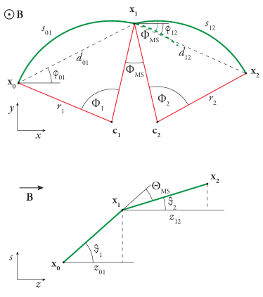
Figure 1: Particle trajectory in a homogeneous magnetic field defined by a triplet of hits $\mathbf{x_{0}}$, $\mathbf{x_{1}}$ and $\mathbf{x_{2}}$, with particle scattering at $\mathbf{x_{1}}$. The top view shows the projection to the plane transverse to the magnetic field, whereas the bottom view is a projection to the field axis-arclength ($s$) plane. $r_{1}$ and $r_{2}$ are the transverse track radii before and after the scattering process, $s_{01}$ and $s_{12}$ the corresponding arclengths and $\Phi_{1}$ and $\Phi_{2}$ the bending angles. $d_{01}$ and $d_{12}$ denote the transverse distances between $\mathbf{x_{0}}$ and $\mathbf{x_{1}}$, and $\mathbf{x_{1}}$ and $\mathbf{x_{2}}$, respectively. The azimuthal angles of the corresponding distance vectors are labeled $\varphi_{01}$ and $\varphi_{12}$ and $\Phi_{MS}$ is the transverse scattering angle. In the longitudinal plane, $z_{01}$ and $z_{02}$ denote the distances between the measurement points along the field axis, $\vartheta_{1}$ and $\vartheta_{2}$ are the polar angles of the arcs and $\Theta_{MS}$ is the longitudinal scattering angle.

The basic unit of the track fit is a triplet of hits in successive detector layers. In the absence of MS and energy losses, the description of a helix through three points requires eight parameters, namely a starting point (three parameters), an initial direction (two parameters), the curvature (one parameter) and the distances to the second and third point (two parameters). MS in the central plane requires two additional parameters to describe the change in track direction. Three space points, which we assume to be measured without uncertainties, do however only provide a total of nine coordinates; additional constraints are thus needed to obtain the track parameters and scattering angles. These constraints can be obtained from MS theory since the scattering angles depend statistically on the particle type and momentum, and the material of the detector.

Starting from a hit triplet, see Figure 1, a trajectory consisting of two arcs connecting the three-dimensional space points is constructed. It is assumed that the middle point $\mathbf{x_{1}}$ lies in a scattering plane which deflects the particle and thus creates a kink in the trajectory. The corresponding scattering angles in the transverse and longitudinal plane are denoted by $\Phi_{MS}$ and $\Theta_{MS}$ respectively.

We assume that the particle momentum (and thus its three-dimensional radius $R_{3D}$) is conserved. The scattering angles $\Phi_{MS}$ and $\Theta_{MS}$ have a mean of zero and variances $\sigma_{\vartheta}^{2}=\sigma_{MS}^{2}$ and $\sigma_{\phi}^{2}=\sigma_{MS}^{2}/\sin^{2}\vartheta$, which can be calculated from MS theory, using e.g. the Highland approximation [10]. The task is thus to find a unique $R_{3D}$ which minimizes the scattering angles, explicitly the following $\chi^{2}$ function:

$$\chi^{2}(R_{3D})=\frac{\Phi_{MS}(R_{3D})^{2}}{\sigma_{\phi}^{2}}+\frac{\Theta_{MS}(R_{3D})^{2}}{\sigma_{\vartheta}^{2}}\ .$$ (1)

For weak MS effects the momentum dependence of the scattering uncertainty is negligible; the case of large MS effects is discussed in more detail in section 2.4. Assuming $\frac{d\sigma_{MS}}{dR_{3D}}=0$, the minimization of $\chi^{2}(R_{3D})$ is thus equivalent to solving the equation

$$\sin^{2}\vartheta\;\frac{d\Phi_{MS}(R_{3D})}{dR_{3D}}\;\Phi_{MS}(R_{3D})\;+\;\frac{d\Theta_{MS}(R_{3D})}{dR_{3D}}\;\Theta_{MS}(R_{3D})=0$$ (2)

for $R_{3D}$. The scattering angle in the transverse plane $\Phi_{MS}$ is given by

$$\Phi_{MS}=(\varphi_{12}-\varphi_{01})-\frac{\Phi_{1}(R_{3D})+\Phi_{2}(R_{3D})}{2}\ ,$$ (3)

where the bending angles $\Phi_{1}$ and $\Phi_{2}$ are the solutions of the transcendent equations

$$\sin^{2}\frac{\Phi_{1}}{2} =\frac{d_{01}^{2}}{4R_{3D}^{2}}+\frac{z_{01}^{2}}{R_{3D}^{2}}\frac{\sin^{2}\frac{\Phi_{1}}{2}}{\Phi_{1}^{2}}\ ,$$

$$\sin^{2}\frac{\Phi_{2}}{2} =\frac{d_{12}^{2}}{4R_{3D}^{2}}+\frac{z_{12}^{2}}{R_{3D}^{2}}\frac{\sin^{2}\frac{\Phi_{2}}{2}}{\Phi_{2}^{2}}\ .$$ (4)

These equations have several solutions depending on the number of half-turns of the track. However, for most practical cases it is sufficient to consider the first two solutions.

Similarly, the scattering angle in the longitudinal plane is given by

$$\Theta_{MS}=\vartheta_{2}-\vartheta_{1}$$ (5)

where the polar angles $\vartheta_{1}$ and $\vartheta_{2}$ can be calculated from the azimuthal bending angles using the relations

$$\sin\vartheta_{1} =\frac{d_{01}}{2R_{3D}}\mathrm{cosec}\left(\frac{z_{01}}{2R_{3D}\cos\vartheta_{1}}\right)\ ,$$

$$\sin\vartheta_{2} =\frac{d_{12}}{2R_{3D}}\mathrm{cosec}\left(\frac{z_{12}}{2R_{3D}\cos\vartheta_{2}}\right)\ .$$ (6)

Alternatively the relations

$$\Phi_{1} =\frac{z_{01}}{R_{3D}\cos\vartheta_{1}}\ ,$$

$$\Phi_{2} =\frac{z_{12}}{R_{3D}\cos\vartheta_{2}}$$ (7)

between the azimuthal bending angles and the polar angles can be exploited.

Equations 4 and 6 have no algebraic solutions; they can either be solved by numerical iteration or by using a linearization around an approximate solution; the second approach is discussed in the following.

2.1 Taylor expansion around the circle solution

The circle solution describes the case of constant curvature in the plane transverse to the magnetic field $r_{1}=r_{2}$ and no scattering in that plane, $\Phi_{MS}=0$. This solution exists for any hit triplet and is thus a good starting point for the linearization. The radius $R_{C}$ of the circle in the transverse plane going through three points is given by

$$R_{C}=\frac{d_{01}\;d_{12}\;d_{02}}{2\;[(\mathbf{x_{1}}-\mathbf{x_{0}})\times(\mathbf{x_{2}}-\mathbf{x_{1}})]_{z}},$$ (8)

where $d_{ij}$ is the transverse distance between the hits $i$ and $j$ of the triplet, see Figure 1.

The bending angles for the circle solution are

$$\Phi_{1C} =2\arcsin\frac{d_{01}}{2R_{C}}\ ,$$

$$\Phi_{2C} =2\arcsin\frac{d_{12}}{2R_{C}}\ .$$ (9)

Note that the above equations have in general two solutions ($\Phi_{iC}<\pi$ and $\Phi_{iC}>\pi$) and care is needed to select the physical one, especially for highly bent tracks. The corresponding three-dimensional radii of the arcs are calculated as

$$R_{3D,1C}^{2} =R_{C}^{2}+\frac{z_{01}^{2}}{\Phi_{1C}^{2}}\ ,$$

$$R_{3D,2C}^{2} =R_{C}^{2}+\frac{z_{12}^{2}}{\Phi_{2C}^{2}}\ .$$ (10)

In general $\Theta_{MS}\neq 0$ such that the two radii are not identical. Using equation 7, polar angles for the circle solution are obtained:

$$\vartheta_{1C} =\arccos\frac{z_{01}}{\Phi_{1C}R_{3D,1C}}\ ,$$

$$\vartheta_{2C} =\arccos\frac{z_{12}}{\Phi_{2C}R_{3D,2C}}\ .$$ (11)

Starting from this special circle solution with no scattering in the transverse plane, we calculate the general solution $\Phi_{MS}\neq 0$ which minimizes equation 1 and for which momentum conservation is fulfilled, i.e. $R_{3D}$ does not change between the segments. With the positions of the three hits given, the arc lengths and the polar angles depend only on the radius, i.e. $\Phi_{1,2}=\Phi_{1,2}(R_{3D})$ and $\vartheta_{1,2}=\vartheta_{1,2}(R_{3D})$ (equations 4 and 6). We can therefore perform a Taylor expansion to first order around the circle solution which is described by the parameters $R_{3D,1C}$, $R_{3D,2C}$, $\Phi_{1C}$, $\Phi_{2C}$, $\vartheta_{1C}$ and $\vartheta_{2C}$:

$$\Phi_{1}(R_{3D}) \approx\Phi_{1C}+(R_{3D}-R_{3D,1C})\left.\frac{\operatorname{d}\!\Phi_{1}}{\operatorname{d}\!R_{3D}}\right|_{\Phi_{1C}},$$

$$\Phi_{2}(R_{3D}) \approx\Phi_{2C}+(R_{3D}-R_{3D,2C})\left.\frac{\operatorname{d}\!\Phi_{2}}{\operatorname{d}\!R_{3D}}\right|_{\Phi_{2C}}$$ (12)

and

$$\vartheta_{1}(R_{3D}) \approx\vartheta_{1C}+(R_{3D}-R_{3D,1C})\left.\frac{\operatorname{d}\!\vartheta_{1}}{\operatorname{d}\!R_{3D}}\right|_{\vartheta_{1C}}\ ,$$

$$\vartheta_{2}(R_{3D}) \approx\vartheta_{2C}+(R_{3D}-R_{3D,2C})\left.\frac{\operatorname{d}\!\vartheta_{2}}{\operatorname{d}\!R_{3D}}\right|_{\vartheta_{2C}}\ .$$ (13)

The derivatives $\left.\frac{\operatorname{d}\!\Phi_{1}}{\operatorname{d}\!R_{3D}}\right|_{\Phi_{1C}}$ and $\left.\frac{\operatorname{d}\!\Phi_{2}}{\operatorname{d}\!R_{3D}}\right|_{\Phi_{2C}}$ can be represented by index parameters:

$$\left.\frac{\operatorname{d}\!\Phi_{1}}{\operatorname{d}\!R_{3D}}\right|_{\Phi_{1C}} =-\alpha_{1}\frac{\Phi_{1C}}{R_{3D,1C}}\ ,$$

$$\left.\frac{\operatorname{d}\!\Phi_{2}}{\operatorname{d}\!R_{3D}}\right|_{\Phi_{2C}} =-\alpha_{2}\frac{\Phi_{2C}}{R_{3D,2C}}\ ,$$ (14)

which are calculated from equation 4 as

$$\alpha_{1} =\frac{R_{C}^{2}\Phi_{1C}^{2}+z_{01}^{2}}{\frac{1}{2}R_{C}^{2}\Phi_{1C}^{3}\cot\frac{\Phi_{1C}}{2}+z_{01}^{2}}\ ,$$

$$\alpha_{2} =\frac{R_{C}^{2}\Phi_{2C}^{2}+z_{12}^{2}}{\frac{1}{2}R_{C}^{2}\Phi_{2C}^{3}\cot\frac{\Phi_{2C}}{2}+z_{12}^{2}}\ .$$ (15)

The derivatives of the polar angles are obtained from equation 6 and can be expressed by the same index parameters:

$$\left.\frac{\operatorname{d}\!\vartheta_{1}}{\operatorname{d}\!R_{3D}}\right|_{\vartheta_{1C}}=\frac{\cot\vartheta_{1C}}{R_{3D,1C}}(1-\alpha_{1}),$$

$$\left.\frac{\operatorname{d}\!\vartheta_{2}}{\operatorname{d}\!R_{3D}}\right|_{\vartheta_{2C}}=\frac{\cot\vartheta_{2C}}{R_{3D,2C}}(1-\alpha_{2}).$$ (16)

2.2 Linearization of the scattering angles

The above relations can now be used to calculate a linearized expression for the MS angles. For $\Phi_{MS}$ we obtain:

$$\Phi_{MS} =\varphi_{12}-\varphi_{01}-\frac{\Phi_{1}(R_{3D})}{2}-\frac{\Phi_{2}(R_{3D})}{2}$$

$$=\tilde{\Phi}+{\eta}\;R_{3D}\ ,$$ (17)

where we have introduced two new parameters:

$$\tilde{\Phi} =-\frac{1}{2}(\Phi_{1C}\alpha_{1}+\Phi_{2C}\alpha_{2})\ ,$$ (18)

$${\eta} =\frac{\operatorname{d}\!\Phi_{MS}}{\operatorname{d}\!R_{3D}}=\frac{\Phi_{1C}\;\alpha_{1}}{2R_{3D,1C}}+\frac{\Phi_{2C}\;\alpha_{2}}{2R_{3D,2C}}\ .$$ (19)

And similarly for the polar angle $\Theta_{MS}$ we obtain:

$$\Theta_{MS} =\vartheta_{2}-\vartheta_{1}$$

$$=\tilde{\Theta}+{\beta}\;R_{3D}\ ,$$ (20)

with the new parameters

$$\tilde{\Theta} =\vartheta_{2C}-\vartheta_{1C}-\Bigl{(}\left(1-\alpha_{2}\right)\cot\vartheta_{2C}-\left(1-\alpha_{1}\right)\cot\vartheta_{1C}\Bigr{)}\ ,$$ (21)

$${\beta} =\frac{\operatorname{d}\!\Theta_{MS}}{\operatorname{d}\!R_{3D}}=\frac{(1-\alpha_{2})\cot\vartheta_{2C}}{R_{3D,2C}}-\frac{(1-\alpha_{1})\cot\vartheta_{1C}}{R_{3D,1C}}\ .$$ (22)

2.3 Linearized triplet track fit

We can now minimize the $\chi^{2}$-function by inserting the derivatives and the expressions for the scattering angles obtained from the linearization in equation 2. For the three-dimensional radius we obtain

$$R_{3D}^{min}=-\frac{{\eta}\;\tilde{\Phi}\;\sin^{2}\vartheta+{\beta}\;\tilde{\Theta}}{{\eta}^{2}\sin^{2}\vartheta+{\beta}^{2}}\ .$$ (23)

Here is $\vartheta$ the polar angle at the scattering layer, which can be taken as the average of $\vartheta_{1C}$ and $\vartheta_{2C}$. The minimum $\chi^{2}$ value is

$$\chi^{2}_{min}=\frac{1}{\sigma_{MS}^{2}}\frac{({\beta}\;\tilde{\Phi}-{\eta}\;\tilde{\Theta})^{2}}{{\eta}^{2}+{\beta}^{2}/\sin^{2}\vartheta}$$ (24)

and for the uncertainty of the three-dimensional radius we get

$$\sigma(R_{3D})=\sigma_{MS}\sqrt{\frac{1}{{\eta}^{2}\sin^{2}\vartheta+{\beta}^{2}}}\ .$$ (25)

The scattering angles are finally given by:

$$\Phi_{MS} ={\beta}\ \frac{{\beta}\;\tilde{\Phi}-{\eta}\;\tilde{\Theta}}{{\eta}^{2}\sin^{2}\vartheta+{\beta}^{2}}\ ,$$ (26)

$$\Theta_{MS} =-{\eta}\sin^{2}\vartheta\ \frac{{\beta}\;\tilde{\Phi}-{\eta}\;\tilde{\Theta}}{{\eta}^{2}\sin^{2}\vartheta+{\beta}^{2}}\ .$$ (27)

It is straight-forward to calculate further track parameters using the linearization described above.

Note that in this approach the fitted track parameters are independent of the momentum and the MS uncertainty. The latter can be calculated after fitting the track parameters which allows for an elegant treatment of the material effects. We have thus obtained a non-iterative solution to the triplet problem with multiple scattering.

2.4 Strong Multiple Scattering and Weak Bending

The regime where the MS uncertainty is of similar size as the sum of the bending angles, $\sigma_{MS}\approx\Phi_{1}+\Phi_{2}$, we define as strong MS or weak bending. This corresponds to cases with either a large amount of material at the scattering layer or weak magnetic field strength. In this regime the momentum dependence of the scattering uncertainty leads to a systematic shift (bias) of the fitted radius towards larger values. This bias can be compensated by including the momentum dependence in the minimization of the $\chi^{2}$ function, given in equation 1, using the ansatz $\sigma_{MS}=b/R_{3D}$ which is motivated by the Highland formula [10]. Here $b$ is an effective scattering parameter which is approximately given by

$$b\approx\frac{4.5~{}\textrm{cm T}}{B}\;\sqrt{X/X_{0}}$$ (28)

and assumed to vary only weakly within the parameter range of the fit. The so obtained unbiased result

$$R_{3D}^{unbiased}=-\;\frac{{\eta}\;\tilde{\Phi}\;\sin^{2}{\vartheta}+{\beta}\;\tilde{\Theta}}{{\eta}^{2}\;\sin^{2}{\vartheta}+{\beta}^{2}}\ \left(\frac{3}{4}+\;\frac{\sqrt{1-8\;\delta^{2}\sin^{2}{\vartheta}}}{4}\right)$$ (29)

with

$$\delta=\frac{{\beta}\;\tilde{\Phi}-{\eta}\;\tilde{\Theta}}{{\eta}\;\tilde{\Phi}\;\sin^{2}{\vartheta}+{\beta}\;\tilde{\Theta}}$$ (30)

has only a solution if

$$8\;\delta^{2}\sin^{2}{\vartheta}\leq 1\ .$$ (31)

For small bias parameters, $\delta\approx 0$, equation 23 is restored. The bias parameter $\delta$ is just given by the hit triplet geometry but it can also be expressed by fitted parameters:

$$\delta^{2}\sin^{2}{\vartheta}\ =\ \frac{\sigma(R_{3D}^{min})^{2}}{{R_{3D}^{min}}^{2}}\;\chi^{2}_{min}$$ (32)

using equations 23, 24 and 25. The bias term is thus proportional to the sum of the squared scattering angles:

$$\delta^{2}\sin^{2}{\vartheta}\ \propto\ \Phi_{MS}^{2}+\Theta_{MS}^{2}\sin^{2}{\vartheta}\ .$$ (33)

From equation 31 a condition on the minimum significance for the radius measurement can be derived:

$$\frac{R_{3D}}{\sigma(R_{3D})}>\sqrt{8\;\chi^{2}}\ .$$ (34)

If the radius significance is not large enough, $\frac{R_{3D}}{\sigma(R_{3D})}\lesssim 10$, significant bias corrections apply.

For small bending angles (weak bending region!) the relation $|{\beta}|\ll|{\eta}|$ holds and the relative resolution of the three-dimensional radius (momentum) is approximately given by

$$\frac{\sigma(R_{3D})}{R_{3D}}=\frac{\sigma(p)}{p}=\frac{2\;b}{s}\ .$$ (35)

We can then rewrite equation 34 as

$$s^{2}>32\;b^{2}\chi^{2}$$ (36)

where $s=s_{01}+s_{12}$ defines the length of the triplet trajectory. This relation should be respected, for example in the design of detectors, to allow for a decent momentum measurement.

2.5 Example Spectrometer

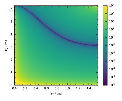
Figure 2: Relative momentum resolution for the example spectrometer with the MS triplet fit, see equation 37, as a function of the bending angle $\Phi_{2}$ and the polar angle $\vartheta_{2}$.

The resolution of the triplet track fit is investigated for a simple spectrometer configuration with three detector layers for which the spatial hit uncertainties are negligible. The first two layers are spaced closely together and the third layer is placed further apart, i.e. we assume $\Phi_{1}\ll\Phi_{2}$ for the sweep angles defined in Figure 1. The relative momentum resolution is then calculated using the previously derived expressions for the fitted radius and associated variances as follows:

$$\frac{\sigma_{R_{3D}}}{{R_{3D}}}=2\;\sigma_{MS}\;\left(\Phi_{2}^{2}\alpha_{2}^{2}\;\sin^{2}\vartheta_{2}\;+\;4(1-\alpha_{2})^{2}\;\cot^{2}\vartheta_{2}\right)^{-\frac{1}{2}},$$ (37)

with $\alpha_{2}$ given by:

$$\alpha_{2}^{-1} = \cos^{2}{\vartheta_{2}}\;+\;\frac{\Phi_{2}}{2}\cot{\left(\frac{\Phi_{2}}{2}\right)}\;\sin^{2}{\vartheta_{2}}\ .$$ (38)

The resulting resolution as a function of $\Phi_{2}$ and $\vartheta_{2}$ is shown in figure 2. Note that for some special cases, if $1/\alpha_{2}\rightarrow 0$, the momentum resolution approaches zero. For transverse going tracks ($\vartheta_{2}=\pi/2$) this is the case if $\Phi_{2}=\pi$ (i.e. semi-circles). The geometry of track detectors in a regime where MS dominates can thus be optimized for an almost perfect measurement at certain specific momenta.

3 Combining Triplets

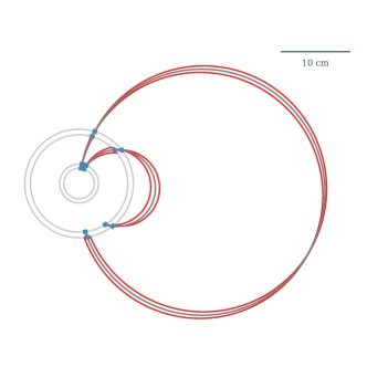
Figure 3: Simulated Mu3e tracker geometry in the transverse plane. Two undisturbed example trajectories with a momentum of $53\text{\,}\mathrm{M}\mathrm{eV}\mathrm{/}{c}$ and $16.5\text{\,}\mathrm{M}\mathrm{eV}\mathrm{/}{c}$ and a fixed polar angle of $\vartheta=$90\text{\,}\mathrm{\SIUnitSymbolDegree}$$ are shown. The red lines indicate the uncertainties induced by scattering in the previous layer for a particle moving outwards. The blue marks indicate the measurement uncertainties. All uncertainties are artificially increased by a factor five to enhance the visibility. A magnetic field of $1\text{\,}\mathrm{T}$ is assumed.

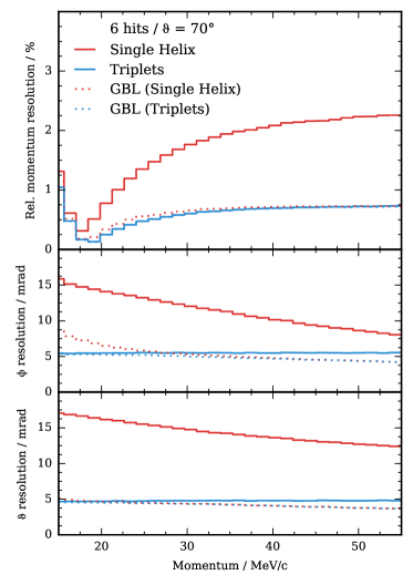
Figure 4: Track parameter resolution for the Mu3e geometry, described in Figure 3, for different track fits as a function of the track momentum. The top panel shows the relative momentum resolution and the bottom panels show the resolution for the azimuthal angle $\phi$ and the polar angle $\vartheta$ for tracks with a polar angle of $70\text{\,}\mathrm{\SIUnitSymbolDegree}$. The resolutions are calculated as the RMS of the parameter residual distributions for each bin.

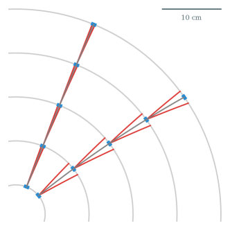
Figure 5: Simulated generic pixel tracker geometry with associated uncertainties in the transverse plane. Two undisturbed example trajectories are shown with momenta of $5\text{\,}\mathrm{G}\mathrm{eV}\mathrm{/}{c}$ (upper) and $1\text{\,}\mathrm{G}\mathrm{eV}\mathrm{/}{c}$ (lower) and a fixed polar angle of $\vartheta=$70\text{\,}\mathrm{\SIUnitSymbolDegree}$$. The uncertainties, see Figure 3 for explanations, have a scaling factor of one-hundred. A magnetic field of $2\text{\,}\mathrm{T}$ is assumed.

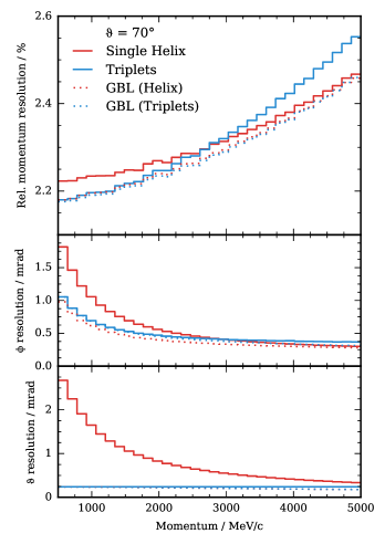
Figure 6: Track parameter resolution for the equidistant layer geometry, described in Figure 5, for different track fits as a function of the track momentum. The top panel shows the relative momentum resolution and the bottom panels show the resolution of the azimuthal angle $\phi$ and the polar angle $\vartheta$ for tracks with a polar angle of $70\text{\,}\mathrm{\SIUnitSymbolDegree}$. The resolutions are calculated as the RMS of the parameter residual distributions for each bin.

Several triplets can be combined to form longer tracks. As MS in each sensor layer is independent of all other layers the following global $\chi^{2}$ function is minimized:

$$\chi_{global}^{2}=\sum_{i}^{n_{hit}-2}\chi^{2}_{i}\ ,$$ (39)

where $\chi_{i}$ is the minimization function for the $i$-th triplet number previously defined in equation 1. The total number of triplets is given by $n_{hit}-2$. The minimization of equation 39 is equivalent to a weighted average of the resulting radii $R_{3D,i}$ of the individual fits:

$$\overline{R_{3D}}=\sum_{i}^{n_{hit}-2}\frac{R_{3D,i}^{3}}{\sigma(R_{3D,i})^{2}}/\sum_{i}^{n_{hit}-2}\frac{R_{3D,i}^{2}}{\sigma(R_{3D,i})^{2}}\ .$$ (40)

with the corresponding uncertainty given by

$$\sigma(\overline{R_{3D}})=\frac{\overline{R_{3D}}}{\sqrt{\sum_{i}^{n_{hit}-2}\frac{R_{3D,i}^{2}}{\sigma(R_{3D,i})^{2}}}}\ .$$ (41)

This averaging formula is free of any bias if unbiased three-dimensional radii from equation 29 are used as input and if $\frac{\sigma(R_{3D,i})}{R_{3D,i}}$ is constant, which is a very good assumption for most cases.

Fitting of multiple hits, $n_{hit}>3$, is performed in a three step procedure: first all triplets of consecutive hits are fitted individually, second a weighted mean of the three-dimensional track radii is calculated which is then used in the third step to recalculate all other track parameters. It is worth to note that the expected variance of the MS angle for each triplet only enters at the averaging step, where it can be calculated to very good accuracy from the locally fitted triplet track parameters. Effects from energy loss can also be incorporated at this step.

We can now use the average radius $\overline{R_{3D}}$ together with our linearization to obtain globally fitted (updated) values for the sweep angles $\Phi_{i}$ and the polar angles $\vartheta_{i}$:

$$\Phi_{i}^{\prime} =\Phi_{i}-(\overline{R_{3D}}-R_{3D,i})\;\frac{\Phi_{i}}{R_{3D,i}}\;\alpha_{i}\ ,$$ (42)

$$\vartheta_{i}^{\prime} =\vartheta_{i}-(\overline{R_{3D}}-R_{3D,i})\;\frac{\cot\vartheta_{i}}{R_{3D,i}}\;(1-\alpha_{i})\ .$$ (43)

Alternatively, $\vartheta_{i}^{\prime}$ can also be obtained from the relation

$$\vartheta_{i}^{\prime}=\arccos\frac{{\eta}\;z_{\{i-1,i\}}}{\overline{R_{3D}}\;\Phi_{i}^{\prime}}$$ (44)

if the sweep angle is known.

We have thus obtained a non-iterative solution to the MS problem which is especially suitable for implementation on massively parallel architectures such as graphics processors (GPUs) as the triplets can be fit in parallel.

4 Track Fit Comparisons

To compare the performance of the triplets fit with other fit algorithms we simulate particle tracks in different detector geometries using a toy Monte Carlo. Tracks are then reconstructed using the triplets fit, a single helix fit [1], and the general broken lines (GBL) fit [7].

For the comparison study we choose two exemplary geometries. Detector layers are modeled as cylindrical high resolution pixel sensors centered around the origin and aligned along the direction of the homogeneous magnetic field. Tracks are generated at the origin and propagated in the magnetic field to the detector layers. MS is simulated by smearing the track direction at each layer with kink angles drawn from a Gaussian distribution with a width according to the Highland formula [10, 11]. The position resolution of the detector is simulated by smearing the registered hit positions with a Gaussian distribution along both sensitive directions.

The triplets fit, which includes only MS uncertainties, is performed as described in the previous section.

The single helix fit, which is another example for a direct track fit, only takes into account the spatial measurement uncertainties. Here, the transverse track parameters are obtained from the Karimäki circle fit [1] and the longitudinal parameters result from a linear regression to the points in the projected arclength-$z$ plane.

The GBL fit is an extended track fit that takes into account both, scattering effects and spatial uncertainties. It has been shown [7] to be equivalent to the Kálmán filter [3] and uses a track model consistent with all simulated uncertainties.

The GBL algorithm performs a linearized fit by varying positions and kink angles at selected points around a reference trajectory. This reference can be derived from any direct track fit. Here, we use the helix fit and the triplets fit for comparison. In the first case, the track parameters are refitted by introducing non-vanishing kink angles. In the second case, the kink angles are optimized by introducing residuals to the measured positions. In this study we use only one iteration and ideally, the GBL converges to the same optimized trajectory from either of the two initial estimates in that single step.

For the comparison study, the fitted track parameters are calculated at the inner-most detector layer at which the track parameters are maximally uncorrelated.

The first simulated configuration is the silicon pixel tracker of the Mu3e experiment [8]. The geometry and example trajectories to illustrate the uncertainties are shown in figure 3. The detector is placed in a homogeneous magnetic field of $B=$1\text{\,}\mathrm{T}$$, has four layers with radii at approximately $2.2\text{\,}\mathrm{cm}2.8\text{\,}\mathrm{cm}7.0\text{\,}\mathrm{cm}7.8\text{\,}\mathrm{cm}$, and is optimized for low momentum electrons in a momentum range of $15\text{\,}\mathrm{M}\mathrm{eV}\mathrm{/}{c}53\text{\,}\mathrm{M}\mathrm{eV}\mathrm{/}{c}$. The spatial resolution on the detector plane is $80/\sqrt{12}$ $\text{\,}\mathrm{\SIUnitSymbolMicro m}$ and the layer thickness is $0.1\text{\,}\mathrm{\char 37\relax}$ radiation lengths.

The resulting parameter resolution for the four different fits is shown in figure 4. The triplets fit has a consistently better resolution than the single helix fit in all track parameters. The GBL-fit with the triplets as reference (GBL-T) shows no significant improvement at very small momentum ($\lesssim$$25\text{\,}\mathrm{M}\mathrm{eV}\mathrm{/}{c}$). In this region MS uncertainties dominate the track uncertainties. Above $25\text{\,}\mathrm{M}\mathrm{eV}\mathrm{/}{c}$ the GBL-T fit allows for small improvements of the angular resolutions as spatial uncertainties start to contribute.

The GBL-fit with the single helix reference (GBL-H) reproduces for $\gtrsim$$30\text{\,}\mathrm{M}\mathrm{eV}\mathrm{/}{c}$ the result of GBL-T. Although GBL-H improves with respect to the single helix reference fit also for $\lesssim$$30\text{\,}\mathrm{M}\mathrm{eV}\mathrm{/}{c}$, the momentum and azimuthal angle resolution is worse than for triplets fit and GBL-T. In this region the single helix parameterization is not a good reference and linearization point for the GBL. With the large non-linearity of the strongly curved tracks the single GBL-H step is insufficient.

The behaviour of the position resolution (not shown) follows the behaviour of the angle resolution, i.e. the GBL is slightly better than the triplets fit and the helix fit is significantly worse than other fits.

To extend this study beyond the unique Mu3e configuration, a generic pixel tracker design similar to existing or planned trackers for high-energy collider detectors, e.g. ATLAS, CMS or ILC, is evaluated. It comprises five equidistant detector layers at radii between $40\text{\,}\mathrm{mm}340\text{\,}\mathrm{mm}$ with a spatial resolution of $50/\sqrt{12}$ $\text{\,}\mathrm{\SIUnitSymbolMicro m}$ and a sensor thickness corresponding to $2\text{\,}\mathrm{\char 37\relax}$ of radiation length. Particles are simulated in the momentum range between $500\text{\,}\mathrm{M}\mathrm{eV}\mathrm{/}{c}5000\text{\,}\mathrm{M}\mathrm{eV}\mathrm{/}{c}$, a region where MS significantly contributes to the track uncertainties.

The track parameter resolution of the four algorithms is shown in figure 6. All fits show a similar momentum resolution. At low momentum the triplets fit provides the better resolution, at higher momentum the single helix fit, with a crossover at around $3000\text{\,}\mathrm{M}\mathrm{eV}\mathrm{/}{c}$. The GBL-fits give the optimal resolution over the full range.

The polar angle resolution of the triplets fit is constant, its value fully determined by the spatial hit uncertainties. Interestingly, the triplets fit gives a significantly better resolution than the single helix fit even at high momenta. For the GBL-fits an improvement of the polar angle resolution for $\gtrsim$$3000\text{\,}\mathrm{M}\mathrm{eV}\mathrm{/}{c}$ is visible.

The azimuthal angle resolution shows a similar crossover behaviour as the momentum resolution at about $3000\text{\,}\mathrm{M}\mathrm{eV}\mathrm{/}{c}$. Again both GBL-fits lead to an improvement of the resolution. But they show a small difference at low momentum. Interestingly, the first iteration step of GBL-H yields a better azimuthal resolution than GBL-T. Note that the position of the crossover point depends on the geometry, the material, and the spatial resolution of the detector.

We have compared execution times and the number of floating point operations for several implementations of the triplets fit and the single helix fit. The number of cycles required varies greatly depending on how many geometric quantities are pre-calculated and cached and whether (and where) a covariance matrix is calculated. With ideal caching and no calculation of the covariance matrix, the triplets fit outperforms the single helix fit by almost a factor of 2; if all track parameters and the full covariance matrix is calculated at each hit position, the single helix fit (with its global covariance matrix) needs about a factor 2 (5) less cycles for three (eight) hits.

5 Conclusions

We presented a new track fit algorithm, the triplets fit, that is only based on MS uncertainties to determine global momentum and local direction parameters. The triplets fit is motivated by the excellent position resolution of modern silicon pixel sensors which create track fitting problems with dominating MS uncertainties.

Although developed initially for reconstructing very low momentum electrons in the Mu3e experiment the triplets fit exhibits good performance for pixel trackers at the high energy experiments at LHC where MS uncertainties dominate or significantly contribute up to around $10\text{\,}\mathrm{G}\mathrm{eV}\mathrm{/}{c}$. In this regime, the performance of the triplets fit is as good as for GBL-fits.

The triplets fit enables a very fast computation of track parameters and provides a natural scheme for track finding and linking via the combination of single triplets. This makes the triplets fit ideally suited for fast online reconstruction, as a reference for extended track fits, and as fast algorithm for pattern recognition problems.

References

-
[1]
V. Karimäki,
Effective
circle fitting for particle trajectories, Nucl. Instr. Meth. A 305 (1)
(1991) 187–191.
doi:10.1016/0168-9002(91)90533-V.
URL http://www.sciencedirect.com/science/article/pii/016890029190533V -
[2]
R. E. Kalman,
A
new approach to linear filtering and prediction problems, J. Basic Eng.
82 (1) (1960) 35.
doi:10.1115/1.3662552.
URL http://FluidsEngineering.asmedigitalcollection.asme.org/article.aspx?articleid=1430402 -
[3]
R. Frühwirth,
Application
of Kalman filtering to track and vertex fitting, Nucl. Instr. Meth. A
262 (2–3) (1987) 444–450.
doi:10.1016/0168-9002(87)90887-4.
URL http://www.sciencedirect.com/science/article/pii/0168900287908874 -
[4]
P. Billoir, S. Qian,
Simultaneous
pattern recognition and track fitting by the Kalman filtering method, Nucl.
Instr. Meth. A 294 (1–2) (1990) 219–228.
doi:10.1016/0168-9002(90)91835-Y.
URL http://www.sciencedirect.com/science/article/pii/016890029091835Y - [5] V. Blobel, A new fast track-fit algorithm based on broken lines, Nucl. Instr. Meth. A 566 (2006) 14–17.
-
[6]
V. Blobel, C. Kleinwort, F. Meier,
Fast
alignment of a complex tracking detector using advanced track models,
Comput. Phys. Commun. 182 (9) (2011) 1760–1763.
doi:10.1016/j.cpc.2011.03.017.
URL http://www.sciencedirect.com/science/article/pii/S0010465511001093 -
[7]
C. Kleinwort,
General
broken lines as advanced track fitting method, Nucl. Instr. Meth. A 673
(2012) 107–110.
doi:10.1016/j.nima.2012.01.024.
URL http://www.sciencedirect.com/science/article/pii/S0168900212000642 -
[8]
N. Berger, et al.,
A
tracker for the Mu3e experiment based on high-voltage monolithic active pixel
sensors, Nucl. Instr. Meth. A 732 (2013) 61–65.
doi:10.1016/j.nima.2013.05.035.
URL http://www.sciencedirect.com/science/article/pii/S016890021300613X -
[9]
A. Blondel, et al., Research proposal for
an experiment to search for the decay {mu}
- eee, ArXiv13016113 Hep-Ex Physicsphysics.
URL http://arxiv.org/abs/1301.6113 -
[10]
V. L. Highland,
Some
practical remarks on multiple scattering, Nucl. Instr. Meth. A 129 (2)
(1975) 497–499.
doi:10.1016/0029-554X(75)90743-0.
URL http://www.sciencedirect.com/science/article/pii/0029554X75907430 -
[11]
K. A. Olive, et al.,
Review of particle
physics, Chin.Phys. C38 (2014) 090001.
doi:10.1088/1674-1137/38/9/090001,\%002010.1088/1674-1137/38/9/090001.
URL http://inspirehep.net/record/1315584/export/hx