Logarithmic Time One-Against-Some

Abstract

We create a new online reduction of multiclass classification to binary classification for which training and prediction time scale logarithmically with the number of classes. We show that several simple techniques give rise to an algorithm that can compete with one-against-all in both space and predictive power while offering exponential improvements in speed when the number of classes is large.

1 Introduction

Can we effectively predict one of $K$ classes in polylogarithmic time in $K$? This question gives rise to the area of extreme multiclass classification [1, 3, 4, 8, 18, 20, 27], in which $K$ is very large. If efficiency is not a concern, the most common and generally effective representation for multiclass prediction is a one-against-all (OAA) structure. Here, inference consists of computing a score for each class and returning the class with the maximum score. An attractive strategy for picking one of $K$ items efficiently is to use a tree; unfortunately, this often comes at the cost of increased error.

A general replacement for the one-against-all approach must satisfy a difficult set of desiderata.

• High accuracy: The approach should provide accuracy competitive with OAA, a remarkably strong baseline[21] which is the standard “output layer” of many learning systems such as winners of the ImageNet contest [12, 23].

• High speed at training time and test time: A multiclass classifier must spend at least $\Omega(\log K)$ time [8]) so this is a natural benchmark to optimize against.

• Online operation: Many learning algorithms use either online updates or mini-batch updates. Approaches satisfying this constraint can be easily composed into an end-to-end learning system for solving complex problems like image recognition. For algorithms which operate in batch fashion, online components can be easily used.

• Linear space: In order to have a drop-in replacement for OAA, an approach must not take much more space than OAA. Memory is at a premium when $K$ is very large, especially for models trained on GPUs, or deployed to small devices.

We use an OAA-like structure to make a final prediction, but instead of scoring every class, we only score a small subset of $O(\log K)$ classes. We call this “one-against-some” (OAS). How can you efficiently determine what classes should be scored? We use a dynamically built tree to efficiently whittle down the set of candidate classes. The goal of the tree is to maximize the recall of the candidate set so we call this approach “The Recall Tree.”

Figure 1 depicts the inference procedure for the Recall Tree: an example is routed through a tree until termination, and then the set of eligible classes compete to predict the label. We use this inference procedure at training time, to facilitate end-to-end joint optimization of the predictors at each internal node in the tree (the “routers”), the tree structure, and the final OAS predictors.

The Recall Tree achieves good accuracy, improving on previous online approaches [8] and sometimes surpassing the OAA baseline. The algorithm requires only $\mathrm{poly}(\log K)$ time during training and testing. In practice, the computational benefits are substantial when $K\geq 1000$. The Recall Tree constructs a tree and learns parameters in a fully online manner as a reduction allowing composition with systems trained via online updates. All of this requires only a factor of 2 more space than OAA approaches.

Our contributions are the following:

• We propose a new online tree construction algorithm which jointly optimizes the construction of the tree, the routers and the underlying OAS predictors (see section 3.1).

• We analyze elements of the algorithm, including a new boosting bound (see section 3.3) on multiclass classification performance and a representational trick which allows the algorithm to perform well if either a tree representation does well or a OAA representation does well as discussed in section 3.2.

• We experiment with the new algorithm, both to analyze its performance relative to baselines and understand the impact of design decisions via ablation experiments.

The net effect is a theoretically motivated algorithm which empirically performs well providing a plausible replacement for the standard one-against-all approach in the large $K$ setting.

1 Algorithm:  Recall_Tree_Test

Input: Example $x$; Root Node $\mathrm{n}$

Result: Predicted class $\hat{y}$

2 do

3       $\mathrm{r}\leftarrow f_{\mathrm{n}}(x)>0$ ? n.left : n.right ;

4       if $\widehat{\mathbf{recall}}(\mathrm{n})>\widehat{\mathbf{recall}}(\mathrm{r})$ then

5             break

6       end if

7      $\mathrm{n}\leftarrow\mathrm{r}$ ;

8       $x\leftarrow x\wedge\{(n:1)\}$

9while n.leaf is false;

$\hat{y}\leftarrow\operatorname*{argmax}\limits_{y\in\mathrm{n.candidates}}\mbox{Predict}_{y}(x)$

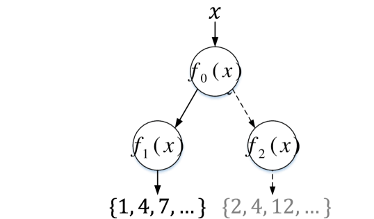
Figure 1: Left: Pseudocode for prediction where $f_{\mathrm{n}}(x)$ evaluates the node’s route, $\mbox{Predict}_{y}(x)$ evaluates a per-class regressor, $\widehat{\mathbf{recall}}(\circ)$ is an empirical bound on the recall of a node $(\circ)$ (see section 3.1), and $x\wedge\{(n:1)\}$ indicates the addition of a sparse feature with index $n$ and value $1$. Right: An example is routed through the tree to a leaf node associated with a set of eligible classes.

1.1 Prior Work

The LOMTree[7, 8] is the closest prior work. It misses on space requirements: up to a factor of 64 more space than OAA was used experimentally. Despite working with radically less space we show the Recall Tree typically provides better predictive performance. The key differences here are algorithmic: A tighter reduction at internal nodes and the one-against-some approach yields generally better performance despite much tighter resource constraints.

Boosting trees [13] for multiclass learning [24] on a generalized notion of entropy are known to results in low 0/1 loss. Relative to these works we show how to efficiently achieve weak learning by reduction to binary classification making this approach empirically practical. We also address a structural issue in the multiclass analysis (see section 3.3).

Other approaches such as hierarchical softmax (HSM) and the the Filter Tree [3] use a fixed tree structure [18]. In domains in which there is no prespecified tree hierarchy, using a random tree structure can lead to considerable underperformance as shown previously [1, 8].

Most other approaches in extreme classification either do not work online [17, 20] or only focus on speeding up either prediction time or training time but not both. Most of the works that enjoy sublinear inference time (but (super)linear training time) are based on tree decomposition approaches. In [17] the authors try to add tree structure learning to HSM via iteratively clustering the classes. While the end result is a classifier whose inference time scales logarithmically with the number of classes, the clustering steps are batch and scale poorly with the number of classes. Similar remarks apply to [1] where the authors propose to learn a tree by solving an eigenvalue problem after (OAA) training. The work of [27] is similar in spirit to ours, as the authors propose to learn a label filter to reduce the number of candidate classes in an OAA approach. However they learn the tree after training the underlying OAA predictors while here we learn and, more crucially, use the tree during training of the OAS predictors. Among the approaches that speed up training time we distinguish exact ones [9, 25] that have only been proposed for particular loss functions and approximate ones such as negative sampling as used e.g. in [26]. Though these techniques do not address inference time, separate procedures for speeding up inference (given a trained model) have been proposed [22]. However, such two step procedures can lead to substantially suboptimal results.

2 The Recall Tree Algorithm

Here we present a concrete description of the Recall Tree and defer all theoretical results that motivate our decisions to the next section. The Recall Tree maintains one predictor for each class and a tree whose purpose is to eliminate predictors from consideration. We refer to the per-class predictors as one-against-some (OAS) predictors. The tree creates a high recall set of candidate classes and then leverages the OAS predictors to achieve precision. Crucially, the leaves of the tree do not partition the set of classes: classes can (and do) have support at multiple leaves.

1 Algorithm:  Recall_Tree_Train

Input: Example $(x,y)$; Root node $n$

Result: Updated tree with root at $n$

2 do

3       $\mathbf{update\_router}(x,y,\mathrm{n})$ ;

4       $\mathrm{r}\leftarrow f_{\mathrm{n}}(x)>0$ ? n.left : n.right ;

5       $\mathbf{update\_candidates}(x,y,\mathrm{r})$ ;

6       if $\widehat{\mathbf{recall}}(\mathrm{n})>\widehat{\mathbf{recall}}(\mathrm{r})$ then

7             break

8       end if

9      $\mathrm{n}\leftarrow\mathrm{r}$;

10       $x\leftarrow x\cup\{(n:1)\}$

11while n.leaf is false;

12$\mathbf{update\_predictors}(x,y,\mathrm{n.candidates})$ ;

(a) An input labeled example descends the tree updating routers at the nodes until reaching a leaf or a recall estimate declines, leading to an early break. Here, $\mathbf{update\_candidates}$ updates the set of candidate labels at each node and $\mathbf{update\_predictors}$ updates the one-against-some predictors upon breaking; and $\widehat{\mathbf{recall}}(\circ)$ is a an empirical bound on the recall of a node $(\circ)$ (see section 3.1).

1 Algorithm:  update_router

Input: Example $(x,y)$; Node $n$

Result: Update node $n$

2 $\hat{H}_{\mathrm{left}},\hat{H}_{\mathrm{left}}^{\prime}\doteq\mathbf{entropy}(\mathrm{n.left},y)$ ;

3 $\hat{H}_{\mathrm{right}},\hat{H}_{\mathrm{right}}^{\prime}\doteq\mathbf{entropy}(\mathrm{n.right},y)$ ;

4 $\hat{H}_{\mathrm{|left}}\doteq\frac{\mathrm{n.left.total}}{\mathrm{n.total}}\hat{H}_{\mathrm{left}}^{\prime}+\frac{\mathrm{n.right.total}}{\mathrm{n.total}}\hat{H}_{\mathrm{right}}$ ;

5 $\hat{H}_{\mathrm{|right}}\doteq\frac{\mathrm{n.left.total}}{\mathrm{n.total}}\hat{H}_{\mathrm{left}}+\frac{\mathrm{n.right.total}}{\mathrm{n.total}}\hat{H}_{\mathrm{right}}^{\prime}$ ;

6 $\widehat{\Delta H}_{\mathrm{post}}\leftarrow\hat{H}_{\mathrm{|left}}-\hat{H}_{\mathrm{|right}}$ ;

$\mathrm{Learn}_{n}(x,|\widehat{\Delta H}_{\mathrm{post}}|,\mathrm{sign}(\widehat{\Delta H}_{\mathrm{post}}))$

(b) Here, $\mathbf{entropy}$ computes the empirical entropy of labels incident on a node without and with (respectively) an extra label $y$. $\hat{H}_{\mathrm{|left}}$ is an estimate of the average entropy if the example is routed left. $\mathrm{Learn}_{n}(x,w,y)$ is an importance-weighted update to the binary classifier $f(x)$ for node $n$ with features $x$, label $y$, and weight $w$.

Figure 2: Learning procedure.

Figure 2 outlines the learning procedures, which we now describe in more detail. Each node in the tree maintains a set of statistics. First, each node $n$ maintains a router, denoted $f_{\mathrm{n}}$, that maps an example to either a left or right child. This router is implemented as a binary classifier. Second, each node maintains a histogram of the labels of all training examples that have been routed to, or through, that node. This histogram is used in two ways: (1) the most frequent classes form the competitor set for the OAS predictors; (2) the histogram is used to decide whether the statistics at each node can be trusted. This is a crucial issue with trees because a child node sees fewer data than its parent. Therefore we do not simply rely on the empirical recall (i.e. the observed fraction of labels that fall into the most frequent $F$ labels at this node) of a node since such estimate can have considerable variance at deep nodes. Instead, we use a lower bound of the true recall which we compute via an empirical Bernstein inequality (see Section 3.1).

Learning the predictors for each class In Figure 2(a) $\mathbf{update\_predictors}$ updates the candidate set predictors using the standard OAA strategy restricted to the set of eligible classes. If the true label is not in the $F$ most frequent classes at this node then no update occurs.

Learning the set of candidates in each node In Figure 2(a) $\mathbf{update\_candidates}$ updates the count of the true label at this node. At each node, the most frequent $F$ labels are the candidate set.

Learning the routers at each node In Figure 2(b) $\mathbf{update\_router}$ updates the router at a node by optimizing the decrease in the entropy of the label distribution (the label entropy) due to routing. This is in accordance with our theory (Section 3.3). The label entropy for a node is estimated using the empirical counts of each class label entering the node. These counts are reliable as $\mathbf{update\_router}$ is only called for the root or nodes whose true recall bound is better than their children. The expected label entropy after routing is estimated by averaging the estimated label entropy of each child node, weighted by the fraction of examples routing left or right. Finally, we compute the advantage of routing left vs. right by taking the difference of the expected label entropies for routing left vs. right. The sign of this difference determines the binary label for updating the router.

Tree depth control We calculate a lower bound $\widehat{\mathbf{recall}}(\mathrm{n})$ on the true recall of node $n$ (Section 3.1), halting descent as in Figure 2(a). As we descend the tree, the bound first increases (empirical recall increases) then declines (variance increases). We also limit the maximum depth $d$ of the tree. This parameter is typically not operative but adds an additional safety check and sees some use on datasets where multipasses are employed.

3 Theoretical Motivation

Online construction of an optimal logarithmic time predictor for multiclass classification given an arbitrary fixed representation at each node appears deeply intractable. A primary difficulty is that decisions have to be hard since we cannot afford to maintain a distribution over all class labels. Choosing a classifier so as to minimize error rate has been considered for cryptographic primitives [5] so it is plausibly hard on averager rather than merely hard in the worst case. Furthermore, the joint optimization of all predictors does not nicely decompose into independent problems. Solving the above problems requires an implausible break-through in complexity theory which we do not achieve here. Instead, we use learning theory to assist the design by analyzing various simplifications of the problem.

3.1 One-Against-Some Prediction and Recall

For binary classification, branching programs [15] result in exponentially more succinct representations than decision trees [13] by joining nodes to create directed acyclic graphs. The key observation is that nodes in the same level with a similar distribution over class labels can be joined into one node, implying that the number of nodes at one level is only $\theta(1/\gamma)$ where $\gamma$ is the weak learning parameter rather than exponential in the depth. This approach generally fails in the multiclass setting because covering the simplex of multiclass label distributions requires $(K-1)^{\theta(1/\gamma)}$ nodes.

One easy special case exists. When the distribution over class labels is skewed so one label is the majority class, learning a minimum entropy classifier is equivalent to predicting whether the class is the majority or not. There are only $K$ possible OAS predictors of this sort so maintaining one for each class label is computationally tractable.

Using OAS classifiers creates a limited branching program structure over predictions. Aside from the space savings generated, this also implies that nodes deep in the tree use many more labeled examples than are otherwise available. In finite sample regimes, which are not covered by these boosting analyses, having more labeled samples implies a higher quality predictor as per standard sample complexity analysis.

A fundamental issue with a tree-structured prediction is that the number of labeled examples incident on the root is much larger than the number of labeled examples incident on a leaf. This potentially leads to: (1) underfitting toward the leaves; and (2) insufficient representation complexity toward the root. Optimizing recall, rather than accuracy, ameliorates this drawback. Instead of halting at a leaf, we can halt at an internal node $n$ for which the top $F$ most frequent labels contain the true answer with a sufficiently high probability. When $F=O(\log K)$ this does not compromise the goal of achieving logarithmic time classification.

Nevertheless, as data gets divided down the branches of the tree, empirical estimates for the “top $F$ most frequent labels” suffer from a substantial missing mass problem [11]. Thus, instead of computing empirical recall to determine when to halt descent, we use an empirical Bernstein (lower) bound [16], which is summarized by the following proposition.

Proposition 1.

For all learning problems $D$ and all nodes $n$ in a fixed tree there exists a constant $\lambda>0$ such that with probability $1-\delta$:

$$r_{n}\geq\hat{r}_{n}-\sqrt{\frac{\lambda\hat{r}_{n}(1-\hat{r}_{n})}{m_{n}}}-\frac{\lambda}{m_{n}}$$ (1)

where $\hat{r}_{n}$ is the empirical frequency amongst $m_{n}$ events that the true label is in the top $F$ labels and $r_{n}$ is the expected value in the population limit.

Reducing the depth of the tree by using a bound on $r_{n}$ and joining labeled examples from many leaves in a one-against-some approach both relieves data sparsity problems and allows greater error tolerance by the root node.

3.2 Path Features

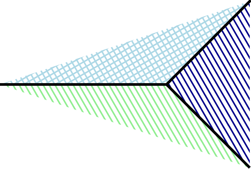
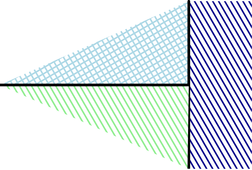
Figure 3: Two different distributions over class labels in the plane with each color/pattern representing support for a single class label. The left distribution is easily solved with an OAA classifier while the right distribution is easily solved with a decision tree.

The relative representational power of different solutions is an important consideration. Are OAA types of representations inherently more or less powerful than a tree based representation? Figure 3 shows two learning problems illustrating two extremes under the assumption of a linear representation.

Linear OAA: If all the class parameter vectors happen to have the same magnitude then OAA classification is equivalent to finding the nearest neighbor amongst a set of vectors (one per class) which partition the space into a Voronoi diagram as in 3 on the left. The general case, with unequal vectors corresponds to a weighted Voronoi diagram where the magnitude of two vectors sharing a border determines the edge of the partition. No weighted Voronoi diagram can account for the partition on the right.

Trees: If the partition of a space can be represented by a sequence of conditional splits, then a tree can represent the solution accurately as in 3 on the right. On the other hand, extra work is generally required to represent a Voronoi diagram as on the left. In general, the number of edges in a multidimensional Voronoi diagram may grow at least quadratically in the number of points implying that the number of nodes required for a tree to faithfully represent a Voronoi diagram is at least $\Theta(n^{2})$.

Based on this, neither tree-based nor OAA style prediction is inherently more powerful, with the best solution being problem dependent.

Since we are interested in starting with a tree-based approach and ending with a OAS classifier there is a simple representational trick which provides the best of both worlds. We can add features which record the path through the tree. To be precise, let $T$ be a tree and $\mbox{path}_{T}(x)$ be a vector with one dimension per node in $T$ which is set to $1$ if $x$ traverses the node and $0$ otherwise. The following proposition holds.

Proposition.

For any learning problem $D$ for which a tree $T$ achieves error rate $\epsilon$, $\mbox{OAA}(x,\mbox{path}_{T}(x))$ with a linear representation can achieve error rate $\epsilon$.

Linear representations are special, because they are tractably analyzed and because they are the fundamental building blocks around which many more complex representations are built. Hence, this representational change eases prediction in many common settings.

Proof.

A linear OAA classifier is defined by a matrix $w_{iy}$ where $i$ ranges over the input and $y$ ranges over the labels. Let $w_{iy}=0$ by default and $1$ when $i$ corresponds to a leaf for which the tree predicts $y$. Under this representation, the prediction of $\mbox{OAA}(x,\mbox{path}_{T}(x))$ is identical to $T(x)$, and hence achieves the same error rate. ∎

3.3 Optimization Objective

The Shannon Entropy of class labels is optimized in the router of figure 2(b). Why?

Since the Recall Tree jointly optimizes over many base learning algorithms, the systemic properties of the joint optimization are important to consider. A theory of decision tree learning as boosting [13] provides a way to understand these joint properties in a population limit (or equivalently on a training set iterated until convergence). In essence, the analysis shows that each level of the decision tree boosts the accuracy of the resulting tree with this conclusion holding for several common objectives.

In boosting for multiclass classification [7, 8, 24], it is important to achieve a weak dependence on the number of class labels. Shannon Entropy is particularly well-suited to this goal, because it has only a logarithmic dependence on the number of class labels. Let $\pi_{i|n}$ be the probability that the correct label is $i$, conditioned on the corresponding example reaching node $n$. Then $H_{n}=\sum_{i=1}^{K}\pi_{i|n}\log_{2}\frac{1}{\pi_{i|n}}$ is the Shannon entropy of class labels reaching node $n$.

For this section, we consider a simplified algorithm which neglects concerns of finite sample analysis, how optimization is done, and the leaf predictors. What’s left is the value of optimizing the router objective. We consider an algorithm which recursively splits the leaf with the largest fraction $f$ of all examples starting at the root and reaching the leaf. The leaf is split into two new leaves to the left $l$ and right $r$. If $f_{l}$ and $f_{r}$ are the fraction of examples going left and right, the split criterion minimizes the expectation over the leaves of the average class entropy, $f_{l}H_{l}+f_{r}H_{r}$. This might be achieved by $\mathbf{update\_router}$ in Figure 2(a) or by any other means. With this criterion we are in a position to directly optimize information boosting.

Definition 1.

($\gamma$-Weak Learning Assumption) For all distributions $n(x,y)$ a learning algorithm using examples $(x,y)^{*}$ IID from $n$ finds a binary classifier $c:X\rightarrow\{l,r\}$ satisfying

$$f_{l}H_{l}+f_{r}H_{r}\leq H_{n}-\gamma\,\,\,\,.$$

This approach is similar to previous [24] except that we boost in an additive rather than a multiplicative sense. This is good because it suppresses an implicit dependence on $K$ (since for any nontrivial $\gamma$ there exists a $K$ such that with a uniform distribution $U$, $H_{U}(1-\gamma)>1$), yeilding a strictly stronger result.

As long as Weak Learning occurs, we can prove the following theorem.

Theorem 2.

If $\gamma$ Weak Learning holds for every node in the tree and nodes with the largest fraction of examples are split first, then after $t>2$ splits the multiclass error rate $\epsilon$ of the tree is bounded by:

$$\epsilon\leq H_{1}-\gamma(1+\ln t)$$

where $H_{1}$ is the entropy of the marginal distribution of class labels.

The proof in appendix A reuses techniques from [8, 13] but has a tighter result.

The most important observation from the theorem is that as $t$ (the number of splits) increases, the error rate is increasingly bounded. This rate depends on $\ln t$ agreeing with the intuition that boosting happens level by level in the tree. The dependence on the initial entropy $H_{1}$ shows that skewed marginal class distributions are inherently easier to learn than uniform marginal class distributions, as might be expected. These results are similar to previous results [7, 8, 13, 24] with advantages. We handle multiclass rather than binary classification [13], we bound error rates instead of entropy [7, 8], and we use additive rather than multiplicative weak learning [24].

4 Empirical Results

We study several questions empirically.

1. What is the benefit of using one-against-some on a recall set?

2. What is the benefit of path features?

3. Is the online nature of the Recall Tree useful on nonstationary problems?

4. How does the Recall Tree compare to one-against-all statistically and computationally?

5. How does the Recall Tree compare to LOMTree statistically and computationally?

Throughout this section we conduct experiments using learning with a linear representation.

4.1 Datasets

Table 1: Datasets used for experimentation.

Dataset	Task	Classes	Examples
ALOI[10]	Visual Object Recognition	$1k$	$10^{5}$
Imagenet[19]	Visual Object Recognition	$\approx 20k$	$\approx 10^{7}$
LTCB[14]	Language Modeling	$\approx 80k$	$\approx 10^{8}$
ODP[2]	Document Classification	$\approx 100k$	$\approx 10^{6}$

Table 1 overviews the data sets used for experimentation. These include the largest datasets where published results are available for LOMTree (Aloi, Imagenet, ODP), plus an additional language modeling data set (LTCB). Implementations of the learning algorithms, and scripts to reproduce the data sets and experimental results, are available at (url redacted). Additional details about the datasets can be found in Appendix B.

4.2 Comparison with other Algorithms

In our first set of experiments, we compare Recall Tree with a strong computational baseline and a strong statistical baseline. The computational baseline is LOMTree, the only other online logarithmic-time multiclass algorithm we know of. The statistical baseline is OAA, whose statistical performance we want to match (or even exceed), and whose linear computational dependence on the number of classes we want to avoid. Details regarding the experimental methodology are in Appendix C. Results are summarized in Figure 4.

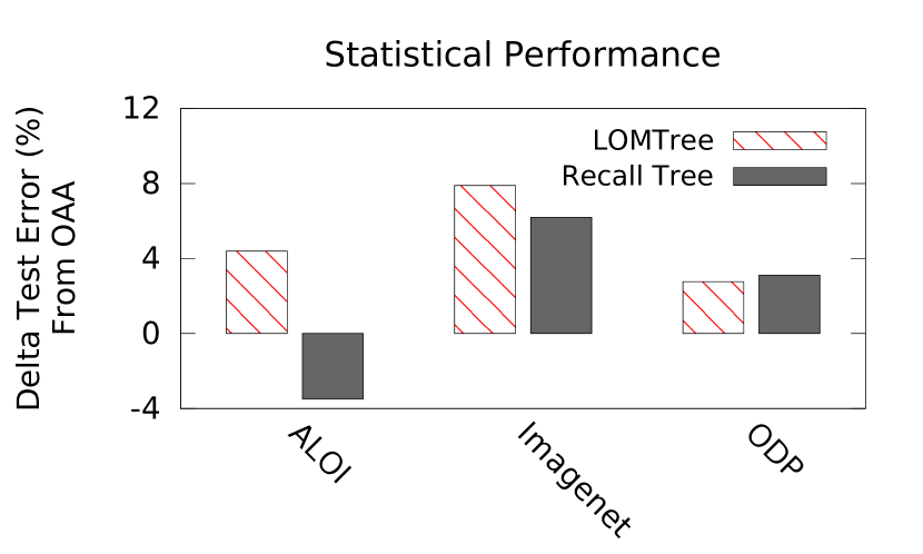
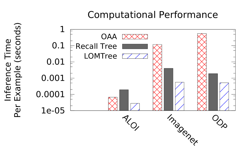
Figure 4: Empirical comparison of statistical (left) and computational (right) performance of Recall Tree against two strong competitors: OAA (statistically good) and LOMTree (computationally good). Recall Tree has $\mathrm{poly}(log)$ dependence upon number of classes (like LOMTree) but can surpass OAA statistically.

Comparison with LOMTree

The Recall Tree uses a factor of 32 less state than the LOMTree which makes a dramatic difference in feasibility for large scale applications. Given this state reduction, the default expectation is worse prediction performance by the Recall Tree. Instead, we observe superior or onpar statistical performance despite the state constraint. This typically comes with an additional computational cost since the Recall Tree evaluates a number of per-class predictors.

Comparison with OAA

On one dataset (Aloi) prediction performance is superior to OAA while on the others it is somewhat worse.

Computationally OAA has favorable constant factors since it is highly amenable to vectorization. Conversely, the conditional execution pattern of the Recall Tree frustrates vectorization even with example mini-batching. Thus on ALOI although Recall Tree does on average 50 hyperplane evaluations per example while OAA does 1000, OAA is actually faster: larger numbers of classes are required to experience the asymptotic benefits. For ODP with $\sim{}10^{5}$ classes, with negative gradient subsampling and using 24 cores in parallel, OAA is about the same wall clock time to train as Recall Tree on a single core. Negative gradient sampling does not improve inference times, which are roughly 300 times slower for OAA than Recall Tree on ODP.

4.3 Online Operation

In this experiment we leverage the online nature of the algorithm to exploit nonstationarity in the data to improve results. This is not something that is easily done with batch oriented algorithms, or with algorithms that post-process a trained predictor to accelerate inference.

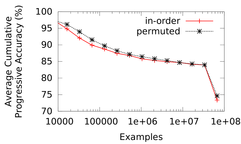
(a) When the LTCB dataset is presented in the original order, Recall Tree is able to exploit sequential correlations for improved performance. After all examples are processed, the average progressive accuracy is 73.3% vs. 74.6%.

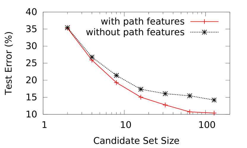
(b) Test error on ALOI for various candidate set sizes, with or without path features (all other parameters held fixed). Using multiple predictors per leaf and including path features improves performance.

Figure 5:

We consider two versions of LTCB. In both versions the task is to predict the next word given the previous 6 tokens. The difference is that in one version, the Wikipedia dump is processed in the original order (“in-order”); whereas in the other version the training data is permuted prior to input to the learning algorithm (“permuted”). We assess progressive validation loss [6] on the sequence. The result in Figure 5(a) confirms the Recall Tree is able to take advantage of the sequentially revealed data; in particular, the far-right difference in accuracies is significant at a factor $P<0.0001$ according to an $N-1$ Chi-squared test.

4.4 Path Features and Multiple Predictors

Two differences between Recall Tree and LOMTree are the use of multiple predictors at each tree node and the augmentation of the example with path features. In this experiment we explore the impact of these design choices using the ALOI dataset.

Figure 5(b) shows the effect of these two aspects on statistical performance. As the candidate set size is increased, test error decreases, but with diminishing returns. Disabling path features degrades performance, and the effect is more pronounced as the candidate set size increases. This is expected, as a larger candidate set size decreases the difficulty of obtaining good recall (i.e., a good tree) but increases the difficulty of obtaining good precision (i.e., good class predictors), and path features are only applicable to the latter. All differences here are significant at a $P<0.0001$ according to an $N-1$ Chi-squared test, except for when the candidate set size is $2$, where there is no significant difference.

4.5 The Empirical Bernstein Bound

Is the empirical Bernstein bound used helpful? To test this we trained on the LTCB dataset with a multiplier on the bound of either $0$ (i.e. just using empirical recall directly) or $1$. The results are stark: with a multiplier of $1$, the test error was $78\%$ while with a multiplier of $0$ the test error was $91\%$. Clearly, in the small samples per class regime this form of direct regularization is extraordinarily helpful.

5 Conclusion

In this work we proposed the Recall Tree, a reduction of multiclass to binary classification, which operates online and scales logarithmically with the number of classes. Unlike the LOMTree [8], we share classifiers among the nodes of the tree which alleviates data sparsity at deep levels while greatly reducing the required state. We also use a tighter analysis which is more closely followed in the implementation. These features allow us to reduce the statistical gap with OAA while still operating many orders of magnitude faster for large $K$ multiclass datasets. In the future we plan to investigate multiway splits in the tree since $O(\log K)$-way splits does not affect our $O(\textrm{poly}\log K)$ running time and they might reduce contention in the root and nodes high in the tree.

Acknowledgements We would like to thank an anonymous reviewer for NIPS who spotted an error in the theorem proof and made several good suggestions for improving it.

Appendix A Proof of theorem 2

Proof.

For the fixed tree at timestep $t$ (there have been $t-1$ previous splits) with a fixed partition function in the nodes, the weighted entropy of class labels is $W_{t}=\sum_{\{n\in\mbox{Leaves}\}}f_{n}H_{n}.$

When we split the $t$th node, the weak learning assumption implies entropy decreases by $\gamma$ according to:

$$H_{n}\geq\left(\frac{f_{l}}{f_{n}}H_{l}+\frac{f_{r}}{f_{n}}H_{r}\right)+\gamma$$

where $\gamma$ is the advantage of the weak learner. Hence,

$$W_{t}-W_{t+1}=f_{n}H_{n}-f_{l}H_{l}-f_{r}H_{r}\geq f_{n}\gamma\,\,\,\,.$$

We can bound $f_{n}$ according to

$$\max_{n}f_{n}\geq\frac{1}{t}$$

which implies

$$W_{t}-W_{t+1}\geq\frac{\gamma}{t}$$

. This can be solved recursively to get:

$$W_{t+1} \leq W_{1}-\gamma\sum_{i=1}^{t}\frac{1}{i}$$

$$\leq W_{1}-\gamma\left(1+\int_{i=1}^{t}\frac{1}{i}di\right)$$

$$=W_{1}-\gamma(1+\ln t)$$

$$=H_{1}-\gamma(1+\ln t)$$

where the second inequality follows from bounding each term of the sum with successive integrals, and $H_{1}$ is the marginal Shannon entropy of the class labels.

To finish the proof, we bound the multiclass loss in terms of the average entropy. For any leaf node $n$ we can assign the most likely label, $y=\arg\max_{i}\pi_{ni}$ so the error rate is $\epsilon_{n}=1-\pi_{ny}$.

$$W_{t+1} =\sum_{\{n\in\mbox{Leaves}\}}f_{n}\sum_{i}\pi_{ni}\ln\frac{1}{\pi_{ni}}$$

$$\geq\sum_{\{n\in\mbox{Leaves}\}}f_{n}\sum_{i}\pi_{ni}\ln\frac{1}{\pi_{ny}}$$

$$=\sum_{\{n\in\mbox{Leaves}\}}f_{n}\ln\frac{1}{1-\epsilon_{n}}$$

$$\geq\sum_{\{n\in\mbox{Leaves}\}}f_{n}\epsilon_{n}=$$

$$=\epsilon$$

Putting these inequalities together we have:

$$\epsilon\leq H_{1}-\gamma(1+\ln t)$$

∎

Appendix B Datasets

ALOI [10] is a color image collection of one-thousand small objects recorded for scientific purposes [10]. We use the same train-test split and representation as Choromanska et. al. [8].

Imagenet consists of features extracted from intermediate layers of a convolutional neural network trained on the ILVSRC2012 challenge dataset. This dataset was originally developed to study transfer learning in visual tasks [19]; more details are at http://www.di.ens.fr/willow/research/cnn/. We utilize a predictor linear in this representation.

LTCB is the Large Text Compression Benchmark, consisting of the first billion bytes of a particular Wikipedia dump [14]. Originally developed to study text compression, it is now commonly used as a language modeling benchmark where the task is to predict the next word in the sequence. We limit the vocabulary to 80000 words plus a single out-of-vocabulary indicator; utilize a model linear in the 6 previous unigrams, the previous bigram, and the previous trigram; and utilize a 90-10 train-test split on entire Wikipedia articles.

ODP[2] is a multiclass dataset derived from the Open Directory Project. We utilize the same train-test split and labels from [8]. Specifically there is a fixed train-test split of 2:1, the representation of a document is a bag of words, and the class label is the most specific category associated with each document.

Appendix C Experimental Methodology

Table 2: Empirical comparison summary. When OAA training is accelerated using parallelism and gradient subsampling, wall clock times are parenthesized. Training times are for defaults, i.e., without hyperparameter optimization. Asterisked LOMTree results are from [8].

Dataset	Method	Test Error		Training Time	Inference Time
		Default	Tuned		per example
ALOI	OAA	12.2%	12.1%	571s	67$\mu$s
	Recall Tree	11.4%	8.6%	1972s	194$\mu$s
	LOMTree	21.4%	$16.5\%^{*}$	112s	28$\mu$s
Imagenet	OAA	84.7%	82.2%	446d (20.4h)	118ms
	Recall Tree	91.1%	88.4%	71.4h	4ms
	LOMTree	96.7%	$90.1\%^{*}$	14.0h	0.56ms
LTCB	OAA	78.7%	76.8%	764d (19.1h)	3600$\mu$s
	Recall Tree	78.0%	77.6%	4.8h	76$\mu$s
	LOMTree	78.4%	-	4.3h	51$\mu$s
ODP	OAA	91.2%	90.6%	133d (1.3h)	560ms
	Recall Tree	96.2%	93.8%	1.5h	1.9ms
	LOMTree	95.4%	$93.5\%^{*}$	0.6h	0.52ms

Default Performance Methodology

Algorithm	Parameter	Default Value
Binary	Learning Rate	1
	Loss	logistic
Recall Tree	Max Depth	$\log_{2}(\mbox{\#classes})$
	Num Candidates	$4\log_{2}(\mbox{\#classes})$
	Depth Penalty ($\lambda$)	1

Table 3: Algorithm hyperparameters for various algorithms. “Binary” refers to hyperparameters inherited via reduction to binary classification.

Hyperparameter selection can be computationally burdensome for large data sets, which is relevant to any claims of decreased training times. Therefore we report results using the default values indicated in Table 3. For the larger data sets (Imagenet, ODP), we do a single pass over the training data; for the smaller data set (ALOI), we do multiple passes over the training data, monitoring a 10% held-out portion of the training data to determine when to stop optimizing.

Tuned Performance Methodology

For tuned performance, we use random search over hyperparameters, taking the best result over 59 probes. For the smaller data set (ALOI), we optimize validation error on a 10% held-out subset of the training data. For the larger data sets (Imagenet, ODP), we optimize progressive validation loss on the initial 10% of the training data. After determining hyperparameters we retrain with the entire training set and report the resulting test error.

When available we report published LOMtree results, although they utilized a different method for optimizing hyperparameters.

Timing Measurements

All timings are taken from the same 24 core xeon server machine. Furthermore, all algorithms are implemented in the Vowpal Wabbit toolkit and therefore share file formats, parser, and binary classification base learner implying differences are attributable to the different reductions. Our baseline OAA implementation is mature and highly tuned: it always exploits vectorization, and furthermore can optionally utilize multicore training and negative gradient subsampling to accelerate training. For the larger datasets these latter features were necessary to complete the experiments: estimated unaccelerated training times are given, along with wall clock times in parenthesis.

References

- [1] Samy Bengio, Jason Weston, and David Grangier. Label embedding trees for large multi-class tasks. In Advances in Neural Information Processing Systems, pages 163–171, 2010.
- [2] Paul N Bennett and Nam Nguyen. Refined experts: improving classification in large taxonomies. In Proceedings of the 32nd international ACM SIGIR conference on Research and development in information retrieval, pages 11–18. ACM, 2009.
- [3] Alina Beygelzimer, John Langford, and Pradeep Ravikumar. Error-correcting tournaments. In Algorithmic Learning Theory, 20th International Conference, ALT 2009, Porto, Portugal, October 3-5, 2009. Proceedings, pages 247–262, 2009.
- [4] Kush Bhatia, Himanshu Jain, Purushottam Kar, Manik Varma, and Prateek Jain. Sparse local embeddings for extreme multi-label classification. In Advances in Neural Information Processing Systems, pages 730–738, 2015.
- [5] Avrim Blum, Merrick Furst, Michael Kearns, and Richard J Lipton. Cryptographic primitives based on hard learning problems. In Advances in cryptology—CRYPTO’93, pages 278–291. Springer, 1993.
- [6] Avrim Blum, Adam Kalai, and John Langford. Beating the hold-out: Bounds for k-fold and progressive cross-validation. In Proceedings of the Twelfth Annual Conference on Computational Learning Theory, COLT 1999, Santa Cruz, CA, USA, July 7-9, 1999, pages 203–208, 1999.
- [7] Anna Choromanska, Krzysztof Choromanski, and Mariusz Bojarski. On the boosting ability of top-down decision tree learning algorithm for multiclass classification. CoRR, abs/1605.05223, 2016.
- [8] Anna E Choromanska and John Langford. Logarithmic time online multiclass prediction. In Advances in Neural Information Processing Systems, pages 55–63, 2015.
- [9] Alexandre de Brébisson and Pascal Vincent. An exploration of softmax alternatives belonging to the spherical loss family. arXiv preprint arXiv:1511.05042, 2015.
- [10] Jan-Mark Geusebroek, Gertjan J Burghouts, and Arnold WM Smeulders. The Amsterdam library of object images. International Journal of Computer Vision, 61(1):103–112, 2005.
- [11] I. J. Good. The population frequencies of species and the estimation of population parameters. Biometrika, 40(16):237–264, 1953.
- [12] Kaiming He, Xiangyu Zhang, Shaoqing Ren, and Jian Sun. Deep residual learning for image recognition. CoRR, abs/1512.03385, 2015.
- [13] Michael Kearns and Yishay Mansour. On the boosting ability of top-down decision tree learning algorithms. In Proceedings of STOC, pages 459–468. ACM, 1996.
- [14] Matt Mahoney. Large text compression benchmark. http://www.mattmahoney.net/text/text.html, 2009.
- [15] Yishay Mansour and David McAllester. Boosting using branching programs. Journal of Computer and System Sciences, 64(1):103–112, 2002.
- [16] Andreas Maurer and Massimiliano Pontil. Empirical bernstein bounds and sample variance penalization. arXiv preprint arXiv:0907.3740, 2009.
- [17] Andriy Mnih and Geoffrey E Hinton. A scalable hierarchical distributed language model. In Advances in neural information processing systems, pages 1081–1088, 2009.
- [18] Frederic Morin and Yoshua Bengio. Hierarchical probabilistic neural network language model. In Proceedings of the international workshop on artificial intelligence and statistics, pages 246–252, 2005.
- [19] M. Oquab, L. Bottou, I. Laptev, and J. Sivic. Learning and transferring mid-level image representations using convolutional neural networks. In CVPR, 2014.
- [20] Yashoteja Prabhu and Manik Varma. Fastxml: A fast, accurate and stable tree-classifier for extreme multi-label learning. In Proceedings of the 20th ACM SIGKDD, pages 263–272. ACM, 2014.
- [21] Ryan Rifkin and Aldebaro Klautau. In defense of one-vs-all classification. The Journal of Machine Learning Research, 5:101–141, 2004.
- [22] Anshumali Shrivastava and Ping Li. Asymmetric lsh (alsh) for sublinear time maximum inner product search (mips). In Advances in Neural Information Processing Systems, pages 2321–2329, 2014.
- [23] Karen Simonyan and Andrew Zisserman. Very deep convolutional networks for large-scale image recognition. CoRR, abs/1409.1556, 2014.
- [24] Eiji Takimoto and Akira Maruoka. Top-down decision tree learning as information based boosting. Theor. Comput. Sci., 292(2):447–464, 2003.
- [25] Pascal Vincent, Alexandre de Brébisson, and Xavier Bouthillier. Efficient exact gradient update for training deep networks with very large sparse targets. In NIPS 28, pages 1108–1116, 2015.
- [26] Jason Weston, Samy Bengio, and Nicolas Usunier. WSABIE: scaling up to large vocabulary image annotation. In IJCAI 2011, Proceedings of the 22nd International Joint Conference on Artificial Intelligence, Barcelona, Catalonia, Spain, July 16-22, 2011, pages 2764–2770, 2011.
- [27] Jason Weston, Ameesh Makadia, and Hector Yee. Label partitioning for sublinear ranking. In Proceedings of the 30th International Conference on Machine Learning (ICML-13), pages 181–189, 2013.