Lepton flavor-violating decays of the Higgs boson
from sgoldstino mixing

Abstract

We study lepton flavor violation in a class of supersymmetric models with light sgoldstino – scalar superpartner of Goldstone fermions responsible for spontaneous supersymmetry breaking. Sgoldstino couplings to the Standard Model (SM) fermions are determined by the MSSM soft terms and, in general, provide with flavor violation in this sector. Sgoldstino admixture to the lightest Higgs boson results in changes of its coupling constants and, in particular, leads to lepton flavor-violating decay $h\to\tau\mu$ of the Higgs resonance. We discuss viability and phenomenological consequences of this scenario.

1 Introduction

Study of the Higgs boson properties is one of the priority problems since its discovery Aad:2012tfa ; Chatrchyan:2012xdj . Special attention is paid to flavor changing processes involving the Higgs boson and, in particular, to the lepton flavor-violating (LFV) Higgs boson decays Khachatryan:2015kon ; Aad:2015gha . Prospects of studying the LFV Higgs boson decays at the LHC experiments were discussed in Blankenburg:2012ex ; Harnik:2012pb ; Kopp:2014rva ; DiazCruz:2008ry ; Pilaftsis:1992st . In particular, it has been found that given strong constraints from FCNC physics sufficiently large branching ratios of the Higgs boson decays $h\to e\tau$ and $h\to\mu\tau$ are still allowed. Recently, the latter $h\to\mu\tau$ decay has drawn much attention because the latest results for upper limits on the branching ratio of $h\to\tau\mu$ decay have been reported by the ATLAS, ${\rm Br}(h\to\tau\mu)<1.85\times 10^{-2}$, and CMS, ${\rm Br}(h\to\tau\mu)<1.51\times 10^{-2}$ at 95% CL. At the same time, the CMS analysis revealed a small excess in this process with a significance of 2.4$\sigma$ which can be interpreted as LFV Higgs decay with branching ${\rm Br}(h\to\tau\mu)=8.4^{+3.9}_{-3.7}\times 10^{-3}$. Although not yet statistically significant, this excess is very intriguing. If confirmed, it would give direct indication on non-SM properties of the Higgs boson.

To explain this excess, various models of new physics have been studied, including Dery:2014kxa ; Campos:2014zaa ; Sierra:2014nqa ; Heeck:2014qea ; Crivellin:2015mga ; Dorsner:2015mja ; He:2015rqa ; Altmannshofer:2015esa ; Arganda:2015naa ; Botella:2015hoa ; Baek:2015mea ; Buschmann:2016uzg . In what follows, we will be interested in supersymmetric scenarios. LFV decays of the Higgs boson in MSSM was discussed in Brignole:2003iv ; Brignole:2004ah and recently in Arana-Catania:2013xma . Previous studies of $h\to\mu\tau$ decay with account of the CMS excess can be found in Refs. Arganda:2015uca , Aloni:2015wvn . These studies revealed that for a generic set of parameters predictions for ${\rm Br}(h\to\mu\tau)$ are very small for this decay to be observed at the LHC and only limited parameter space of MSSM is capable of explaining the CMS excess.

In this paper, we will be interested in explanation of the CMS excess within the framework of a particular class of supersymmetric models with low scale supersymmetry breaking (see, e.g Brignole:2003cm and recent studies in Petersson:2011in ; Antoniadis:2012ck ; Dudas:2012fa ; Dudas:2013mia ; Das:2015zwa . In these models, it is assumed that the scale of supersymmetry breaking $\sqrt{F}$ is not very far from the electroweak energy scale. In this case, particles responsible for the spontaneous supersymmetry breaking may show up already in the LHC experiments Shirai:2009kn ; Klasen:2006kb ; Brignole:1998me ; Petersson:2012dp ; Gorbunov:2000ht ; Gorbunov:2002er ; Demidov:2004qt ; Petersson:2015rza . This additional sector contains goldstino and its superpartners – sgoldstinos, which in the simplest case are scalars. The coupling constants of this sector to the SM particles are governed by the soft supersymmetry breaking parameters of supersymmetric model which are generally flavor violating and can lead to FCNC processes Gorbunov:2000th ; Brignole:2000wd ; Gorbunov:2000cz ; Gorbunov:2005nu ; Demidov:2006pt ; Demidov:2011rd ; Astapov:2015otc . The main idea for the explanation of the CMS excess is that the Higgs boson can mix with the scalar sgoldstino Bellazzini:2012mh ; Astapov:2014mea , while the latter has flavor-violating interactions with the SM fermions.

Below we calculate the contribution of the sgoldstino-Higgs mixing to $h\to\tau\mu$ decay and analyze constraints from relevant FCNC processes and from LHC data. We find that this mixing is capable of explaining the CMS excess in a part of the parameter space. Also we discuss possible implications of this scenario for the Higgs boson physics as well as for several FCNC processes. In Section 2 we describe the theoretical framework of low scale supersymmetry breaking models and discuss sgoldstino-Higgs mixing. In Section 3 we turn to the phenomenological analysis, performing a scan over relevant parameter space of the model and discussing experimental constraints. In Section 4 we present the results of the scan and reveal interesting features which can be useful to verifying this scenario. Section 5 contains our conclusions and several technical aspects are left for appendices.

2 Theoretical framework

Here we briefly describe the main features of the supersymmetric model with light sgoldstinos. In addition to the SM fields and their superpartners of the conventional MSSM we introduce goldstino chiral superfield $\Phi=\phi+\sqrt{2}\theta\widetilde{G}+F_{\phi}\theta^{2}$. Here $\tilde{G}$ is the Goldstone fermion, $\phi$ is the sgoldstino field and $F_{\phi}$ is the auxiliary field. Due to some dynamics in the hidden sector, the field $F_{\phi}$ acquires vacuum expectation value which breaks SUSY spontaneously. We restrict ourselves to the simplest set of operators which reproduces soft SUSY-breaking parameters of MSSM after spontaneous supersymmetry breaking Petersson:2011in ; Gorbunov:2001pd . We use the following lagrangian

$$\mathcal{L}_{\text{model}}=\mathcal{L}_{\text{K{\"{a}}hler}}+\mathcal{L}_{\text{superpotential}}.$$ (2.1)

The contribution to the Kähler potential has the form

$$\mathcal{L}_{\text{K{\"{a}}hler}}=\int\,d^{2}\theta\,d^{2}\macc@depth\char 1\relax\frozen@everymath{\macc@group}\macc@set@skewchar\macc@nested@a 111{}\,\sum_{k}\left(1-\frac{m_{k}^{2}}{F^{2}}\Phi^{\dagger}\Phi\right)\Phi^{\dagger}_{k}e^{g_{1}V_{1}+g_{2}V_{2}+g_{3}V_{3}}\Phi_{k},$$ (2.2)

where the sum goes over all chiral MSSM superfields and we implicitly assume possibility of nontrivial flavor structure for the soft parameters $m_{k}^{2}$ of sleptons and squarks. The contribution from the superpotential is

$$\begin{aligned} \mathcal{L}_{\text{superpotential}}=&\int\,d^{2}\theta\,\Biggl{\{}\epsilon_{ij}\Biggl{(}\left(\mu-\frac{B}{F}\Phi\right)H_{d}^{i}H_{u}^{j}+\left(Y_{ab}^{L}+\frac{A_{ab}^{L}}{F}\Phi\right)L_{a}^{j}E_{b}^{c}H_{d}^{i}+\\ &+\left(Y_{ab}^{D}+\frac{A_{ab}^{D}}{F}\Phi\right)Q_{a}^{j}D_{b}^{c}H_{d}^{i}+\left(Y_{ab}^{U}+\frac{A_{ab}^{U}}{F}\Phi\right)Q_{a}^{i}U_{b}^{c}H_{d}^{j}\Biggr{)}+\\ &+\frac{1}{4}\sum_{\alpha}\left(1+\frac{2M_{\alpha}}{F}\Phi\right)\text{Tr}\,W^{\alpha}W^{\alpha}\Biggr{\}}+\text{h.c.}\end{aligned}$$ (2.3)

Here $B$, $A_{ab}^{L,D,U}$ and $M_{\alpha}$, $a,b,\alpha=1,2,3$ are the soft MSSM parameters. For lagrangian of the hidden sector, we choose the following form

$$\mathcal{L}_{\Phi}=\int\,d^{2}\theta\,d^{2}\macc@depth\char 1\relax\frozen@everymath{\macc@group}\macc@set@skewchar\macc@nested@a 111{}\left(\Phi^{\dagger}\Phi+\widetilde{K}(\Phi^{\dagger},\Phi)\right)-\left(\int d^{2}\theta F\Phi+\text{h.c.}\right),$$ (2.4)

where the first term is the canonical kinetic term while the second one, $\widetilde{K}(\Phi^{\dagger},\Phi)$, represents some complicated dynamics in the hidden sector and is suppressed by powers of $F$. The last linear term in the superpotential of Eq. (2.4) forces the auxiliary field $F_{\phi}$ to acquire non-zero vacuum expectation value $\langle F_{\phi}\rangle=F+\mathcal{O}\left(\frac{1}{F}\right)$ and hence triggers spontaneous supersymmetry breaking. In what follows, we assume that all the parameters of the lagrangian (2.1) – (2.4) are real and hence ignore possible CP-violation  After integrating out the auxiliary fields of sgoldstino and Higgs chiral superfields as well as auxiliary fields of vector superfields containing the SM gauge bosons and assuming that $\sqrt{F}$ is the largest energy scale of the model, the potential of the Higgs sector can be written as an expansion in powers of $1/F$ as follows

$$V_{\text{model}}=V_{\text{MSSM}}+V^{(1)}+V^{(2)}+...\;,$$ (2.5)

where $V_{\text{MSSM}}$ is the MSSM scalar potential Martin:1997ns

$$\begin{aligned} V_{\text{MSSM}}=&\left(|\mu|^{2}+m_{H_{u}}^{2}\right)\left(|H_{u}^{0}|^{2}+|H_{u}^{+}|^{2}\right)+\left(|\mu|^{2}+m_{H_{d}}^{2}\right)\left(|H_{d}^{0}|^{2}+|H_{d}^{+}|^{2}\right)+\\ &+\left(B\left(H_{u}^{+}H_{d}^{-}-H_{u}^{0}H_{d}^{0}\right)+\text{c.c.}\right)+\\ &+\frac{g_{1}^{2}+g_{2}^{2}}{8}\left(|H_{u}^{0}|^{2}+|H_{u}^{+}|^{2}-|H_{d}^{0}|^{2}-|H_{d}^{+}|^{2}\right)^{2}+\frac{g_{1}^{2}}{2}\left|H_{u}^{+}H_{d}^{0*}+H_{u}^{0}H_{d}^{-*}\right|^{2}.\end{aligned}$$ (2.6)

$V^{(1)}$ contains part of the potential responsible for Higgs-sgoldstino mixing

$$\begin{aligned} V_{\text{mixing}}=&\frac{\phi}{F}\Bigl{(}\mu\,\left(m_{H_{u}}^{2}+m_{H_{d}}^{2}\right)\left(H_{u}^{0}H_{d}^{0}\right)^{*}-\frac{g_{1}^{2}M_{1}+g_{2}^{2}M_{2}}{8}\left(|H_{u}^{0}|^{2}-|H_{d}^{0}|^{2}\right)^{2}-\\ &-B\mu\left(|H_{u}^{0}|^{2}+|H_{d}^{0}|^{2}\right)\Bigr{)}+\text{h.c.}\end{aligned}$$ (2.7)

The part $V^{(2)}$ contains, in particular, $1/F^{2}$ corrections to the MSSM Higgs potential

$$V^{(2)}=\frac{1}{F^{2}}\left|m_{H_{u}}^{2}H_{u}^{\dagger}H_{u}+m_{H_{d}}^{2}H_{d}^{\dagger}H_{d}-B\epsilon_{ij}H_{u}^{i}H_{d}^{j}\right|^{2}+...$$ (2.8)

Other contributions to the scalar potential in Eqs. (2.5) and (2.8) include sgoldstino potential, contributions of higher orders in $1/F$ and nonlinear interactions with sgoldstino which are not relevant for the present analysis.

Next, we expand Higgs $H_{u,d}^{0}$ and sgoldstino $\phi$ fields around their minima as follows

$$\begin{aligned} &H_{u}^{0}=v_{u}+\frac{1}{\sqrt{2}}\left(h\,\cos\alpha+H\,\sin\alpha\right)+\frac{\dot{\imath}}{\sqrt{2}}A\,\cos\beta,\\ &H_{d}^{0}=v_{d}+\frac{1}{\sqrt{2}}\left(-h\,\sin\alpha+H\,\cos\alpha\right)+\frac{\dot{\imath}}{\sqrt{2}}A\,\sin\beta,\\ &\phi=\frac{1}{\sqrt{2}}\left(s+\dot{\imath}p\right),\end{aligned}$$ (2.9)

where $v_{u,d}=\langle H_{u,d}^{0}\rangle$ and $v\equiv\sqrt{v_{u}^{2}+v_{d}^{2}}=174\leavevmode\nobreak\ \rm{GeV}$, $\tan\beta=\frac{v_{u}}{v_{d}}$. Mixing angle between gauge $({\rm Re}H_{u}^{0},\,{\rm Re}H_{d}^{0})$ and mass eigenstates $(h,\,H)$ is denoted by $\alpha$. By convention, $h$ is assumed to be lighter than $H$. $A$ is CP-odd neutral Higgs field, while $s$ and $p$ are scalar and pseudoscalar sgoldstino components. In what follows, we will work in the decoupling limit, i.e. $m_{A}\gg m_{h}$, or, equivalently $\cos\,\alpha\approx\sin\,\beta$, $\sin\,\alpha\approx-\cos\,\beta$. Substituting (2.9) into (2.7) and holding only quadratic terms, one gets the following mass matrix in scalar sector

$$\mathcal{M}_{s}^{2}=\left(\begin{matrix}m_{H}^{2}&0&\frac{Y}{F}\\ 0&m_{h}^{2}&\frac{X}{F}\\ \frac{Y}{F}&\frac{X}{F}&m_{s}^{2}\end{matrix}\right),$$ (2.10)

where the off-diagonal terms are

$$\begin{aligned} &X=2\mu^{3}\,v\,\sin\,2\beta+\frac{v^{3}}{2}(g_{1}^{2}\,M_{1}+g_{2}^{2}\,M_{2})\cos^{2}\,2\beta,\\ &Y=\mu\,v\,(m_{A}^{2}-2\mu^{2})+\frac{v^{3}}{4}\left(g_{1}^{2}M_{1}+g_{2}^{2}M_{2}\right)\,\sin 4\beta.\end{aligned}$$ (2.11)

In writing (2.9), we assume following Ref. Astapov:2014mea that sgoldstino field $\phi$ does not acquire non-zero vacuum expectation value. In this study, we address sufficiently small sgoldstino masses, hence the heavier Higgs boson $H$ decouples and the remaining light states can be approximated by the following linear combination

$$\left(\begin{matrix}\tilde{h}\\ \tilde{s}\end{matrix}\right)=\left(\begin{matrix}\cos\,\theta&-\sin\,\theta\\ \sin\,\theta&\cos\,\theta\end{matrix}\right)\left(\begin{matrix}h\\ s\end{matrix}\right).$$ (2.12)

The mixing angle can be obtained from the following equation

$$\tan 2\theta=\frac{2X}{F(m_{s}^{2}-m_{h}^{2})}.$$ (2.13)

In the decoupling regime, the $m_{h}^{2}$ parameter is given by

$$m_{h}^{2}=m_{Z}^{2}\cos^{2}{2\beta}+\frac{v^{2}}{F^{2}}\left(B\sin{2\beta}-2\mu^{2}\right)^{2}+{\rm loop}\;{\rm corrections}.$$ (2.14)

Let us note, that the second term in (2.14) coming from Eq. (2.8) at some values of parameters gives considerable contribution Petersson:2012nv and allows to reduce the level of fine-tuning as compared to the standard MSSM setup for $\sqrt{F}\sim$ few TeV, see Antoniadis:2014eta for details.

The mixing between the Higgs boson and sgoldstino results in modification of their coupling constants with the vector bosons and SM fermions. It is important for our study, that sgoldstino interactions with leptons are given by the soft trilinear couplings $A^{L}_{ab}$. In a generic model, their flavor structure is different from that of lepton Yukawa coupling constants. In this way, small admixture of sgoldstino to the lightest Higgs boson generates flavor violating couplings of the latter. To describe changes of the couplings, let us consider the relevant part of the lagrangian after the EWSB

$$\begin{aligned} &\mathcal{L}\supset Y^{L}_{ab}\,\macc@depth\char 1\relax\frozen@everymath{\macc@group}\macc@set@skewchar\macc@nested@a 111{e}_{b}\,l_{a}\left(1+\frac{h}{\sqrt{2}v}\right)+\frac{A^{L}_{ab}}{\sqrt{2}F}\macc@depth\char 1\relax\frozen@everymath{\macc@group}\macc@set@skewchar\macc@nested@a 111{e}_{b}\,l_{a}\,v_{d}\,s+\text{h.c.}\supset\\ &\supset(v_{d}\,\macc@depth\char 1\relax\frozen@everymath{\macc@group}\macc@set@skewchar\macc@nested@a 111{l}\,Y^{L}\,l_{L}+\text{h.c.})+\left(v_{d}\,\macc@depth\char 1\relax\frozen@everymath{\macc@group}\macc@set@skewchar\macc@nested@a 111{l}\left(\frac{Y^{L}}{\sqrt{2}v}\cos\theta-\frac{(A^{L})^{T}}{\sqrt{2}F}\sin\theta\right)l_{L}\tilde{h}+\text{h.c.}\right).\end{aligned}$$ (2.15)

Assuming the leptons to be in the mass basis $l=\left(e,\mu,\tau\right)^{\rm T}$ with $v_{d}Y_{ab}^{L}=-m_{a}\delta_{ab}$, we obtain

$$\mathcal{L}\supset-m_{a}\,\macc@depth\char 1\relax\frozen@everymath{\macc@group}\macc@set@skewchar\macc@nested@a 111{l}\,l^{a}-\tilde{h}\left(\macc@depth\char 1\relax\frozen@everymath{\macc@group}\macc@set@skewchar\macc@nested@a 111{l}\,l_{R}^{b}\,Y^{\tilde{h}}_{ab}+\text{h.c.}\right),$$ (2.16)

where the modified Yukawa couplings look as

$$Y^{\tilde{h}}_{ab}=\frac{m_{a}\,\delta_{ab}\,\cos\theta}{\sqrt{2}v}+\frac{v_{d}A^{L}_{ab}\,\sin\theta}{\sqrt{2}F}.$$ (2.17)

We see that $Y^{\tilde{h}}_{ab}\neq 0$ if $a\neq b$ and hence the LVF decays of the Higgs boson arise already at tree level. The decay width for $\tilde{h}\rightarrow l_{a}\,l_{b}$ with $a\neq b$ is given by Khachatryan:2015kon ; Harnik:2012pb

$$\Gamma(\tilde{h}\rightarrow l_{a}\,l_{b})=\Gamma(\tilde{h}\rightarrow\macc@depth\char 1\relax\frozen@everymath{\macc@group}\macc@set@skewchar\macc@nested@a 111{l}_{b}\,l_{a})+\Gamma(\tilde{h}\rightarrow\macc@depth\char 1\relax\frozen@everymath{\macc@group}\macc@set@skewchar\macc@nested@a 111{l}_{a}\,l_{b})=\frac{m_{\tilde{h}}}{8\pi}\left(|Y^{\tilde{h}}_{ab}|^{2}+|Y^{\tilde{h}}_{ba}|^{2}\right).$$ (2.18)

3 Analysis of the scenario

In this section, we describe the strategy which is used here to analyze phenomenological consequences of the scenario with lepton flavor-violating couplings of the Higgs resonance which appear from its interactions with the sector responsible for supersymmetry breaking. Although this scenario is quite general and allows for flavor violation in both quark and lepton sectors, in the following discussion we focus mainly on $\mu$–$\tau$ part in view of the CMS excess. We perform a scan over relevant part of the parameter space presented in Table 1.

$\tan\,\beta$	1.5 …50.5
$|\mu|$	$100$ …$2000$ GeV
$M_{1}$	100 $\ldots 2000\,\text{GeV}$
$M_{2}$	200 $\ldots 2000\,\text{GeV}$
$M_{3}$	1.5 $\ldots 4.0\,\text{TeV}$
$A_{\tau\tau},A_{\mu\tau},A_{\tau\mu}$	0.1 $\sqrt{F}$ $\ldots$ $\sqrt{F}$
$A_{\mu\mu}$	0.1 $\sqrt{F}$ $\ldots$ $0.5\sqrt{F}$
$m_{\text{sl}}$	4000 GeV $\ldots\sqrt{F}\,$

Table 1: Parameter space used in the analysis

We remind that the consistency of the effective field theory approach to the model (2.2)–(2.4) requires that the parameters which become soft terms after the spontaneous supersymmetry breaking should be smaller than $\sqrt{F}$. In what follows, we fix value of supersymmetry breaking scale to 8 TeV. We will comment on this choice later on. Note that we allow for rather large values of off-diagonal trilinear soft parameters $A_{\mu\mu},A_{\tau\tau},A_{\mu\tau}$ and $A_{\tau\mu}$ and following purely phenomenological approach assume no other sources of lepton flavor violation in the model. All soft masses of sleptons are chosen to be equal and we scan over their common value $m_{\text{sl}}$. While scanning over the soft parameters of the lepton sector, we take into account experimental constraint on slepton masses. Namely, we will require that the mass of the lightest slepton should be larger than $325\,\text{GeV}$ Aad:2014vma . In our analysis, we calculate spectrum of the lepton mass matrix and check whether this constraint on the smallest eigenvalue is fulfilled. The squark sector of the model is not considered here, and thus we independently scan over the mass parameter $m_{h}$ of the lightest Higgs boson entering the scalar mass matrix over the following interval $115$–$130$ GeV. We find that for the most interesting cases the mass parameter of the scalar sgoldstino should not be very heavy or very small. In the case of heavy sgoldstino, the mixing angle (2.13) is small and, as a consequence, the width of $\tilde{h}\to\mu\tau$ decay is suppressed. On the other hand, very light sgoldstinos with large Higgs boson admixture are phenomenologically unacceptable due to results from the LEP Schael:2006cr and Tevatron Abazov:2013gmz experiments. In what follows, we limit ourselves to the regimes in which the scalar sgoldstino mass parameter is somewhat smaller (90–114 GeV) or larger (150–200 GeV) than the Higgs boson mass. Some parameters, which are not of primary importance for the analysis, were fixed to reasonable benchmark values. In particular, we set the soft trilinear constant of b-quark $A_{bb}=0.5\,\sqrt{F}$ and the mass of pseudoscalar sgoldstino $m_{p}=200\,\text{GeV}$. For each chosen point in the parameter space, we find physical masses of the Higgs-like $m_{\tilde{h}}$ and sgoldstino-like states $m_{\tilde{s}}$, selecting models with the Higgs resonance lying in the mass range $m_{\tilde{h}}=125.09^{+0.24}_{-0.24}\leavevmode\nobreak\ \rm{GeV}$, calculate relevant observables which will be discussed below and find phenomenologically acceptable models.

Mixing of scalar sgoldstino with the lightest Higgs boson results in modifications of the Higgs signal strengths

$$\mu_{f}=\frac{\sigma(pp\rightarrow\tilde{h})\times{\rm Br}(\tilde{h}\rightarrow f)}{\sigma(pp\rightarrow h^{SM})\times{\rm Br}(h^{SM}\rightarrow f)},$$ (3.1)

where index $f$ stands for the following final states, $W^{+}\,W^{-}$, $ZZ$, $\gamma\,\gamma$, $\macc@depth\char 1\relax\frozen@everymath{\macc@group}\macc@set@skewchar\macc@nested@a 111{b}\,b$, $\tau^{+}\,\tau^{-}$ and $\mu^{+}\mu^{-}$. We calculate them using modified Higgs boson couplings presented in Appendix A. Sizable QCD corrections have been taken into account using general expressions from Ref. Spira:1997dg . For the diboson final states, the Higgs boson is mainly produced at the LHC via gluon-gluon fusion (ggh) channel and neglecting other production mechanisms is a fairly good approximation. In this case, one obtains

$$\frac{\sigma(pp\rightarrow\tilde{h})}{\sigma(pp\rightarrow h)_{\text{SM}}}\simeq\frac{\Gamma(\tilde{h}\rightarrow gg)}{\Gamma(h\rightarrow gg)_{SM}}=\frac{\left|\sum_{Q}A_{1/2}(\tau_{Q})\,\cos\theta+\frac{6M_{3}\pi v}{\alpha_{s}\,F}\,\sin\theta\right|^{2}}{\left|\sum_{Q}A_{1/2}(\tau_{Q})\right|^{2}}\;,$$ (3.2)

where the sum goes over all quarks; see Appendix A. It should be noticed, that both terms in the numerator, $\sum_{Q}A_{1/2}(\tau_{Q})$ and $\frac{6M_{3}\pi v}{\alpha_{s}\,F}$, can be of the same size. So, in the case when $M_{3}$ and $\sin\theta$ have different signs (for example in case of the negative value of the parameter $\mu$ and positive $M_{3}$) the ratio (3.2) can be close to unity even in the case of large mixing angle. This possibility can provide with sizable off-diagonal Yukawas $Y_{\mu\tau}^{\tilde{h}}$ ($Y_{\tau\mu}^{\tilde{h}}$) and fairly large branching of process $\tilde{h}\rightarrow\mu\tau$ (see discussion section). In Table 2 we present experimental bounds on $\mu_{f}$ from the ATLAS and CMS experiments

Decay channel	Production channel used in the analysis	$\mu_{f}$, CMS	$\mu_{f}$, ATLAS
$\tilde{h}\rightarrow b\macc@depth\char 1\relax\frozen@everymath{\macc@group}\macc@set@skewchar\macc@nested@a 111{b}$	production in association with a vector boson (Vh)	$0.89\pm 0.43$ Chatrchyan:2013zna ; Khachatryan:2015bnx ; Chatrchyan:2014vua	$0.74^{+0.17}_{-0.16}$ Aad:2014xzb
$\tilde{h}\rightarrow\tau\macc@depth\char 1\relax\frozen@everymath{\macc@group}\macc@set@skewchar\macc@nested@a 111{}$	gluon-gluon fusion (ggh), vector-boson fusion (VBF), associated production (Vh)	$0.94\pm 0.41$ – VBF $1.07\pm 0.46$ – ggh Chatrchyan:2014nva ; Chatrchyan:2014vua	$1.4\pm 0.4$ – VBF Aad:2015vsa
$\tilde{h}\rightarrow WW$	gluon-gluon fusion (ggh)	$0.74^{+0.22}_{-0.20}$ Chatrchyan:2013iaa	$1.02^{+0.29}_{-0.26}$ ATLAS:2014aga
$\tilde{h}\rightarrow ZZ$	gluon-gluon fusion (ggh), vector-boson fusion (VBF), associated production (Vh), quarks-fusion (tth, bbh)	$0.83^{+0.31}_{-0.25}$ Chatrchyan:2013mxa	$1.44^{+0.40}_{-0.33}$ Aad:2014eva
$\tilde{h}\rightarrow\gamma\gamma$	gluon-gluon fusion (ggh)	$1.12^{+0.37}_{-0.32}$ Khachatryan:2014ira	$1.32\pm 0.38$ Aad:2014eha

Table 2: Constraints on the signal strengths $\mu_{f}$ from the LHC experiments

for different production and decay channels of Higgs boson which are taken into account in the present analysis. We accept given point in parameter space (see below) if it predicts $\mu_{f}$ which lies inside the ATLAS and CMS bounds. Mixing of the Higgs boson with sgoldstino leads to significant modification of its decay into a pair of muons in comparison with the SM. This decay has not been seen yet at the LHC. The best upper limits for its signal strengths are $\mu_{\mu\mu}<13.2$ for ggH production channel and $\mu_{\mu\mu}<11.2$ for VBF channel Khachatryan:2014aep . The ratio of the corresponding decay widths in our model and in the SM for Higgs bosons of the same mass reads

$$\frac{\Gamma(\tilde{h}\to\mu\mu)}{\Gamma(h\to\mu\mu)}_{\text{SM}}=\left(\cos\theta+\frac{A_{\mu\mu}v^{2}}{Fm_{\mu}}\cos\beta\sin\theta\right)^{2}.$$ (3.3)

For $A_{\mu\mu}\sim\sqrt{F}$ this ratio is large and exceeds the experimental bounds. For this reason, we choose the upper bound for $A_{\mu\mu}$ in our scanning to be equal to $0.5\sqrt{F}$ (see Table 1).

Further, we check whether the scalar sgoldstino-like resonance is allowed by existing experimental results. For the case of the LHC searches for diboson resonances, we use the observables $\sigma(pp\rightarrow\tilde{s})\times\text{Br}(\tilde{s}\rightarrow f)$ where $f$ stands for pair of photons Khachatryan:2015qba , $W$ Aad:2012uub ; Khachatryan:2015cwa or $Z$ bosons Aad:2015kna . These final states are the most constraining for sgoldstino with discussed parameters. Due to large tree level couplings to the massless vector bosons dominating production mechanism for sgoldstino will be gluon-gluon fusion Perazzi:2000ty . The leading order production cross section can be written in the form

$$\sigma_{\tilde{s}}=\frac{\pi^{2}}{8}\frac{\Gamma(\tilde{s}\rightarrow gg)}{sm_{\tilde{s}}}\int_{m_{\tilde{s}}^{2}/s}^{1}\frac{dx}{x}\,f_{p/g}(x,m_{\tilde{s}^{2}})\,f_{p,\macc@depth\char 1\relax\frozen@everymath{\macc@group}\macc@set@skewchar\macc@nested@a 111{p}/g}\left(\frac{m_{\tilde{s}}^{2}}{xs},m_{\tilde{s}}^{2}\right),$$ (3.4)

where $\Gamma(\tilde{s}\rightarrow gg)$ is the partial width of sgoldstino-like state decaying into two gluons, $s$ is the center of mass energy squared and $f_{p/g}(x,Q^{2})$ are the parton distribution functions defined at scale $Q^{2}$. We numerically calculate the quantity $\sigma_{\tilde{s}}\times\text{BR}(\tilde{s}\rightarrow\gamma\gamma)$ using CTEQ6L  Gao:2013xoa parametrization of the parton distribution functions and compare it with the experimental bounds. Very light sgoldstino $\tilde{s}$, with the mass in the range 90–114 GeV and with sufficiently large Higgs boson admixture, decays dominantly into $b\bar{b}$ final state. We use corresponding bounds from LEP Schael:2006cr and TeVatron Abazov:2013gmz searches in this case.

Now, let us turn to the observables specific for lepton flavor violation in question. Interactions of the Higgs boson $\tilde{h}$ and scalar sgoldstino $\tilde{s}$ in $\mu$–$\tau$ sector are described by the following lagrangian

$$\begin{aligned} &\mathcal{L}\supset-Y_{\mu\tau}^{\tilde{h}}\,\tilde{h}\,\macc@depth\char 1\relax\frozen@everymath{\macc@group}\macc@set@skewchar\macc@nested@a 111{}_{L}\tau_{R}-Y_{\tau\mu}^{\tilde{h}}\,\tilde{h}\,\macc@depth\char 1\relax\frozen@everymath{\macc@group}\macc@set@skewchar\macc@nested@a 111{}_{L}\mu_{R}-Y_{\mu\mu}^{\tilde{h}}\,\tilde{h}\,\macc@depth\char 1\relax\frozen@everymath{\macc@group}\macc@set@skewchar\macc@nested@a 111{}_{L}\mu_{R}-Y_{\tau\tau}^{\tilde{h}}\,\tilde{h}\,\macc@depth\char 1\relax\frozen@everymath{\macc@group}\macc@set@skewchar\macc@nested@a 111{}_{L}\tau_{R}-\\ &-Y_{\mu\tau}^{\tilde{s}}\,\tilde{s}\,\macc@depth\char 1\relax\frozen@everymath{\macc@group}\macc@set@skewchar\macc@nested@a 111{}_{L}\tau_{R}-Y_{\tau\mu}^{\tilde{s}}\,\tilde{s}\,\macc@depth\char 1\relax\frozen@everymath{\macc@group}\macc@set@skewchar\macc@nested@a 111{}_{L}\mu_{R}-Y_{\mu\mu}^{\tilde{s}}\,\tilde{s}\,\macc@depth\char 1\relax\frozen@everymath{\macc@group}\macc@set@skewchar\macc@nested@a 111{}_{L}\mu_{R}-Y_{\tau\tau}^{\tilde{s}}\,\tilde{s}\,\macc@depth\char 1\relax\frozen@everymath{\macc@group}\macc@set@skewchar\macc@nested@a 111{}_{L}\tau_{R}+\text{h.c.}\end{aligned}$$ (3.5)

These interactions contribute several lepton flavor-violating processes. For our analysis, the most important of them are $\tau\rightarrow\mu\gamma$ and $\tau\rightarrow 3\mu$ decays.

1-loop-h (180,120) i o2 o1 fermion,tension=2i,v1 fermion,tension=2v3,o2 dashes,left,label=$\tilde{h},,\tilde{s}$,tension=0.4v1,v3 fermion,label=$\tau$,label.side=leftv1,v2 fermion,label=$\tau$,label.side=leftv2,v3 v1,v2,v3 photon,tension=0v2,o1

label=$\tau$,label.angle=90i label=$\mu$,label.angle=90o2 label=$\gamma$,label.angle=0o1 label=$Y_{\tau\tau}^{\tilde{h},,\tilde{s}}P_{L}+Y_{\tau\tau}^{\tilde{h},,\tilde{s}}P_{R}$,label.angle=-90, decor.shape=circle, decor.filled=full,decor.size=2thickv1 label=$Y_{\tau\mu}^{\tilde{h},,\tilde{s}}P_{L}+Y_{\mu\tau}^{\tilde{h},,\tilde{s}}P_{R}$,label.angle=-90, decor.shape=circle, decor.filled=full,decor.size=2thickv3           (180,120) i o2 o1 fermion,tension=2i,v1 fermion,tension=2v3,o2 dashes,left,label=$\tilde{h},,\tilde{s}$,tension=0.4v1,v3 fermion,label=$\mu$,label.side=leftv1,v2 fermion,label=$\mu$,label.side=leftv2,v3 v1,v2,v3 photon,tension=0v2,o1

label=$\tau$,label.angle=90i label=$\mu$,label.angle=90o2 label=$\gamma$,label.angle=0o1 label=$Y_{\tau\mu}^{\tilde{h},,\tilde{s}}P_{L}+Y_{\mu\tau}^{\tilde{h},,\tilde{s}}P_{R}$,label.angle=-90, decor.shape=circle, decor.filled=full,decor.size=2thickv1 label=$Y_{\mu\mu}^{\tilde{h},,\tilde{s}}P_{L}+Y_{\mu\mu}^{\tilde{h},,\tilde{s}}P_{R}$,label.angle=-90, decor.shape=circle, decor.filled=full,decor.size=2thickv3

Figure 1: 1-loop diagrams with $\tilde{h}$ and $\tilde{s}$

The effective lagrangian describing $\tau\rightarrow\mu\gamma$ decay is

$$\mathcal{L}_{\text{eff}}=c_{L}\,\frac{e}{8\pi^{2}}\,m_{\tau}\left(\macc@depth\char 1\relax\frozen@everymath{\macc@group}\macc@set@skewchar\macc@nested@a 111{}\,\sigma^{\alpha\beta}\,P_{L}\tau\right)\,F_{\alpha\beta}+c_{R}\,\frac{e}{8\pi^{2}}\,m_{\tau}\left(\macc@depth\char 1\relax\frozen@everymath{\macc@group}\macc@set@skewchar\macc@nested@a 111{}\,\sigma^{\alpha\beta}\,P_{R}\tau\right)\,F_{\alpha\beta}+\text{h.c.}$$ (3.6)

and the corresponding decay width is given by

$$\Gamma(\tau\rightarrow\mu\gamma)=\frac{\alpha\,m_{\tau}^{5}}{64\pi^{4}}\left(|c_{L}|^{2}+|c_{R}|^{2}\right).$$ (3.7)

Here $c_{L,R}$ are the Wilson coefficients which acquire different contributions from the standard diagrams involving sleptons as well as model-specific contributions from loop diagrams containing the Higgs boson and sgoldstino with lepton flavor-violating couplings (3.6). Now we remind that the effective theory with spontaneous supersymmetry breaking which we consider in this paper is not renormalizable and the one-loop contribution of goldstino sector to the coefficients $c_{L,R}$ is in general divergent. In fact, one can write higher dimensional supersymmetric operator which would generate the terms as in eq. (3.6) already at tree level after supersymmetry breaking (see, e.g. Ref. Brignole:1999gf ). In this sense, our model has a limited predictive power with respect to such observables as ${\rm Br}(\tau\to\mu\gamma)$ or ${\rm Br}(\tau\to 3\mu)$ which depend on underlying microscopic theory. To have a glimpse on possible size of the effect, we assume that there is no tree level contribution to the lagrangian (3.6) but it appears at one-loop level. We will estimate the dominant divergent one-loop contributions assuming a realistic cutoff $\Lambda$ for the effective theory. Possible values of the cutoff in the low scale supersymmetry breaking models have been discussed some time ago in Refs. Brignole:2000wd ; Brignole:1998uu ; Brignole:1996fn . It has been found that the cutoff for this model can lie somewhere between the level of soft masses of matter scalars $\tilde{m}$ (the largest of which can not exceed $\sqrt{F}$) and the value $\Lambda^{2}=16\pi F^{2}/\tilde{m}^{2}$. The latter represents the energy at which perturbative unitarity is violated in the model in $2\to 2$ scattering of matter fermions. In our numerical estimates for $\rm{Br}(\tau\to\mu\gamma)$ we use the upper boundary of the allowed region of the cutoffs with $\tilde{m}$ replaced by the level of slepton masses, as the sleptons are most relevant for our analysis. Here we refer interested reader to Refs. Brignole:2000wd ; Brignole:1999gf for extensive discussions of loop contributions of goldstino sector to different FCNC processes and muon anomalous magnetic moment. Having made this disclaimer, we collect different parts of the Wilson coefficients $c_{L,R}$ as follows

$$c_{L,R}=c_{L,R}^{\text{1-loop},\tilde{h}}+c_{L,R}^{\text{1-loop},\tilde{s}}+c_{L,R}^{\text{2-loop}}+c_{L,R}^{sp}+c_{L,R}^{\text{SUSY}},$$ (3.8)

where $c_{L,R}^{\text{1-loop},\tilde{h}},c_{L,R}^{\text{1-loop},\tilde{s}}$ are convergent one-loop contribution with the Higgs boson and sgoldstino in Fig. 1, $c_{L,R}^{\text{2-loop}}$ are 2-loop Barr-Zee type diagrams presented in Fig. 2

2-loop-01 (180,120) i o2 i,d1,o2 o1 fermioni,v1 fermion,label=$\mu$,label.side=rightv1,v2 fermionv2,o2 photon,tension=0.6,label= $Z,,\gamma$v2,v3 dashes,tension=0.6,label=$\tilde{h},,\tilde{s}$v1,v4 fermion,tension=0,label=$t$,label.side=rightv4,v3 fermion,tension=0.4,label=$t$,label.side=leftv3,v5 fermion,tension=0.4,label=$t$,label.side=leftv5,v4 photonv5,o1 label=$\tau$,label.angle=90i label=$\mu$,label.angle=90o2 label=$\gamma$,label.angle=0o1 decor.shape=circle,decor.filled=full,decor.size=2thickv1 decor.shape=circle,decor.filled=full,decor.size=2thickv2 decor.shape=circle,decor.filled=full,decor.size=2thickv3 decor.shape=circle,decor.filled=full,decor.size=2thickv4 decor.shape=circle,decor.filled=full,decor.size=2thickv5        (180,120) i o2 i,d1,o2 o1 fermioni,v1 fermion,label=$\mu$,label.side=rightv1,v2 fermionv2,o2 photon,tension=0.6,label= $Z,,\gamma$v2,v3 dashes,tension=0.6,label=$\tilde{h},,\tilde{s}$v1,v4 photon,tension=0,label=$W$,label.side=rightv4,v3 photon,tension=0.4,label=$W$,label.side=leftv3,v5 photon,tension=0.4,label=$W$,label.side=leftv5,v4 photonv5,o1 label=$\tau$,label.angle=90i label=$\mu$,label.angle=90o2 label=$\gamma$,label.angle=0o1 decor.shape=circle,decor.filled=full,decor.size=2thickv1 decor.shape=circle,decor.filled=full,decor.size=2thickv2 decor.shape=circle,decor.filled=full,decor.size=2thickv3 decor.shape=circle,decor.filled=full,decor.size=2thickv4 decor.shape=circle,decor.filled=full,decor.size=2thickv5

2-loop-02 (180,120) i o2 i,d1,o2 o1 fermioni,v1 fermion,label=$\mu$,label.side=rightv1,v2 fermionv2,o2 photon,tension=0.6,label= $Z,,\gamma$,label.side=leftv2,v3 dashes,tension=0.9,label=$\tilde{h},,\tilde{s}$,label.side=right,label.dist=0.1v1,v4 photon,tension=0,label=$W$,label.side=left,label.dist=0.01v4,v3 photon,right=1.6,label=$W$v4,v3 photonv3,o1 label=$\tau$,label.angle=90i label=$\mu$,label.angle=90o2 label=$\gamma$,label.angle=0o1 decor.shape=circle,decor.filled=full,decor.size=2thickv1 decor.shape=circle,decor.filled=full,decor.size=2thickv2 decor.shape=circle,decor.filled=full,decor.size=2thickv3 decor.shape=circle,decor.filled=full,decor.size=2thickv4        (180,120) i o2 d1 o1 fermioni,v1 fermion,label=$\mu$,label.side=leftv1,v2 fermion,label=$\mu$,label.side=leftv2,v3 fermion,label=$\mu$,label.side=leftv3,v4 fermion,tension=1.3v4,o2 dashes,left=0.7,label=$\tilde{h},,\tilde{s}$v1,d1 photon,left=0.35,label=$Z$,tension=0.4v2,d1 photon,left=0.6,label=$Z$,tension=0.4d1,v4 photon,tension=0v3,o1 label=$\tau$,label.angle=90i label=$\mu$,label.angle=90o2 label=$\gamma$,label.angle=0o1 decor.shape=circle,decor.filled=full,decor.size=2thickv1 decor.shape=circle,decor.filled=full,decor.size=2thickv2 decor.shape=circle,decor.filled=full,decor.size=2thickv3 decor.shape=circle,decor.filled=full,decor.size=2thickv4 decor.shape=circle,decor.filled=full,decor.size=2thickd1

Figure 2: Barr-Zee type 2-loop diagrams

1-loop-sp (180,130) i o2 d0 d1 fermioni,v2 fermion,label=$\mu$,label.side=leftv2,v4 fermion,tension=1.3v4,o2 dashes,left=0.45,label=$\tilde{s},,p$,tension=0.4v2,v1 photon,left=0.45,label=$\gamma$,tension=0.4v1,v4 photon,tension = 0.0v1,d1 label=$\tau$,label.angle=90i label=$\mu$,label.angle=90o2 label=$\gamma$d1 decor.shape=circle,decor.filled=full,decor.size=2thickv1 decor.shape=circle,decor.filled=full,decor.size=2thickv2 decor.shape=circle,decor.filled=full,decor.size=2thickv4           (180,130) i o2 d1 fermioni,v2 fermion,label=$\tau$,label.side=leftv2,v4 fermion,tension=1.3v4,o2 photon,left=0.45,label=$\gamma$,tension=0.4v2,v1 dashes,left=0.45,label=$\tilde{s},,p$,tension=0.4v1,v4 photon,tension = 0.0v1,d1 label=$\tau$,label.angle=90i label=$\mu$,label.angle=90o2 label=$\gamma$d1 decor.shape=circle,decor.filled=full,decor.size=2thickv1 decor.shape=circle,decor.filled=full,decor.size=2thickv2 decor.shape=circle,decor.filled=full,decor.size=2thickv4

Figure 3: 1-loop diagrams with internal (pseudo)scalar sgoldstino

$c_{L.R}^{sp}$ are the one-loop divergent diagrams involving sgoldstino coupling with photons shown in Fig. 3 and $c_{L,R}^{SUSY}$ are the 1-loop diagrams with internal superpartners depicted in Fig. 4.

1-loop-susy (180,130) i o2 d1 d2 fermioni,v2 photon,label=$\tilde{N}$,label.side=right,tension=0.5v2,v4 plain,label=$\tilde{N}$,label.side=right,tension=0.5v2,v4 fermion,tension=1.3v4,o2 dashes,left=0.45,label=$\tilde{l}$,label.side=left,tension=0.4v2,v1 dashes,left=0.45,label=$\tilde{l}$,label.side=left,tension=0.4v1,v4 photon,tension = 0.0v1,d1 label=$\tau$,label.angle=90i label=$\mu$,label.angle=90o2 label=$\gamma$d1 decor.shape=circle,decor.filled=full,decor.size=2thickv1 decor.shape=circle,decor.filled=full,decor.size=2thickv2 decor.shape=circle,decor.filled=full,decor.size=2thickv4

Figure 4: 1-loop diagram with internal neutralino and sleptons

tmmm (180,130) i1,d1,o1 o0,o2,o3 d3 d4 fermioni1,v1 fermionv1,o1 dashes,label = $\tilde{s},,\tilde{h}$,tension=1.5,label.angle=90v1,v0 dashes,label = $\tilde{s},,\tilde{h}$,tension=2.5,label.angle=90v0,v2 fermiono2,v2 fermionv2,o3 label=$\tau$,label.angle=90i1 label=$\mu$,label.angle=90o1 label=$\mu$,label.angle=90o2 label=$\mu$,label.angle=180o3 label=$\tilde{s},,\tilde{h}$,label.angle=90v0 decor.shape=circle,decor.filled=full,decor.size=2thickv1 decor.shape=circle,decor.filled=full,decor.size=2thickv2

Figure 5: Tree-level diagram of $\tau\rightarrow 3\mu$ decay with virtual sgoldstino and Higgs exchange

Explicit expressions for different contributions are presented in Appendix B. Numerically, we observe that the dominant contribution for most of the acceptable models with realistic value of the cutoff $\Lambda$ of microscopic theory comes from the last term in (3.8). We calculate and sum up different contributions using formulas (3.7),(B.8),(B.11),(B.4), find the branching ratio of $\tau\to\mu\gamma$ and compare it with the present $90\%$ C.L. upper limit Aubert:2009ag

$${\rm Br}(\tau\to\mu\gamma)<4.4\times 10^{-8}.$$ (3.9)

Another relevant constraint we use in our analysis is the upper limit on the decay $\tau\to 3\mu$ Hayasaka:2010np

$${\rm Br}(\tau\to 3\mu)<2.1\times 10^{-8}.$$ (3.10)

The leading order contribution is given by the diagram with exchange of virtual sgoldstino depicted in Fig. 5 and reads as follows

$$\Gamma(\tau\to 3\mu)=\frac{m_{\tau}^{5}}{6144\pi^{3}}\frac{A_{\mu\mu}^{2}}{F}\left(\frac{v^{2}\cos^{2}\beta}{F}\right)^{2}\left(\frac{\cos^{2}\theta}{m_{\tilde{s}}^{2}}+\frac{\sin^{2}\theta}{m_{\tilde{h}}^{2}}\right)^{2}\left(\frac{A_{\mu\tau}^{2}+A_{\tau\mu}^{2}}{2F}\right).$$ (3.11)

Here we set the mass of muon to zero and contracted the scalar propagator into point. Loop corrections to this expression come from diagrams with internal sfermions and gravitinos Brignole:2000wd and are logarithmically divergent. As in the case of $\tau\to\mu\gamma$ decay this reduces predictive power of our model. Estimates with finite cutoff $\Lambda$ show that this correction is suppressed at least by the factor $\sim\frac{m_{\tilde{s}}^{2}}{F}\,\log\frac{\Lambda}{m_{\tilde{sl}}^{2}}=\frac{m_{\tilde{s}}^{2}}{F}\,\log\frac{16\pi F^{2}}{m_{\tilde{sl}}^{4}}$ as compared to the tree-level contribution. For our choice of the parameter space and SUSY breaking scale $\log\frac{16\pi F^{2}}{m_{\tilde{sl}}^{4}}\lesssim 10$ and the overall suppression factor is at least $\lesssim 10^{-2}$. The situation changes drastically if one allows for flavour violation in $M_{\tilde{l}LL}^{2}$ or $M_{\tilde{l}RR}^{2}$ (see discussion in Appendix B). In this case quadratically divergent diagrams come into play Brignole:2000wd and more involved analysis is needed to obtain precise prediction for $\tau\to 3\mu$. However, we are justified to consider tree-level prediction of $\tau\to 3\mu$ as reliable as long as we use the assumptions of our analysis: a) no flavour violation in $M_{\tilde{l}LL}^{2}$ or $M_{\tilde{l}RR}^{2}$; b) sgoldstino masses are considerably smaller than SUSY breaking scale; c) sufficiently large slepton mass scale $m_{\text{sl}}$ (which provides logarithmic factor of order $10$ in the worst case).

4 Results and discussion

In this Section we describe the results of the scan over parameter space of the scenario with sgoldstino. In the figures below, we show different parameters and observables for models which satisfy all phenomenological constraints described previously. For illustrating purposes, we present only the models with sufficiently large branching fraction ${\rm Br}(\tilde{h}\to\mu\tau)>5.0\cdot 10^{-4}$. By blue color we mark the models which are capable of explaining the CMS excess, ${\rm Br}(\tilde{h}\to\mu\tau)=8.4^{+3.9}_{-3.7}\times 10^{-3}$. In several figures we use also purple color to mark points which lie somewhat below the CMS excess but still have significant (more than $0.2\%$) branching ratio. According to the latest study Banerjee:2016foh , this level of branching fraction of $\tilde{h}\to\mu\tau$ will be reachable in future experiments such as HL-LHC and ILC; see also Refs. Mao:2015hwa ; Chakraborty:2016gff . The rest of the models are painted in green. Corresponding predictions for ${\rm Br}(\tilde{h}\to\mu\tau)$ in the selected models are presented in Fig. 6

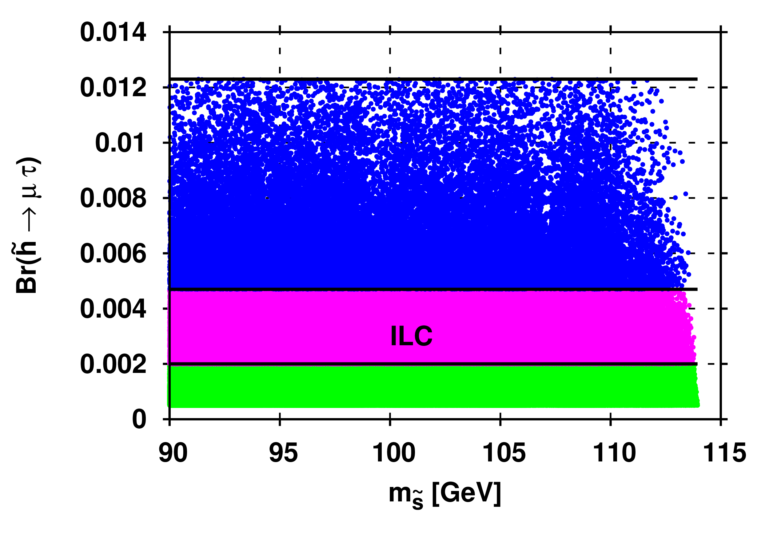
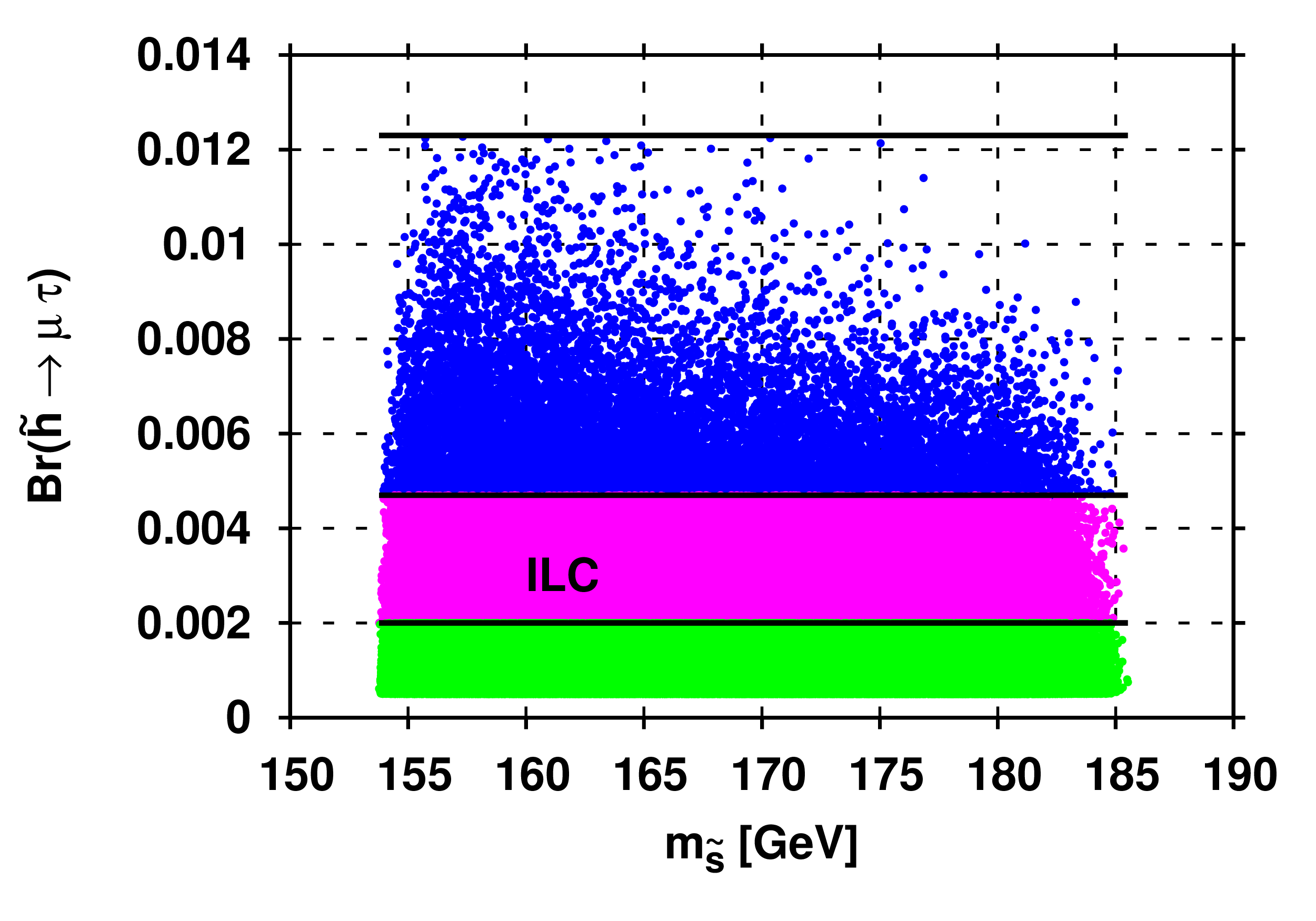
Figure 6: Scatter plots in plane $\left(m_{\tilde{s}},\text{Br}(\tilde{h}\to\tau\mu)\right)$ for $\sqrt{F}=8\leavevmode\nobreak\ \text{TeV}$ and sgoldstino lighter (left) and heavier (right) than Higgs.

for light (left panel) and heavy (right panel) sgoldstino. We find a lot of phenomenologically accepted models explaining the CMS excess. In Fig. 7 we present distribution of all the selected models in $\left(m_{\tilde{s}},\sqrt{\frac{A_{\tau\mu}^{2}+A_{\mu\tau}^{2}}{2F}}\right)$-plane for lighter (left panel) and heavier (right panel) sgoldstinos.

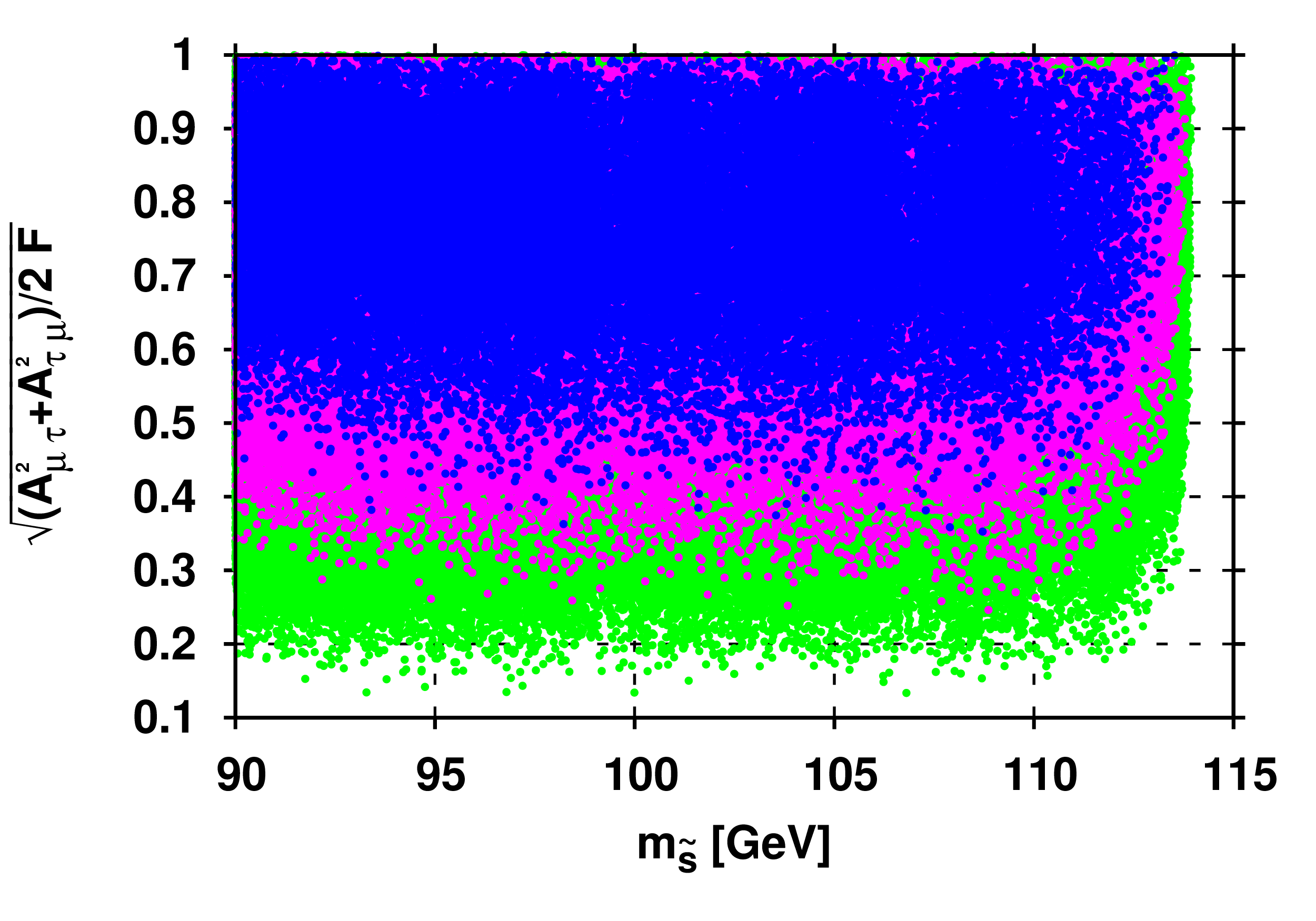
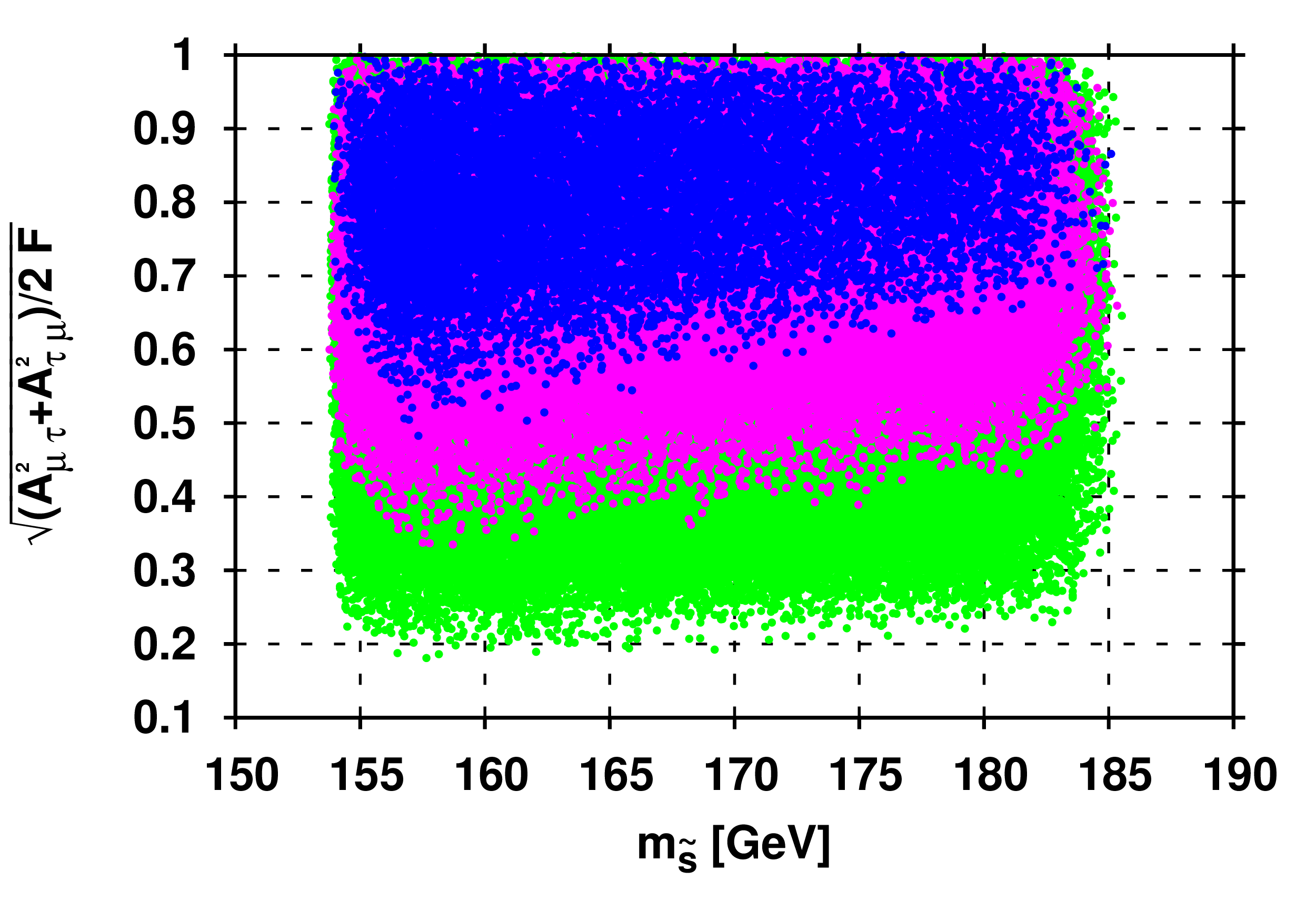
Figure 7: Scatter plots in plane $\left(m_{\tilde{s}},\sqrt{\frac{A_{\tau\mu}^{2}+A_{\mu\tau}^{2}}{2F}}\right)$ for $\sqrt{F}=8\leavevmode\nobreak\ \text{TeV}$ and sgoldstino lighter (left) and heavier (right) than than the Higgs boson. By color, we show different levels of ${\rm Br}(\tilde{h}\to\mu\tau)$ as in Fig. 6.

Sgoldstino explanation of the CMS excess requires large sgoldstino admixture in the Higgs boson and sufficiently large values of the soft trilinear coupling constants $A_{\mu\tau}$ and/or $A_{\tau\mu}$. This can present a problem for model building and we leave this question for future study. Numerically, we obtain that the value of $|\sin{\theta}|$ should be larger than 0.05 (0.15) for light (heavy) sgoldstino for models with ${\rm Br}(\tilde{h}\to\tau\mu)>5\cdot 10^{-4}$. Now let us comment more on the choice of the sgoldstino mass intervals and the value of supersymmetry breaking scale. It appears that sgoldstino with masses larger than about 200 GeV is not capable to explain the CMS excess in chosen parameter space (see Table 1). Larger sgoldstino masses result in a suppression of the mixing angle (see eq. (2.13)) and correspondingly in a decrease of ${\rm Br}(\tilde{h}\to\mu\tau)$ below the values indicated by the CMS excess. At the same time, values of $\sqrt{F}$ smaller than about $8$ TeV also turn out to be disfavored by this excess and results of direct searches. Namely, at smaller $\sqrt{F}$ the coupling constants of sgoldstino to the SM particles increase and such sgoldstino is phenomenologically unacceptable. In this case, very light sgoldstino, which decays mostly to $b\macc@depth\char 1\relax\frozen@everymath{\macc@group}\macc@set@skewchar\macc@nested@a 111{b}$ due to large mixing with the Higgs boson, becomes excluded by the TeVatron and LEP results. Heavier sgoldstino with $\sqrt{F}$ smaller than about 8 TeV is excluded by the results of the ATLAS and CMS searches for diboson resonances. If we enlarge our parameter space by increasing, in particular, the upper bound on $\mu$ in the Table 1, we expect that somewhat lower values of $\sqrt{F}$ and larger values of the sgoldstino mass will be allowed.

In Fig. 8

Figure 8: Scatter plots in plane $\left(\mu_{\gamma\gamma},\mu_{\scriptscriptstyle VV}\right)$ for $\sqrt{F}=8\leavevmode\nobreak\ \text{TeV}$ and sgoldstino lighter (left) and heavier (right) than the Higgs boson. By color, we show different levels of ${\rm Br}(\tilde{h}\to\mu\tau)$ as in Fig. 6.

we show the selected models in $\left(\mu_{\gamma\gamma},\mu_{\scriptscriptstyle VV}\right)$-plane for light (left panel) and heavy (right panel) sgoldstino. Here $\mu_{\scriptscriptstyle VV}$ is either $\mu_{ZZ}$ or $\mu_{WW}$ (they are almost coincide for our choice of parameters). For the case of lighter sgoldstinos, two disjoint regions correspond to the opposite signs of parameter $\mu$. In the case of heavier sgoldstinos, only positive values of $\mu$ are phenomenologically allowed. The deviation of $\mu_{\scriptscriptstyle VV}$ with respect to their SM values occurs mainly as a results of an increase in the Higgs-gluon coupling constant, because for the chosen parameter space couplings of sgoldstino to massive vector bosons and $b$-quarks are smaller than those of the Higgs boson. The Standard Model Higgs boson interacts with massless gauge bosons via loops only. This results in a possibility that the couplings $g_{hgg,\rm{SM}}$ and $g_{sgg}$ can be of the same order. Estimates show that one has $\mu_{\scriptscriptstyle VV}<1\,(>1)$ when $\mu>0\,(\mu<0)$ for $m_{\tilde{s}}<m_{\tilde{h}}$.

Sgoldstino-Higgs mixing results also in changes of the signal strengths for fermionic final states. For chosen parameter space, the coupling constants of sgoldstino to $\tau$-leptons and $b$-quarks are comparable with corresponding couplings of the Higgs boson, while for muons can even exceed it. For an illustration, in Fig. 9 we show the scatter plot in $\left(\mu_{\tau\tau}^{{\rm VBF}},\mu_{\tau\tau}^{{\rm ggF}}\right)$-plane for $\tau^{+}\tau^{-}$ final state. Here the modifications of the signal strengths are mainly due to changes in the production cross section and the total width of the Higgs resonance. Again, disjoint regions for $\mu_{\tau\tau}^{\rm ggF}$ correspond to different signs of $\mu$.

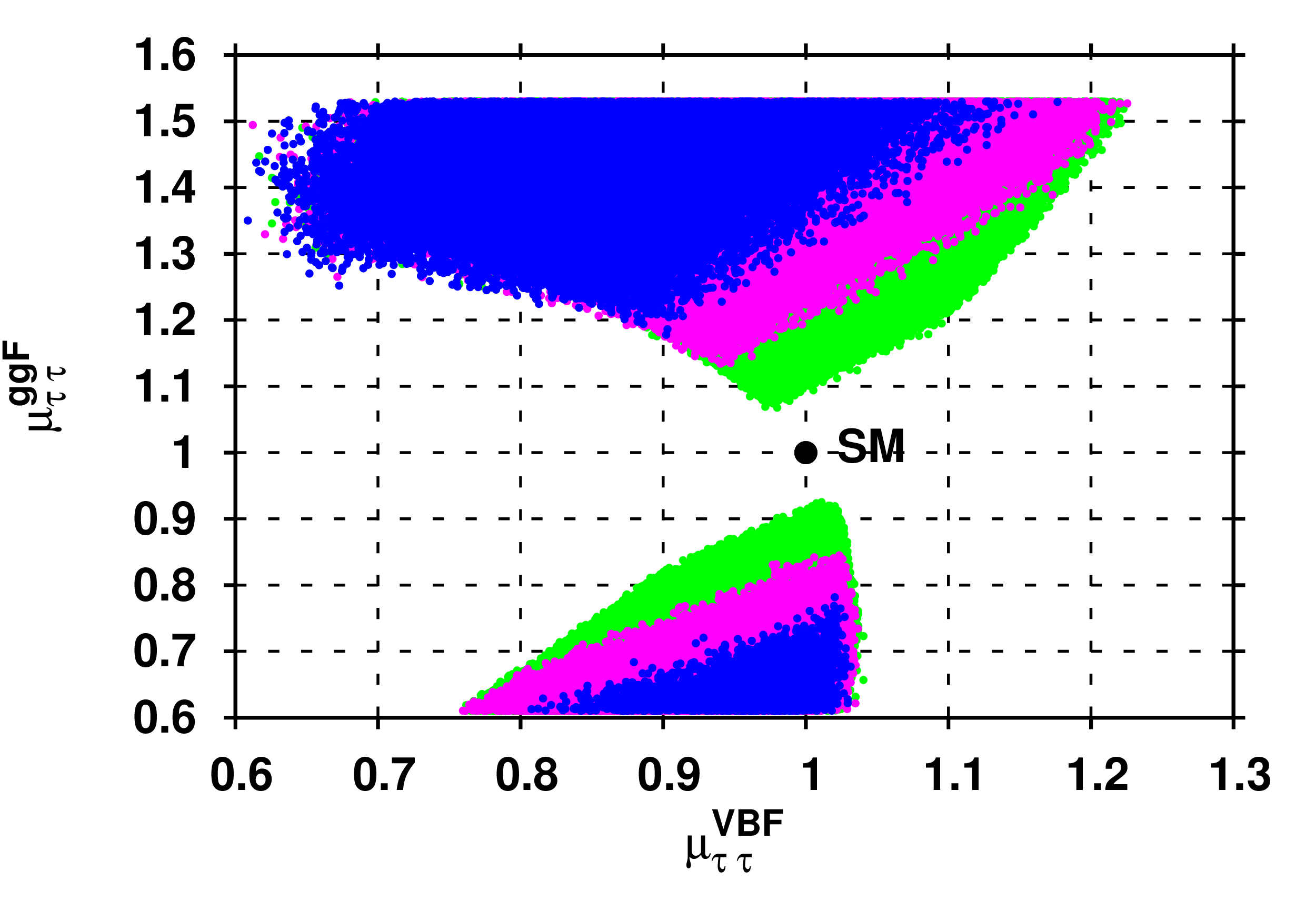
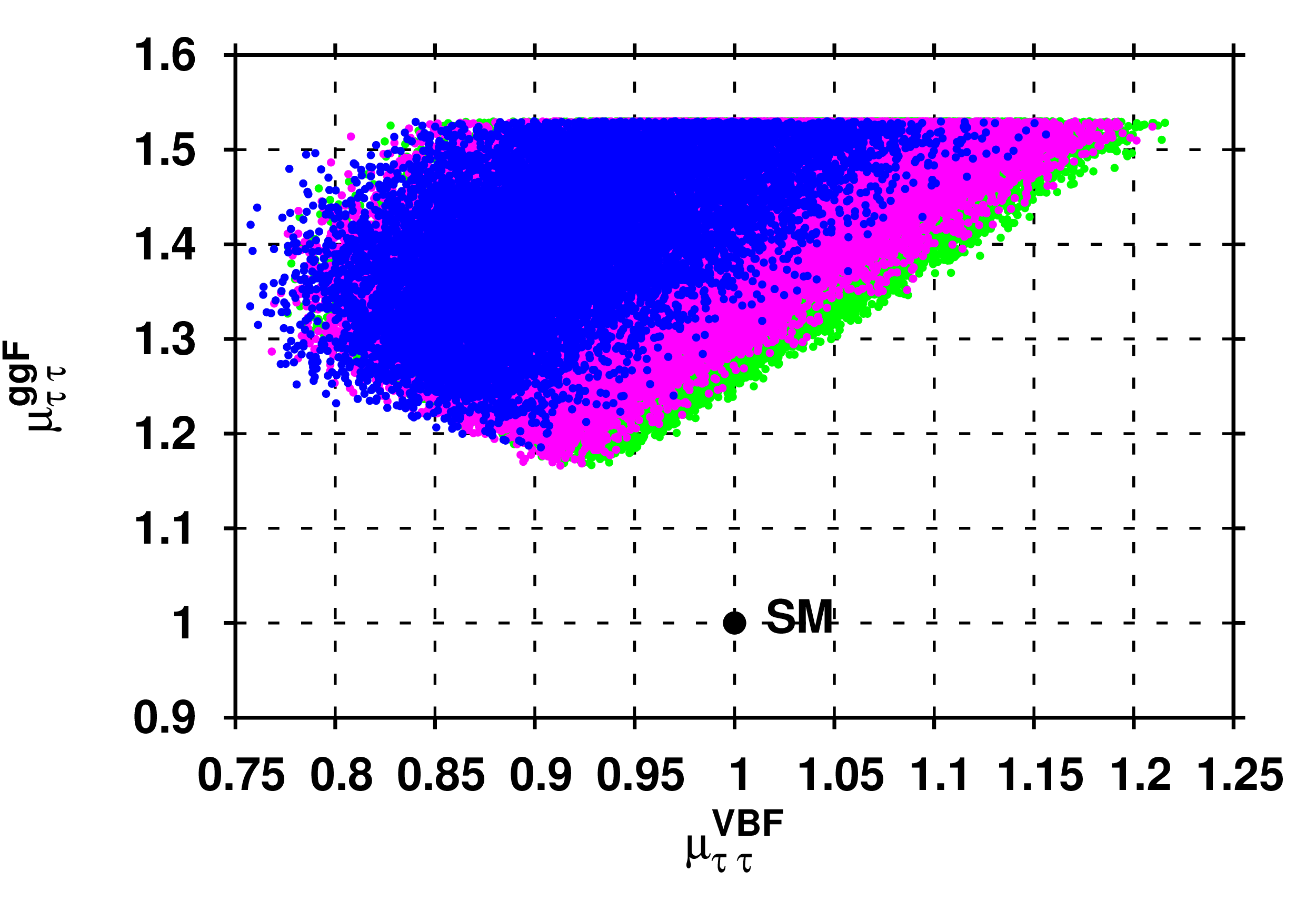
Figure 9: Scatter plots in plane $\left(\mu_{\tau\tau}^{{\rm VBF}},\mu_{\tau\tau}^{{\rm ggF}}\right)$ for $\sqrt{F}=8\leavevmode\nobreak\ \text{TeV}$ and sgoldstino lighter (left) and heavier (right) than the Higgs boson. By color, we show different levels of ${\rm Br}(\tilde{h}\to\mu\tau)$ as in Fig. 6.

In figure  10

Figure 10: Scatter plots in plane $\left(\mu_{\mu\mu}^{{\rm VBF}},\mu_{\mu\mu}^{{\rm ggF}}\right)$ for $\sqrt{F}=8\leavevmode\nobreak\ \text{TeV}$ and sgoldstino lighter (left) and heavier (right) than the Higgs boson. By color, we show different levels of ${\rm Br}(\tilde{h}\to\mu\tau)$ as in Fig. 6.

we show the scatter plots in plane $\left(\mu_{\mu\mu}^{{\rm VBF}},\mu_{\mu\mu}^{{\rm ggF}}\right)$ for $\mu^{+}\mu^{-}$ final state. In this case the main change is due to considerable modification of the Higgs boson coupling to muons. For the case of light sgoldstino and $\mu>0$, this enhancement can be partially compensated by a suppression of the production cross section and corresponding models lie on the thin line in the low part of the left panel in the figure 10.

Now let us discuss the collider phenomenology of the light sgoldstino. This scalar can reveal itself in the experiments at the LHC as a diboson resonance. In the case of large $\sqrt{F}$ and sufficiently large mixing of sgoldstino with the Higgs boson, the decay pattern of sgoldstino becomes similar to that of the Higgs boson. It means that for heavier sgoldstino the most important decay channels will be $W^{+}W^{-}$ and $ZZ$. Corresponding cross sections $\sigma\left(pp\to\tilde{s}\right)\times{\rm Br}\left(\tilde{s}\to W^{+}W^{-}\;{\rm or}\;ZZ\right)$ are presented in Fig. 11

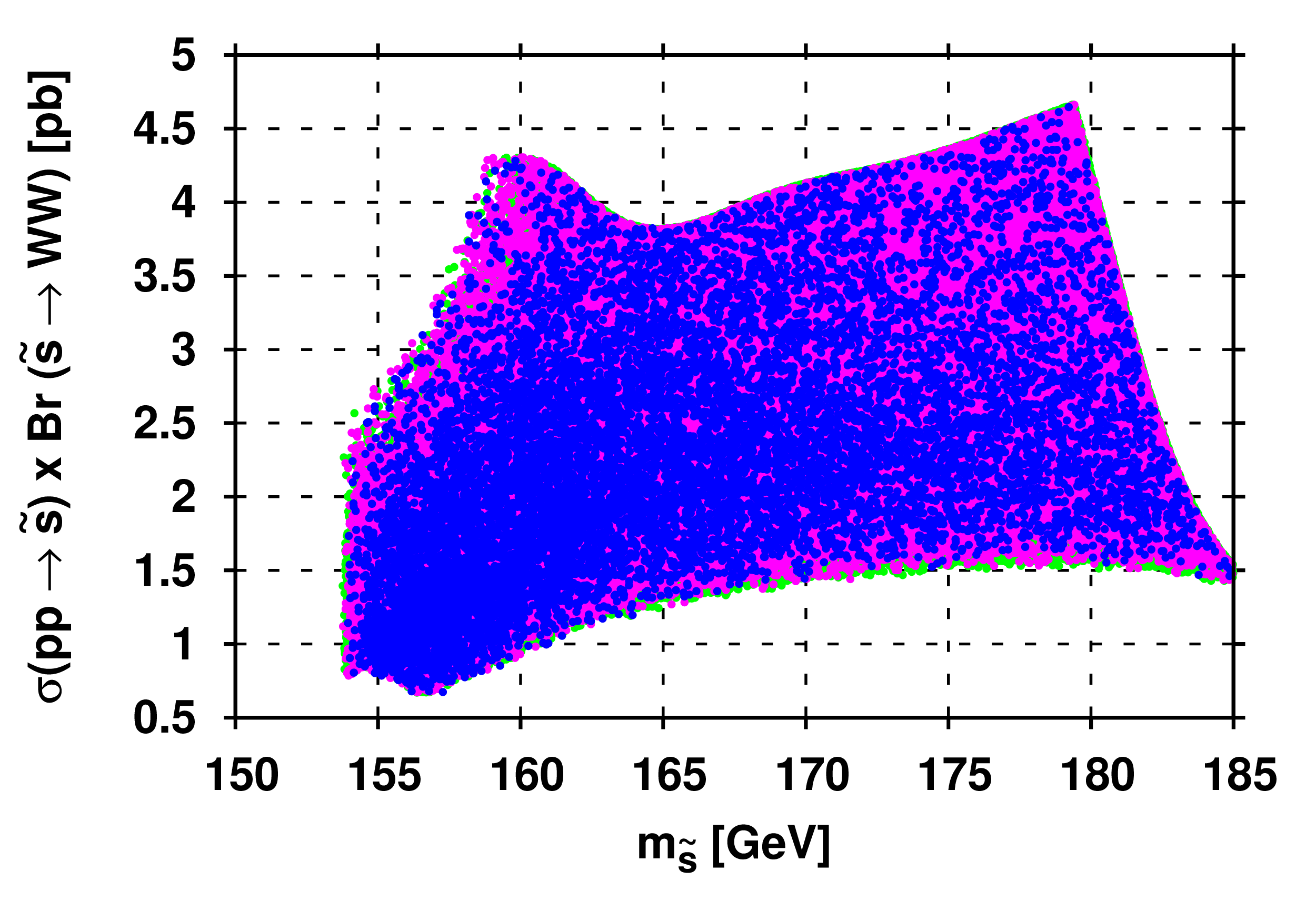
Figure 11: Scatter plots in $\sigma\left(pp\to\tilde{s}\right)\times{\rm Br}\left(\tilde{s}\to W^{+}W^{-}\;{\rm or}\;ZZ\right)$-plane for heavy sgoldstino and $\sqrt{s}=13$ TeV. By color we show different levels of ${\rm Br}(\tilde{h}\to\mu\tau)$ as in Fig. 6.

for the case of $\sqrt{s}=13$ TeV. Upper envelopes at these scatter plots correspond to the current upper limits from diboson searches at the LHC. We see that predicted cross sections reach values about several picobarns for $WW$ final state and values of about 0.2 pb for $ZZ$ case which can be explored in the starting LHC run. Another important decay channel for heavier sgoldstino is decay into a pair of photons. We calculated corresponding expected cross-section for $\sqrt{s}=13$ TeV. The result is presented on the right panel of Fig.12.

Figure 12: Scatter plots in $\sigma\left(pp\to\tilde{s}\right)\times{\rm Br}\left(\tilde{s}\to\gamma\gamma\right)$-plane for light (left panel) and heavy (right panel) sgoldstino and $\sqrt{s}=13$ TeV. By color we show different levels of ${\rm Br}(\tilde{h}\to\mu\tau)$ as in Fig. 6.

Obtained values reaching 0.01–0.1 pb seem to be promising quite since they can be verified in the next run of the LHC, especially for heavy sgoldstino. Sgoldstino of lower masses with sufficiently large Higgs boson admixture decays mainly to $b\bar{b}$ but this mass region seems to be quite difficult to probe with such final state at the ATLAS and CMS experiments. At the same time, in the considered scenario the scalar sgoldstino have large flavor-violating $\mu$–$\tau$ coupling and thus considerable branching fraction of $\tilde{s}\to\mu\tau$ decay. In Fig. 13

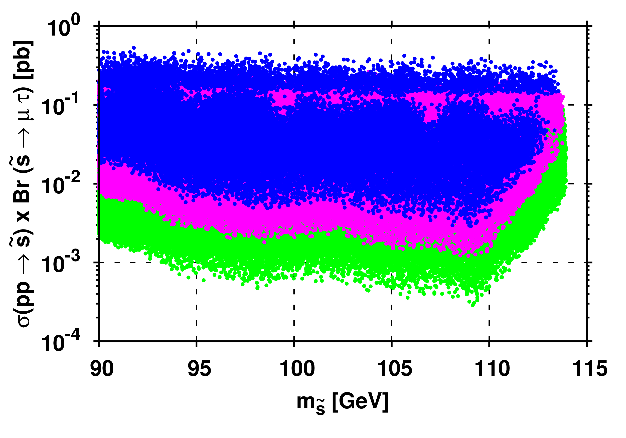
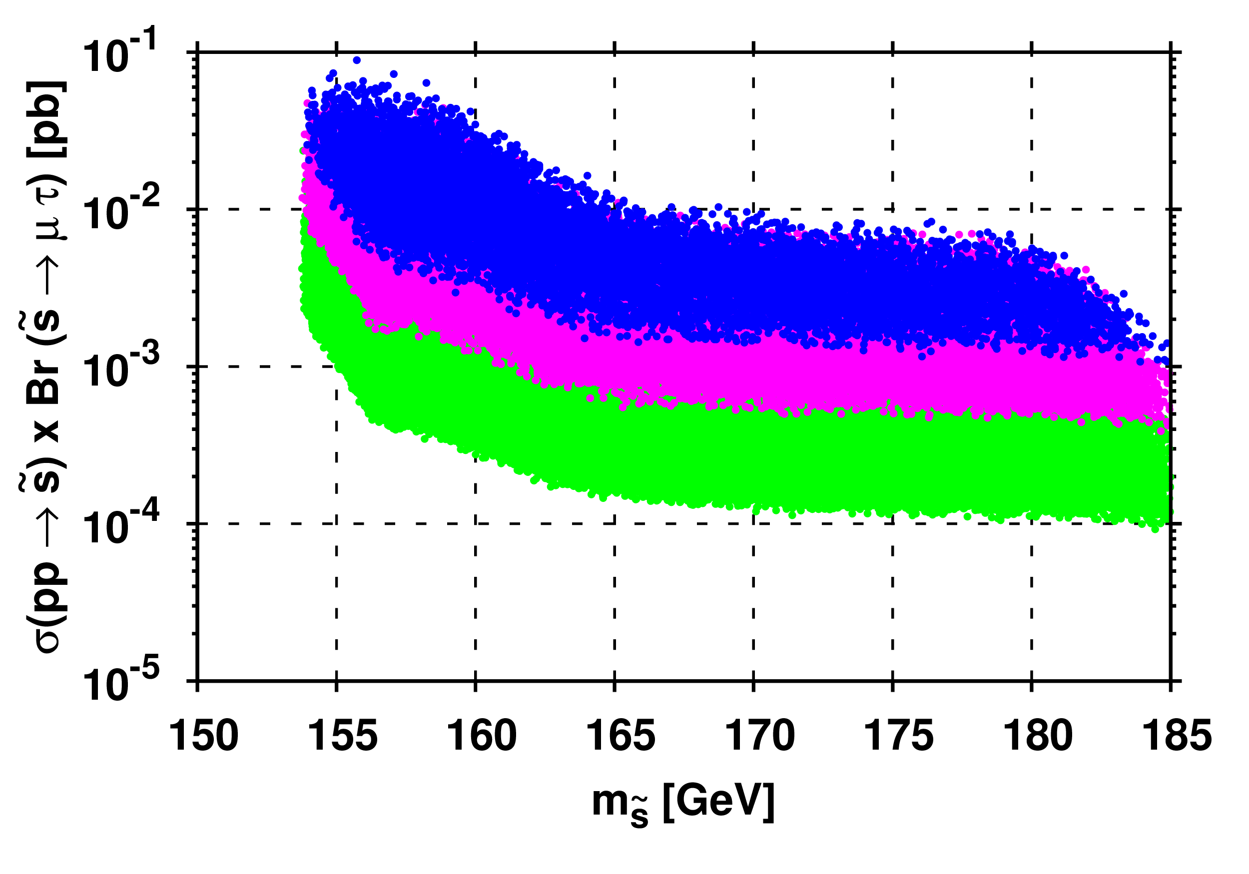
Figure 13: Scatter plots in ($m_{\tilde{s}}$, $\sigma(pp\to\tilde{s})\times{\rm Br}(\tilde{s}\to\mu\tau)$)-plane for different masses of sgoldstino and $\sqrt{s}=13$ TeV. By color we show different levels of ${\rm Br}(\tilde{h}\to\mu\tau)$ as in Fig. 6.

we show the cross section $\sigma\left(pp\to\tilde{s}\right)\times{\rm Br}\left(\tilde{s}\to\mu\tau\right)$ calculated at $\sqrt{s}=13$ TeV for selected models and different sgoldstino masses. We see that it reaches values about 0.1–0.2 pb for models explaining the CMS excess, which hopefully can be probed in the next runs of the LHC experiments.

Finally, in Fig. 14 we present predictions for ${\rm Br}\left(\tau\to\mu\gamma\right)$ and ${\rm Br}\left(\tau\to 3\mu\right)$ in the model with sgoldstino.

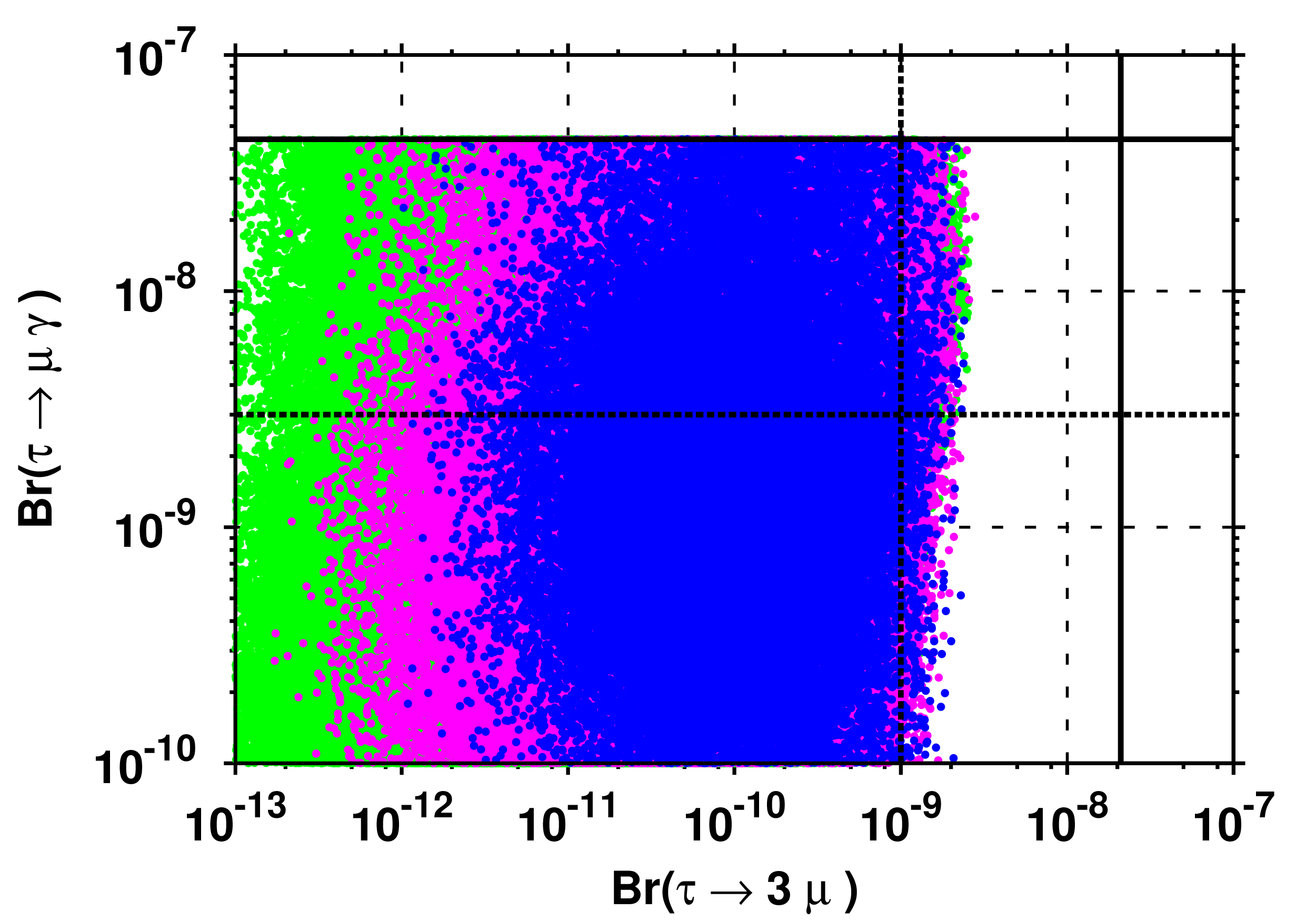
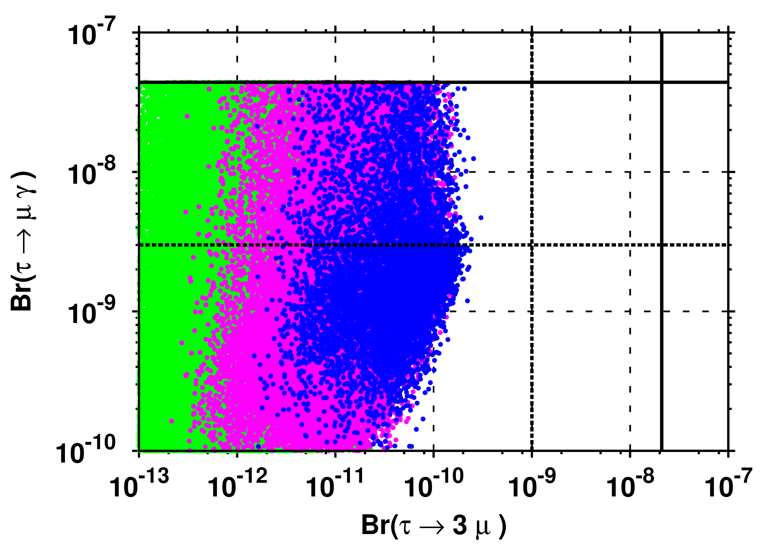
Figure 14: Scatter plots in plane $\left(\text{Br}(\tau\to\mu\gamma),\text{Br}(\tau\to 3\mu)\right)$ for $\sqrt{F}=8\leavevmode\nobreak\ \text{TeV}$ and sgoldstinos lighter (left) and heavier (right) than the Higgs boson. Solid lines correspond to present limits on branching fraction of both decays, whereas dashed line represents expected SuperKEKB sensitivity Aushev:2010bq . By color we show different levels of ${\rm Br}(\tilde{h}\to\mu\tau)$ as in Fig. 6.

As we discussed in the previous section, our effective low energy theory has limited predictive power for such observables and in the present study they are only estimated using realistic value of the cutoff for dominant divergent loop diagrams, $\Lambda^{2}=16\pi F^{2}/m_{\text{sl}}^{2}$ (see Appendix B and Refs. Brignole:2000wd ; Brignole:1998uu ; Brignole:1996fn ). The dominant contribution to ${\rm Br}(\tau\to\mu\gamma)$ comes from the standard one-loop diagram with sfermions while for ${\rm Br}(\tau\to 3\mu)$ we leave only the tree-level contribution with sgoldstino and Higgs boson exchange. In Fig. 14 by solid lines we show the current experimental bounds, while the dashed lines show the expected SuperKEKB sensitivities to these decays Aushev:2010bq . We checked that with another choice of the cutoff scale, for instance, $\Lambda=\sqrt{F}$ or $\Lambda=m_{sl}$, the predictions for the rate of $\tau\to\mu\gamma$ decay for each particular model in the parameter space can differ considerably. But the whole picture of colored points on Fig. 14 remains almost unchanged. Thus, our analysis reveals the level of ${\rm Br}(\tau\to\mu\gamma)$ about $10^{-8}$ can expected in the considered setup. We see that many models with low scale supersymmetry breaking explaining the CMS excess can be possibly probed by these searches. However, we should stress that knowledge of particular microscopic theory is needed to make more solid predictions for ${\rm Br}(\tau\to\mu\gamma)$ and ${\rm Br}(\tau\to 3\mu)$ for a particular point in the parameter space.

5 Conclusions

In this paper we showed that in models with scale of supersymmetry breaking around several TeVs and having superlight singlet goldstino and relatively light sgoldstinos (with the latter’s masses around hundreds GeVs), the Higgs boson can have considerable branching ratio of $h\to\tau\mu$ decay. In particular, we demonstrated that the CMS excess in $h\to\tau\mu$ decay can be explained in this framework. This interesting scenario involves nonzero mixing of the lightest Higgs boson with scalar sgoldstino which can have flavor-violating couplings to SM fermions. We stress, that these features are common in the class of models in question.

We performed a scan over relevant parameter space of the model and found several distinct signatures of this scenario. First of all, due to the mixing with sgoldstino, considerable changes of the Higgs boson signal strengths for the main search channels $\gamma\gamma$, $ZZ$, $W^{+}W^{-}$, $\tau^{+}\tau^{-}$ and $\mu^{+}\mu^{-}$ are expected as compared to the SM predictions. We find that for most of the models explaining the CMS excess the signal strengths differ by more than 10% from the SM predictions for gluon-gluon fusion production mechanism and even more for the case of $\mu^{+}\mu^{-}$ final state. Also, in our setup new scalar light state, sgoldstino, with its mass not very far from that of the Higgs resonance is present in the particle spectrum. It can reveal itself in proton collisions at the LHC decaying into the final states similar to what happens to the Higgs boson. The scalar sgoldstino can be effectively probed in searches for diboson resonances in the recently started LHC run. Predicted values of the corresponding cross sections are presented in figures 11 and 12. Moreover, the scalar sgoldstino have also considerable flavor-violating decay with $\mu\tau$ final state. Predictions for LFV decays $\tau\to\mu\gamma$ and $\tau\to 3\mu$ within models with low scale supersymmetry breaking are plagued from uncertainties related to precise knowledge of microscopic theory. Using some simplifying assumptions and realistic value for the cutoff of the effective theory we made an estimate for branching ratios of these decays and found obtained values to be interesting in a part of the parameter space for the nearest future experiments in this area.

Here we concentrated on lepton flavor violation in $\mu-\tau$ sector motivated by the CMS results. However, we note that sgoldstino-Higgs mixing as well as (lepton) flavour violation in sgoldstino interactions are rather general predictions of low scale supersymmetry. Hence, the model with light goldstino sector can result in LFV Higgs boson decay $h\to\tau e$ at similar level as predicted for $h\to\tau\mu$.

Acknowledgements.

We thank D. Gorbunov for useful discussions. This work is supported by the RSCF grant 14-22-00161. Numerical calculations have been performed on the Computational cluster of the Theoretical division of INR RAS.

Appendix A Coupling constants of $\tilde{h}$ and $\tilde{s}$.

In this Appendix, we present relevant expressions for the modified coupling constants of the Higgs and sgoldstino mass states, as well as their decay rates. In the decoupling limit of the MSSM, we are left with the lightest Higgs boson with the following relevant effective interactions

$$\mathcal{L}_{h}^{eff}=g_{h\gamma\gamma}\,hF_{\mu\nu}F^{\mu\nu}+g_{hgg}h\,\text{tr}\,G_{\mu\nu}G^{\mu\nu}-\frac{m_{b}}{\sqrt{2}v}\,h\macc@depth\char 1\relax\frozen@everymath{\macc@group}\macc@set@skewchar\macc@nested@a 111{b}b+\frac{\sqrt{2}m_{W}^{2}}{v}\,hW_{\mu}^{+}W^{\mu-}+\frac{\sqrt{2}m_{Z}^{2}}{2v}\,hZ_{\mu}Z^{\mu},$$ (A.1)

where $g_{h\gamma\gamma}$ and $g_{hgg}$ are the loop factors. Interactions between scalar sgoldstino and the SM gauge bosons and fermions are given by

$$\mathcal{L}_{s}^{eff}=-\frac{M_{\gamma\gamma}}{2\sqrt{2}}\,s\,F_{\mu\nu}F^{\mu\nu}-\frac{M_{3}}{2\sqrt{2}F}\,s\,\text{tr}\,G_{\mu\nu}G^{\mu\nu}+\frac{A_{bb}\,v_{d}}{\sqrt{2}F}s\macc@depth\char 1\relax\frozen@everymath{\macc@group}\macc@set@skewchar\macc@nested@a 111{b}b-\frac{M_{2}}{\sqrt{2}F}\,s\,W_{\mu\nu}W^{\mu\nu*}-\frac{M_{ZZ}}{2\sqrt{2}F}\,s\,Z_{\mu\nu}Z^{\mu\nu},$$ (A.2)

where

$$\begin{aligned} &M_{ZZ}=M_{1}\,\sin^{2}\theta_{W}+M_{2}\,\cos^{2}\theta_{W}\,,\\ &M_{\gamma\gamma}=M_{1}\,\cos^{2}\theta_{W}+M_{2}\,\sin^{2}\theta_{W}.\end{aligned}$$ (A.3)

The effective interactions with photons, gluons and SM fermions have the same form for the Higgs boson $h$ and sgoldstino $s$. As a consequence, corresponding coupling constants for the mass state $\tilde{h}$ will be given by the following combinations

$$g_{\tilde{h}\gamma\gamma}=g_{h\gamma\gamma,\text{SM}}^{\text{1-loop}}\,\cos\theta+\frac{M_{\gamma\gamma}}{2\sqrt{2}F}\,\sin\theta\,,$$ (A.4)

$$g_{\tilde{h}gg}=g_{hgg,\text{SM}}^{\text{1-loop}}\,\cos\theta+\frac{M_{3}}{2\sqrt{2}F}\,\sin\theta$$ (A.5)

for photons and gluons and

$$\begin{aligned} &Y_{\tau\tau}^{\tilde{h}}=\frac{m_{\tau}}{\sqrt{2}v}\,\cos\theta+\frac{A_{\tau\tau}\,v\,\cos\beta}{\sqrt{2}F}\,\sin\theta\,,\\ &Y_{bb}^{\tilde{h}}=\frac{m_{b}}{\sqrt{2}v}\,\cos\theta+\frac{A_{bb}\,v\,\cos\beta}{\sqrt{2}F}\,\sin\theta\,,\\ &Y_{\mu\mu}^{\tilde{h}}=\frac{m_{\mu}}{\sqrt{2}v}\,\cos\theta+\frac{A_{\mu\mu}\,v\,\cos\beta}{\sqrt{2}F}\,\sin\theta\\ \end{aligned}$$ (A.6)

for SM fermions. The loop factors look as follows Spira:1997dg

$$\begin{aligned} &g_{\text{h}\gamma\gamma,\text{SM}}^{\text{1-loop}}=\frac{\alpha}{8\sqrt{2}\pi v}\left(A_{1}(\tau_{W})+\sum_{q}N_{c}\,Q_{q}^{2}\,A_{1/2}(\tau_{q})\right)\,,\\ &g_{\text{h}gg,\text{SM}}^{\text{1-loop}}=\frac{\alpha_{s}}{16\sqrt{2}\pi v}\sum_{q}A_{1/2}(\tau_{q}),\end{aligned}$$ (A.7)

where $A_{1}$ and $A_{1/2}$ are boson and fermion contributions, respectively,

$$\begin{aligned} &A_{1}(\tau)=-(2+3\tau+3\tau(2-\tau)f(\tau))\,,\\ &A_{1/2}(\tau)=2\tau(1+(1-\tau)f(\tau))\end{aligned}$$ (A.8)

and

$$\begin{aligned} &f(\tau)=\left\{\begin{aligned} &\arcsin^{2}\left(\frac{1}{\sqrt{\tau}}\right),&\quad\tau\geq 1\\ &-\frac{1}{4}\left[\log\frac{1+\sqrt{1-\tau}}{1-\sqrt{1-\tau}}-\dot{\imath}\,\pi\right]^{2},&\quad\tau<1\end{aligned}\right.\end{aligned}$$ (A.9)

with $\displaystyle\tau_{i}=\frac{4m_{i}^{2}}{m_{h}^{2}}$. Corresponding decay widths can be written as

$$\Gamma(\tilde{h}\rightarrow\gamma\gamma)=\frac{G_{\scriptscriptstyle F}\alpha^{2}m_{\tilde{h}}^{3}}{128\sqrt{2}\pi^{3}}\left|\left(A_{1}(\tau_{W})+\sum_{q}N_{c}\,Q_{q}^{2}\,A_{1/2}(\tau_{q})\right)\cos\,\theta+\frac{4M_{\gamma\gamma}v\pi}{\alpha F}\sin\,\theta\right|^{2}\,,$$ (A.10)

$$\Gamma(\tilde{h}\rightarrow gg)=\frac{\alpha_{s}^{2}\,m_{\tilde{h}}^{3}\,G_{\scriptscriptstyle F}}{36\sqrt{2}\pi^{3}}\left|\sum_{q}\frac{3}{4}A_{1/2}(\tau_{q})\,\cos\theta+\frac{6M_{3}\pi v}{\alpha_{s}\,F}\,\sin\theta\right|^{2}\,,$$ (A.11)

$$\Gamma(\tilde{h}\rightarrow\macc@depth\char 1\relax\frozen@everymath{\macc@group}\macc@set@skewchar\macc@nested@a 111{f}f)=\frac{m_{\tilde{h}}\,(Y_{ff}^{\tilde{h}})^{2}}{8\pi}\left(1-\frac{4m_{f}^{2}}{m_{\tilde{h}}^{2}}\right)^{\frac{3}{2}}\,.$$ (A.12)

The case of interaction with $W$ and $Z$ bosons is more involved, because of different type of operators in Eqs. (A.1),(A.2). Corresponding couplings for $\tilde{h}$ can be conveniently written in the momentum space as follows

$$g_{\tilde{h}VV}^{\mu\nu}=g_{hVV}^{\mu\nu}\cos\theta+\frac{M_{VV}}{\sqrt{2}F}\left((k_{V_{1}},k_{V_{2}})\eta^{\mu\nu}-k^{V_{1}\mu}k^{V_{2}\nu}\right)\sin\theta,$$ (A.13)

where

$$g_{hVV}^{\mu\nu}=\frac{2m_{V}^{2}}{v}\eta^{\mu\nu}$$ (A.14)

and $M_{VV}$ is either $M_{2}$ or $M_{ZZ}$ for $W$ and $Z$ bosons, respectively. The expression for the decay width Romao:1998sr which takes into account possibility of the virtual massive vector boson production looks as

$$\begin{aligned} \Gamma(\tilde{h}\rightarrow V^{*}V^{*}\rightarrow\text{leptons})=\frac{1}{\pi}&\int_{0}^{m_{\tilde{h}}^{2}}\,d\Delta_{i}^{2}\frac{\Gamma_{V}M_{V}}{|D(\Delta_{i}^{2})|^{2}}\frac{1}{\pi}\\ &\times\int_{0}^{\left(m_{\tilde{h}}-\sqrt{\Delta_{i}^{2}}\right)^{2}}\,d\Delta_{j}^{2}\frac{\Gamma_{V}M_{V}}{|D(\Delta_{j}^{2})|^{2}}\,\Gamma_{0}^{V}(\Delta_{i},\Delta_{j},m_{\tilde{h}},\theta),\end{aligned}$$ (A.15)

where

$$\begin{aligned} \Gamma_{0}^{V}(\Delta_{i},\Delta_{j},m_{\tilde{h}},\theta)=\delta_{V}\frac{Gm_{\tilde{h}}^{3}}{16\pi\sqrt{2}}\sqrt{\lambda(\Delta_{i}^{2},\Delta_{j}^{2},m_{\tilde{h}}^{2})}\Biggl{[}&\cos^{2}\theta\left(\lambda(\Delta_{i},\Delta_{j},m_{\tilde{h}})+12\frac{\Delta_{i}^{2}\Delta_{j}^{2}}{m_{\tilde{h}}^{4}}\right)\\ &+X(\Delta_{i}^{2},\Delta_{j}^{2},\theta)\Biggr{]},\end{aligned}$$

$$D(\Delta^{2})=\Delta^{2}-m_{V}^{2}+\dot{\imath}m_{V}\,\Gamma_{V},$$

$$\lambda(\Delta_{i}^{2},\Delta_{j}^{2},m_{\tilde{h}}^{2})=\left(1-\frac{\Delta_{i}^{2}}{m_{\tilde{h}}^{2}}-\frac{\Delta_{j}^{2}}{m_{\tilde{h}}^{2}}\right)^{2}-4\frac{\Delta_{i}^{2}\Delta_{j}^{2}}{m_{\tilde{h}}^{4}}\,,$$ (A.16)

$$\begin{aligned} X(\Delta_{i}^{2},\Delta_{j}^{2},\theta)=\frac{\Delta_{i}^{2}\Delta_{j}^{2}}{m_{\tilde{h}}^{4}}\,\Omega\,\sin\theta\Biggl{[}&12\cos\theta\left(-\Delta_{i}^{2}-\Delta_{j}^{2}+m_{\tilde{h}}^{2}\right)+\\ &4\leavevmode\nobreak\ \Omega\leavevmode\nobreak\ \sin\theta\left(\frac{\left(\Delta_{i}^{2}+\Delta_{j}^{2}-m_{\tilde{h}}^{2}\right)^{2}}{2}+\Delta_{i}^{2}\,\Delta_{j}^{2}\right)\Biggr{]}\end{aligned}$$

and $\Omega=\displaystyle\frac{M_{\scriptscriptstyle{VV}}v}{F}$. In formulas (A.16), $\delta=1(2)$ for $Z(W)$ bosons and $\Delta_{i,j}$ is a four-momentum of off-shell particles $V^{*}$.

The same expressions (A.15) and (A.16) for decay widths are applied for sgoldstinos with the substitutions $\cos\theta\rightarrow\sin\theta$ and $\sin\theta\rightarrow-\cos\theta$.

Appendix B Contributions to $\tau\to\mu\gamma$ decay

In this Appendix, we present expressions for different contributions to the Wilson coefficients $c_{L}$ and $c_{R}$ in Eq (3.6) which we use to estimate the branching ratio of $\tau\to\mu\gamma$ decay. We start with the standard SUSY part arising from slepton sector (see Fig 4) which numerically gives dominant contribution for almost all models selected in our scan. The $6\times 6$ slepton squared mass matrix in electroweak interaction basis ($\tilde{e}_{L},\,\tilde{\mu}_{L},\,\tilde{\tau}_{L},\,\tilde{e}_{R},\,\tilde{\mu}_{R},\,\tilde{\tau}_{R}$) can be written in terms of 3 non-diagonal $3\times 3$ matrices Arana-Catania:2013ggc

$$M_{\tilde{l}}^{2}=\left(\begin{matrix}M_{\tilde{l}LL}^{2}&M_{\tilde{l}LR}^{2}\\ M_{\tilde{l}RL}^{2\dagger}&M_{\tilde{l}RR}^{2}\\ \end{matrix}\right),$$ (B.1)

where

$$\begin{aligned} &M_{\tilde{l}LLij}^{2}=m_{\tilde{L}ij}^{2}+\left(m_{l_{i}}^{2}+\left(\sin^{2}\theta_{W}-\frac{1}{2}\right)M_{Z}^{2}\,\cos 2\beta\right)\,\delta_{ij},\\ &M_{\tilde{l}RRij}^{2}=m_{\tilde{E}ij}^{2}+(m_{l_{i}}^{2}-\sin^{2}\theta_{W}\,M_{Z}^{2}\,\cos 2\beta)\,\delta_{ij},\\ &M_{\tilde{l}LRij}^{2}=v_{d}\,A_{ij}-m_{l_{i}}\,\mu\,\tan\beta\,\delta_{ij}.\end{aligned}$$ (B.2)

The matrices $m_{\tilde{L}}$, $m_{\tilde{E}}$, $A$ can be parametrized as

$$\begin{aligned} &m_{\tilde{L}}^{2}=\left(\begin{matrix}m_{\tilde{L}_{1}}^{2}&\delta_{12}^{LL}\,m_{\tilde{L}_{1}}m_{\tilde{L}_{2}}&\delta_{13}^{LL}\,m_{\tilde{L}_{1}}m_{\tilde{L}_{3}}\\ \delta_{21}^{LL}m_{\tilde{L}_{2}}m_{\tilde{L}_{1}}&m_{\tilde{L}_{2}}^{2}&\delta_{23}^{LL}\,m_{\tilde{L}_{2}}m_{\tilde{L}_{3}}\\ \delta_{31}^{LL}m_{\tilde{L}_{3}}m_{\tilde{L}_{1}}&\delta_{32}^{LL}\,m_{\tilde{L}_{3}}m_{\tilde{L}_{2}}&m_{\tilde{L}_{3}}^{2}\\ \end{matrix}\right),\\ \\ &v_{d}\,A=\left(\begin{matrix}m_{e}\,A_{ee}&\delta_{12}^{LR}\,m_{\tilde{L}_{1}}m_{\tilde{E}_{2}}&\delta_{13}^{LR}\,m_{\tilde{L}_{1}}m_{\tilde{E}_{3}}\\ \delta_{21}^{LR}m_{\tilde{L}_{2}}m_{\tilde{E}_{1}}&m_{\mu}\,A_{\mu\mu}&\delta_{23}^{LR}\,m_{\tilde{L}_{2}}m_{\tilde{E}_{3}}\\ \delta_{31}^{LR}m_{\tilde{L}_{3}}m_{\tilde{E}_{1}}&\delta_{32}^{LR}\,m_{\tilde{L}_{3}}m_{\tilde{E}_{2}}&m_{\tau}\,A_{\tau\tau}\\ \end{matrix}\right),\\ \\ &m_{\tilde{E}}^{2}=\left(\begin{matrix}m_{\tilde{E}_{1}}^{2}&\delta_{12}^{RR}\,m_{\tilde{E}_{1}}m_{\tilde{E}_{2}}&\delta_{13}^{RR}\,m_{\tilde{E}_{1}}m_{\tilde{E}_{3}}\\ \delta_{21}^{RR}m_{\tilde{E}_{2}}m_{\tilde{E}_{1}}&m_{\tilde{E}_{2}}^{2}&\delta_{23}^{RR}\,m_{\tilde{E}_{2}}m_{\tilde{E}_{3}}\\ \delta_{31}^{RR}m_{\tilde{E}_{3}}m_{\tilde{E}_{1}}&\delta_{32}^{RR}\,m_{\tilde{E}_{3}}m_{\tilde{E}_{2}}&m_{\tilde{E}_{3}}^{2}\\ \end{matrix}\right).\end{aligned}$$ (B.3)

We assume that the LFV contribution comes from the trilinear couplings $A_{\mu\tau}$ and $A_{\tau\mu}$ only. Hence, we take $\delta_{ij}^{LL}=\delta_{ij}^{RR}=0$ for $i\neq j$ and also $\delta_{12}^{LR}=\delta_{21}^{LR}=\delta_{13}^{LR}=\delta_{31}^{LR}=0$. For simplicity, we assume a common mass scale $m_{\text{sl}}$ for right and left sleptons for all generations. Then we use general expression for contributions from SUSY particles obtained Arana-Catania:2013ggc ; Paradisi:2005fk in Mass Insertion Approximation

$$\begin{aligned} &c_{L}^{\text{SUSY}}=\frac{5\pi}{3}\frac{\alpha_{2}}{c_{\text{w}}^{2}}v\,A_{\tau\mu}\,\cos\beta\,\frac{M_{1}}{m_{\tau}}\frac{1}{m_{\tilde{R}}^{2}-m_{\tilde{L}}^{2}}\left(\frac{f_{3n}(a_{L})}{m_{\tilde{L}}^{2}}-\frac{f_{3n}(a_{R})}{m_{\tilde{R}}^{2}}\right)+\scriptstyle(\text{``LL contribution"}),\\ &c_{R}^{\text{SUSY}}=\frac{5\pi}{3}\frac{\alpha_{2}}{c_{\text{w}}^{2}}v\,A_{\mu\tau}\,\cos\beta\,\frac{M_{1}}{m_{\tau}}\frac{1}{m_{\tilde{R}}^{2}-m_{\tilde{L}}^{2}}\left(\frac{f_{3n}(a_{L})}{m_{\tilde{L}}^{2}}-\frac{f_{3n}(a_{R})}{m_{\tilde{R}}^{2}}\right)+\scriptstyle(\text{``RR contribution"}).\end{aligned}$$ (B.4)

In this expression, $m_{\tilde{L}}$ and $m_{\tilde{R}}$ are the average slepton masses in “left" and “right" sectors, respectively, $a_{\scriptstyle L,R}=\displaystyle\frac{M_{1}^{2}}{m_{\tilde{L},\tilde{R}}^{2}}$ and $f_{3n}$ is the loop function from neutralino contribution Arana-Catania:2013ggc ; Paradisi:2005fk

$$f_{3n}(a)=\frac{1+2a\,\log a-a^{2}}{2(1-a)^{3}}.$$ (B.5)

Using the simplifying assumptions discussed above and taking the limit $m_{\tilde{L}}^{2}-m_{\tilde{R}}^{2}\rightarrow 0$, the expression reduces to

$$\frac{1}{m_{\tilde{R}}^{2}-m_{\tilde{L}}^{2}}\left(\frac{f_{3n}(a_{L})}{m_{\tilde{L}}^{2}}-\frac{f_{3n}(a_{R})}{m_{\tilde{R}}^{2}}\right)\longrightarrow\frac{2f_{2n}(a)}{m_{\text{sl}}^{4}},$$ (B.6)

where $f_{2n}(a)$ is another neutralino loop function Arana-Catania:2013ggc

$$f_{2n}(a)=\frac{-5a^{2}+4a+1+2a(a+2)\log a}{4(1-a)^{4}}\,.$$ (B.7)

Now let us describe contributions from the diagrams with the Higgs boson and sgoldstino presented in Fig. 1. The leading order terms in the expansion in powers of $m_{\mu}/m_{\tilde{h}}$ ($m_{\mu}/m_{\tilde{s}}$) and $m_{\tau}/m_{\tilde{h}}$ ($m_{\tau}/m_{\tilde{s}}$) for the diagrams with internal Higgs-like state $\tilde{h}$ Harnik:2012pb are

$$\begin{aligned} &c_{L}^{\text{1-loop},\tilde{h}}\simeq\frac{1}{12\,m_{\tilde{h}}^{2}}Y_{\tau\tau}^{\tilde{h}}\,Y_{\tau\mu}^{\tilde{h}}\left(-4+3\log\frac{m_{\tilde{h}}^{2}}{m_{\tau}^{2}}\right)+\frac{1}{12\,m_{\tilde{h}}^{2}}Y_{\mu\mu}^{\tilde{h}}\,Y_{\tau\mu}^{\tilde{h}}\left(-4+3\log\frac{m_{\tilde{h}}^{2}}{m_{\mu}^{2}}\right)\,,\\ &c_{R}^{\text{1-loop},\tilde{h}}\simeq\frac{1}{12\,m_{\tilde{h}}^{2}}Y_{\tau\tau}^{\tilde{h}}\,Y_{\mu\tau}^{\tilde{h}}\left(-4+3\log\frac{m_{\tilde{h}}^{2}}{m_{\tau}^{2}}\right)+\frac{1}{12\,m_{\tilde{h}}^{2}}Y_{\mu\mu}^{\tilde{h}}\,Y_{\mu\tau}^{\tilde{h}}\left(-4+3\log\frac{m_{\tilde{h}}^{2}}{m_{\mu}^{2}}\right)\\ \end{aligned}$$ (B.8)

and similar expressions with replacements $m_{\tilde{h}}\to m_{\tilde{s}}$ and $Y_{ab}^{\tilde{h}}\to Y_{ab}^{\tilde{s}}$ are hold for the case of intermediate sgoldstino, i.e. for $c_{L}^{1-loop,\tilde{s}}$ and $c_{R}^{1-loop,\tilde{s}}$. Let us note, that sgoldstino and Higgs boson contributions can be of the same magnitude: on the one hand the Higgs boson contribution is enhanced by a factor of $\sim\left(m_{\tilde{s}}/m_{\tilde{h}}\right)^{2}$ but on the other hand it is suppressed by relatively small non-diagonal coupling $Y_{\mu\tau}^{\tilde{h}}$ ($Y_{\tau\mu}^{\tilde{h}}$). In the case of light sgoldstino or large mixing angle, sgoldstino contribution is even dominates.

The diagrams in Fig. 3 containing effective vertex of scalar and pseudoscalar sgoldstino interaction with photons are divergent. We estimate their contributions assuming a cutoff $\Lambda$ for the effective theory of goldstino sector and corresponding contribution to the Wilson coefficients in the leading order in the $\tau$ mass reads

$$\begin{aligned} &c_{L}^{sp}=\frac{M_{\gamma\gamma}}{4m_{\tau}F^{2}}A_{\tau\mu}\,v\,\cos\beta\left(\log\frac{m_{p}^{2}}{m_{\tilde{s}}^{2}}-(1-\cos\theta)\log\frac{\Lambda^{2}}{m_{\tilde{s}}^{2}}\right)\,,\\ &c_{R}^{sp}=\frac{M_{\gamma\gamma}}{4m_{\tau}F^{2}}A_{\mu\tau}\,v\,\cos\beta\left(\log\frac{m_{p}^{2}}{m_{\tilde{s}}^{2}}-(1-\cos\theta)\log\frac{\Lambda^{2}}{m_{\tilde{s}}^{2}}\right),\\ \end{aligned}$$ (B.9)

where $m_{p}$ is the mass of the pseudoscalar sgoldstino. Due to the mixing between the scalar sgoldstino and Higgs boson, scalar and pseudoscalar sgoldstino have different coupling constants to SM fermions. Note, that in the absence of the mixing the result will be finite as it was shown in Ref. Brignole:1999gf . Nonzero mixing leads to a divergence in diagrams depicted in Fig. 3. However, this divergence is only logarithmic and at the same time for most of the models the mixing is small and the divergent part in Eq. (B.9) is suppressed by a factor $\sim\theta^{2}$. For numerical estimates we fix $m_{p}=200\,\text{GeV}$ and $\Lambda^{2}=16\pi F^{2}/m_{\text{sl}}^{2}$ which is an estimate for the scale of perturbative violation of unitarity of the effective theory, see the main text and detailed discussion in Refs. Brignole:2000wd ; Brignole:1998uu ; Brignole:1996fn .

Finally, let us consider the contributions from 2-loop diagrams depicted in Fig.2. Here we take into account only convergent part of the Higgs resonance $\tilde{h}$ contribution. The divergent diagrams with sgoldstino are of higher order from the point of view of microscopic theory. Moreover, we find that these diagrams are almost never dominant; when they do dominate their contribution is considerably smaller than the current bounds on ${\rm Br}(\tau\to\mu\gamma)$. The diagrams with the internal $Z$-boson are suppressed by an factor of $1-4\,s_{W}^{2}\approx 0.08$ compared to diagrams with internal $\gamma$. We also neglect them. Finally, we are left with the contributions from upper and left bottom diagrams on Fig. 2. Their contributions to Wilson coefficients $c_{L,R}$ can be written as Harnik:2012pb

$$c_{L,R}^{\text{2-loop}}=c_{L,R}^{t\,\gamma}+c_{L,R}^{W\,\gamma},$$ (B.10)

where Harnik:2012pb

$$\begin{aligned} &c_{L}^{t\,\gamma}=-\frac{4\,\alpha\,G_{\scriptscriptstyle F}\,v}{3m_{\tau}\pi}\,Y_{\tau\mu}^{\tilde{h}}f(z_{th}),\\ &c_{L}^{W\,\gamma}=\frac{\alpha G_{\scriptscriptstyle F}v}{2m_{\tau}\pi}Y_{\tau\mu}^{\tilde{h}}\left[3f(z_{Wh})+5g(z_{Wh})+\frac{3}{4}g(z_{Wh})+\frac{3}{4}h(z_{Wh})+\frac{f(z_{Wh})-g(z_{Wh})}{2z_{Wh}}\right].\end{aligned}$$ (B.11)

The loop functions $f(z),\,g(z)$ and $h(z)$ are

$$\begin{aligned} &f(z)=\frac{z}{2}\,\int_{0}^{1}\,dx\frac{1-2x(1-x)}{x(1-x)-z}\,\log\frac{x(1-x)}{z},\\ &g(z)=\frac{z}{2}\,\int_{0}^{1}\,dx\frac{1}{x(1-x)-z}\,\log\frac{x(1-x)}{z},\\ &h(z)=\frac{z}{2}\,\int_{0}^{1}\,\frac{dx}{x(1-x)-z}\left[1+\frac{z}{z-x(1-x)}\,\log\frac{x(1-x)}{z}\right].\\ \end{aligned}$$ (B.12)

The same expressions for $c_{R}^{W\,\gamma}$ and $c_{R}^{t\,\gamma}$ can be obtained by replacement $Y_{\tau\mu}^{\tilde{h}}\to Y_{\mu\tau}^{\tilde{h}}$.

References

- (1) ATLAS Collaboration, G. Aad et al., Observation of a new particle in the search for the Standard Model Higgs boson with the ATLAS detector at the LHC, [1207.7214] Phys.Lett. B716, (2012) 1.
- (2) CMS Collaboration, S. Chatrchyan et al., Observation of a new boson at a mass of 125 GeV with the CMS experiment at the LHC, [1207.7235] Phys.Lett. B716, (2012) 30.
- (3) CMS Collaboration, V. Khachatryan et al., Search for Lepton-Flavour-Violating Decays of the Higgs Boson, [1502.07400] Phys.Lett. B749, (2015) 337.
- (4) ATLAS Collaboration, G. Aad et al., Search for lepton-flavour-violating decays of the Higgs boson with the ATLAS detector, [1508.03372] JHEP 1511, (2015) 211.
- (5) G. Blankenburg, J. Ellis and G. Isidori, Flavour-Changing Decays of a 125 GeV Higgs-like Particle, Phys.Lett. B712, (2012) 386 [1202.5704].
- (6) R. Harnik, J. Kopp and J. Zupan, Flavor Violating Higgs Decays, JHEP 1303, (2013) 026, [1209.1397].
- (7) J. Kopp and M. Nardecchia, Flavor and CP violation in Higgs decays, JHEP 1410, (2014) 156, [1406.5303].
- (8) J. L. Diaz-Cruz, D. K. Ghosh and S. Moretti, Lepton Flavour Violating Heavy Higgs Decays Within the nuMSSM and Their Detection at the LHC, Phys.Lett. B679, (2009) 376, [0809.5158].
- (9) A. Pilaftsis, Lepton flavor nonconservation in decays, Phys.Lett. B285, (1992) 68.
- (10) A. Dery, A. Efrati, Y. Nir, Y. Soreq and V. Susič, Model building for flavor changing Higgs couplings, [1408.1371] Phys.Rev. D90, (2014) 115022.
- (11) M. D. Campos, A. E. C. Hernández, H. Päs and E. Schumacher, Higgs as an indication for flavor symmetry, Phys.Rev. D91, (2015), no. 11 116011, [1408.1652.
- (12) D. Aristizabal Sierra and A. Vicente, Explaining the CMS Higgs flavor violating decay excess, Phys.Rev. D90, (2014), no. 11 115004, [1409.7690].
- (13) J. Heeck, M. Holthausen, W. Rodejohann and Y. Shimizu, Higgs in Abelian and non-Abelian flavor symmetry models, Nucl.Phys. B896, (2015) 281–310, [1412.3671].
- (14) A. Crivellin, G. D’Ambrosio and J. Heeck, Explaining , and in a two-Higgs-doublet model with gauged , Phys.Rev.Lett. 114, (2015) 151801, [1501.00993].
- (15) I. Doršner, S. Fajfer, A. Greljo, J. F. Kamenik, N. Košnik and I. Nišandžic, New Physics Models Facing Lepton Flavor Violating Higgs Decays at the Percent Level, JHEP 1506, (2015) 108, [1502.07784].
- (16) X. G. He, J. Tandean and Y. J. Zheng, Higgs decay with minimal flavor violation, JHEP 1509, (2015) 093, [1507.02673].
- (17) W. Altmannshofer, S. Gori, A. L. Kagan, L. Silvestrini and J. Zupan, Uncovering Mass Generation Through Higgs Flavor Violation, Phys.Rev. D93, (2016), no. 3, 031301, [1507.07927].
- (18) E. Arganda, M. J. Herrero, X. Marcano and C. Weiland, Enhancement of the lepton flavor violating Higgs boson decay rates from SUSY loops in the inverse seesaw model, Phys.Rev. D93, (2016), no. 5, 055010, [1508.04623].
- (19) F. J. Botella, G. C. Branco, M. Nebot and M. N. Rebelo, Flavour Changing Higgs Couplings in a Class of Two Higgs Doublet Models, Eur.Phys.J. C76, (2016), no. 3, 161, [1508.05101].
- (20) S. Baek and K. Nishiwaki, Leptoquark explanation of and muon , Phys.Rev. D93, (2016), no. 1, 015002, [arXiv:1509.07410 [hep-ph]].
- (21) M. Buschmann, J. Kopp, J. Liu and X. P. Wang, New Signatures of Flavor Violating Higgs Couplings, JHEP 1606, (2016) 149, [1601.02616].
- (22) E. Arganda, A. M. Curiel, M. J. Herrero and D. Temes, Lepton flavor violating Higgs boson decays from massive seesaw neutrinos, Phys. Rev. D 71, 035011 (2005), [hep-ph/0407302].
- (23) J. L. Diaz-Cruz, A More flavored Higgs boson in supersymmetric models, JHEP 0305, (2003) 036, [hep-ph/0207030].
- (24) J. L. Diaz-Cruz and J. J. Toscano, Lepton flavor violating decays of Higgs bosons beyond the standard model, Phys.Rev. D62, 116005 (2000), [hep-ph/9910233].
- (25) A. Brignole and A. Rossi, Lepton flavor violating decays of supersymmetric Higgs bosons, Phys.Lett. B566, (2003) 217, [hep-ph/0304081].
- (26) A. Brignole and A. Rossi, Anatomy and phenomenology of mu-tau lepton flavor violation in the MSSM, Nucl.Phys. B701, (2004) 3–53, [hep-ph/0404211].
- (27) M. Arana-Catania, E. Arganda and M. J. Herrero, Non-decoupling SUSY in LFV Higgs decays: a window to new physics at the LHC, JHEP 1309, (2013) 160, Erratum: [JHEP 1510, (2015) 192], [1304.3371].
- (28) E. Arganda, M. J. Herrero, R. Morales and A. Szynkman, Analysis of the decays induced from SUSY loops within the Mass Insertion Approximation,, JHEP 1603, (2016) 055, [1510.04685].
- (29) D. Aloni, Y. Nir and E. Stamou, Large BR() in the MSSM?, JHEP 1604, (2016) 162, [1511.00979].
- (30) A. Brignole, J. A. Casas, J. R. Espinosa and I. Navarro, Low scale supersymmetry breaking: Effective description, electroweak breaking and phenomenology, Nucl.Phys. B666, (2003) 105–143, [hep-ph/0301121].
- (31) C. Petersson and A. Romagnoni, The MSSM Higgs Sector with a Dynamical Goldstino Supermultiplet, JHEP 1202, (2012) 142, [1111.3368].
- (32) I. Antoniadis and D. M. Ghilencea, Low-scale SUSY breaking and the (s)goldstino physics, Nucl.Phys. B870, (2013) 278–291, [1210.8336].
- (33) E. Dudas, C. Petersson and P. Tziveloglou, Low Scale Supersymmetry Breaking and its LHC Signatures, Nucl.Phys. B870, (2013) 353–383, [1211.5609].
- (34) E. Dudas, C. Petersson and R. Torre, Collider signatures of low scale supersymmetry breaking: A Snowmass 2013 White Paper, [1309.1179]
- (35) D. Das and A. Kundu, Two hidden scalars around 125 GeV and , Phys.Rev. D92, (2015), no. 1, 015009, [1504.01125].
- (36) S. Shirai and T. T. Yanagida, A Test for Light Gravitino Scenario at the LHC, Phys.Lett. B680, (2009) 351, [0905.4034].
- (37) M. Klasen and G. Pignol, New Results for Light Gravitinos at Hadron Colliders: Tevatron Limits and LHC Perspectives, Phys.Rev. D75, (2007) 115003, [hep-ph/0610160].
- (38) A. Brignole, F. Feruglio, M. L. Mangano and F. Zwirner, Signals of a superlight gravitino at hadron colliders when the other superparticles are heavy, Nucl.Phys. B526, (1998) 136–152, Erratum: [Nucl.Phys. B582, (2000) 759–761], [hep-ph/9801329].
- (39) C. Petersson, A. Romagnoni and R. Torre, Higgs Decay with Monophoton + MET Signature from Low Scale Supersymmetry Breaking, JHEP 1210, (2012) 016, [1203.4563].
- (40) D. Gorbunov, V. Ilyin and B. Mele, Sgoldstino events in top decays at LHC, Phys.Lett. B502, (2001) 181, [hep-ph/0012150].
- (41) D. S. Gorbunov and N. V. Krasnikov, Prospects for sgoldstino search at the LHC, JHEP 0207, (2002) 043, [hep-ph/0203078].
- (42) S. V. Demidov and D. S. Gorbunov, LHC prospects in searches for neutral scalars in + jet: SM Higgs boson, radion, sgoldstino, Phys.Atom.Nucl. 69, (2006) 712, [hep-ph/0405213].
- (43) C. Petersson and R. Torre, ATLAS diboson excess from low scale supersymmetry breaking, JHEP 1601, (2016) 099, [1508.05632].
- (44) D. S. Gorbunov, Light sgoldstino: Precision measurements versus collider searches, Nucl. Phys. B B602, (2001) 213–237, [hep-ph/0007325].
- (45) A. Brignole and A. Rossi, Flavor nonconservation in goldstino interactions, Nucl.Phys. B587, (2000) 3–24, hep-ph/0006036].
- (46) D. S. Gorbunov and V. A. Rubakov, Kaon physics with light sgoldstinos and parity conservation, Phys.Rev. D64, (2001) 054008, [hep-ph/0012033].
- (47) D. S. Gorbunov and V. A. Rubakov, On sgoldstino interpretation of HyperCP events, Phys.Rev. D73, (2006) 035002, [hep-ph/0509147].
- (48) S. V. Demidov and D. S. Gorbunov, More about sgoldstino interpretation of HyperCP events, JETP Lett. 84, (2007) 479, [hep-ph/0610066].
- (49) S. V. Demidov and D. S. Gorbunov, Flavor violating processes with sgoldstino pair production, Phys.Rev. D85, (2012) 077701, [1112.5230].
- (50) K. O. Astapov and D. S. Gorbunov, Decaying light particles in the SHiP experiment. III. Signal rate estimates for scalar and pseudoscalar sgoldstinos, Phys.Rev. D93, (2016), no. 3, 035008, [1511.05403].
- (51) B. Bellazzini, C. Petersson and R. Torre, Photophilic Higgs from sgoldstino mixing, Phys.Rev. D86, (2012) 033016, [1207.0803].
- (52) K. O. Astapov and S. V. Demidov, Sgoldstino-Higgs mixing in models with low-scale supersymmetry breaking, JHEP 1501, (2015) 136, [1411.6222].
- (53) D. S. Gorbunov and A. V. Semenov, CompHEP package with light gravitino and sgoldstinos, [hep-ph/0111291].
- (54) J. G. Korner, A. Pilaftsis and K. Schilcher, Leptonic CP asymmetries in flavor changing decays, Phys.Rev. D47, (1993) 1080, [ hep-ph/9301289].
- (55) S. P. Martin, A Supersymmetry primer, Adv.Ser.Direct.High Energy Phys. 21, (2010) 1, [Adv. Ser. Direct. High Energy Phys. 18, (1998) 1], [hep-ph/9709356].
- (56) C. Petersson, A. Romagnoni and R. Torre, Liberating Higgs couplings in supersymmetry, Phys.Rev. D87, (2013), no. 1, 013008, [1211.2114].
- (57) I. Antoniadis, E. M. Babalic and D. M. Ghilencea, Naturalness in low-scale SUSY models and "non-linear" MSSM, Eur.Phys.J. C74, (2014), no. 9, 3050, [ 1405.4314].
- (58) ATLAS Collaboration, G. Aad et al., Search for direct production of charginos, neutralinos and sleptons in final states with two leptons and missing transverse momentum in collisions at 8 TeV with the ATLAS detector, JHEP 1405, (2014) 071, [1403.5294].
- (59) ALEPH and DELPHI and L3 and OPAL and LEP Working Group for Higgs Boson Searches Collaborations, S. Schael et al., Search for neutral MSSM Higgs bosons at LEP, Eur.Phys.J. C47, (2006) 547, [hep-ex/0602042].
- (60) D0 Collaboration, V. M. Abazov et al., Combined search for the Higgs boson with the D0 experiment, Phys.Rev. D88, (2013), no. 5, 052011, [1303.0823].
- (61) M. Spira, QCD effects in Higgs physics, Fortsch.Phys. 46, (1998) 203, [hep-ph/9705337].
- (62) CMS Collaboration, S. Chatrchyan et al., Search for the standard model Higgs boson produced in association with a W or a Z boson and decaying to bottom quarks, Phys.Rev. D89, (2014), no. 1, 012003, [1310.3687].
- (63) CMS Collaboration, V. Khachatryan et al., Search for the standard model Higgs boson produced through vector boson fusion and decaying to , Phys.Rev. D92, (2015), no. 3, 032008, [1506.01010].
- (64) CMS Collaboration, S. Chatrchyan et al., Evidence for the direct decay of the 125 GeV Higgs boson to fermions, Nature Phys. 10, (2014) 557, [1401.6527].
- (65) ATLAS Collaboration, G. Aad et al., Search for the decay of the Standard Model Higgs boson in associated production with the ATLAS detector, JHEP 1501, (2015) 069, [1409.6212].
- (66) CMS Collaboration, S. Chatrchyan et al., Evidence for the 125 GeV Higgs boson decaying to a pair of leptons, JHEP 1405, (2014) 104, [1401.5041].
- (67) ATLAS Collaboration, G. Aad et al., Evidence for the Higgs-boson Yukawa coupling to tau leptons with the ATLAS detector, JHEP 1504, (2015) 117, [1501.04943].
- (68) CMS Collaboration, S. Chatrchyan et al., Measurement of Higgs boson production and properties in the WW decay channel with leptonic final states, JHEP 1401, (2014) 096, [1312.1129].
- (69) ATLAS Collaboration, G. Aad et al., Observation and measurement of Higgs boson decays to with the ATLAS detector, Phys.Rev. D92, (2015), no. 1, 012006, [1412.2641].
- (70) CMS Collaboration, S. Chatrchyan et al., Measurement of the properties of a Higgs boson in the four-lepton final state, Phys.Rev. D89, (2014), no. 9, 092007, [arXiv:1312.5353 [hep-ex]].
- (71) ATLAS Collaboration, G. Aad et al., Measurements of Higgs boson production and couplings in the four-lepton channel in pp collisions at center-of-mass energies of 7 and 8 TeV with the ATLAS detector, Phys.Rev. D91, (2015), no. 1, 012006, [1408.5191].
- (72) CMS Collaboration, V. Khachatryan et al., V. Khachatryan et al. [CMS Collaboration], Observation of the diphoton decay of the Higgs boson and measurement of its properties, Eur.Phys.J. C74, (2014), no. 10, 3076, [1407.0558].
- (73) ATLAS Collaboration, G. Aad et al., Measurement of Higgs boson production in the diphoton decay channel in pp collisions at center-of-mass energies of 7 and 8 TeV with the ATLAS detector, Phys.Rev. D90, (2014), no. 11, 112015, [1408.7084].
- (74) CMS Collaboration, V. Khachatryan et al., Search for a standard model-like Higgs boson in the and decay channels at the LHC, Phys.Lett. B744, (2015) 184, [1410.6679].
- (75) CMS Collaboration, V. Khachatryan et al., Search for diphoton resonances in the mass range from 150 to 850 GeV in pp collisions at 8 TeV, Phys.Lett. B750, (2015) 494, [1506.02301]
- (76) ATLAS Collaboration, G. Aad et al., Search for the Standard Model Higgs boson in the WW(*) decay mode with 4.7 /fb of ATLAS data at TeV, Phys.Lett. B716, (2012) 62, [1206.0756]
- (77) CMS Collaboration, V. Khachatryan et al., Search for a Higgs Boson in the Mass Range from 145 to 1000 GeV Decaying to a Pair of W or Z Bosons, JHEP 1510, (2015) 144, [1504.00936].
- (78) ATLAS Collaboration, G. Aad et al., Search for an additional, heavy Higgs boson in the decay channel at in collision data with the ATLAS detector, Eur.Phys.J. C76, (2016), no. 1, 45, [1507.05930].
- (79) E. Perazzi, G. Ridolfi and F. Zwirner, Signatures of massive sgoldstinos at hadron colliders, Nucl.Phys. B590, (2000) 287–305, [hep-ph/0005076].
- (80) J. Gao et al., CT10 next-to-next-to-leading order global analysis of QCD, Phys.Rev. D89, (2014), no. 3, 033009, [arXiv:1302.6246 [hep-ph]].
- (81) A. Brignole, E. Perazzi and F. Zwirner, On the muon anomalous magnetic moment in models with a superlight gravitino, JHEP 9909, (1999) 002, [hep-ph/9904367].
- (82) B. Aubert et al. [BaBar Collaboration], Searches for Lepton Flavor Violation in the Decays and , Phys.Rev.Lett. 104, (2010) 021802, [0908.2381].
- (83) K. Hayasaka et al., Search for Lepton Flavor Violating Tau Decays into Three Leptons with 719 Million Produced Tau+Tau- Pairs, Phys.Lett. B687, (2010) 139, [1001.3221].
- (84) S. Banerjee, B. Bhattacherjee, M. Mitra and M. Spannowsky, The Lepton Flavour Violating Higgs Decays at the HL-LHC and the ILC, JHEP 1607, (2016) 059, [1603.05952].
- (85) Y. n. Mao and S. h. Zhu, Higgs boson-- coupling at high and low energy colliders, Phys.Rev. D93, (2016), no. 3, 035014, [1505.07668].
- (86) I. Chakraborty, A. Datta and A. Kundu, Lepton flavor violating Higgs boson decay at the ILC, [1603.06681].
- (87) T. Aushev et al., Physics at Super B Factory, [1002.5012].
- (88) A. Brignole, F. Feruglio and F. Zwirner, Four-fermion interactions and sgoldstino masses in models with a superlight gravitino, Phys.Lett. B438, (1998), 89, [hep-ph/9805282].
- (89) A. Brignole, F. Feruglio and F. Zwirner, Aspects of spontaneously broken global supersymmetry in the presence of gauge interactions, Nucl. Phys. B501, (1997) 332, [hep-ph/9703286].
- (90) J. C. Romao and S. Andringa, Vector boson decays of the Higgs boson, Eur.Phys.J. C7, (1999) 631, [hep-ph/9807536].
- (91) M. Arana-Catania, S. Heinemeyer and M. J. Herrero, New Constraints on General Slepton Flavor Mixing, Phys.Rev. D88, (2013), no. 1, 015026, [1304.2783].
- (92) P. Paradisi, Constraints on SUSY lepton flavor violation by rare processes, JHEP 0510, (2005) 006, [ hep-ph/0505046].