Uniqueness of Minima of a Certain Least Squares Problem

Abstract

This paper is essentially an exercise in studying the minima of a certain least squares optimization using the second partial derivative test. The motivation is to gain insight into an optimization-based solution to the problem of tracking human limbs using IMU sensors.

I Introduction

We study the minima of a specific least squares problem using the second partial derivative test. The problem’s origin is an optimization-based solution proposed in (Seel, Schauer, and Raisch 2012) to enable robust tracking of human limbs using IMU sensors. The original problem works with 6 dof rigid-body limbs in three dimensional space, but we shall instead work on a planar version of it to simplify the analysis. This is harmless given that our purpose is to study the uniqueness of minima: if the minima are not unique in the planar case problem, they are also not so for the spatial one.

II Analysis

II.1 Problem Statement and Notation

We consider the nonlinear optimization problem of minimizing the sum of square errors objective function $O_{n}(\theta_{1},\theta_{2})$, where $n$ is the number of samples and $\theta_{i}$ are angles. Each sample $s$ is a six dimensional vector that determines the sample’s error and is denoted by $(\tensor[^{s}]{w}{{}_{11}},\tensor[^{s}]{w}{{}_{12}},\tensor[^{s}]{w}{{}_{13}},\tensor[^{s}]{w}{{}_{21}},\tensor[^{s}]{w}{{}_{22}},\tensor[^{s}]{w}{{}_{23}})$. Given the above, $O_{n}$ is given by

$$O_{n}(\theta_{1},\theta_{2}) =\displaystyle\sum_{s=1}^{n}(\tensor[^{s}]{d}{}(\theta_{1},\theta_{2}))^{2},$$ (1)

$$\tensor[^{s}]{d}{}(\theta_{1},\theta_{2}) =p(\theta_{1},\tensor[^{s}]{w}{{}_{1}})-p(\theta_{2},\tensor[^{s}]{w}{{}_{2}}),$$ (2)

$$p(\theta_{i},\tensor[^{s}]{w}{{}_{i}}) =[\tensor[^{s}]{w}{{}_{i1}}\sin(\theta_{i})-\tensor[^{s}]{w}{{}_{i3}}\cos(\theta_{i})]^{2}+(\tensor[^{s}]{w}{{}_{i2}})^{2}.$$ (3)

This corresponds to equation (1) in (Seel, Schauer, and Raisch 2012) up to variable names after the switching to a two-dimensional planar hinge problem where only a single angle has to be determined, moving to spherical coordinates with

$$j_{i}=\left(\begin{array}[]{c}\cos(\theta_{i})\\ 0\\ \sin(\theta_{i})\end{array}\right),$$ (4)

and application of trigonometric identities.

We shall mostly skip the dependent variables for functions within expressions and move any indices that need to be retained under the letter. Per example we shall write $p_{1}$ to mean $p(\theta_{1},w_{1})$. Additionally, we shall employ Newton’s dot even for a partial derivative when there is no ambiguity.

We now procede to finding the stationary points and characterizing them using the second partial derivative test.

II.2 Insight by Computer

Despite the simplicity of the problem, a direct attempt using symbolic mathematics software is undermined by the fact that the symbolic expressions generated for the relevant quantities for even the single-sample problem $O_{1}(\theta_{1},\theta_{2})$ are unworkable for a human as one can judge from their length and form in the appendix.

II.3 Analytical Solution of the Single-Sample Problem

II.3.1 Preliminaries

It is a fact that the sum of two equal period sinusoids is another sinusoid with the same period. Such sinusoids are known in Physics as phasors, and the fact can be proved using trigonometric identities and is expressed by:

$$A\sin(x)-B\cos(x)=\sqrt{A^{2}+B^{2}}\cos(x+\text{atan}[{\frac{A}{B}}]).$$ (5)

Given this, let us define a number of functions that will prove helpful when applying the chain rule during differentiation:

$$r(\theta_{i},w_{i}) =(\theta_{i}+\text{atan}[\frac{w_{i1}}{w_{i3}}]).$$ (6)

$$s(w_{i}) =(w_{i1}^{2}+w_{i3}^{2}).$$ (7)

$$t(\theta_{i},w_{i}) =w_{i1}\sin(\theta_{i})-w_{i3}\cos(\theta_{i}),$$ (8)

$$=\sqrt{s(w_{i})}\cos(r(\theta_{i},w_{i})).$$ (9)

$$p(\theta_{i},w_{i}) =t^{2}(\theta_{i},w_{i})+(w_{i2})^{2}.$$ (10)

Due to the abundance of $\sin(k\,r_{i})$ and $\cos(k\,r_{i})$ where $k$ is an integer in what follows, we shall shorten such terms in this manner:

$$\cos(k\,r_{i}) \twoheadrightarrow\left[{k\atop\text{co}_{i}}\right],$$

$$\cos(k_{1}\,r_{i})\,\cos(k_{2}r_{j}) \twoheadrightarrow\left[{k_{1}\atop\text{co}_{i}}{k_{2}\atop\text{co}_{j}}\right],$$

and similarly for the sine function. In this notation, the known half-angle trigonometric identities are

$$\left[{k\atop\text{co}_{i}}{k\atop\text{si}_{i}}\right] =\frac{1}{2}\left[{2k\atop\text{si}_{i}}\right].$$

$$\left[{k\atop\text{co}_{i}}\right]^{2} =\frac{1}{2}+\frac{1}{2}\left[{2k\atop\text{co}_{i}}\right].$$

II.3.2 Partial Derivatives and Hessian Determinant

II.3.2.1 First Partial Derivatives

$$\frac{\partial r_{i}}{\partial\theta_{i}} =1.$$

$$\frac{\partial t_{i}}{\partial\theta_{i}} =\sqrt{s_{i}}\,\dot{\cos}(r_{i})$$

$$=\sqrt{s_{i}}\,[-\sin(r_{i})]\,\dot{r_{i}}$$

$$=(-\sqrt{s_{i}})\,\sin(r_{i}).$$

$$\frac{\partial p_{i}}{\partial\theta_{i}} =2\,t_{i}\,\dot{t_{i}}$$

$$=2\,[\sqrt{s_{i}}\,\cos(r_{i})]\,[(-\sqrt{s_{i}})\,\sin(r_{i})]$$

$$=(-s_{1})\,\sin(2r_{i}).$$

$$\frac{\partial d}{\partial\theta_{1}} =\frac{\partial(p_{1}-p_{2})}{\partial\theta_{1}}$$

$$=(-s_{1})\,\sin(2r_{1}).$$ (11)

$$\frac{\partial d}{\partial\theta_{2}} =\frac{\partial(p_{1}-p_{2})}{\partial\theta_{2}}$$

$$=(s_{2})\,\sin(2r_{2}).$$

$$\frac{\partial O_{1}}{\partial\theta_{1}} =2\,d\,\frac{\partial d}{\partial\theta_{1}}$$

$$=-2s_{1}\,d\,\sin(2r_{1}).$$ (12)

$$\frac{\partial O_{1}}{\partial\theta_{2}} =2\,d\,\frac{\partial d}{\partial\theta_{2}}$$

$$=2s_{2}\,d\,\sin(2r_{2}).$$ (13)

We are now in a position to write the Jacobian as

$$\text{Jac }{O_{1}}=\left(-2s_{1}\,d\left[{2\atop\text{si}_{1}}\right],\,\,2s_{2}\,d\left[{2\atop\text{si}_{2}}\right]\right).$$ (14)

Let us additionally expand $\dfrac{\partial O}{\partial\theta_{i}}$ in terms of trigonometric functions for later use.

$$d =(t_{1}^{2}+w_{12}^{2})-(t_{2}^{2}+w_{22}^{2})$$

$$=\frac{s_{1}}{2}+\frac{s_{1}}{2}\left[2\atop\text{co}_{1}\right]+w_{12}^{2}-\frac{s_{2}}{2}-\frac{s_{2}}{2}\left[2\atop\text{co}_{2}\right]-w_{22}^{2}$$

$$=\frac{1}{2}\left(c+s_{1}\left[2\atop\text{co}_{1}\right]-s_{2}\left[2\atop\text{co}_{2}\right]\right).$$ (15)

where

$$c(w_{1},w_{2})=[s_{1}+2w_{12}^{2}-s_{2}-2w_{22}^{2}].$$ (16)

Hence,

$$\frac{\partial O_{1}}{\partial\theta_{1}} =(-2\,s_{1})\left[\frac{1}{2}\left(c+s_{1}\left[2\atop\text{co}_{1}\right]-s_{2}\left[2\atop\text{co}_{2}\right]\right)\right]\left[2\atop\text{si}_{1}\right]$$

$$=(-s_{1})\left[2\atop\text{si}_{1}\right]\left(c+s_{1}\left[2\atop\text{co}_{1}\right]-s_{2}\left[2\atop\text{co}_{2}\right]\right),$$ (17)

$$=(-s_{1})\left(c\left[2\atop\text{si}_{1}\right]+\frac{1}{2}s_{1}\left[{4\atop\text{si}_{1}}\right]-s_{2}\left[{2\atop\text{si}_{1}}{2\atop\text{co}_{2}}\right]\right).$$ (18)

Similarly, we have for $\dfrac{\partial O_{1}}{\partial\theta_{2}}$:

$$\frac{\partial O_{1}}{\partial\theta_{2}} =(s_{2})\left[2\atop\text{si}_{2}\right]\left(c+s_{1}\left[2\atop\text{co}_{1}\right]-s_{2}\left[2\atop\text{co}_{2}\right]\right),$$ (19)

$$=(s_{2})\left(c\left[2\atop\text{si}_{2}\right]+s_{1}\left[{2\atop\text{co}_{1}}{2\atop\text{si}_{2}}\right]-\frac{1}{2}s_{2}\left[{4\atop\text{si}_{2}}\right]\right).$$ (20)

II.3.2.2 Second Partial Derivatives

Making use of the various derivations from the last section we have:

$$\frac{\partial^{2}O_{1}}{\partial\theta_{1}^{2}} =\frac{\partial\left(-2s_{1}\,d\,\sin(2r_{1})\right)}{\partial\theta_{1}},$$

$$=-2s_{1}\frac{\partial(d\,\sin(2r_{1}))}{\partial\theta_{1}},$$

$$=-2s_{1}\left[d(2\cos(2r1)+(-s_{1}\sin(2r_{1})(\sin(2r_{1})\right],$$

$$=(-2s_{1})\left(2d\left[2\atop\text{co}_{1}\right]-s_{1}\left[2\atop\text{si}_{1}\right]^{2}\right),$$

$$=(-2s_{1})\left(2d\left[2\atop\text{co}_{1}\right]-s_{1}\left(1-\frac{1}{2}-\frac{1}{2}\left[4\atop\text{co}_{1}\right]\right)\right),$$

$$=(-2s_{1})\left(\frac{-s_{1}}{2}+2d\left[2\atop\text{co}_{1}\right]+\frac{s_{1}}{2}\left[4\atop\text{co}_{1}\right]\right).$$ (21)

A full expansion of the expression along with the half-angle identity gives the alternative form

$$\frac{\partial^{2}O_{1}}{\partial\theta_{1}^{2}}=(-2s_{1})\left(c\left[2\atop\text{co}_{1}\right]+s_{1}\left[4\atop\text{co}_{1}\right]-s_{2}\left[{2\atop\text{co}_{1}}{2\atop\text{co}_{2}}\right]\right).$$ (22)

In a similar vein we obtain the derivative relative to $\theta_{2}$:

$$\frac{\partial^{2}O_{1}}{\partial\theta_{2}^{2}}=(2s_{2})\left(\frac{s_{2}}{2}+2d\left[2\atop\text{co}_{2}\right]-\frac{s_{2}}{2}\left[4\atop\text{co}_{2}\right]\right),$$ (23)

$$=(2s_{2})\left(c\left[2\atop\text{co}_{2}\right]-s_{2}\left[4\atop\text{co}_{2}\right]+s_{1}\left[{2\atop\text{co}_{1}}{2\atop\text{co}_{2}}\right]\right).$$ (24)

It is obvious that the order of differentiation does not matter when considering the partial derivative with respect to $\partial\theta_{1}\partial\theta_{2}$. This derivative is given by

$$\frac{\partial^{2}O_{1}}{\partial\theta_{2}\partial\theta_{1}} =\frac{\partial\left(-2s_{1}\,d\sin(2r_{1})\right)}{\partial\theta_{2}},$$

$$=\left(-2s_{1}\sin(2r_{1})\right)\frac{\partial d}{\partial\theta_{2}},$$

$$=-2{s_{1}}{s_{2}}\left[{2\atop\text{si}_{1}}{2\atop\text{si}_{2}}\right].$$ (25)

Finally, we denote the problem’s Hessian’s determinant by

$$\lvert{H}\rvert =\underbrace{\frac{\partial^{2}O_{1}}{\partial\theta_{1}^{2}}\frac{\partial^{2}O_{1}}{\partial\theta_{2}^{2}}}_{\lvert{\tensor*[_{L}]{H}{}}\rvert}-\underbrace{{\left[\frac{\partial^{2}O_{1}}{\partial\theta_{1}\partial\theta_{2}}\right]}^{2}}_{\lvert{\tensor*[_{R}]{H}{}}\rvert},$$ (26)

$$=\lvert{\tensor*[_{L}]{H}{}}\rvert-4\left(s_{1}\left[2\atop\text{si}_{1}\right]\right)^{2}\left(s_{2}\left[2\atop\text{si}_{2}\right]\right)^{2}.$$ (27)

II.3.3 Stationary Points

II.3.3.1 Zeros of First Partials

The expressions of the first partials are the product of three terms, the values of $\theta_{i}$ at which we obtain zeros are the union of three sets. The first terms $(-s_{1})$ and $(s_{2})$ are not a function of $\theta_{i}$ so we consider the case $(s_{1}=s_{2}=0)$ as degenerate going forward and ignore it; since $s_{i}$ is non-negative by definition, we assume from now on that

$$s_{i}>0.$$ (28)

This leaves us with two sets per partial. Paying close attention to similarities and differences between the two partials, we denote the sets as

$$\tensor*[^{\theta_{i}}_{1}]{Z}{} :\{\theta_{i}:\left[2\atop\text{si}_{i}\right]=0\},$$ (29)

$$\tensor*[^{\theta}_{2}]{Z}{} :\{(\theta_{1},\theta_{2}):\left(c+s_{1}\left[2\atop\text{co}_{1}\right]-s_{2}\left[2\atop\text{co}_{2}\right]\right)=0\}.$$ (30)

As we shall see, the sets are more tersely described if we focus on $2r_{i}$ instead of on $\theta_{i}$ and this is harmless since the former are merely offset and scaled functions of the latter. Out of terseness as well we let

$$\alpha_{i}(w_{i}) =\text{atan}[\frac{w_{i1}}{w_{i3}}],$$ (31)

$$\beta(w) =2w_{12}^{2}-2w_{22}^{2}.$$ (32)

$\tensor*[^{\theta_{i}}_{1}]{Z}{}$ has the simple solution

$$\sin(2r_{i}) =0,$$ (33)

$$2r_{i} =k\pi,\ (k\in\mathbb{Z}).$$ (34)

II.3.3.2 First Stationary Set

The intersection of $\tensor*[^{\theta_{i}}_{1}]{Z}{}$ directly gives us a first set of stationary points in the $(\theta_{1},\theta_{2})$ plane as

$$\tensor*[_{1}]{S}{} :\{(-\alpha_{1}+[\frac{k_{1}\pi}{2}],-\alpha_{2}+[\frac{k_{2}\pi}{2}]):k_{1},k_{2}\in\mathbb{Z}\}.$$ (35)

Let us conduct the second partial derivative test on this set. We first find the cases to consider. Since $2r_{i}=k\pi$, all sines involved are zero. On the other hand the cosines fall in the set $\{-1,1\}$ and we need to consider both cases. The first one is

$$\cos(2r_{i}) =-1,$$

$$2r_{i}=2k_{i}\pi+\pi,$$

$$r_{i}=k_{i}\pi+\frac{\pi}{2}.$$

The second is similar and we find that we need to consider the even and odd values of $k_{i}$ separately. This gives a total combination of four cases as follows:

$$\begin{dcases}k_{1}\text{ even },k_{2}\text{ even},\\ k_{1}\text{ odd },k_{2}\text{ even},\\ k_{1}\text{ even },k_{2}\text{ odd},\\ k_{1}\text{ odd },k_{2}\text{ odd}.\end{dcases}$$

Treating all four cases simultaneously with the aid of an unorthodox but straightforward notation, we have that $\tensor[^{\tensor*[_{1}]{S}{}}]{\lvert{\tensor*[_{L}]{H}{}}}{}\rvert$ equals to

$$-s_{1}(2c\kern-2.15277pt\left[\kern-6.45831pt\begin{array}[]{c}\scriptscriptstyle{+1}\\ \scriptscriptstyle{-1}\\ \scriptscriptstyle{+1}\\ \scriptscriptstyle{-1}\end{array}\kern-6.45831pt\right]\kern-2.15277pt+2s_{1}\kern-2.15277pt\left[\kern-6.45831pt\begin{array}[]{c}\scriptscriptstyle{1}\\ \scriptscriptstyle{1}\\ \scriptscriptstyle{1}\\ \scriptscriptstyle{1}\end{array}\kern-6.45831pt\right]\kern-2.15277pt-2s_{2}\kern-2.15277pt\left[\kern-6.45831pt\begin{array}[]{c}\scriptscriptstyle{+1}\\ \scriptscriptstyle{-1}\\ \scriptscriptstyle{+1}\\ \scriptscriptstyle{-1}\end{array}\kern-6.45831pt\right]\kern-2.15277pt\kern-2.15277pt\left[\kern-6.45831pt\begin{array}[]{c}\scriptscriptstyle{+1}\\ \scriptscriptstyle{+1}\\ \scriptscriptstyle{-1}\\ \scriptscriptstyle{-1}\end{array}\kern-6.45831pt\right]\kern-2.15277pt)s_{2}(2c\kern-2.15277pt\left[\kern-6.45831pt\begin{array}[]{c}\scriptscriptstyle{+1}\\ \scriptscriptstyle{+1}\\ \scriptscriptstyle{-1}\\ \scriptscriptstyle{-1}\end{array}\kern-6.45831pt\right]\kern-2.15277pt-2s_{2}\kern-2.15277pt\left[\kern-6.45831pt\begin{array}[]{c}\scriptscriptstyle{1}\\ \scriptscriptstyle{1}\\ \scriptscriptstyle{1}\\ \scriptscriptstyle{1}\end{array}\kern-6.45831pt\right]\kern-2.15277pt+2s_{1}\kern-2.15277pt\left[\kern-6.45831pt\begin{array}[]{c}\scriptscriptstyle{+1}\\ \scriptscriptstyle{-1}\\ \scriptscriptstyle{+1}\\ \scriptscriptstyle{-1}\end{array}\kern-6.45831pt\right]\kern-2.15277pt\kern-2.15277pt\left[\kern-6.45831pt\begin{array}[]{c}\scriptscriptstyle{+1}\\ \scriptscriptstyle{+1}\\ \scriptscriptstyle{-1}\\ \scriptscriptstyle{-1}\end{array}\kern-6.45831pt\right]\kern-2.15277pt)$$

$$=(-s_{1}s_{2})(2s_{1}+2c\kern-2.15277pt\left[\kern-6.45831pt\begin{array}[]{c}\scriptscriptstyle{+1}\\ \scriptscriptstyle{-1}\\ \scriptscriptstyle{+1}\\ \scriptscriptstyle{-1}\end{array}\kern-6.45831pt\right]\kern-2.15277pt-2s_{2}\kern-2.15277pt\left[\kern-6.45831pt\begin{array}[]{c}\scriptscriptstyle{+1}\\ \scriptscriptstyle{-1}\\ \scriptscriptstyle{-1}\\ \scriptscriptstyle{+1}\end{array}\kern-6.45831pt\right]\kern-2.15277pt)(-2s_{2}+2c\kern-2.15277pt\left[\kern-6.45831pt\begin{array}[]{c}\scriptscriptstyle{+1}\\ \scriptscriptstyle{+1}\\ \scriptscriptstyle{-1}\\ \scriptscriptstyle{-1}\end{array}\kern-6.45831pt\right]\kern-2.15277pt+2s_{1}\kern-2.15277pt\left[\kern-6.45831pt\begin{array}[]{c}\scriptscriptstyle{+1}\\ \scriptscriptstyle{-1}\\ \scriptscriptstyle{-1}\\ \scriptscriptstyle{+1}\end{array}\kern-6.45831pt\right]\kern-2.15277pt)$$

Expanding $c$ we get after a few steps that

$$\tensor[^{\tensor*[_{1}]{S}{}}]{\lvert{\tensor*[_{L}]{H}{}}}{}\rvert =(-s_{1}s_{2})(\kern-2.15277pt\left[\kern-6.45831pt\begin{array}[]{c}\scriptscriptstyle{4s_{1}}\\ \scriptscriptstyle{0}\\ \scriptscriptstyle{4s_{1}}\\ \scriptscriptstyle{0}\end{array}\kern-6.45831pt\right]\kern-2.15277pt+\kern-2.15277pt\left[\kern-6.45831pt\begin{array}[]{c}\scriptscriptstyle{-4s_{2}}\\ \scriptscriptstyle{4s_{2}}\\ \scriptscriptstyle{0}\\ \scriptscriptstyle{0}\end{array}\kern-6.45831pt\right]\kern-2.15277pt+\kern-2.15277pt\left[\kern-6.45831pt\begin{array}[]{c}\scriptscriptstyle{2\beta}\\ \scriptscriptstyle{-2\beta}\\ \scriptscriptstyle{2\beta}\\ \scriptscriptstyle{-2\beta}\end{array}\kern-6.45831pt\right]\kern-2.15277pt)(\kern-2.15277pt\left[\kern-6.45831pt\begin{array}[]{c}\scriptscriptstyle{4s_{1}}\\ \scriptscriptstyle{0}\\ \scriptscriptstyle{-4s_{1}}\\ \scriptscriptstyle{0}\end{array}\kern-6.45831pt\right]\kern-2.15277pt+\kern-2.15277pt\left[\kern-6.45831pt\begin{array}[]{c}\scriptscriptstyle{-4s_{2}}\\ \scriptscriptstyle{-4s_{2}}\\ \scriptscriptstyle{0}\\ \scriptscriptstyle{0}\end{array}\kern-6.45831pt\right]\kern-2.15277pt+\kern-2.15277pt\left[\kern-6.45831pt\begin{array}[]{c}\scriptscriptstyle{2\beta}\\ \scriptscriptstyle{2\beta}\\ \scriptscriptstyle{-2\beta}\\ \scriptscriptstyle{-2\beta}\end{array}\kern-6.45831pt\right]\kern-2.15277pt),$$ (60)

$$=\begin{drcases}(-s_{1}s_{2})\kern-2.15277pt\left[\kern-6.45831pt\begin{array}[]{c}\scriptscriptstyle{+1}\\ \scriptscriptstyle{-1}\\ \scriptscriptstyle{-1}\\ \scriptscriptstyle{+1}\end{array}\kern-6.45831pt\right]\kern-2.15277pt\kern-2.15277pt\left[\kern-6.45831pt\begin{array}[]{c}\scriptscriptstyle{(4s_{1}-4s_{2}+2\beta)^{2}}\\ \scriptscriptstyle{(4s_{2}-2\beta)^{2}}\\ \scriptscriptstyle{(4s_{1}+2\beta)^{2}}\\ \scriptscriptstyle{(-2\beta)^{2}}\end{array}\kern-6.45831pt\right]\kern-2.15277pt\quad\end{drcases}\begin{array}[]{c}{<0}\\ {>0}\\ {>0}\\ {<0}\end{array}.$$ (65)

Since it is clear that $\tensor[^{\tensor*[_{1}]{S}{}}]{\lvert{\tensor*[_{R}]{H}{}}}{}\rvert$ amounts to zero unconditionally, we reach the result that $\tensor[^{\tensor*[_{1}]{S}{}}]{\lvert{\tensor*[]{H}{}}}{}\rvert$ does not depend on the sample’s data. Ignoring degenerate cases, we see that we have saddle points for the first and fourth cases, and extrema for the second and third.

We continue the test and determine the nature of the extrema by examining the sign of $\frac{\partial^{2}O_{1}}{\partial\theta_{1}^{2}}$, the expression of which we already worked out during the previous calculation and which is

$$\tensor[^{\tensor*[_{1}]{S}{}}]{\frac{\partial^{2}O_{1}}{\partial\theta_{1}^{2}}}{}=(-s_{1})\kern-2.15277pt\left[\kern-6.45831pt\begin{array}[]{c}\scriptscriptstyle{4s_{1}-4s_{2}+2\beta}\\ \scriptscriptstyle{4s_{2}-2\beta}\\ \scriptscriptstyle{4s_{1}+2\beta}\\ \scriptscriptstyle{-2\beta}\end{array}\kern-6.45831pt\right]\kern-2.15277pt.$$ (66)

Let us derive for the extremal cases the conditions under which we obtain maxima, which is the relevant case as we shall see later. For the second case we require:

$$(-s_{1})(4s_{2}-2[2w_{12}^{2}-2w_{22}^{2}])<0,$$

$$w_{21}^{2}+w_{23}^{2}-w_{12}^{2}+w_{22}^{2}>0,$$

$$w_{12}^{2}<w_{21}^{2}+w_{23}^{2}+w_{22}^{2}.$$

We obtain a similar result for the third case and we conclude that the extrema are maxima under the elegant condition

$$w_{12}^{2}<\|w_{2}\|^{2}\text{ and }w_{21}^{2}<\|w_{1}\|^{2}.$$ (67)

Pictorially, we obtain a simple grid of saddle points and maxima for $\tensor*[_{1}]{S}{}$ as shown in figure 1.

Figure 1: The grid of stationary points $\tensor*[^{O_{1}}_{1}]{S}{}$.

II.3.3.3 Second Stationary Set

Unlike the discrete set above, the second set of zeros already implicitly links the two variables into a curve which we shall study. By this we have that $\tensor*[_{2}]{S}{}$ is identical to $\tensor*[^{\theta}_{2}]{Z}{}$ and is characterized by

$$\cos(2r_{1})=\frac{-c}{s_{1}}+\frac{s_{2}}{s_{1}}\cos(2r_{2}).$$ (68)

Let us first study the set’s existence, which is obviously determined by the condition that the right-hand-side of the equation above is within $[-1,1]$.

We have that

$$\frac{-c}{s_{1}} =\frac{-s_{1}-2w_{12}^{2}+s_{2}+2w_{22}^{2}}{s_{1}}$$

$$=-1+\frac{s_{2}}{s_{1}}-\frac{\beta}{s_{1}},$$

and hence

$$\underbrace{\left(\frac{-c}{s_{1}}\right)+\underbrace{\left(\frac{s_{2}}{s_{1}}\right)\underbrace{\cos(2r_{2})}_{[-1,1]}}_{\left[\dfrac{-s_{2}}{s_{1}},\dfrac{s_{2}}{s_{1}}\right]}}\quad$$

$$\left[-1-\frac{\beta}{s_{1}},-1-\frac{\beta}{s_{1}}+\frac{2s_{2}}{s_{1}}\right].$$

By this, we have a non-empty solution set if and only if

$$(-1-\frac{\beta}{s_{1}}>=-1)\text{ and }(-1-\frac{\beta}{s_{1}}+\frac{2s_{2}}{s_{1}}<=1).$$ (69)

For the first predicate we require

$$-1-\frac{2w_{12}^{2}-2w_{22}^{2}}{s_{1}}\leq 1,$$

$$-w_{12}^{2}+w_{22}^{2}\leq s_{1},$$

$$w_{22}^{2}\leq w_{11}^{2}+w_{13}^{2}+w_{12}^{2}.$$

The second predicate leads to a similar calculation and we obtain, (harmlessly in our context) making the inequalities strict, here again exactly the elegant condition (67). By this we see that for the second and third cases of $\tensor*[_{1}]{S}{}$, if the set contained minima it would also have to contain their related maxima, an altogether ‘degenerate’ situation compared to the minima coming from the curves generated by $\tensor*[_{2}]{S}{}$. It is because of this that we spared ourselves conducting the full second partial derivative test for that case. Condition (67) is therefore a test for ‘correct’ and ‘useful’ samples.

In fact there is a more direct explanation for the condition. It is easy to see that $p_{i}$ has its minimum at $w_{i2}^{2}$ when $\cos(r_{i})$ is zero and its maximum at $\|w_{i}\|^{2}$ when the cosine is at an extremum. At the same time, the error function $d$ can only be zero when there are $\theta_{i}$ such that $p_{1}=p_{2}$. But considering the ranges above, this is equivalent to our condition. In other words, samples that do not satisfy it are guaranteed to come from inexact measurements. It goes without saying that the converse is not necessarily true.

What the condition and its relation to $\tensor*[_{1}]{S}{}$ also tells us is that the $\tensor*[_{2}]{S}{}$ must be a set of minima. Despite that, we proceed to check this fact in a direct manner.

To do this, we feed the solution set into the relevant expressions by doing the substitution

$$s_{2}\cos(2r_{2})=c+s_{1}\cos(2r_{1}).$$ (70)

By this we obtain for $\dfrac{\partial^{2}O_{1}}{\partial\theta_{1}^{2}}$:

$$(-s_{1})[2c\left[\kern-2.15277pt{2}\atop{{\text{co}}_{1}}\kern-2.15277pt\right]+2s_{1}\left[\kern-2.15277pt{4}\atop{{\text{co}}_{1}}\kern-2.15277pt\right]-2\left[\kern-2.15277pt{2}\atop{{\text{co}}_{1}}\kern-2.15277pt\right](c+s_{1}\left[\kern-2.15277pt{2}\atop{{\text{co}}_{1}}\kern-2.15277pt\right])]$$

$$= (-s_{1})[2s_{1}\left[\kern-2.15277pt{4}\atop{{\text{co}}_{1}}\kern-2.15277pt\right]-2s_{1}(\frac{1}{2}+\frac{1}{2}\left[\kern-2.15277pt{4}\atop{{\text{co}}_{1}}\kern-2.15277pt\right])]$$

$$= (-s_{1}^{2})(\left[\kern-2.15277pt{4}\atop{{\text{co}}_{1}}\kern-2.15277pt\right]-1).$$

While for $\dfrac{\partial^{2}O_{1}}{\partial\theta_{2}^{2}}$ we have:

$$2c[s_{2}\left[\kern-2.15277pt{2}\atop{{\text{co}}_{2}}\kern-2.15277pt\right]]-2s_{2}[s_{2}\left[\kern-2.15277pt{4}\atop{{\text{co}}_{2}}\kern-2.15277pt\right]]+2s_{1}\left[\kern-2.15277pt{2}\atop{{\text{co}}_{1}}\kern-2.15277pt\right][s_{2}\left[\kern-2.15277pt{2}\atop{{\text{co}}_{2}}\kern-2.15277pt\right]]$$

$$= \underbrace{2c^{2}+4cs_{1}\left[\kern-2.15277pt{2}\atop{{\text{co}}_{1}}\kern-2.15277pt\right]}_{A}+\underbrace{2{s_{1}}^{2}\left[\kern-2.15277pt{2}\atop{{\text{co}}_{1}}\kern-2.15277pt\right]^{2}}_{B}-\underbrace{2s_{2}[s_{2}\left[\kern-2.15277pt{4}\atop{{\text{co}}_{2}}\kern-2.15277pt\right]]}_{C}.$$

With

$$B =2{s_{1}}^{2}(\frac{1}{2}+\frac{1}{2}\left[\kern-2.15277pt{4}\atop{{\text{co}}_{1}}\kern-2.15277pt\right])$$

$$={s_{1}}^{2}+{s_{1}}^{2}\left[\kern-2.15277pt{4}\atop{{\text{co}}_{1}}\kern-2.15277pt\right],$$

and

$$C =2(2{s_{2}}\left[\kern-2.15277pt{2}\atop{{\text{co}}_{2}}\kern-2.15277pt\right]{s_{2}}\left[\kern-2.15277pt{2}\atop{{\text{co}}_{2}}\kern-2.15277pt\right]-{s_{2}}^{2})$$

$$=2(2[c+s_{1}\left[\kern-2.15277pt{2}\atop{{\text{co}}_{1}}\kern-2.15277pt\right]]^{2}-{s_{2}}^{2})$$

$$=4c^{2}+2B+8cs_{1}\left[\kern-2.15277pt{2}\atop{{\text{co}}_{1}}\kern-2.15277pt\right]-2{s_{2}}^{2}$$

$$=4c^{2}+2{s_{1}}^{2}+2{s_{1}}^{2}\left[\kern-2.15277pt{4}\atop{{\text{co}}_{1}}\kern-2.15277pt\right]+8cs_{1}\left[\kern-2.15277pt{2}\atop{{\text{co}}_{1}}\kern-2.15277pt\right]-2{s_{2}}^{2}.$$

We then reach for $\dfrac{\partial^{2}O_{1}}{\partial\theta_{2}^{2}}$ the expression:

$$(-2c^{2}-s_{1}^{2}+2s_{2}^{2})-(-s_{1})(4c\left[\kern-2.15277pt{2}\atop{{\text{co}}_{1}}\kern-2.15277pt\right]+s_{1}\left[\kern-2.15277pt{4}\atop{{\text{co}}_{1}}\kern-2.15277pt\right]),$$

and consequently that

$$\tensor[^{\tensor*[_{2}]{S}{}}]{\lvert{\tensor*[_{L}]{H}{}}}{}\rvert= [(-s_{1}^{2})(\left[\kern-2.15277pt{4}\atop{{\text{co}}_{1}}\kern-2.15277pt\right]-1)]$$

$$\quad[(-2c^{2}-s_{1}^{2}+2s_{2}^{2})-(-s_{1})(4c\left[\kern-2.15277pt{2}\atop{{\text{co}}_{1}}\kern-2.15277pt\right]+s_{1}\left[\kern-2.15277pt{4}\atop{{\text{co}}_{1}}\kern-2.15277pt\right])].$$

For $\tensor[^{\tensor*[_{2}]{S}{}}]{\lvert{\tensor*[_{R}]{H}{}}}{}\rvert$ on the other hand, we obtain while skipping a number steps the expression

$$4(s_{1}\left[\kern-2.15277pt{2}\atop{{\text{si}}_{1}}\kern-2.15277pt\right])^{2}(s_{2}\left[\kern-2.15277pt{2}\atop{{\text{si}}_{2}}\kern-2.15277pt\right])^{2}$$

$$= 2(s_{1}\left[\kern-2.15277pt{2}\atop{{\text{si}}_{1}}\kern-2.15277pt\right])^{2}(2s_{2}^{2}-s_{2}^{2}-s_{2}^{2}\left[\kern-2.15277pt{4}\atop{{\text{co}}_{2}}\kern-2.15277pt\right])$$

$$= s_{1}^{2}(1-\left[\kern-2.15277pt{4}\atop{{\text{co}}_{1}}\kern-2.15277pt\right])s_{2}^{2}(1-\left[\kern-2.15277pt{4}\atop{{\text{co}}_{2}}\kern-2.15277pt\right])$$

$$= s_{1}^{2}[1-{\kern-2.15277pt}\left[\kern-2.15277pt{4}\atop{{\text{co}}_{1}}\kern-2.15277pt\right]{\kern-0.86108pt}][(-2c^{2}-{\kern-2.15277pt}s_{1}^{2}+{\kern-2.15277pt}2s_{2}^{2})-{\kern-2.15277pt}s_{1}(4c{\kern-2.15277pt}\left[\kern-2.15277pt{2}\atop{{\text{co}}_{1}}\kern-2.15277pt\right]{\kern-3.44444pt}-s_{1}{\kern-3.01385pt}\left[\kern-2.15277pt{4}\atop{{\text{co}}_{1}}\kern-2.15277pt\right])].$$

A swift comparison show that in fact this is the negative of $\tensor[^{\tensor*[_{2}]{S}{}}]{\lvert{\tensor*[_{R}]{H}{}}}{}\rvert$ and therefore

$$\tensor[^{\tensor*[_{2}]{S}{}}]{\lvert{\tensor*[]{H}{}}}{}\rvert=0.$$ (71)

The test being inconclusive for our second stationary point set, we seek a different path. Since this is a problem with a non-negative objective functions, let us check if there is a relation between the zeros of the objective function and the set at hand. The zeros of $O_{1}$ occur at

$$\left([s_{1}\left[\kern-2.15277pt{1}\atop{{\text{co}}_{1}}\kern-2.15277pt\right]^{2}+w_{12}^{2}]-[s_{2}\left[\kern-2.15277pt{1}\atop{{\text{co}}_{2}}\kern-2.15277pt\right]^{2}+w_{22}^{2}]\right)^{2}=0,$$

$$s_{1}(\frac{1}{2}+\frac{1}{2}\left[\kern-2.15277pt{2}\atop{{\text{co}}_{1}}\kern-2.15277pt\right]+w_{12}^{2}=s_{2}(\frac{1}{2}+\frac{1}{2}\left[\kern-2.15277pt{2}\atop{{\text{co}}_{2}}\kern-2.15277pt\right]+w_{22}^{2},$$

$$\frac{s_{1}}{2}\left[\kern-2.15277pt{2}\atop{{\text{co}}_{1}}\kern-2.15277pt\right]-\frac{s_{2}}{2}\left[\kern-2.15277pt{2}\atop{{\text{co}}_{2}}\kern-2.15277pt\right]=-\frac{s_{1}}{2}-w_{12}^{2}+\frac{s_{2}}{2}+w_{22}^{2}.$$ (72)

Multiplying the above by two gives exactly $\tensor*[_{2}]{S}{}$ and this confirms that this is a set of minima despite the inconclusive test.

Having done this, we proceed to a short study of the solution set’s curve. Since the cosine function is even, we notice that the curve must be symmetric about the origin of the $(2r_{1},2r_{2})$ plane as well as self-repeating with a period of $2\pi$. Therefore to study it we only need to focus on the $[0,\pi]\times[0,\pi]$ patch of the aforementioned plane. Within this patch, when a solution set exists, it is characterized by the monotone nature of $\arccos$ since we then have

$$2r_{1}=\arccos\left(\frac{-c}{s_{1}}+\frac{s_{2}}{s_{1}}\cos(2r_{2})\right).$$ (73)

A canonical form of (68) is

$$\cos{x}=u\cos(y)+v,\quad u>0.$$ (74)

Since the function is monotone it is sufficient for a qualitative but still exhaustive understanding of it to study its intersections with the lines that delimit the patch. They are the lines $x=0$, $x=\pi$, $y=0$ and $y=\pi$.

For $x=0$ we have an intersection if and only if $[1=u\cos(y)+v]$ has solutions which leads to the condition

$$\frac{\lvert{1-v}\rvert}{u}\leq 1.$$

A similar calculation gives the following set of four individual conditions:

$$\frac{\lvert{1-v}\rvert}{u} \leq 1,$$

$$\frac{\lvert{-1-v}\rvert}{u} \leq 1,$$

$$\lvert{u+v}\rvert \leq 1,$$

$$\lvert{-u+v}\rvert \leq 1.$$

It is not very difficult to see that these conditions can be independent but finding out which combinations of intersections are possible points towards a dull path. We created a computer script (using Python) to do the work. With the above conditions labelled as A,C,D,F, the results of the script are that 9 combinations are possible out of the total 16. This makes sense since this is the effect of the fact that $b$ is positive, allowing only half of the combinations, ignoring the last ‘degenerate’ one. The possible combinations along with witness parameters for $b$ and $c$ and witness curves are provided in figure (2)

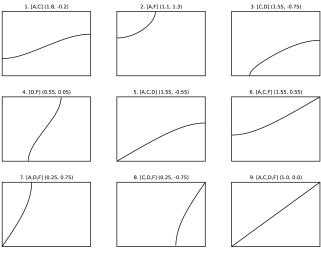
Figure 2: The family of possible curves of $\tensor*[^{O_{1}}_{2}]{S}{}$ within the patch $[0,\pi]\times[0,\pi]$ .

Finally note that a calculus analysis can provide the same result by showing that the slope of the curve within the patch is always positive.

II.4 Uniqueness of Solutions

Having obtained decent understanding of the single-sample problem and its characterizing solution curves we note that, in the absence of noise, insight into multi-sample problem can be gained by considering superpositions of the curves in the $(\theta_{1},\theta_{2})$ plane for each of the samples. We have seen that each $\tensor*[_{2}]{S}{}$ is symmetric about one of the $\tensor*[_{1}]{S}{}$ points. Due to this it becomes relevant to pose the question of existence of samples that have unequal data, equal $\tensor*[_{1}]{S}{}$ grids, but different $\tensor*[_{2}]{S}{}$ curves. When such samples intersect within one of the four sectors of a patch around a maximum, they necessarily intersect within all others creating three false minima for each true one. If additionally the intersection point can be quite arbitrary, the distances between the so obtained minima would be arbitrarily small and this would make the problem ill-posed. We proceed to find such two samples.

For any two samples $A$ and $B$, looking first at $\tensor*[_{1}]{S}{}$, we need $\sin(2\,\tensor[^{\scriptscriptstyle{A}}]{r}{{}_{i}})=0$ if and only if $\sin(2\,\tensor[^{\scriptscriptstyle{B}}]{r}{{}_{i}})=0$, which reduces to

$$\text{atan}[\frac{\tensor[^{\scriptscriptstyle{A}}]{w}{{}_{i{1}}}}{\tensor[^{\scriptscriptstyle{A}}]{w}{{}_{i{3}}}}]=\text{atan}[\frac{\tensor[^{\scriptscriptstyle{B}}]{w}{{}_{i{1}}}}{\tensor[^{\scriptscriptstyle{B}}]{w}{{}_{i{3}}}}],$$ (75)

Since we write atan when we really mean atan2, this is equivalent to

$$\left(\tensor[^{\scriptscriptstyle{A}}]{w}{{}_{i{1}}}\atop\tensor[^{\scriptscriptstyle{A}}]{w}{{}_{i{3}}}\right)=\lambda_{i}\left(\tensor[^{\scriptscriptstyle{B}}]{w}{{}_{i{1}}}\atop\tensor[^{\scriptscriptstyle{B}}]{w}{{}_{i{3}}}\right)+2k_{i}\pi,\quad\lambda_{i}>0.$$ (76)

This is then the condition for two samples to have identical $\tensor*[_{1}]{S}{}$ grids. Having obtained this, we turn to $\tensor*[_{2}]{S}{}$ looking for a family of curves passing through a specific point which we force to lie on the $x=y$ line to simplify finding an explicit example. Using the canonical form (74) we have at the common point $(t,t)$ that

$$\cos(t) =u\cos(t)+v,$$

$$\cos(t) =\frac{v}{1-u}.$$

Since the point is common to all curves its cosine must be equal in all of them so we have for two samples $A$ and $B$ that

$$\frac{\tensor[^{\scriptscriptstyle{A}}]{v}{}}{1-\tensor[^{\scriptscriptstyle{A}}]{u}{}} =\frac{\tensor[^{\scriptscriptstyle{B}}]{v}{}}{1-\tensor[^{\scriptscriptstyle{B}}]{u}{}}.$$

$$\tensor[^{\scriptscriptstyle{B}}]{u}{} =1-\tensor[^{\scriptscriptstyle{B}}]{v}{}\left[\frac{1+\tensor[^{\scriptscriptstyle{A}}]{u}{}}{\tensor[^{\scriptscriptstyle{A}}]{v}{}}\right].$$ (77)

Going back to the original form (68) and baking in the condition (76) (while dropping the $2\pi$ period since we are working within one patch) we have the two relations:

$$\tensor[^{\scriptscriptstyle{A}}]{v}{} =-1+\left(\frac{{\lambda_{2}}^{2}}{{\lambda_{1}}^{2}}\right)\frac{\tensor[^{\scriptscriptstyle{B}}]{s}{{}_{2}}}{\tensor[^{\scriptscriptstyle{B}}]{s}{{}_{1}}}-\frac{\tensor[^{\scriptscriptstyle{A}}]{\beta}{}}{({\lambda_{1}}^{2})\tensor[^{\scriptscriptstyle{B}}]{s}{{}_{1}}},$$

$$\tensor[^{\scriptscriptstyle{A}}]{u}{} =\left(\frac{{\lambda_{2}}^{2}}{{\lambda_{1}}^{2}}\right)\frac{\tensor[^{\scriptscriptstyle{B}}]{s}{{}_{2}}}{\tensor[^{\scriptscriptstyle{B}}]{s}{{}_{1}}}.$$

By (77) we then require the follwing relation between the samples:

$$\frac{\tensor[^{\scriptscriptstyle{B}}]{s}{{}_{2}}}{\tensor[^{\scriptscriptstyle{B}}]{s}{{}_{1}}}=1-\left[\frac{-1+\frac{\tensor[^{\scriptscriptstyle{B}}]{s}{{}_{2}}}{\tensor[^{\scriptscriptstyle{B}}]{s}{{}_{1}}}-\frac{\tensor[^{\scriptscriptstyle{B}}]{\beta}{}}{{\tensor[^{\scriptscriptstyle{B}}]{s}{{}_{1}}}}}{-1+\left(\frac{{\lambda_{2}}^{2}}{{\lambda_{1}}^{2}}\right)\frac{\tensor[^{\scriptscriptstyle{B}}]{s}{{}_{2}}}{\tensor[^{\scriptscriptstyle{B}}]{s}{{}_{1}}}-\frac{\tensor[^{\scriptscriptstyle{A}}]{\beta}{}}{({\lambda_{1}}^{2})\tensor[^{\scriptscriptstyle{B}}]{s}{{}_{1}}}}\right]\left[1+\left(\frac{{\lambda_{2}}^{2}}{{\lambda_{1}}^{2}}\right)\frac{\tensor[^{\scriptscriptstyle{B}}]{s}{{}_{2}}}{\tensor[^{\scriptscriptstyle{B}}]{s}{{}_{1}}}\right]$$ (78)

We denote

$$Q =\frac{\tensor[^{\scriptscriptstyle{B}}]{s}{{}_{2}}}{\tensor[^{\scriptscriptstyle{B}}]{s}{{}_{1}}},$$

$$R =\frac{{\lambda_{2}}^{2}}{{\lambda_{1}}^{2}},$$

and tentatively set

$$R=\frac{1}{Q}$$

which simplifies (78) to

$$R=1-2\left[R-1-\frac{\tensor[^{\scriptscriptstyle{B}}]{\beta}{}}{\tensor[^{\scriptscriptstyle{B}}]{s}{{}_{1}}}\right]\left[\frac{{(\lambda_{1}}^{2})\tensor[^{\scriptscriptstyle{B}}]{s}{{}_{1}}}{-\tensor[^{\scriptscriptstyle{A}}]{\beta}{}}\right]$$

Again tentatively setting

$$R=2$$

we obtain

$$\frac{{(\lambda_{1}}^{2})\tensor[^{\scriptscriptstyle{B}}]{s}{{}_{1}}}{-\tensor[^{\scriptscriptstyle{A}}]{\beta}{}} =2\left[1-\frac{\tensor[^{\scriptscriptstyle{B}}]{\beta}{}}{\tensor[^{\scriptscriptstyle{B}}]{s}{{}_{1}}}\right],$$

$$\tensor[^{\scriptscriptstyle{B}}]{\beta}{} =\tensor[^{\scriptscriptstyle{B}}]{s}{{}_{1}}-\frac{1}{2{\lambda_{1}}^{2}}\tensor[^{\scriptscriptstyle{A}}]{\beta}{}.$$

To finally obtain our example we set

$$\tensor[^{\scriptscriptstyle{B}}]{s}{{}_{1}} =4,$$

$${\lambda_{1}}^{2} =4,$$

$$\tensor[^{\scriptscriptstyle{A}}]{\beta}{} =4,$$

$${\lambda_{2}}^{2} =2,$$

This determines the two samples almost completely and by inspection we set

$$\tensor[^{\scriptscriptstyle{A}}]{w}{{}_{22}}=\tensor[^{\scriptscriptstyle{B}}]{w}{{}_{22}}=0,$$

to make the samples valid viz. satisfy (67). The samples are then

$$\tensor[^{\scriptscriptstyle{A}}]{w}{{}_{1}},\tensor[^{\scriptscriptstyle{A}}]{w}{{}_{2}} =(\sqrt{12},\sqrt{2},2),\,(\sqrt{2},0,\sqrt{14}),$$

$$\tensor[^{\scriptscriptstyle{B}}]{w}{{}_{1}},\tensor[^{\scriptscriptstyle{B}}]{w}{{}_{2}} =(\sqrt{3},\sqrt{\frac{7}{4}},1),\,(1,0,\sqrt{7}),$$

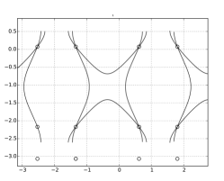
Figure 3: Two $\tensor*[_{2}]{S}{}$ curves intersecting at an arbitrarily chosen point. The minimum distance between the intersection points is less than $\frac{\pi}{3}$.The minima generated by running a non-linear least squares algorithm are shown using circles.

and the ensuing skinned cat figure (3) confirms the result.

Despite the barbarism of the attempt, we easily found our example. This indicates that a continuum of such curves almost certainly exists but we leave a proof of this as subject for further work. Thence, we have shown that the problem is from the point of view of unique solutions, ill-posed or more exactly, only conditionally well-posed.

III Appendix

III.1 Objective Function Intuition

Very few sentences are used in (Seel, Schauer, and Raisch 2012) to explain the derivation of the objective function. We here attempt an explanation with the following intuitive perspective.

Consider a canonical hinge setup. It naturally leads to conceptually thinking of the whole three-dimensional space as the union of two. The ‘hinge plane’ that is orthogonal to the hinge axis and in which the constrained bodies canonically lie, and it’s complement. The part of the angular velocities that determine the planar rotation within the hinge plane is given by projecting them onto the hinge axis. This exhausts the hinge’s single degree of freedom. The projection rests (also called rejections) must therefore be equal. Another way to think about this is that any difference in the rejections would ‘break’ the plane for the two canonical bodies would rotate such that they would not anymore lie in a common plane. By known vector projection and rejection formulas, with $a$ being the unit hinge axis, $\theta$ the hinge angle and $w_{i}$ being the angular velocities, we have:

$$\begin{split}w_{i}=\underbrace{(w_{i}\cdot a)a}_{\tensor[_{\parallel}]{w}{{}_{i}}}+\underbrace{a\times(w_{i}\times a)}_{\tensor[_{\perp}]{w}{{}_{i}}}.\\ \tensor[_{\parallel}]{w}{{}_{2}}-\tensor[_{\parallel}]{w}{{}_{1}}=\dot{\theta}a.\\ \tensor[_{\perp}]{w}{{}_{2}}-\tensor[_{\perp}]{w}{{}_{1}}=0.\end{split}$$

All of this holding in any space, our objective function simply expresses the equality of rejections in two unknown spaces. Since the spaces are unknown, the magnitude of both vectors is taken and the spaces that make the equality hold determine the sought for transformations.

III.2 Expressions Generated by SymPy

$$\begin{split}\frac{\partial O_{1}}{\partial\theta_{1}}&=(2(w_{11}\sin(\theta_{1})-w_{13}\cos(\theta_{1}))(2w_{11}\cos(\theta_{1})\\ &\quad+2w_{13}\sin(\theta_{1}))(w_{12}^{2}-w_{22}^{2}+(w_{11}\sin(\theta_{1})\\ &\quad-w_{13}\cos(\theta_{1}))^{2}-(w_{21}\sin(\theta_{2})-w_{23}\cos(th2))^{2}))\\ \frac{\partial^{2}O_{1}}{\partial\theta_{1}^{2}}&=(2(-2w_{11}\sin(\theta_{1})+2w_{13}\cos(\theta_{1}))(w_{11}\sin(\theta_{1})\\ &\quad-w_{13}\cos(\theta_{1}))(w_{12}^{2}-w_{22}^{2}+(w_{11}\sin(\theta_{1})\\ &\quad-w_{13}\cos(\theta_{1}))^{2}-(w_{21}\sin(th2)-w_{23}\cos(th2)\\ &\quad)^{2})+2(w_{11}\sin(\theta_{1})-w_{13}\cos(\theta_{1}))^{2}(2w_{11}\cos(\theta_{1})\\ &\quad+2w_{13}\sin(\theta_{1}))^{2}+2(w_{11}\cos(\theta_{1})+w_{13}\sin(\theta_{1})\\ &\quad)(2w_{11}\cos(\theta_{1})+2w_{13}\sin(\theta_{1}))(w_{12}^{2}-w_{22}^{2}+(w_{11}\sin(\theta_{1})\\ &\quad-w_{13}\cos(\theta_{1}))^{2}-(w_{21}\sin(th2)-w_{23}\cos(th2))^{2}))\\ |\text{Hess }{O_{1}}|&=(-4(w_{11}\sin(\theta_{1})-w_{13}\cos(\theta_{1}))^{2}(2w_{11}\cos(\theta_{1})\\ &\quad+2w_{13}\sin(\theta_{1}))^{2}(w_{21}\sin(\theta_{2})-w_{23}\cos(\theta_{2})\\ &\quad)^{2}(2w_{21}\cos(\theta_{2})+2w_{23}\sin(\theta_{2}))^{2}+(2(-2w_{11}\sin(\theta_{1})\\ &\quad+2w_{13}\cos(\theta_{1}))(w_{11}\sin(\theta_{1})-w_{13}\cos(\theta_{1})\\ &\quad)(w_{12}^{2}-w_{22}^{2}+(w_{11}\sin(\theta_{1})-w_{13}\cos(\theta_{1})\\ &\quad)^{2}-(w_{21}\sin(\theta_{2})-w_{23}\cos(\theta_{2}))^{2})+2(w_{11}\sin(\theta_{1})\\ &\quad-w_{13}\cos(\theta_{1}))^{2}(2w_{11}\cos(\theta_{1})+2w_{13}\sin(\theta_{1})\\ &\quad)^{2}+2(w_{11}\cos(\theta_{1})+w_{13}\sin(\theta_{1}))(2w_{11}\cos(\theta_{1})\\ &\quad+2w_{13}\sin(\theta_{1}))(w_{12}^{2}-w_{22}^{2}+(w_{11}\sin(\theta_{1})\\ &\quad-w_{13}\cos(\theta_{1}))^{2}-(w_{21}\sin(\theta_{2})-w_{23}\cos(\theta_{2})\\ &\quad)^{2}))(-2(-2w_{21}\sin(\theta_{2})+2w_{23}\cos(\theta_{2})\\ &\quad)(w_{21}\sin(\theta_{2})-w_{23}\cos(\theta_{2}))(w_{12}^{2}-w_{22}^{2}+(w_{11}\sin(\theta_{1})\\ &\quad-w_{13}\cos(\theta_{1}))^{2}-(w_{21}\sin(\theta_{2})-w_{23}\cos(\theta_{2})\\ &\quad)^{2})+2(w_{21}\sin(\theta_{2})-w_{23}\cos(\theta_{2}))^{2}(2w_{21}\cos(\theta_{2})\\ &\quad+2w_{23}\sin(\theta_{2}))^{2}-2(w_{21}\cos(\theta_{2})+w_{23}\sin(\theta_{2})\\ &\quad)(2w_{21}\cos(\theta_{2})+2w_{23}\sin(\theta_{2}))(w_{12}^{2}-w_{22}^{2}+(w_{11}\sin(\theta_{1})\\ &\quad-w_{13}\cos(\theta_{1}))^{2}-(w_{21}\sin(\theta_{2})-w_{23}\cos(\theta_{2}))^{2})))\end{split}$$

References

Seel, Thomas, Thomas Schauer, and Jörg Raisch. 2012. “Joint Axis and Position Estimation from Inertial Measurement Data by Exploiting Kinematic Constraints.” In Control Applications (CCA), 2012 IEEE International Conference on, 45–49. IEEE.

SymPy Development Team. 2014. SymPy: Python Library for Symbolic Mathematics. http://www.sympy.org.