Normalizer
of the Chevalley group of type ${\mathrm{E}}_{7}$

Abstract.

We consider the simply connected Chevalley group $G(\mathrm{E}_{7},R)$ of type $\mathrm{E}_{7}$ in the 56-dimensional representation. The main objective of the paper is to prove that the following four groups coincide: the normalizer of the elementary Chevalley group $E(\mathrm{E}_{7},R)$, the normalizer of the Chevalley group $G(\mathrm{E}_{7},R)$ itself, the transporter of $E(\mathrm{E}_{7},R)$ into $G(\mathrm{E}_{7},R)$, and the extended Chevalley group $\overline{G}(\mathrm{E}_{7},R)$. This holds over an arbitrary commutative ring $R$, with all normalizers and transporters being calculated in $\mathrm{GL}(56,R)$. Moreover, we characterize $\overline{G}(\mathrm{E}_{7},R)$ as the stabilizer of a system of quadrics. This last result is classically known over algebraically closed fields, here we prove that the corresponding group scheme is smooth over $\mathbb{Z}$, which implies that it holds over arbitrary commutative rings. These results are one of the key steps in our subsequent paper, dedicated to the overgroups of exceptional groups in minimal representations.

The most natural way to study general orthogonal group, is to represent it as the stabilizer of a quadric. In the present paper, we establish a similar geometric characterization of the normalizer of the simply connected Chevalley group $G_{\operatorname{sc}}(\operatorname{E}_{7},R)$ as the stabilizer of the intersection of 133 quadrics in a 56-dimensional space, and prove that the above normalizer coincides with the normalizer of the elementary Chevalley group $E_{\operatorname{sc}}(\operatorname{E}_{7},R)$.

The present work is a direct sequel of our papers [43, 24], where a similar exercise was carried through for the groups of types $\operatorname{E}_{6}$ and $\operatorname{F}_{4}$.

1. Introduction

In the paper [22] (see also [24, 23]) the second author has started to carry over the results by the first author and Victor Petrov [46, 47, 29] on overgroups of classical groups in vector representations, to the exceptional groups $E(\operatorname{E}_{6},R)$ and $E(\operatorname{E}_{7},R)$, in minimal representations. From the very start, it became apparent, that one the key steps necessary to carry through a reduction proof in the spirit of the cited papers, would be an explicit calculation of the normalizer of the above groups in the corresponding general linear group, $\operatorname{GL}(27,R)$ or $\operatorname{GL}(56,R)$, respectively.

In our previous paper [43] we have completely solved this problem for the group $E(\operatorname{E}_{6},R)$, whereas in [24] this problem is solved for the group $E(\operatorname{F}_{4},R)$. In the present paper, we consider in the same spirit the group of type $\operatorname{E}_{7}$.

More precisely, in §4 we explicitly construct an ideal $I$ in the ring of integer polynomials ${\mathbb{Z}}[x_{1},\ldots,x_{56}]$, generated by 133 quadratic forms $f_{1},\ldots,f_{133}$, which has the following property. Denote by $\operatorname{Fix}_{R}(I)$ the set of $R$-linear transformations, preserving the ideal $I$, see §4 for the precise definitions.

The first main objective of the present paper, is to prove the following result. Here, $G_{I}$ denotes the affine group scheme such that $G_{I}(R)=\operatorname{Fix}_{R}(I)$.

Theorem 1.

There is an isomorphism $G_{I}\cong\overline{G}_{\operatorname{sc}}(\operatorname{E}_{7},-)$ of affine groups schemes over ${\mathbb{Z}}$.

This result can be viewed as an explicit description of the extended simply connected Chevalley–Demazure group scheme $\overline{G}_{\operatorname{sc}}(\Phi,-)$ of type $\Phi=\operatorname{E}_{7}$, by equations. This scheme was constructed in [3], see also [34, 35, 40] and §2 below. For $\Phi=\operatorname{E}_{7}$ the most straightforward way to visualize the scheme $\overline{G}_{\operatorname{sc}}(\Phi,-)$ is to view it as the Levi factor of the parabolic subscheme of type $P_{8}$ in $G_{\operatorname{sc}}(\operatorname{E}_{8},-)$, where $G_{\operatorname{sc}}(\Phi,-)$ — is the usual simply connected Chevalley–Demazure groups scheme of type $\Phi$. We refer the reader to [28] as for the scheme-theoretic definition of parabolic subgroups and their Levi factors, see also [40] for the above identification itself.

Our results are intimately related to the description of $G_{\operatorname{sc}}(\operatorname{E}_{7},R)$ as the stabilizer of a system of four-linear forms on $V=V(\varpi_{7})$. Namely, in [25] we gave a new construction of a four-linear form $f\colon V\times V\times V\times V\to R$ and a symplectic form $h\colon V\times V\to R$, invariant under the action of the group $G_{\operatorname{sc}}(\operatorname{E}_{7},R)$. We reproduce the construction of the form $f$ in §3. The bulk of our system of quadratic forms consists of the second partial derivatives of the [regular part of] the form $f$.

It turns out that $G_{\operatorname{sc}}(\operatorname{E}_{7},R)$ is precisely the group of linear transformations preserving both $f$ and $h$:

$$G_{(f,h)}(R)=\{ g\in\operatorname{GL}(56,R)\mid f(gu,gv,gw,gz)=f(u,v,w,z),$$

$$h(gu,gv)=h(u,v)\text{ for all }u,v,w,z\in V\}.$$

It is only marginally more complicated to describe the extended group $\overline{G}_{\operatorname{sc}}(\operatorname{E}_{7},R)$ in terms of the forms $f$ and $h$. Namely, let

$$\overline{G}_{(f,h)}(R) =\{g\in\operatorname{GL}(56,R)\mid\text{there exist $\varepsilon,\varepsilon^{\prime}\in R^{*}$, $c_{2},c_{3},c_{4}\in R$}$$

$$\qquad\text{such that }f(gu,gv,gw,gz)=\varepsilon f(u,v,w,z)$$

$$\qquad\qquad+c_{2}h(u,v)h(w,z)+c_{3}h(u,w)h(v,z)+c_{4}h(u,z)h(v,w)$$

$$\qquad\text{and }h(gu,gv)=\varepsilon^{\prime}h(u,v)\text{ for all }u,v,w,z\in V\}.$$

Theorem 2.

There are isomorphisms $G_{(f,h)}\cong G_{\operatorname{sc}}(\operatorname{E}_{7},-)$, $\overline{G}_{(f,h)}\cong\overline{G}_{\operatorname{sc}}(\operatorname{E}_{7},-)$ of affine groups schemes over ${\mathbb{Z}}$.

This theorem readily implies that the above definition of the extended group $\overline{G}_{\operatorname{sc}}(\operatorname{E}_{7},R)$ can be simplified as follows. Namely, Lemma 10 asserts that

$$\overline{G}_{(f,h)}(R) =\{g\in\operatorname{GL}(56,R)\mid\text{there exists an $\varepsilon\in R^{*}$ such that}$$

$$\qquad f(gu,gv,gw,gz)=\varepsilon f(u,v,w,z)$$

$$\qquad\text{and }h(gu,gv)=\varepsilon^{2}h(u,v)\text{ for all }u,v,w,z\in V\}.$$

Now, let $E,F$ be two subgroups of a group $G$. Recall that the transporter of the subgroup $E$ to the subgroup $F$ is the set

$$\operatorname{Tran}_{G}(E,F)=\{g\in G\mid E^{g}\leqslant F\}.$$

Actually, we mostly use this notation in the case where $E\leqslant F$, and then

$$\operatorname{Tran}_{G}(E,F)=\{g\in G\mid[g,E]\leqslant F\}.$$

In the sequel, we only work with the simply connected groups and omit the subscript in the notation $G_{\operatorname{sc}}(\Phi,R)$. By $E(\Phi,R)\leqslant G(\Phi,R)$ we denote the elementary Chevalley group. Now we are all set to state the main result of the present paper. Observe, that all normalizers and transporters here are taken in the general linear group $\operatorname{GL}(56,R)$.

Theorem 3.

Let $R$ be an arbitrary commutative ring. Then

$$N(E(\operatorname{E}_{7},R))=N(G(\operatorname{E}_{7},R))=\operatorname{Tran}(E(\operatorname{E}_{7},R),G(\operatorname{E}_{7},R))=G_{I}(R).$$

The interrelation of Theorems 1 and 3 and the general scheme of their proof are exactly the same, as in our previous paper[43], and some familiarity with [43] (at least with the introduction and §5) would be extremely useful to facilitate understanding the proofs in the present paper.

Observe, that after the publication of [43] its subject matter became unexpectedly pertinent. Namely, recently Elena Bunina reconsidered one of the central classical problems of the whole theory, description of [abstract] automorphisms of Chevalley groups, without any such simplifying assumptions as $R$ being Noetherian, or $2$ being invertible in $R$. For local rings she almost succeeded in proving that all automorphisms of the group $E(\Phi,R)$ are standard, see [7], etc. Namely, she established that an arbitrary automorphism of the adjoint elementary Chevalley group is the product of ring, inner and graph automorphisms. There is a catch, though, that with her approach the inner automorphisms are taken not in the adjoint Chevalley group $G_{\operatorname{ad}}(\Phi,R)$ itself, but rather in the corresponding general linear group ${\mathrm{GL}}(n,R)$. In this context, the fact that the abstract and algebraic normalizers coincide, means precisely that all such conjugations are genuine inner automorphisms.

This means that modulo the results of [7] an analogue of the results of [43] and the present paper, for adjoint representations would then imply that all automorphisms of Chevalley groups of types $\operatorname{E}_{l}$ over local rings — and thus also arbitrary commutative rings — are standard in the usual sense. We are convinced that our results on the equations in adjoint representations [26, 27] allow to obtain the requisite results for the adjoint case. In cooperation with Elena Bunina, we hope to work out the details shortly.

The paper is organized as follows. In §2 we recall the basic notation pertaining to the extended Chevalley group of type $\operatorname{E}_{7}$. In §3 we discuss the invariant four-linear forms, and in §4 we construct an invariant system of quadrics, which in this case is significantly trickier than in the case of $\operatorname{E}_{6}$. In §5 we prove that this system of quadrics is indeed invariant. The technical core of the paper are §§6–10, which are directly devoted to the proof of Theorems 1, 2 and 3. Due to the limited space, we do not explicitly list the resulting equations here, this will be done in a subsequent publication.

2. Extended Chevalley group of type $\operatorname{E}_{7}$

We refer the reader to [43] as for the general context of the present paper, and further references. In the papers [28, 32, 36, 37, 48] one can find many further details pertaining to Chevalley groups over rings, and many further related references.

Nevertheless, to fix the requisite notation, for reader’s convenience below we reproduce with minor modifications §1 of [43].

Let $\Phi$ be a reduced irreducible root system of rank $l$ (in the main body of the paper we assume that $\Phi=\operatorname{E}_{7}$), and $P$ be a lattice intermediate between the root lattice $Q(\Phi)$ and the weight lattice $P(\Phi)$. We fix and order on $\Phi$ and denote by $\Pi=\{\alpha_{1},\ldots,\alpha_{l}\}$, $\Phi^{+}$ and $\Phi^{-}$ the corresponding sets of fundamental, positive, and negative roots. Our numbering of the fundamental roots follows [5]. By $\delta$ we denote the maximal root of the system $\Phi$ with respect to this order. For instance, for $\Phi=\operatorname{E}_{7}$ we have $\delta=\vbox{\vbox{\vfill\hbox{$234321$} \nointerlineskip\vskip 3.0pt\hbox{$\phantom{2}\phantom{3}2$\hfil}\vfill}}$. Denote by $P(\Phi)_{++}$ the set of dominant weights with respect to this order. Recall that it consists of all nonnegative integral linear combinations of the fundamental weights ${\varpi}_{1},\ldots,{\varpi}_{l}$, for this order. Finally, $W=W(\Phi)$ denotes the Weyl group of the root system $\Phi$.

Further, let $R$ be a commutative ring with 1. It is classically known that, starting with this data, one can construct the Chevalley group $G_{P}(\Phi,R)$, which is the group of $R$-points of an affine group scheme $G_{P}(\Phi,{-})$, known as the Chevalley–Demazure scheme. For the problems we consider, it suffices to limit ourselves with the simply connected (alias, universal) groups, for which $P=P(\Phi)$. For the simply connected groups we usually omit any reference to the lattice $P$ and simply write $G(\Phi,R)$ or, when we wish to stress that the group in question is simply connected, $G_{\operatorname{sc}}(\Phi,R)$. The adjoint group, for which $P=Q(\Phi)$, is denoted by $G_{\operatorname{ad}}(\Phi,R)$.

Fix a split maximal torus $T(\Phi,R)$ in $G(\Phi,R)$ and a parametrization of the unipotent root subgroups $X_{\alpha}$, $\alpha\in\Phi$, elementary with respect to this torus. Let $x_{\alpha}(\xi)$ be the elementary unipotent element corresponding to $\alpha\in\Phi$ and $\xi\in R$ in this parametrization. The group $X_{\alpha}=\{x_{\alpha}(\xi),\xi\in R\}$ is called an (elementary) root subgroup, and the group $E(\Phi,R)=\langle X_{\alpha},\alpha\in\Phi\rangle$ generated by all elementary root subgroups is called the (absolute) elementary subgroup of the Chevalley group $G(\Phi,R)$.

As a matter of fact, apart from the usual Chevalley group, we also consider the corresponding extended Chevalley group $\overline{G}(\Phi,R)$, which plays the same role with respect to $G(\Phi,R)$ as the general linear group $\operatorname{GL}(n,R)$ plays with respect to the special linear group $\operatorname{SL}(n,R)$. Adjoint extended groups were constructed in the original paper by Chevalley [8]. It is somewhat harder to construct simply connected extended groups because, unlike the adjoint case, here one must increase the dimension of the maximal torus. A unified elementary construction was only proposed by Berman and Moody in [3]. However, for the case of $\overline{G}_{\operatorname{sc}}(\operatorname{E}_{7},R)$ that we consider in the present paper, this group can be naturally viewed as a subgroup of the usual Chevalley group $G_{\operatorname{sc}}(\operatorname{E}_{8},R)$, viz.

$$\overline{G}_{\operatorname{sc}}(\operatorname{E}_{7},R)=G_{\operatorname{sc}}(\operatorname{E}_{7},R)\cdot T_{\operatorname{sc}}(\operatorname{E}_{8},R).$$

In the majority of the existing constructions, the Chevalley group $G(\Phi,R)$ arises together with an action on the Weyl module $V=V(\omega)$, for some dominant weight $\omega$. Denote by $\Lambda=\Lambda(\omega)$ the multiset of weights of the module $V=V(\omega)$ with multiplicities. In the present paper we consider the group $G(\operatorname{E}_{7},R)$ in the minimal representation with the highest weight $\varpi_{7}$. This is a microweight representation, in particular the multiplicities of all weights are equal to 1. Fix an admissible base $v^{\lambda}$, $\lambda\in\Lambda$, of the module $V$. We conceive a vector $a\in V$, $a=\sum v^{\lambda}a_{\lambda}$, as a coordinate column $a=(a_{\lambda})$, $\lambda\in\Lambda$.

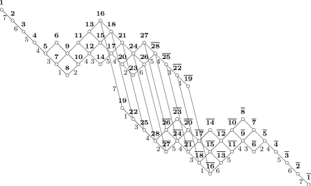
Figure 1. Weight diagram $(\operatorname{E}_{7},\varpi_{7})$: natural numbering.

In Figure 1 we reproduce the weight diagram of the representation $(\operatorname{E}_{7},\varpi_{7})$, together with the natural numbering of weights, used in the sequel. In this numbering the weights are listed according to the order determined by the fundamental root system $\Pi$. On the picture, the highest weight is the left-most one. The weight diagram of the representation $(\operatorname{E}_{7},\varpi_{7})$ is symmetric, and this symmetry is reflected in the numbering, the weights are numbered as $1,2,\dots,28,-28,\dots,2,1$. Often, to save space we write $\overline{n}$ instead of $-n$. We refer the reader to [44] for lists of weight in the Dynkin form, and in the hyperbolic form, as well as other common numberings.

Recall, that in the weight diagram two weights are joined by an edge if their difference is a fundamental root. The weight graph is constructed similarly, only that now two weights are joined by an edge provided their difference is a positive root. In the sequel we denote by $d(\lambda,\mu)$ the distance between two weights $\lambda$ and $\mu$ in the weight graph. In other words, $d(\lambda,\mu)=0$ if $\lambda=\mu$; $d(\lambda,\mu)=1$ if $\lambda-\mu\in\Phi$; $d(\lambda,\mu)=2$ if $\lambda\neq\mu$, $\lambda-\mu\not\in\Phi$, $\lambda-\mu$ is the sum of two roots of $\Phi$; and finally, $d(\lambda,\mu)=3$ otherwise.

The above realization of the representation $(\operatorname{E}_{7},\varpi_{7})$ as an internal Chevalley module inside the Chevalley group of type $\operatorname{E}_{8}$ provides a natural identification of the set of weights $\Lambda$ with the set of roots of the root system $\operatorname{E}_{8}$, in whose expansion with respect to the fundamental roots the root $\alpha_{8}$ occurs with the coefficient $1$. Obviously, the roots of the root system $\operatorname{E}_{7}$ itself are identified with those roots of $\operatorname{E}_{8}$ in whose expansion $\alpha_{8}$ occurs with the coefficient 0. There is a unique root of $\operatorname{E}_{8}$, in whose expansion $\alpha_{8}$ occurs with the coefficient $2$: it is the maximal root $\delta=\vbox{\vbox{\vfill\hbox{$2465432$} \nointerlineskip\vskip 3.0pt\hbox{$\phantom{2}\phantom{4}3$\hfil}\vfill}}$. In the sequel we always view both the roots of $\operatorname{E}_{7}$ and the wights of our representation as the roots of $\operatorname{E}_{8}$. We denote by $(\cdot,\cdot)$ the natural inner product defined on the linear span of $\operatorname{E}_{8}$. It is convenient to normalize it in such a way that all roots have length $1$. Then for any $\alpha,\beta\in\operatorname{E}_{8}$ the inner product $(\alpha,\beta)$ can take values $0$, $\pm 1/2$ or $\pm 1$. With these conventions, the distance $d(\lambda,\mu)$ between the weights $\lambda,\mu\in\Lambda$ equals

• $0$ if $(\lambda,\mu)=1$;

• $1$ if $(\lambda,\mu)=1/2$;

• $2$ if $(\lambda,\mu)=0$;

• $3$ if $(\lambda,\mu)=-1/2$ (and then $\lambda+\mu=\delta$).

Thus, for any weight $\lambda\in\Lambda$ there exists a unique weight at distance $3$; this is the weight $\delta-\lambda$, which will be denoted by $\overline{\lambda}$.

In [33, 30, 36, 37, 39] one can find many further details as to how to recover, from this diagram alone, the action of root unipotents $x_{\alpha}(\xi)$, $w_{\alpha}(\varepsilon)$, $h_{\alpha}(\varepsilon)$, the signs of structure constants, the shape and signs of equations, etc. These and other such similar items are tabulated in [44]. Formally, an explicit knowledge of these things is not necessary to understand the proofs produced in the present paper. However, in reality all calculations in §3, 4, 7–9, were performed with the heavy use of weight diagrams, and could hardly be possible without them.

Over a field, and in general over a semilocal ring, the extended Chevalley group $\overline{G}(\operatorname{E}_{7},R)$ is generated by the usual Chevalley group $G(\operatorname{E}_{7},R)$ and the weight elements $h_{\varpi_{7}}(\eta)$, $\eta\in R^{*}$. In the natural numbering of weight the element $h_{\varpi_{7}}(\eta^{-1})$ acts on the module $V(\varpi_{7})$ as follows:

$$\operatorname{diag}(\eta^{-1},1,1,1,1,1,1,1,1,1,1,1,1,1,1,1,1,1,\eta,1,1,\eta,1,1,\eta,1,1,\eta,$$

$$\quad\qquad 1,\eta,\eta,1,\eta,\eta,1,\eta,\eta,1,\eta,\eta,\eta,\eta,\eta,\eta,\eta,\eta,\eta,\eta,\eta,\eta,\eta,\eta,\eta,\eta,\eta,\eta^{2}).$$

Here we assume that the weights are linearly ordered as follows: $1,\dots,28,\overline{28},\dots,\overline{1}$). Observe, that the exponent of $\eta$ increases by 1 each time we cross an edge marked $\alpha_{7}$.

3. The invariants of degree 4

In our paper [43] the simply connected Chevalley group of type $\operatorname{E}_{6}$ acting on the $27$-dimensional module $V=V({\varpi}_{1})$ was identified with the isometry group of a three-linear form $T\colon V\times V\times V\longrightarrow R$. There is a similar, but much more complicated description of the simply connected Chevalley group of type $\operatorname{E}_{7}$ acting on the $56$-dimensional module $V=V({\varpi}_{7})$. In this case, to determine the group one needs to invariants, one of degree 2, and another one of degree 4. First of all, the module $V$ is self-dual and carries a unimodular symplectic form $h$. Further, there exists a four-linear form $f:V\times V\times V\times V\longrightarrow R$ such that $G$ can be identified with the full isometry group of the pair $h$, $f$, in other words, with the group of all $g\in\operatorname{GL}(V)$ such that $h(gu,gv)=h(u,v)$ and $f(gu,gv,gw,gz)=f(u,v,w,z)$ for all $u,v,w,z\in V$. The similarities of this pair of forms define the extended Chevalley group $\overline{G}(\operatorname{E}_{7},R)$ (see Theorem 2).

It is obvious how to construct $h$. Construction of the fourth degree invariant is considerably more complicated, and classically one constructs not the four-linear form $f$, but rather the corresponding quartic. The fact that the group $G$ preserves a form of degree 4 in 56 variables, was first observed by E. Cartan, at least in characteristic 0, but his explicit construction of this form was flawed (probably, it was just a misprint). A very elegant construction of such an invariant over a field $K$ of characteristic distinct from 2 was given by H. Freudenthal. Namely, he identifies the module $V$ with the space $A(8,K)^{2}$, where $A(8,K)$ is the set of antisymmetric $8\times 8$ matrices, and considers the following symplectic inner product and form of degree 4:

$$h((a_{1},b_{1}),(a_{2},b_{2})) =\frac{1}{2}(\operatorname{tr}(a_{1}b_{2}^{t})-\operatorname{tr}(a_{2}b_{1}^{t})),$$

$$Q((a,b)) =\operatorname{pf}(a)+\operatorname{pf}(b)-\frac{1}{4}\operatorname{tr}((ab)^{2})+\frac{1}{16}\operatorname{tr}(ab)^{2}.$$

Now, for all characteristics distinct from 2, one can identify the isometry group of this pair with the simply-connected Chevalley group $G$ of type $\operatorname{E}_{7}$ over $K$ (see [2, 9]). The constructions of the above form in the papers by M. Aschbacher and B. Cooperstein is somewhat different. Actually, in [2] the form is constructed in terms of $\operatorname{A}_{6}$ (the gist of this construction is expressed by the partition $56=7+21+21+7$), whereas the construction in [9] is closer to Freudenthal’s original construction, and is phrased in terms of $\operatorname{A}_{7}$ (where $56=28+28$). The isometry group of the form $Q$ is generated by $G$ and a diagonal element of order 2 (see [9]). There are no serious complications in characteristic $p\geqslant 5$, whereas characteristic 3 requires some extra-care.

However, in characteristic 2 this approach is almost immediately blocked by serious obstacles. Obviously, the above construction fails. Apparently, in characteristic 2 there are whatsoever no non-trivial symmetric $G$-invariant four-linear forms on $V$, (see [2]). This is related to the fact that in characteristic 2 the four-linear form

$$f_{0}(u,v,x,y)=h(u,v)h(x,y)+h(u,x)h(v,y)+h(u,y)h(v,x),$$

obtained by the squaring of the symplectic form, becomes symmetric, which is not the case in characteristics $\geqslant 3$. Actually, in characteristic 2 M. Aschbacher [2] constructs a four-linear $G$-invariant form $F$, which is symmetric with respect to the even permutations.

There are other constructions of the form $Q$, most notably a construction by R. Brown [6], which works in characteristics $\neq 2,3$. Let $V$ be a space with a non-degenerate inner product. Then to define a three-linear form on $V$ is essentially the same as to define on $V$ an algebra structure. By the same token, to define a four-linear form on $V$ is essentially the same as to define on $V$ a ternary algebra structure. Indeed, there exists a remarkable ternary algebra of dimension 56, constructed in terms of the exceptional 27-dimensional Jordan algebra $\mathbb{J}$ (see [6, 12] and references there). This algebra consists of $2\times 2$ matrices over $\mathbb{J}$ with scalar diagonal entries, $56=1+27+27+1$.

The orbits of the group $G=G(\operatorname{E}_{7},K)$ on the 56-dimensional module are classified in [15] in the absolute case, in [20] for finite fields, and in [9] for arbitrary fields. Basically, these orbits are described in terms of the four-linear form. Again characteristics 2 and 3 require separate analysis, and to take care of all details one has to use the notion of 4-forms, introduced by M. Aschbacher (see [2, 9]). Essentially, a 4-form is a form of degree 4 together with all of its polarizations. For simplicity, assume that $\operatorname{char}K\neq 2,3$. Then a vector $u\in V$ is called singular, if $F(u,u,x,y)=0$ for all $x,y\in V$; brilliant, if $F(u,u,u,x)=0$ for all $x\in V$; and luminous if $F(u,u,u,u)=0$. Otherwise, i.e. if $F(u,u,u,u)\neq 0$, the vector $u$ is called dark. The orbits of the group $G$ on $V$ are as follows: 0, non-zero singular vectors, non-singular brilliant vectors, luminous vectors that are non brilliant, and, finally, one or several orbits of dark vectors, parametrized by $K^{*}/K^{*2}$ (these last orbits fuse to one orbit under the action of the extended Chevalley group $\overline{G}$ of type $\operatorname{E}_{7}$).

The feeling that $\operatorname{E}_{7}$ stands in the same relation to $\operatorname{E}_{6}$, as $\operatorname{E}_{6}$ itself stands to $\operatorname{D}_{5}$, suggests the following definition of the form of degree 4 on $V$. Take a base vector $v^{\lambda}$. Then the vectors $v^{\mu}$, $d(\lambda,\mu)=2$, generates a 27-dimensional module $U$, that supports the cubic form related to $\operatorname{E}_{6}$. Let us define tetrads as quadruples $(\lambda_{1},\lambda_{2},\lambda_{3},\lambda_{4})$ of pair-wise orthogonal weights. Let $\Theta$ and $\Theta_{0}$ be the sets of ordered and unordered tetrads, respectively. Clearly, $|\Theta|=56\cdot 27\cdot 10$, whereas $|\Theta_{0}|=|\Theta|/24=630$. Now, we can tentatively define the form $Q_{\operatorname{tent}}$ of degree 4 by setting $Q_{\operatorname{tent}}(x)=\sum\pm x_{\lambda_{1}}x_{\lambda_{2}}x_{\lambda_{3}}x_{\lambda_{4}}$, where the sum is taken over all $\{\lambda_{1},\lambda_{2},\lambda_{3},\lambda_{4}\}\in\Theta_{0}$, while the signs are determined by the condition that the resulting form is invariant under the action of the extended Weyl group $\widetilde{W}$. Here, one should be slightly more cautious then in the case of $\operatorname{E}_{6}$, since now, in addition to the two possible cases that occurred there, the following possibility occurs: $w_{\alpha}$ moves all 4 weights of a tetrad, two of them in positive and the other two in negative direction, in which case the signs does not change. Nevertheless, an expression of the sign in terms of $h(\lambda_{i},\mu_{i})$ still works. This is essentially the same, as to define the four-linear form $F_{\operatorname{tent}}$ by $F_{\operatorname{tent}}(v^{\lambda_{1}},v^{\lambda_{2}},v^{\lambda_{3}},v^{\lambda_{4}})=(-1)^{h(\lambda_{1},\lambda_{2},\lambda_{3},\lambda_{4})}$, for a tetrad $(\lambda_{1},\lambda_{2},\lambda_{3},\lambda_{4})\in\Theta$ and by $F_{\operatorname{tent}}(v^{\lambda_{1}},v^{\lambda_{2}},v^{\lambda_{3}},v^{\lambda_{4}})=0$ otherwise. By construction, this form is invariant under the action of $\widetilde{W}$, and we only have to verify that it is invariant under the action of the root subgroup $X_{\alpha}$, for some root $\alpha\in\Phi$. Unfortunately, this is not the case. Namely, for any tetrad $(\lambda_{1},\lambda_{2},\lambda_{3},\lambda_{4})$ and any elementary root unipotent $g=x_{\alpha}(\xi)$ the following formula holds

$$F_{\operatorname{tent}}(gv^{\lambda_{1}},gv^{\lambda_{2}},gv^{\lambda_{3}},gv^{\lambda_{4}})=F_{\operatorname{tent}}(v^{\lambda_{1}},v^{\lambda_{2}},v^{\lambda_{3}},v^{\lambda_{4}}).$$

As it happens, though, there exist quadruples of weights that are not tetrads, for which the right hand side equals 0, whereas the left hand side is distinct from 0. For instance, take the four weights $\lambda_{1},\lambda_{2},\lambda_{3},\lambda_{4}$ such that $\lambda_{1}+\alpha,\lambda_{2}+\alpha,\break\lambda_{3}+\alpha,\lambda_{4}-\alpha$ are weights, and together the 8 above weights form a cube (in other words, the corresponding weight diagrams is the tensor product of three copies $(\operatorname{A}_{1},{\varpi}_{1})$, see [9, 30]). Then one of the weights $\lambda_{1},\lambda_{2},\lambda_{3}$ will be adjacent with the other two, say, $d(\lambda_{1},\lambda_{2})=d(\lambda_{1},\lambda_{3})=1$, so that $F_{\operatorname{tent}}(v^{\lambda_{1}},v^{\lambda_{2}},v^{\lambda_{3}},v^{\lambda_{4}})=0$.

At the same time, decomposing the expression $F_{\operatorname{tent}}(gv^{\lambda_{1}},gv^{\lambda_{2}},gv^{\lambda_{3}},gv^{\lambda_{4}})$ by linearity, we get 8 summands, of which exactly one, namely $F_{\operatorname{tent}}(v^{\lambda_{1}+\alpha},v^{\lambda_{2}},v^{\lambda_{3}},v^{\lambda_{4}})$, corresponds to a tetrad, and equals $\pm 1$. Thus, the form $F_{\operatorname{tent}}$ is not preserved by the action of $X_{\alpha}$.

In itself, this is not yet critical, since one can hope to save the situation by throwing in another Weyl orbit of monomials. This is, however, exactly the point where real problems start. As a matter of fact, in the above counter-example throwing in another orbit of monomials will produce two non-zero extra summands, so that the resulting correction will be a multiple of 2. This means that one cannot define an invariant form of degree 4 by setting its values on the tetrads to be equal to $\pm 1$, one should start with $\pm 2$ instead. This is precisely where serious trouble starts. In characteristic $\neq 2$ the above construction is essentially correct, in the sense that it tells how the relevant part of an invariant form of degree 4 looks like, responsible for the reduction to $\operatorname{E}_{6}$. Let us fix a vector $v^{\lambda}$. Then $F(v^{\lambda},{-},{-},{-})$ consists of two parts: the form $F_{\operatorname{tent}}$, as defined above, and another part, introduced for the resulting form to be $G$-invariant. This second part has the form $F(v^{\lambda},v^{\lambda^{*}},{-},{-})$ and does not say anything beyond the fact that our group preserves the usual symplectic form.

In the works by Jacob Lurie [21] and the second author [25], these difficulties arising in characteristic 2 were sorted out in a systematic way, but the resulting four-linear forms are not anymore symmetric. Namely, let $\mathfrak{g}$ be the Lie algebra of type $\operatorname{E}_{8}$; recall that

$$\delta=\vbox{\vbox{\vfill\hbox{$2465432$} \nointerlineskip\vskip 3.0pt\hbox{$\phantom{2}\phantom{4}3$\hfil}\vfill}}$$

is the highest root of $\operatorname{E}_{8}$. The coefficient with which $\alpha_{8}$ occurs in the expansion of a root $\alpha\in\operatorname{E}_{8}$ with respect to the fundamental roots, is called the $\alpha_{8}$-height of $\alpha$ and can only take values $-2$, $-1$, $0$, $1$, $2$. This defines the following length 5 grading of the algebra $\mathfrak{g}$:

$$\mathfrak{g}=\mathfrak{g}_{-2}\oplus\mathfrak{g}_{-1}\oplus\mathfrak{g}_{0}\oplus\mathfrak{g}_{1}\oplus\mathfrak{g}_{2}.$$

The 56-dimensional space $\mathfrak{g}_{1}$ has a base consisting of the elementary root elements $e_{\alpha}$, where $\alpha$ runs over the roots of $\alpha_{8}$-height $1$, i.e. the weights of $V(\varpi_{7})$. Let $\lambda,\mu,\nu,\rho$ be four weights of $V(\varpi_{7})$. Clearly, the element

$$[[[[e_{-\delta},e_{\lambda}],e_{\mu}],e_{\nu}],e_{\rho}]$$

has $\alpha_{8}$-weight $2$, so that the resulting element is a multiple of $e_{\delta}$. Denote the corresponding scalar coefficient by $c(\lambda,\mu,\nu,\rho)$ and consider the four-linear form

$$f(u,v,w,z)=\sum_{\lambda,\mu,\nu,\rho\in\Lambda}c(\lambda,\mu,\nu,\rho)u_{\lambda}v_{\mu}w_{\nu}z_{\rho}.$$

Obviously, this form is invariant under the action of the group $G(\operatorname{E}_{7},R)$ on the module $V(\varpi_{7})$.

The orbit of the highest weight vector

It is well known that in any representation of the group $G$ the orbit $Gv^{+}$ of the highest weight vector $v^{+}$ is an intersection of quadrics [19]. Here, as a motivation for the next section, we explicitly describe the equations defining the orbit of $v^{+}$ for the microweight representation of $\operatorname{E}_{7}$. For the microweight representation of $\operatorname{E}_{6}$ this was done in [11]. Of course, for these cases the corresponding equations were found by H. Freudenthal and J. Tits more than 40 years ago (see also [44] and references there), but again we wish to show how to recover the equations directly from the weight diagram.

Let $\omega={\varpi}_{1}$ for $\operatorname{E}_{6}$ or $\omega={\varpi}_{7}$ for $\operatorname{E}_{7}$, the case of $(\Phi,\omega)=(\operatorname{E}_{6},{\varpi}_{6})$ is dual to the first case. We use the same interpretation of the modules as in § 1. In particular, $\Phi=\operatorname{E}_{l}$, $l=6,7$, $\Delta=E_{l+1}$, and $\Sigma=\Sigma_{l+1}(1)$. The group $G=G(\Phi,R)$ acts on $V=U_{l+1}(1)/U_{l+1}(2)\cong\prod X_{\alpha}$, $\alpha\in\Sigma$ by conjugation. Since we are only interested in the equations satisfied by the orbit $Gv^{+}$, we can assume that $R=K$ is an (algebraically closed) field.

In both cases one can take $v^{+}=v^{\rho}=x_{\rho}(1)$ as the highest weight vector, where

$$\rho=\vbox{\vbox{\vfill\hbox{$234321$} \nointerlineskip\vskip 3.0pt\hbox{$\phantom{2}\phantom{3}2$\hfil}\vfill}}\quad\text{or}\quad\rho=\vbox{\vbox{\vfill\hbox{$2465431$} \nointerlineskip\vskip 3.0pt\hbox{$\phantom{2}\phantom{4}3$\hfil}\vfill}}$$

is the maximal root of $\operatorname{E}_{7}$, or the unique submaximal root of $\operatorname{E}_{8}$, respectively. Recall that the vector $a=(a_{\alpha})\in V$ is now viewed as the product $x=\prod x_{\alpha}(a_{\alpha})\in\prod X_{\alpha}$, $\alpha\in\Sigma$. In the case of $\operatorname{E}_{7}$ this product is considered modulo $U_{8}(2)=X_{\rho+\alpha_{8}}$, the root subgroup corresponding to the maximal root of $\operatorname{E}_{8}$.

4. Construction of the system of quadrics

The first set of quadrics defining the highest weight orbit, consists of square equations; for large classes of representations, their construction and numerology were described by the first author in [41, 42]. Here, we recall some basic definitions of [41] in the context of the 56-dimensional representation of $(\operatorname{E}_{7},\varpi_{7})$.

The set of weights $\Omega\subseteq\Lambda$ is called a square if $|\Omega|\geqslant 4$ and for all $\lambda\in\Omega$ its difference $\lambda-\mu$ with all weights $\mu\in\Omega$, except exactly one, denoted by $\lambda^{*}$, is a root, whereas the difference $\lambda-\lambda^{*}$ is not a root (and thus $\lambda\perp\lambda^{*}$). A square maximal with respect to inclusion is called a maximal square. In [41] it is proven that for our representation each maximal square $\Omega$ consists of $12$ weights and the sum $\lambda+\lambda^{*}$ does not depend on the choice of $\lambda\in\Omega$. At that, a maximal square $\Omega$ is completely determined by this sum. Furthermore, in the case of a microweight representation of $\operatorname{E}_{7}$ maximal squares are in bijective correspondence with the roots of $\operatorname{E}_{7}$, namely, to a root $\alpha\in\operatorname{E}_{7}$ there corresponds the square

$$\Omega(\alpha)=\{\lambda\in\Lambda\mid\lambda-\alpha\in\Lambda\}.$$

Let, as above, $\Omega$ be some maximal square. Choose orthogonal weights $\rho,\rho^{*}\in\Omega$ and define the polynomial $f_{\rho,\rho^{*}}\in{\mathbb{Z}}[\{x_{\lambda}\}_{\lambda\in\Lambda}]$ by

$$f_{\rho,\rho^{*}}=x_{\rho}x_{\rho^{*}}-\sum N_{\rho,-\lambda}N_{\rho^{*},-\lambda^{*}}x_{\lambda}x_{\lambda^{*}},$$

where the sum is taken over all orthogonal pairs of weights $\{\lambda,\lambda^{*}\}$, except $\{\rho,\rho^{*}\}$ itself. The equation $f_{\rho,\rho^{*}}(v)=0$ on the components of a vector $v=(v_{\lambda})_{\lambda\in\Lambda}\in V$ was called in [41] a square equation, corresponding to the maximal square $\Omega$. In particular, this equation depends only on the square $\Omega$ itself, and not on the arbitrary choice of a pair $\rho,\rho^{*}$ of orthogonal weights: passing to another such pair, the polynomial $f_{\rho,\rho^{*}}$ is multiplied by $\pm 1$.

Fixing in each maximal square $\Omega$ one such pair of orthogonal weights gives us $126$ polynomials, corresponding (up to sign) to the $126$ maximal squares (or, what is the same, to the $126$ roots of $\operatorname{E}_{7}$).

Finally, for a root $\alpha\in\operatorname{E}_{7}$ we consider the polynomial $g_{\alpha}\in{\mathbb{Z}}[\{x_{\lambda}\}_{\lambda\in\Lambda}]$, defined by

$$g_{\alpha}=\sum_{\lambda\in\Omega(\alpha)}N_{\lambda,\overline{\lambda}}x_{\lambda}x_{\overline{\lambda}}.$$

Again, by definition these polynomials are in bijective correspondence with the roots of $\operatorname{E}_{7}$ (i.e. there are $126$ of them), but the following lemma asserts that it suffices to consider only $g_{\alpha}$ corresponding to $\alpha\in\Pi$.

Lemma 1.

The ideal in ${\mathbb{Z}}[\{x_{\lambda}\}_{\lambda\in\Lambda}]$, generated by the polynomials $\{g_{\alpha}\}$, $\alpha\in\operatorname{E}_{7}$, coincides with the ideal, generated by the polynomials $\{g_{\alpha}\}_{\alpha\in\Pi}$.

Proof.

Let $\alpha\in\operatorname{E}_{7}$. Observe, that $\Omega(\alpha)=\{\lambda\in\Lambda\mid\lambda-\alpha\in\Lambda\}=\{\lambda\in\Lambda\mid(\lambda,\alpha)=1/2\}$. If $\lambda\in\Omega(\alpha)$, then $(\overline{\lambda},-\alpha)=(\delta-\lambda,-\alpha)=(\lambda,\alpha)-(\delta,\alpha)=(\lambda,\alpha)$, since $\delta\perp\alpha$ for all $\alpha\in\operatorname{E}_{7}$. Thus, $\Omega(-\alpha)=\{\overline{\lambda}\mid\lambda\in\Omega(\alpha)\}$. We get that

$$g_{-\alpha}=\sum_{\lambda\in\Omega(-\alpha)}N_{\lambda,\overline{\lambda}}x_{\lambda}x_{\overline{\lambda}}=\sum_{\lambda\in\Omega(\alpha)}N_{\overline{\lambda},\lambda}x_{\lambda}x_{\overline{\lambda}}=-g_{\alpha}.$$

Now, let $\alpha,\beta,\alpha+\beta\in\operatorname{E}_{7}$. Let us show that $g_{\alpha+\beta}=g_{\alpha}+g_{\beta}$. Observe, that $(\lambda,\alpha+\beta)=(\lambda,\alpha)+(\lambda,\beta)$, and each of these inner products equals $0$ or $\pm 1/2$. If $\lambda\in\Omega(\alpha+\beta)$, i.e. $(\lambda,\alpha+\beta)=1/2$, then one of the expressions $(\lambda,\alpha)$, $(\lambda,\beta)$ equals $1/2$, while the other one is 0. In this case the monomial $N_{\lambda,\overline{\lambda}}x_{\lambda}x_{\overline{\lambda}}$ is contained either in $g_{\alpha}$, or in $g_{\beta}$, but not in both. Conversely, if $\lambda\in\Omega(\alpha)$ and at that $\lambda\notin\Omega(\alpha+\beta)$, then necessarily $(\lambda,\beta)=-1/2$, which implies that $(\overline{\lambda},\beta)=1/2$. It follows that $g_{\alpha}$ contains the monomial $N_{\lambda,\overline{\lambda}}x_{\lambda}x_{\overline{\lambda}}$, while $g_{\beta}$ contains the monomial $N_{\overline{\lambda},\lambda}x_{\lambda}x_{\overline{\lambda}}=-N_{\lambda,\overline{\lambda}}x_{\lambda}x_{\overline{\lambda}}$, which cancel. ∎

Set $g_{i}=g_{\alpha_{i}}$ and let $I$ be the ideal generated by the above quadratic polynomials $f_{\mu,\mu^{*}}$ and the polynomials $g_{i}$, $i=1,\dots,7$ (altogether, this gives us $126+7=133$ polynomials).

Theorem 4.

Denote by $\operatorname{Fix}_{R}(I)$ the set of $R$-linear transformations, preserving the ideal $I$:

$$\operatorname{Fix}_{R}(I)=\{g\in\operatorname{GL}(56,R)\mid f(gx)\in I\text{ for all }f\in I\}.$$

Then the elementary Chevalley group $E(\operatorname{E}_{7},R)$ is contained in $\operatorname{Fix}_{R}(I)$.

5. Proof of Theorem 4

Since we realize the representation of the group of type $\operatorname{E}_{7}$ inside the group $\operatorname{E}_{8}$, the calculations of this section mostly reproduce the calculations in [26], for the adjoint representation of $\operatorname{E}_{8}$. However, we cannot directly cite the results of [26], since we are only interested on the parts of these polynomials that correspond to the weights of $\operatorname{E}_{7}$ inside $\operatorname{E}_{8}$.

To prove Theorem 4 it suffices to show that if $g=x_{\gamma}(\xi)$ (here $\gamma\in\operatorname{E}_{7}$, $\xi\in R$), then $f_{\rho,\sigma}(gx)\in I$ for all $\rho,\sigma\in\Lambda$, $\rho\perp\sigma$, and $g_{\alpha}(gx)\in I$ for all $\alpha\in\Phi$.

The following special case of Matsumoto lemma (see. [28, Lemma 2.3]), describes the action of an elementary root unipotent $x_{\gamma}(\xi)$ on the vectors in $V$.

Lemma 2.

Let $\gamma\in\operatorname{E}_{7}$, $v\in V$.

1. If $\lambda\in\Lambda$, $\lambda-\gamma\notin\Lambda$, then $(x_{\gamma}(\xi)v)_{\lambda}=v_{\lambda}$.

2. If $\lambda,\lambda-\gamma\in\Lambda$, then $(x_{\gamma}(\xi)v)_{\lambda}=v_{\lambda}+N_{\gamma,\lambda-\gamma}\xi v_{\lambda-\gamma}$.

In particular, if $(\gamma,\lambda)\neq 1/2$, then $(x_{\gamma}(\xi)v)_{\lambda}=v_{\lambda}$.

Lemma 2 was stated in terms of the structure constants $N_{\alpha\beta}$ of the Lie algebras of type $\operatorname{E}_{8}$. It is classically known (see references in [39]), that they satisfy the following relations:

$$N_{\alpha\beta}=N_{-\beta,-\alpha}=-N_{-\alpha,-\beta}=-N_{\beta\alpha},$$

$$N_{\alpha\beta}=N_{\beta\gamma}=N_{\gamma\alpha}.$$

Moreover, they are subject to the cocycle identity:

$$N_{\beta\gamma}N_{\alpha,\beta+\gamma}=N_{\alpha+\beta,\gamma}N_{\alpha\beta}.$$

In the sequel we use these equalities without any specific reference.

Recall that $f_{\rho,\sigma}$ corresponds to the maximal square $\Omega=\Omega(\alpha)$, for some root $\alpha\in\operatorname{E}_{7}$. The weights of the square $\Omega$ can be partitioned into pairs of orthogonal weights $\{\lambda,\mu\}$ with $\lambda+\mu=\delta+\alpha$; the polynomial $f_{\rho,\sigma}$ consists of monomials of the form $\pm x_{\lambda}x_{\mu}$ for all such pairs. Let us trace what happens with such monomials when $x$ is mapped to $gx=x_{\gamma}(\xi)x$. Observe, that $(\lambda,\gamma)$ can only take values $0$ and $\pm 1/2$. If $(\lambda,\gamma)\neq 1/2$, the by Lemma 2 one has $(gx)_{\lambda}=x_{\lambda}$. Calculating the inner product of $\lambda+\mu=\delta+\alpha$ by $\gamma$ and recalling that $(\delta,\gamma)=0$, we get that

$$(\lambda,\gamma)+(\mu,\gamma)=(\alpha,\gamma).$$

The following cases can possibly occur:

• $(\alpha,\gamma)=-1$ or $-1/2$. Then none of the summands on the right hand side equals $1/2$, and thus $f_{\rho,\sigma}(gx)=f_{\rho,\sigma}(x)\in I$.

• $(\alpha,\gamma)=1/2$. Then exactly one summand on the right hand side equals $1/2$, whereas the second one is $0$. Let, for instance, $(\lambda,\gamma)=1/2$ and $(\mu,\gamma)=0$. Similarly, suppose that $(\rho,\gamma)=1/2$ and $(\sigma,\gamma)=0$. Then $(gx)_{\lambda}(gx)_{\mu}=(x_{\lambda}+\xi N_{\gamma,\lambda-\gamma}x_{\lambda-\gamma})x_{\mu}$. Expanding these equalities, summing with signs over all pairs of orthogonal weights, we get

  $$f_{\rho,\sigma}(gx)=f_{\rho,\sigma}(x)+\xi N_{\gamma,\rho-\gamma}x_{\rho-\gamma}x_{\sigma}-\xi\sum N_{\rho,-\lambda}N_{\sigma,-\mu}N_{\gamma,\lambda-\gamma}x_{\lambda-\gamma}x_{\mu}.$$

  Observe, that the sum $\lambda-\gamma+\mu=\delta+\alpha-\gamma$ does not depend on $\lambda$. Thus, the pairs of weights $\{\rho-\gamma,\sigma\}$ and $\{\lambda-\gamma,\mu\}$ appear in the maximal square $\Omega(\alpha-\gamma)$. Let us verify that

  $$f_{\rho,\sigma}(gx)=f_{\rho,\sigma}(x)+\xi N_{\gamma,\rho-\gamma}f_{\rho-\gamma,\sigma}(x).$$

  With this end, it only remains to check that the signs coincide:

  $$N_{\rho,-\lambda}N_{\sigma,-\mu}N_{\gamma,\lambda-\gamma}=N_{\gamma,\rho-\gamma}N_{\rho-\gamma,\gamma-\lambda}N_{\sigma,-\mu}.$$

  But this immediately follows from the cocycle identity.

• $(\alpha,\gamma)=0$. Then either both summand on the left hand side are $0$, or one of them equals $1/2$, while the other one equals $-1/2$. The summands, for which $(\lambda,\gamma)=(\mu,\gamma)=0$, do not contribute to the difference $f_{\rho,\sigma}(gx)-f_{\rho,\sigma}(x)$. Now, let $(\lambda,\gamma)=1/2$ and $(\mu,\gamma)=-1/2$. Then $\lambda-\gamma$ and $\mu+\gamma$ are weights that sum to $\lambda+\mu=\delta+\alpha$; Moreover, $(\lambda-\gamma,\gamma)=-1/2$ and $(\mu+\gamma,\gamma)=1/2$. Thus, the weights $\{\lambda-\gamma,\mu+\gamma\}$ are orthogonal and, thus, belong to the same maximal square $\Omega$. At that,

  $$N_{\rho,-\lambda}N_{\sigma,-\mu}(gx)_{\lambda}(gx)_{\mu}+N_{\rho,-\lambda+\gamma}N_{\sigma,-\mu-\gamma}(gx)_{\lambda-\gamma}(gx)_{\mu+\gamma}$$

  $$\quad=N_{\rho,-\lambda}N_{\sigma,-\mu}x_{\lambda}x_{\mu}+N_{\rho,-\lambda+\gamma}N_{\sigma,-\mu-\gamma}x_{\lambda-\gamma}x_{\mu+\gamma}$$

  $$\qquad+\xi N_{\rho,-\lambda}N_{\sigma,-\mu}N_{\gamma,\lambda-\gamma}x_{\lambda-\gamma}x_{\mu}+\xi N_{\rho,-\lambda+\gamma}N_{\sigma,-\mu-\gamma}N_{\gamma,\mu}x_{\lambda-\gamma}x_{\mu}.$$

  An easy calculation shows that the summands, containing $\xi$, cancel. Thus, $f_{\rho,\sigma}(gx)=f_{\rho,\sigma}(x)$.

• $(\alpha,\gamma)=1$, i.e. $\alpha=\gamma$. In this case $(\lambda,\gamma)=(\mu,\gamma)=1/2$. Thus,

  $$(gx)_{\lambda}(gx)_{\mu} =(x_{\lambda}+\xi N_{\gamma,\lambda-\gamma}x_{\lambda-\gamma})(x_{\mu}+\xi N_{\gamma,\mu-\gamma}x_{\mu-\gamma})$$

  $$=x_{\lambda}x_{\mu}+\xi N_{\gamma,\lambda-\gamma}x_{\lambda-\gamma}x_{\mu}$$

  $$\quad+\xi N_{\gamma,\mu-\gamma}x_{\lambda}x_{\mu-\gamma}+\xi^{2}N_{\gamma,\lambda-\gamma}N_{\gamma,\mu-\gamma}x_{\lambda-\gamma}x_{\mu-\gamma}.$$

  Altogether, we get $6$ summands containing $\xi^{2}$; the corresponding monomials are of the form $\pm x_{\lambda-\gamma}x_{\mu-\gamma}$, where $(\lambda-\gamma)+(\mu-\gamma)=\lambda+\mu-2\gamma=\delta-\alpha$. Thus, the $6$ pairs of weights of the form $\{\lambda-\gamma,\mu-\gamma\}$ constitute the maximal square $\Omega(-\alpha)$. It remains to verify that also the signs of these summands coincide with the signs in the square equation corresponding to $\Omega(-\alpha)$. Indeed,

  $$N_{\rho,-\lambda}N_{\sigma,-\mu}N_{\gamma,\lambda-\gamma}N_{\gamma,\mu-\gamma}=N_{\gamma,\rho-\gamma}N_{\gamma,\sigma-\gamma}N_{\rho-\gamma,-\lambda+\gamma}N_{\sigma-\gamma,-\mu+\gamma}.$$

  Finally, $12$ summands in the above sum contain $\xi$; the corresponding monomials are of the form $\pm x_{\lambda-\gamma}x_{\mu}$ and $\pm x_{\lambda}x_{\mu-\gamma}$, where $(\lambda-\gamma)+\mu=\lambda+(\mu-\gamma)=\delta$. It is easy to see that these are precisely the monomials that occur in $g_{\alpha}$. It only remains to verify that their signs agree:

  $$N_{\rho,-\lambda}N_{\sigma,-\mu}N_{\gamma,\mu-\gamma}=N_{\lambda,\mu-\gamma}.$$

  By summarizing the above, we get

  $$f_{\rho,\sigma}(gx)=f_{\rho,\sigma}(x)+\xi N_{\gamma,\sigma-\gamma}N_{\rho,\sigma-\gamma}g_{\alpha}(x)+\xi^{2}N_{\gamma,\rho-\gamma}N_{\gamma,\sigma-\gamma}f_{\rho-\gamma,\sigma-\gamma}.$$

Next, we look at $g_{\alpha}(gx)$. The monomials that occur in $g_{\alpha}$, are of the form $x_{\lambda}x_{\overline{\lambda}}$, where $\lambda$ runs over the maximal square $\Omega(\alpha)$, whereas $\overline{\lambda}=\delta-\lambda$. Taking the inner product of $\lambda+\overline{\lambda}=\delta$ with $\gamma$, we get:

$$(\lambda,\gamma)+(\overline{\lambda},\gamma)=(\delta,\gamma)=0.$$

Observe, that $(\lambda,\alpha)=1/2$ and $(\overline{\lambda},\alpha)=-1/2$. The inner product $(\alpha,\gamma)$ can take the following values:

• $(\alpha,\gamma)=-1$, i.e. $\gamma=-\alpha$. But then $(\lambda,\gamma)=-1/2$, and thus $(gx)_{\lambda}=x_{\lambda}$ for all $\lambda\in\Omega(\alpha)$. It follows that $g_{\alpha}(gx)=g_{\alpha}(x)$.

• $(\alpha,\gamma)=1$, i.e. $\gamma=\alpha$. Then $(gx)_{\lambda}(gx)_{\overline{\lambda}}=(x_{\lambda}+\xi N_{\gamma,\lambda-\gamma}x_{\lambda-\gamma})x_{\overline{\lambda}}$, and thus

  $$g_{\alpha}(gx)=g_{\alpha}(x)+\sum_{\lambda\in\Omega(\alpha)}\xi N_{\lambda,\overline{\lambda}}N_{\gamma,\lambda-\gamma}x_{\lambda-\gamma}x_{\overline{\lambda}}.$$

  At that $(\lambda-\gamma)+\overline{\lambda}=\delta-\gamma$. Observe that if $\lambda\in\Omega(\alpha)$, then $\lambda^{*}=\overline{\lambda}+\gamma\in\Omega(\alpha)$; thus the weights $\{\lambda-\gamma,\overline{\lambda}\}$ form an orthogonal pair of weights and sit in $\Omega(-\alpha)$. Take an arbitrary $\lambda_{0}\in\Omega(\alpha)$ and set $\rho=\lambda_{0}-\gamma$, $\sigma=\overline{\lambda}_{0}$. The equality $N_{\lambda,\overline{\lambda}}N_{\gamma,\lambda-\gamma}=N_{\overline{\lambda}+\gamma,\lambda-\gamma}N_{\gamma,\overline{\lambda}}$ implies that the same on the right hand side equals $2\xi N_{\rho+\gamma,\sigma}N_{\gamma,\rho}f_{\rho,\sigma}(x)$. One can conclude that $g_{\alpha}(gx)=g_{\alpha}(x)+2\xi N_{\rho+\gamma,\sigma}N_{\gamma,\rho}f_{\rho,\sigma}(x)$.

• $(\alpha,\gamma)=0$. Let $\lambda\in\Omega(\alpha)$, i.e. $(\lambda,\alpha)=1/2$. If $(\lambda,\gamma)=1/2$, then $\lambda-\gamma$ is a weight Moreover, $(\lambda-\gamma,\alpha)=1/2$, and thus $\lambda-\gamma\in\Omega(\alpha)$. Furthermore, $(\lambda-\gamma,\gamma)=-1/2$, and thus $(\overline{\lambda-\gamma},\gamma)=1/2$.

  Let us look at what happens with the monomials in $g_{\alpha}$ corresponding to the weights $\lambda,\lambda-\gamma$:

  $$N_{\lambda,\overline{\lambda}}(gx)_{\lambda}(gx)_{\overline{\lambda}}+N_{\lambda-\gamma,\overline{\lambda-\gamma}}(gx)_{\lambda-\gamma}(gx)_{\overline{\lambda-\gamma}}$$

  $$\quad=N_{\lambda,\overline{\lambda}}x_{\lambda}x_{\overline{\lambda}}+\xi N_{\lambda,\overline{\lambda}}N_{\gamma,\lambda-\gamma}x_{\lambda-\gamma}x_{\overline{\lambda}}$$

  $$\qquad+N_{\lambda-\gamma,\overline{\lambda-\gamma}}x_{\lambda-\gamma}x_{\overline{\lambda-\gamma}}+\xi N_{\lambda-\gamma,\overline{\lambda-\gamma}}N_{\gamma,\overline{\lambda}}x_{\lambda-\gamma}x_{\overline{\lambda}}.$$

  But $N_{\lambda,\overline{\lambda}}N_{\gamma,\lambda-\gamma}=-N_{\lambda-\gamma,\overline{\lambda-\gamma}}N_{\gamma,\overline{\lambda}}$, so that the summands containing $\xi$ cancel. This shows that $g_{\alpha}(gx)=g_{\alpha}(x)$.

• $(\alpha,\gamma)=1/2$. Let $\lambda\in\Omega(\alpha)$. Look at the weight $\lambda^{*}=\delta+\alpha-\lambda\in\Omega(\alpha)$. One has $\lambda+\lambda^{*}=\delta+\alpha$, and thus $(\lambda,\gamma)+(\lambda^{*},\gamma)=(\alpha,\gamma)=1/2$. This means that one of the summands on the right hand side equals $1/2$, while another one equals $0$. If follows, that for 6 out of the 12 weights $\lambda\in\Omega(\alpha)$ one has $(\lambda,\gamma)=1/2$. Denote the set of these weights by $L$. It follows that

  $$g_{\alpha}(gx) =\sum N_{\lambda,\overline{\lambda}}(gx)_{\lambda}(gx)_{\overline{\lambda}}$$

  $$=\sum_{\lambda\in\Omega(\alpha)}N_{\lambda,\overline{\lambda}}x_{\lambda}x_{\overline{\lambda}}+\sum_{\lambda\in L}\xi N_{\lambda,\overline{\lambda}}N_{\gamma,\lambda-\gamma}x_{\lambda-\gamma}x_{\overline{\lambda}}.$$

  Observe that the sum $(\lambda-\gamma)+\overline{\lambda}=\delta-\gamma$ does not depend on $\lambda$. This means that the pairs of orthogonal weights $\{\lambda-\gamma,\overline{\lambda}\}$ in the second sum belong to the maximal square $\Omega(-\gamma)$, and since there are 6 such pairs, they exhaust this square. Let us fix one such pair $\{\rho,\sigma\}$ and show that up to sign the second sum equals $\xi f_{\rho,\sigma}(x)$. With this end it remains to notice that $N_{\lambda,\overline{\lambda}}N_{\gamma,\lambda-\gamma}=N_{\rho+\gamma,\sigma}N_{\gamma,\rho}N_{\rho,-\lambda+\gamma}N_{\sigma,-\overline{\lambda}}$. Finally, we get

  $$g_{\alpha}(gx)=g_{\alpha}(x)+\xi N_{\rho+\gamma,\sigma}N_{\gamma,\rho}f_{\rho,\sigma}(x).$$

• $(\alpha,\gamma)=-1/2$. Observe that $g_{-\alpha}=-g_{\alpha}$, and thus, replacing $\alpha$ by $-\alpha$, we fall into the above case.

6. Proof of Theorem 1: An outline

First, let $f_{1},\ldots,f_{s}$ be arbitrary polynomials in $t$ variables with coefficients in a commutative ring $R$ (in the majority of the real world applications, $R=\mathbb{Z}$ or $R={\mathbb{Z}}[1/2]$). We are interested in the linear changes of variables $g\in\operatorname{GL}(t,R)$ that preserve the condition that all these polynomials simultaneously vanish. In other words, we consider all $g\in\operatorname{GL}(t,R)$ preserving the ideal $A$ of the ring $R[x_{1},\ldots,x_{t}]$ generated by $f_{1},\ldots,f_{s}$. This last condition means that for any polynomial $f\in A$ the polynomial $f\circ g$ obtained from $f$ by the linear substitution $g$ is again in $A$. It is well known (see, e.g. [10, Lemma 1] or [49, Proposition 1.4.1]), that the set $G_{A}(R)=\operatorname{Fix}_{R}(A)=\operatorname{Fix}_{R}(f_{1},\ldots,f_{s})$ of all such linear variable changes $g$ forms a group. For any $R$-algebra $S$ with 1 we can consider $f_{1},\ldots,f_{s}$ as polynomials with coefficients in $S$ and, thus, the group $G(S)$ is defined for all $R$-algebras. It is clear that $G(S)$ depends functorially on $S$. It is easy to provide examples showing that $S\mapsto G(S)$ may fail to be an affine group scheme over $R$. This is due to the fact that $G_{A}(R)$ is defined by congruences, rather than equations, in its matrix entries. However, in [49], Theorem 1.4.3 and further, a simple sufficient condition was found, that guarantees that $S\mapsto G(S)$ is an affine group scheme. Denote by $R[x_{1},\ldots,x_{t}]_{r}$ the submodule of polynomials of degree at most $r$. For our purposes it suffices to invoke Corollary 1.4.6 of [49], pertaining to the case where $R=\mathbb{Z}$.

Lemma 3.

Let $f_{1},\ldots,f_{s}\in{\mathbb{Z}}[x_{1},\ldots,x_{t}]$ be polynomials of degree at most $r$ and let $A$ be the ideal they generate. Then for the functor $S\mapsto\operatorname{Fix}_{S}(f_{1},\ldots,f_{s})$ to be an affine group scheme, it suffices that the rank of the intersection $A\cap R[x_{1},\ldots,x_{t}]_{r}$ does not change under reduction modulo any prime $p\in\mathbb{Z}$.

We apply this lemma to the case of the ideal $A=I$ in ${\mathbb{Z}}[x_{\lambda}]$, constructed in §4. For any commutative ring $R$ we set $G_{I}(R)=\operatorname{Fix}_{R}(I)$.

Lemma 4.

The functor $R\mapsto G_{I}(R)$ is an affine group scheme defined over ${\mathbb{Z}}$.

Proof.

Let us show that for any prime $p$ the $133$ generating the ideal $I$ are independent modulo $p$. Indeed, specializing $x_{\lambda}$ appropriately, we can guarantee that one of these polynomials takes value $1$, while all other vanish. Observe, that the polynomials $f_{\lambda,\mu}$ only contain monomials $x_{\nu}x_{\rho}$ for $d(\nu,\rho)=2$ and $\nu+\rho=\lambda+\mu$, and that for all 126 polynomials of our generating set the sum $\lambda+\mu$ takes distinct values. Furthermore, the polynomials $g_{\alpha}$ only contain monomials $x_{\nu}x_{\rho}$ for $d(\nu,\rho)=3$. Thus, for $f_{\lambda,\mu}$ is suffices to set $x_{\lambda}=x_{\mu}=1$ and $x_{\nu}=0$ for all other weights, the monomial $x_{\lambda}x_{\mu}$ only occurs in $f_{\lambda,\mu}$. Finally, for $g_{i}$, $i=1,\dots,7$, one can set $x_{\lambda_{i}}=x_{\overline{\lambda_{i}}}=1$ and $x_{\nu}=0$ for all other $\nu$, where $\lambda_{i}$ has the following property: $\alpha_{i}$ is the unique fundamental root such that the difference $\lambda_{i}-\alpha_{i}$ is a weight. As $\lambda_{1},\dots,\lambda_{7}$ one can take, for instance, the weights $\overline{8},8,6,4,3,2,1$ (Figure 2).

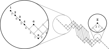
Figure 2.

∎

To prove the main results of the present paper, we need to recall some further well known facts. The following lemma is Theorem 1.6.1 of [49].

Lemma 5.

Let $G$ and $H$ be affine group schemes of finite type over ${\mathbb{Z}}$, where $G$ is flat, and let $\phi\colon G\to H$ be a morphism of group schemes. Assume that the following conditions are satisfied for an algebraically closed field $K$:

1. $\dim(G_{K})\geqslant\dim_{K}(\operatorname{Lie}(H_{K}))$,

2. $\phi$ induces monomorphisms on the groups of points $G(K)\to H(K)$ and $G(K[\delta])\to H(K[\delta])$,

3. the normalizer of $\phi(G^{0}(K))$ in $H(K)$ is contained in $\phi(G(K))$.

Then $\phi$ is an isomorphism of group schemes over ${\mathbb{Z}}$.

Here $G_{0}$ denotes the connected component of the identity in $G$, $G_{K}$ denotes the scheme obtained from $G$ by a change of scalars, and $\operatorname{Lie}(H_{K})$ denotes the Lie algebra of the scheme $H_{K}$. Recall that $K[\delta]=K[x]/(x^{2})$ is the algebra of dual numbers over $K$.

Observe, that in our case the preliminary assumptions on the schemes are satisfied automatically. All schemes considered are of finite type, being subschemes of appropriate $\operatorname{GL}_{n}$. Flatness follows from the fact that $G$ is connected and after the change of base to an algebraically closed field, we will get smooth schemes of the same dimension. Thus, we only have to verify the three conditions of the above lemma.

7. The case of an algebraically closed field

The following lemma summarizes obvious properties of the minimal representation $\pi\colon\overline{G}(\operatorname{E}_{7},-)\to\operatorname{GL}_{56}$ of the simply connected Chevalley group of type $\operatorname{E}_{7}$. The fact that $\pi(\overline{G}(\operatorname{E}_{7},-))$ is irreducible and tensor indecomposable immediately follows from the fact that $\pi$ is microweight. Its faithfulness follows from the equality of weight lattices $\Lambda(\pi)=P(\Phi)$. The claim about normalizers follows from the classical description of abstract automorphisms of Chevalley groups over fields (see [32]). Recall that this description asserts that any algebraic automorphism of an extended Chevalley group is the product of an inner automorphism, a central automorphism and a graph automorphism. The ordinary Chevalley group may have diagonal automorphisms, but they become inner in the extended group. Modulo the algebraic ones, the only non-algebraic automorphisms are field automorphisms. Clearly, groups of type $\operatorname{E}_{7}$ do not have any non-trivial graph automorphisms.

Lemma 6.

Viewed as a subgroup of $\operatorname{GL}(56,K)$, the algebraic group $\overline{G}(\operatorname{E}_{7},K)$ is irreducible and tensor indecomposable. Moreover, it is equal to its own normalizer.

Let us recall the general outline of the proof of the following lemma. It is almost the same as the proof of Lemma 10 in [43], but there is a minor difference, due to the fact that now the extended Chevalley group of type $\operatorname{E}_{7}$ is not maximal in $\operatorname{GL}(n,K)$, but is contained in the general symplectic group $\operatorname{GSp}(56,K)$. In a classical 1952 paper, Eugene Dynkin [11] described the maximal connected closed subgroups of simple algebraic groups over an algebraically closed field of characteristic 0. More precisely, he reduced their description to the representation theory of simple algebraic groups. Relying on earlier results by Seitz himself, and by Donna Testerman, Gary Seitz [31] generalized this description to subgroups of classical algebraic groups over an arbitrary algebraically closed field. Theorem 2 of [31] can be stated as follows. Let $V$ be the vector representation of $\operatorname{SL}(V)$, and $X$ be a proper simple algebraic subgroup of $\operatorname{SL}(n,K)$ such that the restriction $V|X$ of the module $V$ to $X$ is irreducible and tensor indecomposable. Further, let $Y$ be a proper connected closed subgroup of $\operatorname{SL}(n,K)$, that strictly contains $X$. Then either $Y=\operatorname{Sp}(V)$ or $Y=\operatorname{SO}(V)$, or else the pair $(X,Y)$ is explicitly listed in [31, Table 1].

Lemma 7.

Theorem 1 holds for any algebraically closed field.

Proof.

It suffices to prove that the connected components of the groups in question coincide. Since $\overline{G}(\operatorname{E}_{7},K)$ coincides with its normalizer, it will automatically follow that the group $G_{I}(K)$ is connected. The fact that $\overline{G}(\operatorname{E}_{7},K)$ stabilizes the requisite system of forms, follows from Theorem 4. The inverse inclusion can be established as follows. In Table 1 of [31] the group of type $\operatorname{E}_{7}$ occurs in the column X four times but each time in the embedding $\operatorname{E}_{7}<\operatorname{C}_{28}$. Formally, this only implies the maximality of $G(\operatorname{E}_{7},K)$ in $\operatorname{Sp}(56,K)$, rather then the maximality of $\overline{G}(\operatorname{E}_{7},K)$ in $\operatorname{GSp}(56,K)$. However, since $\det(h_{\varpi_{7}}(\eta))=\eta^{-28}$, for every algebraically closed field the determinant of $h_{\varpi_{7}}(\eta)$ can be arbitrary. Therefore, any connected closed subgroup that properly contains $\overline{G}(\operatorname{E}_{7},K)$, contains both $\operatorname{Sp}(56,K)$ and matrices of an arbitrary determinant, and thus coincides with $\operatorname{GSp}(56,K)$. It only remains to observe that the group $\operatorname{GSp}(56,K)$ does not preserve the ideal $I$. Therefore, $\overline{G}(\operatorname{E}_{7},K)$ is maximal among all such groups, and thus coincides with $G_{I}(K)$. ∎

Lemma 8.

Theorem 2 holds for any algebraically closed field.

Proof.

Completely analogous to the proof of Lemma 7, only that instead the reference to Theorem 4 one should invoke results of [25], where it is proven that $E(\operatorname{E}_{7},R)$ stabilizes the pair $(f,h)$. Therefore, $G(\operatorname{E}_{7},K)=E(\operatorname{E}_{7},K)$ is contained in $G_{(f,h)}(K)$. Moreover, it is easy to see that elements of the maximal torus $T(\operatorname{E}_{8},K)$ act as similarities of the pair $(f,h)$, and thus $\overline{G}(\operatorname{E}_{7},K)$ is contained in $\overline{G}_{(f,h)}(K)$. ∎

8. Dimension of the Lie algebra

In the present section we proceed with the proofs of Theorems 1 and 2. Namely, here we prove that the affine group schemes $G_{I}$, $G_{(f,h)}$, $\overline{G}_{(f,h)}$ are smooth. This is one of the key calculations in the present paper.

First, consider $G_{I}$. We should evaluate the dimension of the Lie algebra of this scheme. It is well known how to calculate the Lie algebra that stabilizes a system of forms, see, for instance [18]). Of course, before the advent of the theory of group schemes, in positive characteristic it was not possible to derive any information concerning the group stabilizing the same system of forms. Morally, our calculation faithfully imitates the works by William Waterhouse, especially [49], where such similar calculations were performed in Lemmas 3.2, 5.3 and 6.3. Analogous calculations for the cases of polyvector representation of $\operatorname{GL}_{n}$, and for the microweight representation of $\operatorname{E}_{6}$ were carried through in [45, 43].

Let, as above, $K$ be a field. The Lie algebra $\operatorname{Lie}((G_{I})_{K})$ of an affine group scheme $(G_{I})_{K}$ is most naturally interpreted as the kernel of the homomorphism $G_{I}(K[\delta])\longrightarrow G_{I}(K)$, sending $\delta$ to 0 see [4, 17, 38]. Let $G$ be a subscheme of $\operatorname{GL}_{n}$. Then $\operatorname{Lie}(G_{K})$ consists of all matrices of the form $e+z\delta$, where $z\in M(n,K)$, satisfying the equations defining $G(K)$. In the next lemma we specialize this statement in the case where $G$ is the stabilizer of a system of polynomials.

Lemma 9.

Let $f_{1},\ldots,f_{s}\in K[x_{1},\ldots,x_{t}]$. Then a matrix $e+z\delta$, where $z\in M(t,K)$, belongs to $\operatorname{Lie}(\operatorname{Fix}_{K}(f_{1},\ldots,f_{s}))$ if and only if

$$\sum_{1\leqslant i,j\leqslant t}z_{ij}x_{i}\frac{\partial f_{h}}{\partial x_{j}}=0,$$

for all $h=1,\ldots,s$.

The following result is proved in exactly the same way as Lemma 5.3 of [49], and as Theorem 4 of [43]. Clearly, the dimension that arises in this proof, is the dimension of the Lie algebra of type $\operatorname{E}_{7}$ increased by 1. As also in [43], from the proof it will be clear, which of the coefficients $z_{\lambda\mu}$ correspond to roots, and which correspond to the Cartan subalgebra. The extra 1 is accounted by an additional toral summand, since the Lie algebra we consider is in fact the Lie algebra of the extended Chevalley group, whose dimension exceeds dimension of the ordinary Chevalley group by 1.

Theorem 5.

For any field $K$ the dimension of the Lie algebra $\operatorname{Lie}(G_{I}(K))$ does not exceed $134$.

Proof.

Our equations take the form

$$\sum_{\lambda,\mu}z_{\lambda\mu}x_{\lambda}\frac{\partial f_{\rho,\sigma}}{\partial x_{\mu}} =0,\quad\rho,\sigma\in\Lambda,\;\rho\perp\sigma;$$

$$\sum_{\lambda,\mu}z_{\lambda\mu}x_{\lambda}\frac{\partial g_{\alpha}}{\partial x_{\mu}} =0,\quad\alpha\in\Phi.$$

Recall, that the partial derivatives look as follows:

$$\frac{\partial f_{\rho,\sigma}}{\partial x_{\mu}} =\begin{cases}\pm x_{\rho+\sigma-\mu},&\text{if $\rho+\sigma-\mu\in\Lambda$,}\\ 0,&\text{otherwise.}\end{cases}$$

$$\frac{\partial g_{\alpha}}{\partial x_{\mu}} =\begin{cases}\pm x_{\overline{\mu}},&\text{if $\mu+\alpha\in\Lambda$ of $\mu-\alpha\in\Lambda$,}\\ 0,&\text{otherwise.}\end{cases}$$

• If $d(\lambda,\mu)=3$, then $z_{\lambda\mu}=0$. Indeed, in this case $\mu=\overline{\lambda}$. There exists a root $\alpha\in\Phi$ such that $\overline{\lambda}+\alpha\in\Lambda$ or $\overline{\lambda}-\alpha\in\Lambda$. Consider the equation corresponding to the polynomial $g_{\alpha}$. It features the monomial $z_{\lambda\overline{\lambda}}x_{\lambda}\frac{\partial g_{\alpha}}{\partial x_{\overline{\lambda}}}=\pm z_{\lambda\overline{\lambda}}x_{\lambda}^{2}$. However, the monomial $x_{\lambda}^{2}$ does not occur in any generator of the ideal $I$. It follows that the coefficient $\pm z_{\lambda\overline{\lambda}}$ must be 0.

• If $d(\lambda,\mu)=2$, then $z_{\lambda\mu}=0$. Choose a root $\alpha\in\Phi$ such that $\mu+\alpha\in\Lambda$ or $\mu-\alpha\in\Lambda$. Consider the equation corresponding to the polynomial $g_{\alpha}$. It features the monomial $z_{\lambda\mu}x_{\lambda}\frac{\partial g_{\alpha}}{\partial x_{\mu}}=\pm z_{\lambda\mu}x_{\lambda}x_{\overline{\mu}}$, where $d(\lambda,\overline{\mu})=1$. Thus, the monomial $x_{\lambda}x_{\overline{\mu}}$ does not occur in any generator of the ideal $I$. The non-zero summand $\pm z_{\lambda\mu}x_{\lambda}x_{\overline{\mu}}$ could only possible cancel with the non-zero summand of the form $z_{\overline{\mu}\overline{\lambda}}x_{\overline{\mu}}\frac{\partial g_{\alpha}}{\partial x_{\overline{\lambda}}}$. However, varying $\alpha$ one can guarantee that both $\overline{\lambda}+\alpha\notin\Lambda$ and $\overline{\lambda}-\alpha\notin\Lambda$. For instance, by the transitivity of the Weyl groups on pairs of weights at distance 2, one can assume that $\lambda=\varpi_{7}$ and $\mu=\overline{\varpi}_{7}+\alpha_{7}$, in which case one can take $\alpha=\alpha_{6}$. For this choice of $\alpha$ the summand $\pm z_{\lambda\mu}x_{\lambda}x_{\overline{\mu}}$ remains the summand containing $x_{\lambda}x_{\overline{\mu}}$, and thus $z_{\lambda\mu}=0$.

• If $d(\lambda,\mu)=d(\nu,\rho)=1$ and $\lambda-\mu=\nu-\rho$, then $z_{\lambda\mu}=\pm z_{\nu\rho}$. First, assume that $(\nu,\rho)\neq(\overline{\mu},\overline{\lambda})$. In this case, $\lambda\perp\rho$, $\mu\perp\nu$ and $\lambda+\rho=\mu+\nu$. Consider the equation corresponding to the polynomial $f_{\lambda,\rho}=f_{\mu,\nu}$. It features the monomials $z_{\lambda\mu}x_{\lambda}\frac{\partial f_{\lambda,\rho}}{\partial x_{\mu}}=\pm z_{\lambda\mu}x_{\lambda}x_{\nu}$ and $z_{\nu\rho}x_{\nu}\frac{\partial f_{\lambda,\rho}}{\partial x_{\rho}}=\pm z_{\nu\rho}x_{\nu}x_{\lambda}$. However, $d(\lambda,\nu)=1$, so that the monomial $x_{\lambda}x_{\nu}$ does not occur in any generator of the ideal $I$. This means that these two monomials must sum to $0$, so that $z_{\lambda\mu}=\pm z_{\nu\rho}$.

• If $d(\lambda,\mu)=d(\nu,\rho)=1$ and $\lambda-\mu=\nu-\rho$, then $z_{\rho\rho}=\pm z_{\lambda\lambda}\pm z_{\mu\mu}\pm z_{\nu\nu}$. Indeed, the equation corresponding to the same polynomial $f_{\lambda,\rho}=f_{\mu,\nu}$, as in the preceding item, features monomials $z_{\lambda\lambda}x_{\lambda}\frac{\partial f_{\lambda,\rho}}{\partial x_{\lambda}}=\pm z_{\lambda\lambda}x_{\lambda}x_{\rho}$, $z_{\mu\mu}x_{\mu}\frac{\partial f_{\lambda,\rho}}{\partial x_{\mu}}=\pm z_{\mu\mu}x_{\mu}x_{\nu}$, $z_{\nu\nu}x_{\nu}\frac{\partial f_{\lambda,\rho}}{\partial x_{\nu}}=\pm z_{\nu\nu}x_{\nu}x_{\mu}$, and $z_{\rho\rho}x_{\rho}\frac{\partial f_{\lambda,\rho}}{\partial x_{\rho}}=\pm z_{\rho\rho}x_{\rho}x_{\lambda}$. Observe, that the monomial $x_{\lambda}x_{\rho}$ occurs in exactly one of the generators of $I$, viz. in $f_{\lambda,\rho}$), and $x_{\mu}x_{\nu}$ occurs in the same polynomial, with the same coefficient, up to sign. Equating the coefficients of the above monomials, we see $z_{\lambda\lambda}\pm z_{\rho\rho}=\pm z_{\mu\mu}\pm z_{\nu\nu}$.

Let us summarize what we have just established. The first two items show that the matrix entries $z_{\lambda\mu}$ with $d(\lambda,\mu)\geqslant 2$ do not contribute to the dimension of the Lie algebra, whereas the entries $z_{\lambda\mu}$ with $d(\lambda,\mu)=1$ give the contribution equal to the number of roots of $\Phi$, namely, $126$. Finally, the last item allows us to express all entries $z_{\lambda\lambda}$ as linear combinations of the entries $z_{\mu\mu}$, for $\mu=\mu_{1},\dots,\mu_{t}$, such that each fundamental root of $\Phi$ occurs among the pair-wise differences of the weights $\mu_{i}$. It is easy to see that the smallest number of such weights is 8, and that one can use the weights $1,2,3,4,5,6,7,8$ as such. Figure 3 shows their location in the weight diagram.

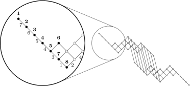
Figure 3.

Thus, the dimension of the Lie algebra does not exceed $126+8=134$. ∎

Next, we pass to the schemes $G_{(f,h)}$ and $\overline{G}_{(f,h)}$. As above, we can identify the Lie algebras $\operatorname{Lie}(G_{(f,h)}(K))$ and $\operatorname{Lie}(\overline{G}_{(f,h)}(K))$ with the kernels of homomorphisms obtained by specializing $\delta$ in the ring of dual numbers $K[\delta]$ to 0. Thus, $\operatorname{Lie}(G_{(f,h)}(K))$ consists of the matrices $g=e+x\delta$, where $x\in M(n,K)$, satisfying the following conditions: $f(gu,gv,gw,gz)=f(u,v,w,z)$ and $h(gu,gv)=h(u,v)$, for all $u,v,w,z\in V$. Similarly, $\operatorname{Lie}(\overline{G}_{(f,h)}(K))$ consists of all matrices $g=e+x\delta$, where $x\in M(n,K)$, satisfying the conditions $f(gu,gv,gw,gz)=\varepsilon(g)f(u,v,w,z)$ and $h(gu,gv)=\varepsilon^{2}(g)h(u,v)$ for all $u,v,w,z\in V$.

Theorem 6.

For any field $K$ the dimension of the Lie algebra $\operatorname{Lie}(G_{(f,h)}(K))$ does not exceed $133$, while the dimension of the Lie algebra $\operatorname{Lie}(\overline{G}_{(f,h)}(K))$ does not exceed $134$.

Proof.

First, observe that the conditions on elements of the Lie algebra $\operatorname{Lie}(G_{(f,h)}(K))$ are obtained from the corresponding conditions for elements of $\operatorname{Lie}(\overline{G}_{(f,h)}(K))$ by substituting $\varepsilon(g)=\varepsilon^{\prime}(g)=1$ and $c_{2}(g)=c_{3}(g)=c_{4}(g)=0$. Let $g$ be a matrix satisfying the above conditions for all $u,v,w,z\in V$. Plugging in $g=e+x\delta$ and using that the form $f$ is four-linear, whereas the form $h$ is bilinear, we get

$$f(xu,v,w,z) +f(u,xv,w,z)+f(u,v,xw,z)+f(u,v,w,xz)$$

$$=(\varepsilon(g)-1)f(u,v,w,z)+c_{2}(g)h(u,v)h(w,z)$$

$$\quad+c_{3}(g)h(u,w)h(v,z)+c_{4}(g)h(u,z)h(v,w)$$

and

$$h(xu,v)+h(u,xv) =(\varepsilon^{\prime}(g)-1)h(u,v).$$

Now we show that the entries of the matrix $x$ are subject to exactly the same linear dependences, as in the proof of Theorem 5.

• If $d(\lambda,\mu)=3$, then $x_{\lambda\mu}=0$. Indeed, in this case $\mu=\overline{\lambda}$. Let $(\lambda,\rho,\sigma,\tau)$ be a non-degenerate quadruple of weights containing $\lambda$. Set $u=e_{\rho}$, $v=e_{\sigma}$, $w=e_{\tau}$, $z=e_{\mu}$. Then $(\rho,\mu)=(\rho,\delta-\lambda)=(\rho,\delta)=1/2$. Similarly, $(\sigma,\mu)=(\tau,\mu)=1/2$. This means that $\mu$ is not orthogonal and not opposite to any of the weights $\rho,\sigma,\tau$. Thus $f(xu,v,w,z)=f(u,xv,w,z)=f(u,v,xw,z)=f(u,v,w,z)=0$. It follows that $f(u,v,w,xz)=\pm x_{\lambda\mu}=0$.

• If $d(\lambda,\mu)=2$, then $x_{\lambda\mu}=0$. Let $\{\lambda\}^{\perp}\subseteq\Lambda$ be the set of weights orthogonal to $\lambda$. Observe that $\mu\in\{\lambda\}^{\perp}$. Moreover, $|\{\lambda\}^{\perp}|=27$, and these weights are the weights of the $27$-dimensional representation of the Chevalley group of type $\operatorname{E}_{6}$. Take in $\{\lambda\}^{\perp}$ three weight $\rho,\sigma,\tau$ forming a triad (i.e. pair-wise orthogonal) in such a way that $\mu\notin\{\rho,\sigma,\tau\}$. Then $(\lambda,\rho,\sigma,\tau)$ is a non-degenerate quadruple of weights. Set $u=e_{\rho}$, $v=e_{\sigma}$, $w=e_{\tau}$, $z=e_{\mu}$. Observe that $\mu$ cannot be orthogonal to more than one of the weights $\rho,\sigma,\tau$. Indeed, let $\mu$ be orthogonal to two of them, say $\mu\perp\rho$ and $\mu\perp\sigma$. Since $\mu\in\{\lambda\}^{\perp}$, and in $\{\lambda\}^{\perp}$ there is a unique weight that is orthogonal to both $\rho$ and $\sigma$, namely, $\tau$. It follows that $\mu=\tau$, a contradiction. Thus, $f(xu,v,w,z)=f(u,xv,w,z)=f(u,v,xw,z)=f(u,v,w,z)=0$. It follows that $f(u,v,w,xz)=\pm x_{\lambda\mu}=0$.

• If $d(\lambda,\mu)=1$ and $\lambda-\mu=\nu-\rho$, then $x_{\lambda\mu}=\pm x_{\nu\rho}$. By the transitivity of the action of the Weyl group on the pairs of weights at distance 1, we can move the pair $(\lambda,\mu)$ to the pair $(1,2)$. Then $\nu-\rho=\alpha_{7}$. In the weight diagram there are exactly $12$ edges marked $7$, which gives us exactly $12$ possibilities for the pair $(\nu,\rho)$. This leaves us with the following three cases to examine:

  1. $(\nu,\rho)=(\lambda,\mu)$;

  2. $d(\lambda,\rho)=2$;

  3. $(\nu,\rho)=(\overline{\mu},\overline{\lambda})$.

  The first of these cases is trivial. Next, we observe that is suffices to prove the equality $x_{\lambda\mu}=\pm x_{\nu\rho}$ for the second case, and then to use the chain of equalities $x_{\lambda\mu}=\pm x_{\nu\rho}=\pm x_{\overline{\mu}\overline{\lambda}}$ to derive the third case. Thus, we are left with the analysis of the situation, where $d(\lambda,\rho)=2$. There exists a non-degenerate quadruple of weights $(\lambda,\rho,\sigma,\tau)$. Furthermore, we can stipulate that $d(\mu,\sigma)=2$. Indeed, in the case $\lambda=\lambda_{1}$, $\mu=\lambda_{2}$, $\rho=\lambda_{\overline{16}}$, the choice $\sigma=\lambda_{\overline{15}}$, $\tau=\lambda_{\overline{14}}$ would do. Now, set $u=e_{\mu}$, $v=e_{\rho}$, $w=e_{\sigma}$, $z=e_{\tau}$. Then $d(\mu,\rho)=1$, and thus $f(u,v,xw,z)=f(u,v,w,xz)=f(u,v,w,z)=0$. It follows that $f(xu,v,w,z)+f(u,xv,w,z)=0$. But $f(xu,v,w,z)=\pm x_{\lambda\mu}$ and $f(u,xv,w,z)=\pm x_{\nu\rho}$.

• If $d(\lambda,\mu)=1$ and $\lambda-\mu=\nu-\rho$, then $x_{\lambda\lambda}-x_{\mu\mu}=x_{\nu\nu}-x_{\rho\rho}$. As in the proof of the preceding item, we can limit ourselves with the analysis of the case, where $d(\lambda,\rho)=2$. Again we can find a non-degenerate quadruple of weights $(\lambda,\rho,\sigma,\tau)$ such that $d(\mu,\sigma)=2$. Setting $u=e_{\lambda}$, $v=e_{\rho}$, $w=e_{\sigma}$, $z=e_{\tau}$, we get $(x_{\lambda\lambda}+x_{\rho\rho}+x_{\sigma\sigma}+x_{\tau\tau}-\varepsilon(g)+1)f(e_{\lambda},e_{\rho},e_{\sigma},e_{\tau})=0$. It follows that $x_{\lambda\lambda}+x_{\rho\rho}+x_{\sigma\sigma}+x_{\tau\tau}=\varepsilon(g)-1$. On the other hand, $(\mu,\nu,\sigma,\tau)$ is another non-degenerate quadruple. Setting $u=e_{\mu}$, $v=e_{\nu}$, $w=e_{\sigma}$, $z=e_{\tau}$, we get $(x_{\mu\mu}+x_{\nu\nu}+x_{\sigma\sigma}+x_{\tau\tau}-\varepsilon(g)+1)f(e_{\mu},e_{\nu},e_{\sigma},e_{\tau})=0$. It follows that $x_{\mu\mu}+x_{\nu\nu}+x_{\sigma\sigma}+x_{\tau\tau}=\varepsilon(g)-1$. Comparing these expressions, we can conclude that $x_{\lambda\lambda}-x_{\mu\mu}=x_{\nu\nu}-x_{\rho\rho}$.

Thus, as in the proof of Theorem 5, it turns out that the dimension of the Lie algebra $\operatorname{Lie}(\overline{G}_{(f,h)}(K))$ does not exceed $126+8=134$. The same arguments are also applicable for the case of $\operatorname{Lie}(G_{(f,h)}(K))$. It suffices to set $\varepsilon(g)=\varepsilon^{\prime}(g)=1$ and $c_{2}(g)=c_{3}(g)=c_{4}(g)=0$. Again, we can conclude that the dimension of $\operatorname{Lie}(G_{(f,h)}(K))$ does not exceed $134$: the entries $x_{\lambda\mu}$ do not contribute to the dimension when $d(\lambda,\mu)\geqslant 2$, they make a contribution $126$, when $d(\lambda,\mu)=1$, and, finally, they make a contribution $\leqslant 8$, for $d(\lambda,\mu)=0$.

To conclude the proof of the theorem, we have to find a non-trivial relation among these last entries. From the final paragraph of the proof of Theorem 5) we know that the entries $z_{\lambda\lambda}$ are linear combinations of 8 of them, namely $z_{\mu\mu}$, for $\mu=\mu_{1},\dots,\mu_{8}$. Here, as $\mu_{1},\dots,\mu_{8}$ one can takes the weights $1,2,3,4,5,6,7,8$, respectively. Now, set $u=e_{\mu_{1}}$, $v=e_{\overline{\mu_{1}}}$. Plugging these entries into the equation $h(xu,v)+h(u,xv)=0$, we get that $x_{\mu_{1}\mu_{1}}+x_{\overline{\mu_{1}}\overline{\mu_{1}}}=0$. One the other hand, $\mu_{1}-\overline{\mu_{1}}=\delta=(2\alpha_{1}+3\alpha_{2}+4\alpha_{3}+6\alpha_{4}+5\alpha_{5}+4\alpha_{6}+3\alpha_{7})$, and thus the relations $x_{\lambda\lambda}-x_{\mu\mu}=x_{\nu\nu}-x_{\rho\rho}$ for $\lambda-\mu=\nu-\rho\in\Phi$ imply that

$$x_{\mu_{1}\mu_{1}}-x_{\overline{\mu_{1}}\overline{\mu_{1}}} =2(x_{\mu_{7}\mu_{7}}-x_{\mu_{8}\mu_{8}})+3(x_{\mu_{5}\mu_{5}}-x_{\mu_{6}\mu_{6}})$$

$$\quad+4(x_{\mu_{5}\mu_{5}}-x_{\mu_{7}\mu_{7}})+6(x_{\mu_{4}\mu_{4}}-x_{\mu_{5}\mu_{5}})$$

$$\quad+5(x_{\mu_{3}\mu_{3}}-x_{\mu_{4}\mu_{4}})+4(x_{\mu_{2}\mu_{2}}-x_{\mu_{3}\mu_{3}})$$

$$\quad+3(x_{\mu_{1}\mu_{1}}-x_{\mu_{2}\mu_{2}})$$

$$=3x_{\mu_{1}\mu_{1}}+x_{\mu_{2}\mu_{2}}+x_{\mu_{3}\mu_{3}}+x_{\mu_{4}\mu_{4}}$$

$$\quad+x_{\mu_{5}\mu_{5}}-3x_{\mu_{6}\mu_{6}}-2x_{\mu_{7}\mu_{7}}-2x_{\mu_{8}\mu_{8}}.$$

Comparing this with the equality $x_{\mu_{1}\mu_{1}}+x_{\overline{\mu_{1}}\overline{\mu_{1}}}=0$, we get that $x_{\mu_{1}\mu_{1}}+x_{\mu_{2}\mu_{2}}+x_{\mu_{3}\mu_{3}}+x_{\mu_{4}\mu_{4}}+x_{\mu_{5}\mu_{5}}-3x_{\mu_{6}\mu_{6}}-2x_{\mu_{7}\mu_{7}}-2x_{\mu_{8}\mu_{8}}=0$. This is precisely the desired non-trivial linear relation among the elements $x_{\mu_{i}\mu_{i}}$, which, over a field of any characteristic, shows that the dimension of our Lie algebra is $1$ smaller than the above bound. Thus, $\dim\operatorname{Lie}(G_{(f,h)}(K))\leqslant 133$, as claimed. ∎

9. Proofs of Theorems 1 and 2

Now we are all set to finish the proofs of our main results.

Proof of Theorem 1.

Consider the rational representation of algebraic groups

$$\pi\colon\overline{G}(\operatorname{E}_{7},{-})\to\operatorname{GL}_{56}$$

with the highest weight $\varpi_{7}$. This representation is faithful, and by Theorem 4 its image is contained in $G_{I}$. We wish to apply to this morphism $\pi$ Lemma 5.

Indeed, for an algebraically closed field $K$ and for $K[\delta]$ the representation $\pi$ is a monomorphism. This means that the condition 2 of Lemma 5 holds. Clearly, $\dim(\overline{G}(\operatorname{E}_{7},K))=134$, and Theorem 5 implies that also $\dim_{K}(\operatorname{Lie}(G_{K}))\leqslant 134$, so that the condition 1 of Lemma 5 follows from the fact that by Lemma 6 already the normalizer of $\overline{G}(\operatorname{E}_{7},K)$ in $\operatorname{GL}(56,K)$ is contained in — and in fact coincides with — $G_{I}(K)$. This means that we can apply Lemma 5 to conclude that $\pi$ establishes an isomorphism of $\overline{G}(\operatorname{E}_{7},{-})$ and $G_{I}$, as affine group schemes over ${\mathbb{Z}}$. ∎

Proof of Theorem 2.

Here again we can use Lemma 5. The situation is completely analogous to the proof of Theorem 1, only that instead of reference to Theorem 4, one should invoke the main theorem of [25], and instead of Theorem 5 one should use Theorem 6. ∎

Lemma 10.

In the definition of the group $\overline{G}_{(f,h)}(R)$ always $\varepsilon^{\prime}(g)=(\varepsilon(g))^{2}$ and $c_{2}(g)=c_{3}(g)=c_{4}(g)=0$. In other words,

$$\overline{G}_{(f,h)}(R) =\{g\in\operatorname{GL}(56,R)\mid\text{ there exists $\varepsilon\in R^{*}$ such that }$$

$$\qquad f(gu,gv,gw,gz)=\varepsilon f(u,v,w,z)$$

$$\qquad\text{and }h(gu,gv)=\varepsilon^{2}h(u,v)\text{ for all }u,v,w,z\in V\}.$$

Proof.

We have already shown that the group $\overline{G}_{(f,h)}(R)$ coincides with the extended Chevalley group $\overline{G}(\operatorname{E}_{7},R)$. Clearly, both $\varepsilon$ and $\varepsilon^{\prime}$ are homomorphisms from $\overline{G}(\operatorname{E}_{7},{-})$ to $\mathbb{G}_{m}$, trivial on the commutator subgroup. Thus, their appropriate powers should coincide. Calculating their values on the semi-simple element $h_{\varpi_{7}}(\eta)$, we see that $\varepsilon$ takes the value $\eta^{2}$, whereas $\varepsilon^{\prime}$ takes the value $\eta$. Thus, $\varepsilon=(\varepsilon^{\prime})^{2}$.

On the other hand, it is easy to see that $c_{i}$ enjoy the 1-cocycle identity $c_{i}(gh)=\varepsilon(g)c_{i}(h)+c_{i}(g)\varepsilon(h)$ and vanish on both the commutator subgroup and the semi-simple elements of the form $h_{\varpi_{7}}(\eta)$. As an algebraic group, the extended Chevalley group is generated by these two subgroups, so that $c_{i}$ are identically 0. ∎

10. Proof of Theorem 3

Proof of Theorem 3.

Clearly, $\overline{G}(\operatorname{E}_{7},R)\leqslant N(G(\operatorname{E}_{7},R))$. It is well known, see, for instance [16]) and references there, that for any irreducible root system $\Phi$ of rank strictly larger than 1, and for any commutative ring $R$ the elementary group $E(\Phi,R)$ is normal in the extended Chevalley group $\overline{G}(\Phi,R)$. Therefore, $\overline{G}(\operatorname{E}_{7},R)\leqslant N(E(\operatorname{E}_{7},R))$. On the other hand, both normalizers $N(E(\operatorname{E}_{7},R))$ and $N(G(\operatorname{E}_{7},R))$ are obviously contained in the transporter $\operatorname{Tran}(E(\operatorname{E}_{7},R),G(\operatorname{E}_{7},R))$. Thus, to finish the proof of the theorem, it suffices to verify that $\operatorname{Tran}(E(\operatorname{E}_{7},R),G(\operatorname{E}_{7},R))$ is contained in $\overline{G}(\operatorname{E}_{7},R)$.

Let $g\in\operatorname{GL}(56,R)$ belong to $\operatorname{Tran}(E(\operatorname{E}_{7},R),G(\operatorname{E}_{7},R))$. WE pick any root $\alpha\in\Phi$ and any $\xi\in R$. Then $a=gx_{\alpha}(\xi)g^{-1}$ lies in $G(\operatorname{E}_{7},R)$, and thus $f(au,av,aw,az)=f(u,v,w,z)$ and $h(au,av)=h(u,v)$ for all $u,v,w,z\in V$. Therefore, substituting $(gu,gv,gw,gz)$ for $(u,v,w,z)$, we get

$$f(gx_{\alpha}(\xi)u,gx_{\alpha}(\xi)v,gx_{\alpha}(\xi)w,gx_{\alpha}(\xi)z)$$

$$\quad=f(gu,gv,gw,gz)\text{ for all }u,v,w,z\in V.$$

Consider the form $F\colon V\times V\times V\times V\to R$, defined by

$$F(u,v,w,z)=f(gu,gv,gw,gz).$$

By our assumption, one has

$$F(x_{\alpha}(\xi)u,x_{\alpha}(\xi)v,x_{\alpha}(\xi)w,x_{\alpha}(\xi)z)=F(u,v,w,z)$$

for all $u,v,w,z\in V$ and for all $\alpha\in\Phi$, $\xi\in R$. Root unipotents $x_{\alpha}(\xi)$ generate the elementary group $E(\operatorname{E}_{7},R)$. It follows that the form $F$ is invariant under the action of this group. Obviously, the form $F$ is four-linear. Thus, we can apply to this form the main result of [25, Theorem 2]). It says that in this case the form $F$ has the shape

$$F(u,v,w,z) =\varepsilon f(u,v,w,z)+c_{2}h(u,v)h(w,z)$$

$$+c_{3}h(u,w)h(v,z)+c_{4}h(u,z)h(v,w),$$

for some $\varepsilon,c_{2},c_{3},c_{4}\in R$. Plugging in $g^{-1}$ instead of $g$, we can conclude that $\varepsilon\in R^{*}$.

A similar calculation for $h$ shows that $h(gu,gv)=\varepsilon^{\prime}h(u,v)$ for some $\varepsilon^{\prime}\in R$. Again, plugging in $g^{-1}$ instead of $g$, we can conclude that $\varepsilon^{\prime}\in R^{*}$.

This shows that $g$ belongs to the group $\overline{G}_{(f,h)}(R)$, which by Theorem 2 coincides with $\overline{G}(\operatorname{E}_{7},R)$. ∎

The authors are grateful to Ernest Borisovich Vinberg, who pointed out a serious error in a preliminary version of this paper. Also, the authors are grateful to the referee, for the statement and proof of Lemma 10.

References

- [1]
- [2] Aschbacher M., Some multilinear forms with large isometry groups, Geom. Dedicata 25 (1988), no. 1-3, 417–465.
- [3] Berman S., Moody R. V., Extensions of Chevalley groups, Israel J. Math. 22 (1975), no. 1, 42–51.
- [4] A. Borel, Properties and linear representations of Chevalley groups, Seminar on Algebraic Groups and Related Finite Groups, Lecture Notes in Math., vol. 131, Springer, Berlin, 1970, pp. 1–55.
- [5] N. Bourbaki, Éléments de Mathématique. Fasc. XXXIV. Groupes et algèbres de Lie. Chapitres IV á VI, Actualités Scientifiques et Industrielles, No. 1337, Hermann. Paris, 1968.
- [6] Brown R. B., Groups of type , J. Reine Angew. Math. 236 (1969), 79–102.
- [7] E. I. Bunina, Automorphisms of Chevalley groups of types , , and over local rings with , Fundam. Prikl. Mat. 15 (2009), no. 2, 35–59; English transl., J. Math. Sci. (N. Y.) 167 (2010), no. 6, 749–766.
- [8] C. Chevalley, Sur certains groupes simples, Tohoku Math. J. (2) 7 (1955), no. 1, 14–66.
- [9] Cooperstein B. N., The fifty-six-dimensional module for . I. A four form for , J. Algebra 173 (1995), no. 2, 361–389.
- [10] Dixon J. D., Rigid embedding of simple groups in the general linear group, Canad. J. Math. 29 (1977), no. 2, 384–391.
- [11] E. B. Dynkin, Maximal subgroups of classical groups, Tr. Moscov. Mat. Obshch. 1 (1952), 39–166. (Russian)
- [12] Faulkner J. R., Ferrar J. C., Exceptional Lie algebras and related algebraic and geometric structures, Bull. London Math. Soc. 9 (1977), no. 1, 1–35.
- [13] Freudenthal H., Sur le groupe exceptionnel , Proc. Nederl. Akad. Wetensch. Ser. A 56 (1953), 81–89.
- [14] Freudenthal H., Beziehungen der und zur Oktavenebene, I–XI, Proc. Nederl. Akad. Wetensch. Ser. A 57 (1954), 218–230, 363–368; 58 (1955), 151–157, 277–285; 62 (1959), 165–201, 447–474; 66 (1963), 457–487.
- [15] Haris S. J., Some irreducible representations of exceptional algebraic groups, Amer. J. Math. 93 (1971), no. 1, 75–106.
- [16] Hazrat R., Vavilov N., of Chevalley groups are nilpotent, J. Pure Appl. Algebra 179 (2003), no. 1–2, 99–116.
- [17] J. E. Humphreys, Linear algebraic groups, Grad. Texts in Math., vol. 21, Springer-Verlag, New York–Heidelberg, 1975. MR 0396773 (53:633)
- [18] Jacobson N., Structure and representations of Jordan algebras, Amer. Math. Soc. Colloq. Publ., vol. 39, Amer. Math. Soc., Providence, RI., 1968.
- [19] Lichtenstein W., A system of quadrics describing the orbit of the highest weight vector, Proc. Amer. Math. Soc 84 (1982), no. 4, 605–608.
- [20] Liebeck M. W., Seitz G. M., On the subgroup structure of exceptional groups of Lie type, Trans. Amer. Math. Soc. 350 (1998), no. 9, 3409–3482.
- [21] Lurie J., On simply laced Lie algebras and their minuscule representations, Comment. Math. Helv. 166 (2001), no. 3, 515–575.
- [22] A. Yu. Luzgarev, On overgroups of and in their minimal representations, J. Math. Sci. (N.Y.) 134 (2006), no. 6, 2558–2571.
- [23] A. Yu. Luzgarev, Overgroups of exceptional groups, Kand. diss., S.-Petersburg. Univ., SPb, 2008. (Russian).
- [24] A. Yu. Luzgarev, Overgroups of in over commutative rings, St. Petersburg. Math. J. 20 (2009), no. 6, 955–981.
- [25] A. Yu. Luzgarev, Fourth-degree invariants for not depending on the characteristic, Vestn. St. Petersbg. Univ., Math. 46 (2013), no. 1, pp. 29–34.
- [26] Luzgarev A., Equations determining the orbit of the highest weight vector in the adjoint representation, http://arxiv:1401.0849.
- [27] Luzgarev A., Petrov V., Vavilov N., Explicit equations on orbit of the highest weight vector. (to appear)
- [28] Matsumoto H., Sur les sous-groupes arithmétiques des groupes semi-simples déployés, Ann. Sci. École Norm. Sup. (4) 2 (1969), 1–62.
- [29] Petrov V., Overgroups of unitary groups, -Theory 29 (2003), no. 3, 147–174.
- [30] Plotkin E. B., Semenov A. A., Vavilov N. A., Visual basic representations: an atlas, Internat. J. Algebra Comput. 8 (1998), no. 1, 61–95.
- [31] Seitz G. M., The maximal subgroups of classical algebraic groups, Mem. Amer. Math. Soc. 67 (1987), no. 365.
- [32] Stein M. R., Generators, relations and coverings of Chevalley groups over commutative rings, Amer. J. Math. 93 (1971), 965–1004.
- [33] Stein M. R., Stability theorems for , and related functors modeled on Chevalley groups, Japan. J. Math. (N.S.) 4 (1978), no. 1, 77–108.
- [34] N. A. Vavilov, Weight elements of Chevalley groups, Soviet Math. Dokl. 37 (1988), no. 1, 92–95.
- [35] N. A. Vavilov, Subgroups of Chevalley groups containing a maximal torus, Proceedings of the St. Petersburg Mathematical Society, 1 (1990), AMS Translations (series 2), 55–100.
- [36] Vavilov N. A., Structure of Chevalley groups over commutative rings, Nonassociative Algebras and Related Topics (Hiroshima, 1990), World Sci. Publ., River Edge, NJ, 1991, pp. 219–335.
- [37] Vavilov N. A., A third look at weight diagrams, Rend. Sem. Mat. Univ. Padova 104 (2000), 201–250.
- [38] Vavilov N. A., An -proof of structure theorems for Chevalley groups of types and , Internat. J. Algebra Comput. 17 (2007), no. 5-6, 1283–1298.
- [39] N. A. Vavilov, Can one see the signs of structure constants? St. Petersburg Math. J. 19 (2008), no. 4, 519–543.
- [40] N. A. Vavilov, Weight elements of Chevalley groups, St. Petersburg Math. J. 20 (2009), no. 1, 23–57.
- [41] N. A. Vavilov, Numerology of square equations, St. Petersburg Math. J. 20 (2009), no. 5, 687–707.
- [42] N. A. Vavilov, Some more exceptional numerology, J. Math. Sci. (N. Y.) 171 (2010), no. 3, 317–321.
- [43] N. A. Vavilov A. Yu. Luzgarev, Normalizer of the Chevalley group of type , St. Petersburg. Math. J. 19 (2008), no. 5, 699–718.
- [44] N. A. Vavilov A. Yu. Luzgarev, Chevalley groups of type in the -dimensional representation, J. Math. Sci. 180 (2012), no. 3, 197–251.
- [45] N. A. Vavilov E. Ya. Perel’man, Polyvector representations of , J. Math. Sci. (N. Y.) 145 (2007), no. 1, 4737–4750.
- [46] N. A. Vavilov V. A. Petrov, On overgroups of , St. Petersburg. Math. J. 15 (2004), no. 4, 515–543.
- [47] N. A. Vavilov V. A. Petrov, On overgroups of , St. Petersburg. Math. J. 19 (2008), no. 2, 167–195.
- [48] Vavilov N. A., Plotkin E. B., Chevalley groups over commutative rings. I. Elementary calculations, Acta Appl. Math. 45 (1996), no. 1, 73–113.
- [49] Waterhouse W. C., Automorphisms of : the group scheme approach, Adv. in Math. 65 (1987), no. 2, 171–203.