Limitations for nonlinear stabilization over uncertain channel

Abstract

We study the problem of mean-square exponential incremental stabilization of nonlinear systems over uncertain communication channels. We show the ability to stabilize a system over such channels is fundamentally limited and the channel uncertainty must provide a minimal Quality of Service (QoS) to support stabilization. The smallest QoS necessary for stabilization is shown as a function of the positive Lyapunov exponents of uncontrolled nonlinear systems. The positive Lyapunov exponent is a measure of dynamical complexity and captures the rate of exponential divergence of nearby system trajectories. One of the main highlights of our results is the role played by nonequilibrium dynamics to determine the limitation for incremental stabilization over networks with uncertainty.

1 Introduction

Networked controlled systems have been the focus of much research in recent years [1, 2, 3, 4, 5, 6, 7, 8, 9, 10, 11]. Among several relevant questions, one main problem is to characterize the limitations of closed loop stability and performance induced by the presence of unreliable communication channel(s) in the loop.

The vast majority of the studies have focused on Linear Time-Invariant (LTI) plants under a variety of settings and assumptions. Tatikonda and Mitter [12] has considered finite-rate channels and showed the required communication rate for stabilization is function of the unstable eigenvalues of the plant. Sahai [4] considered noisy channel models and showed a new notion of reliable communication, different than Shannon’s, is required to obtain the moment stability of the closed loop. Besides making clear that different notions of stability may require different notions of reliable communication in the context of a simple binary erasure channel, [4] has identified fading in the channel rather than its discrete nature, a main source of limitation for reliable communication. In fact, the binary erasure channel can be thought of as a 1-bit finite-rate channel with extreme $0-1$ fading. The focus on fading has lead to the introduction of analog erasure channels, which we consider in this paper, where the quantization effects are neglected and the channel is modeled as a random independent Bernoulli switch [5, 6, 8]. This model and its generalization to Markovian-dependent switches is a simple, yet effective, model for packet-drops links, and allows study of the stability limitations induced by these channels in the limit of large packet length, using classical stochastic systems techniques and tools. It is difficult to summarize the plethora of research in the area of control of LTI systems involving an independent, identically distributed (IID) Bernoulli switch. The notion of stability, the location of the channel(s) (at the sensor or actuator side or both) [13, 14, 15], the information available to encoders and decoders (like channel state information (CSI) or knowledge of other signals in the loop) and their computational power [13, 16], and, of course, other performance objectives [17, 15, 18] affect the required minimal Quality of Service (probability of successful delivery of the packets) by the communication link. For example, in the case of one channel on the sensor side with mean-square stability, no encoding, and CSI used at the decoder, the QoS is a function of all the unstable eigenvalues of the plant [19]. If a Kalman filter, which uses the plant input, is allowed as an encoder and the entire estimated state of the system is sent over the channel, then the minimal QoS is only a function of the plant’s eigenvalues of the largest magnitude [16]. Finally, if no encoder is allowed and the stability notion is of bounded second moment instead, then the limitation is not completely characterized, and the QoS is bounded between the previous two cases [7, 19]. While the picture is fragmented, at the same time it is clear, channel fading fundamentally limits the ability to stabilize the networked system, at least in term of moments.

For completeness, we point out a current body of literature on the related problem of state estimation over noisy channels; see, for example, [7, 20, 21]. When the erasure channel is on the sensor side, like in the estimation problems, the development is somewhat simplified because the channel state is available at the receiver side and can be included in the design of the estimator [7]. In this case, the design approach for Markovian Jump Linear Systems (MJLS) [22] can be quite useful, [6, 23]. When the channel is on the actuator side, the problem is more involved, as the controller and the decoder, which can use the CSI, are physically separated and their design is decentralized, in general. Excluding some special cases [19], the controller cannot be an instantaneous function of the channel state. For example in this paper’s setup this makes therefore the MJLS design unamenable to this problem.

While there are many results involving the stabilization of linear systems over communication networks, little has been developed for nonlinear systems with the notable exception by [24, 25]. The analysis of the limitations for the stabilization of nonlinear systems is reduced through linearization or through robust control theory to the linear case involving the eigenvalues of the linearized system. The results in [24] and [25] have connected the limits for stabilization with topological and measure theoretic (or metric) entropy corresponding to equilibrium dynamics, respectively. Even less work has considered fading channels [26, 27]. In [27], the limitation of stabilization for a scalar nonlinear system over the fading channel is studied to provide a necessary condition for general $q^{th}$ moment stabilization. The various proofs involved in the vector case are fundamentally different and cannot be trivially extended from the scalar case. Similarly [26, 28, 29], developed along with this paper, considered the estimation and stabilization problem and used many of the ideas developed in this paper. However, the distinctive feature of the stabilization problem is the limitations for stabilization are shown to be offered by two competing local and global dynamics of the system. Furthermore, unlike results in [26, 28], results in this paper are proved under the noncompact assumption on the state space and in the presence of additive noise term. In this paper, we also consider more general channel uncertainty model as opposed to Bernoulli (on-off) channel uncertainty considered in [26, 28]. Establishing connection between various notions of stabilities, in particular the incremental mean square and bounded second moment stability for nonlinear systems evolving on unbounded state space, also form one of the main contributions of this paper.

In this paper, we fill the gap and study the limitations of the stabilization for a class of nonlinear unstable systems over general uncertain channels. We consider a set-up sufficiently simple to allow characterization of the limitations and, at the same time, not too unrealistic. We assume the controller has perfect access to the plant’s state. However, it can act on the plant’s input through an uncertain channel. Moreover, on the receiver’s side, there is no sophisticated decoder that exploits the CSI. This is a simplified model of a User Datagram Protocol (UDP)-like or best effort protocol [15]. While more complex schemes can be studied using our approach, their investigation is outside the scope of this paper. The main contribution of this paper is to show the open loop, nonequilibrium dynamics of the plant also imposes minimal requirements on the QoS of the link, together with the local instability of the equilibrium point. This represents an important departure from local equilibrium results and shows the relevance of nonequilibrium dynamics. In particular, it shows a failure to allocate QoS to the unstable nonequilibrium dynamics and only focus on the unstable equilibrium dynamics can have disastrous consequences. Thus, the problem of characterizing the limitations of the stabilization and estimation of network nonlinear systems over noisy, uncertain channels is a timely research topic, given the important role that nonlinear dynamics play in applications, such as network power systems and biological networks. Characterizing these fundamental limitations will help understand important tradeoffs between uncertainty and robustness in such complex networked systems.

In this paper, we study the problem of characterizing such fundamental limitations in the stabilization of a class of nonlinear systems controlled over general uncertain channel. The case of on/off fading channel with IID Bernoulli fading forms the special case of the more general uncertain channel model considered in this paper. The objective is to characterize the quality of service of the channel in terms of probability of successful transmission to guarantee mean-square exponential incremental stability of the closed-loop system. Mean-square exponential incremental stability implies exponential convergence of all system trajectories. This form of stability for nonlinear systems is studied using Lyapunov function and contraction analysis [30, 31]. Incremental stability of a nonlinear system is stronger than global stability of the equilibrium point. In fact, for autonomous nonlinear systems, incremental stability implies global convergence to an equilibrium point. Incremental stability is shown to play an important role in the problems of synchronization, nonlinear tracking, and nonlinear observer design [30, 31, 32].

The main result of this paper proves fundamental limitations arise for mean-square exponential incremental stabilization. The limitations are expressed in terms of the probability of erasure and positive Lyapunov exponents of the uncontrolled open-loop system. Positive Lyapunov exponents are a measure of dynamical complexity, since they capture the rate of exponential divergence of nearby system trajectories [33].

This emergence of nonequilibrium dynamics as the limiting factor for stabilization arises, due to the stronger notion of incremental stability we use in this paper and the presence of uncertainty in the form of erasure in the feedback loop. The uncertainty in the feedback loop has the ability to steer the system state away from the equilibrium point, where the nonequilibrium dynamics of the system dominates [27].

The paper presents following important innovations: 1) Extends the framework of random dynamical systems [34, 35] to controlled dynamical systems [27, 28]. 2) Connects the stability requirement with the Quality of Service of the channel and the positive Lyapunov exponents of the open-loop system. In this sense, the results of the paper generalize those of [13] and the Lyapunov exponents emerge as a natural generalization of the linear system eigenvalues to capture the limitations of nonlinear networked systems. 3) Connects various notion of stochastic stabilities on unbounded state space in particular incremental mean square exponential stability and bounded second moment.

The organization of the paper is as follows. Section 2 presents some preliminaries and the stability definition used in this paper. In Section 3, we present a motivating example for the results developed in this paper. Section 4 shows the main result on the performance limitations for mean-square exponential incremental stabilization. The main result from Section 4 is used to provide limitations for incremental stabilization under various assumptions on system dynamics in Section 5. Simulation results are presented in Section 6, followed by conclusions in Section 7.

2 Preliminaries and definitions

We consider the problem of stabilization of a multi-state multi-input nonlinear system of the form

$$x_{n+1}=f(x_{n})+Bv_{n}+\gamma_{n},$$ (1)

where $x_{n}\in\mathbb{R}^{N}$ is the state, $v_{n}\in\mathbb{R}^{d}$ is the plant input, and $\gamma_{n}\in\mathbb{R}^{N}$ is assumed to be an IID random variable satisfying following statistics

$$E_{\gamma_{n}}[\gamma_{n}]=0,\;\;\;E_{\gamma_{n}}[\parallel\gamma_{n}\parallel^{2}]\leq C$$

for some constant $C$. The system mapping, $f$, satisfies the following assumptions.

Assumption 1.

The system mapping $f:\mathbb{R}^{N}\rightarrow\mathbb{R}^{N}$ is assumed to be at least $C^{1}$ function of $x$ and the Jacobian $\frac{\partial f}{\partial x}(x)$ is assumed to be invertible and uniformly bounded for almost all (w.r.t. Lebesgue measure) $x\in\mathbb{R}^{N}$ and for $x=0$. $x=0$ is an unstable equilibrium point with eigenvalues $|\lambda^{i}_{0}|>1$ for $i=1,\ldots N$ of the Jacobian $\frac{\partial f}{\partial x}(0)$. The control matrix, $B$, satisfies $B^{\prime}B>0$.

Remark 2.2.

The Assumption (1) on all the eigenvalues outside the unit disk is a technical assumption and is made for the simplicity of presentation of the main results of the paper. The proof for the case where some of the eigenvalues are negative can be done by using the technique of tempered transformation [36] which allows one to decompose the state space along the directions of stable and unstable manifolds.

Assumption 2.3.

Assume pair $(f(x),B)$ satisfies the following assumption. There exist positive constants $k_{1}$, $k_{2}$ and integer $k\geq 0$, such that

$$k_{1}I\leq\sum_{\ell=0}^{k}\Phi(x_{k},x_{\ell})BB^{\prime}\Phi^{\prime}(x_{k},x_{\ell})\leq k_{2}I,$$ (2)

for almost all with respect to the Lebesgue measure initial condition, $x_{0}\in\mathbb{R}^{N}$ and for $x_{0}=0$, where $x_{n+1}=f(x_{n})$, and $\Phi(x_{n},x_{0}):=\frac{\partial f}{\partial x}(x_{n})\cdots\frac{\partial f}{\partial x}(x_{0})=\prod_{k=0}^{n}\frac{\partial f}{\partial x}(x_{k})$.

Remark 2.4.

Assumption 2.3 corresponds to uniform completely controllability of the linearized system, $\eta_{n+1}=\frac{\partial f}{\partial x}(x_{n})\eta_{n}+B\vartheta_{n}$, with $\eta_{n}\in\mathbb{R}^{N}$, $\vartheta_{n}\in\mathbb{R}^{d}$, and $x_{n+1}=f(x_{n})$ [37]. Condition (2) can also be related to the Lie-algebra-based controllability condition for discrete-time nonlinear systems [38].

In this paper, we consider the following multiplicative channel model,

$$v_{n}=\xi_{n}u_{n},$$ (3)

where $\xi_{n}\in\mathbb{R}$ is an IID random variable with following statistics

$$E[\xi_{n}]=\mu,\;\;\;E[(\xi_{n}-\mu)^{2}]=\sigma^{2}\neq 0.$$ (4)

Note that the Bernoulli random variable with $\xi_{n}\in\{0,1\}$ which is used in the modeling of erasure channels or packet-drop links with a negligible quantization effect will be the special case of more general random variable as defined above with the non-erasure probability $p=\frac{\mu^{2}}{\mu^{2}+\sigma^{2}}$ and erasure probability $(1-p)=\frac{\sigma^{2}}{\mu^{2}+\sigma^{2}}$. For the special case of Bernoulli random variable, we assume the controller does not have access to the channel state information. So, when an erasure exists and $\xi_{n}=0$, no control input is applied to the plant. More general settings are definitely of interest and have been considered in the literature in the context of linear systems. However, the main point is that the limitations of fading links will emerge in all the settings, although with different conditions. Thus, in this paper we consider the simplest, yet realistic, setup to derive our analysis.

The control input, $u_{n}$ sent over the uncertain link is assumed of the form

$$u_{n}=k(x_{n})+w_{n},$$ (5)

where $k$ is the controller and $w_{n}$ is the exogenous but deterministic input. All results of this paper are derived under the following assumption on the controller dynamics.

Assumption 2.5.

The controller $k:\mathbb{R}^{N}\to\mathbb{R}^{d}$ is assumed to be memoryless, deterministic, and is at least $C^{1}$ function of the state $x$ with uniformly bounded Jacobian and $k(0)=0$. Furthermore, $(\frac{\partial f}{\partial x}+\mu B\frac{\partial k}{\partial x})^{\prime}B(\frac{\partial f}{\partial x}+\mu\frac{\partial k}{\partial x})\geq\alpha I$ for almost all $x\in\mathbb{R}^{N}$, where $\mu=E[\xi_{n}]$.

Combining (1), (3), and (5) the feedback control that we study in this paper is represented by following dynamic equation

$$x_{n+1}=f(x_{n})+\xi_{n}Bk(x_{n})+\xi_{n}Bw_{n}+\gamma_{n}.$$ (6)

The objective is to design a state feedback controller, $k(x_{n})$, such that the system (6) is mean-square exponential incrementally stable. In simple terms, this notion of stochastic stability captures the concept that the expected distance (square) between trajectories of (6) starting from different initial states, but subject to the same sequence of $\xi_{n}$, $w_{n}$, and $\gamma_{n}$ converges to zero exponentially, for any input $w_{n}$ and almost all initial conditions. To formally state the definition of mean square exponential incremental stability, we define following system with and without additive noise term

$${\cal S}=\left\{\begin{array}[]{ccl}x_{n+1}&=&f(x_{n})+\xi_{n}Bk(x_{n})+\xi_{n}Bw_{n}+\gamma_{n}\\ x_{n+1}&=&f(x_{n})+\xi_{n}Bk(x_{n})+\xi_{n}Bw_{n}\end{array}\right..$$ (7)

Definition 2.6 (Mean-square exponential incrementally stable).

The system ${\cal S}$ in (7) is said to be mean square exponential incremental stable if, for almost all Lebesgue measure initial conditions $x_{0}$ , $y_{0}\in\mathbb{R}^{N}$ and in particular for $x_{0}=0$, for any $w_{n}$ including $w_{n}\equiv 0$, and with and without additive noise term $\gamma_{n}$ , there exist positive constants, $K<\infty$ and $\beta<1$ such that,

$$E_{{\cal X}_{0}^{n}}\left[\parallel x_{n+1}-y_{n+1}\parallel^{2}\right]\leq K\beta^{n}\parallel x_{0}-y_{0}\parallel^{2}\;\;\;\;\forall n\geq 0.$$ (8)

holds true for the trajectories of (7). The trajectories $\{x_{n}\}$ and $\{y_{n}\}$, in 8, start from different initial conditions, but are subjected to the same sequence of $w_{n}$ and random variables, $\xi_{n},\gamma_{n}$. The notation $E_{{\cal X}_{0}^{n}}[\cdot]$ stands for expectation taken over the sequence(s) of ${\cal X}_{0}^{n}$, which is either equal to $\{\xi_{0}^{n},\gamma_{0}^{n}\}$ or $\{\xi_{0}^{n}\}$ depending upon if there is additive noise term, $\gamma_{n}$, or not respectively.

Remark 2.7.

By requiring that (8) holds true for both the cases of with and without additive noise term and for arbitrary $w_{n}$ we are implicitly assuming that the presence of additive input does not have stabilizing or destabilizing effect on the mean-square exponential incremental stability of system (6).

It is of interest to know what implication does incremental mean square exponential stability has on the boundedness of state space trajectories. Towards this we have following theorem

Theorem 2.8.

Consider the following system

$$x_{n+1}=f(x_{n})+\xi_{n}Bk(x_{n})+\gamma_{n}$$ (9)

If system (7) is mean square exponentially incremental stable then system (9) is second moment bounded i.e.,

$$E_{\xi_{0}^{n}\gamma_{0}^{n}}[\parallel x_{n+1}\parallel^{2}]\leq\chi(x_{0})<\infty$$

where $\chi$ is function of initial condition $x_{0}$ and the distribution of $\xi$ and constant $C$ bounding the variance of $\gamma$.

The proof of this theorem is provided in the Appendix 8.

3 Motivating example

This section is introduced to motivate the problem set-up along with stability definitions and type of results we discover in this paper. We consider the following example of discrete-time Lorentz system with single input.

$$\begin{pmatrix}x_{n+1}\\ y_{n+1}\end{pmatrix}=\begin{pmatrix}(1+\alpha\beta)(x_{n}+\sqrt{\alpha})-\beta(x_{n}+\sqrt{\alpha})(y_{n}+\alpha)-\sqrt{\alpha}\\ (1-\beta)(y_{n}+\alpha)+\beta(x_{n}+\sqrt{\alpha})^{2}-\alpha\end{pmatrix}+\xi_{n}\begin{pmatrix}1\\ 0\end{pmatrix}u_{n}+\gamma_{n}=\tilde{F}_{s}(z_{n})+\xi_{n}Bu_{n}+\gamma_{n}$$ (10)

where $z_{n}:=(x_{n},y_{n})$ are the states of the system, $u_{n}$ is the control input, $\xi_{n}$ is the channel uncertainty, and $\gamma_{n}$ is Gaussian noise. The dynamics of the uncontrolled Lorentz system for the parameter values of $\alpha=1.25$ and $\beta=0.75$ is shown in Fig. 1a. The dynamics consists of a chaotic attractor and unstable equilibrium point at the origin. Trajectories starting from any two initial conditions on the attractor set exponentially diverge and the rate of expansion is given by the positive Lyapunov exponent. While the instability on the attractor set is captured by the positive Lyapunov exponent, the local instability near the unstable equilibrium point at the origin is captured by the eigenvalue of the linearization. The open loop dynamics of the Lorentz system is not atypical. In fact, the dynamics of one of the widely studied inverted pendulum with time-periodic forcing also consist of an unstable equilibrium point sitting inside a chaotic attractor.

There are two competing instabilities the controller needs to work against to stabilize the origin. The global instability on the attractor set and local instability at the origin. The limitation for stabilization depends upon which of these two instabilities are more dominant. In fact, we show in Section 6, that the parameter values, $\alpha$ and $\beta$, can be chosen so that the global instability captured by the positive Lyapunov exponent is either larger or smaller than the local instability at the origin. Our final objective is to provide analytical conditions that express limitations in terms of the instability of the open loop unstable dynamics as captured by the positive Lyapunov exponents and unstable eigenvalues at the origin. Since the Lyapunov exponent is the measure of expansion or contraction of nearby trajectories, this motivates us to consider mean-square exponential incremental stability as the natural notion of stochastic stability for the closed loop system (Definition 2.6). The nonlinear function $\tilde{F}(z)$ in Eq. (10) grows quadratically as $z\to\infty$ and hence it does not satisfy the Assumption 1 of uniform bounded Jacobian. In order to satisfy this assumption we modify the function $\tilde{F}$ as follows.

$$z_{n+1}=\tilde{F}(z_{n})G_{1}(z_{n})+G_{2}(z_{n})z_{n}=F(z_{n})$$ (11)

where $G_{1}(z)=\frac{1}{2}(1+\tanh(k(M-\parallel z\parallel))$, and $G_{2}(z)=L(1+\tanh(k(\parallel z\parallel-M)))$. The functions $G_{1}$ and $G_{2}$ are chosen to approximate the sign function. The values of $k,M$, and $L$ are chosen large enough to ensure that the function $G_{1}(z)$ is one in the region $\parallel z\parallel\leq M$ containing the chaotic attractor of the system $z_{n+1}=\tilde{F}(z_{n})$ and zero outside the region $\parallel z\parallel>M$. Similarly function $G_{2}(z)z$ is chosen to ensure that $G_{2}(z)z$ is zero in the region $\parallel z\parallel\leq M$ and is equal to $Lz$ outside $\parallel z\parallel>M$. The values of $k,L$, and $M$ are chosen to be equal to $k=100,L=50$, and $M=100$. With these values of $k,L$, and $M$ it can be shown the dynamics of system (11) is identical to that of (10) in the region containing the chaotic attractor.

To discover the limitation results for the Lorentz system and further motivate the mean square exponential incremental stability definition, we consider the following coupled Lorentz system with one way coupling.

$$w_{n+1} = F_{m}(w_{n})$$ (12)

$$z_{n+1} = F_{s}(z_{n})+\xi_{n}B(u(z_{n})-u(w_{n}))+\gamma_{n}$$ (13)

where $w_{n}\in\mathbb{R}^{2}$ is the state of another Lorentz system. With one way coupling from equation (12) to system (13) with the term $u(w_{n})$, the system Eq. (13) is exactly in the same form as Eq. (6) in our problem formulation. The goal is to mean square exponentially incrementally stabilize the system Eq. (13) and show that limitation for stabilization arise from the open loop dynamics, $z_{n+1}=F_{s}(z_{n})$, and is independent of the additive forcing term $u(w_{n})$ obtained using two different cases namely $F_{m}=F_{s}$ and $F_{m}\neq F_{s}$. For the case when $F_{s}=F_{m}$, the system equations (12)-(13) are in standard master-slave configuration, where mean square exponential incremental stability of (13) implies that the dynamics of slave system (13) is synchronized to that of master system (12). This highlights the importance of the incremental stochastic stability definition for problems involving synchronization with more general network configuration and uncertainty in interaction. Since (12) is another Lorentz system, the case $F_{s}\neq F_{m}$ is obtained by choosing two different set of parameter values for $(\alpha,\beta)$ from Eq. (10). The parameters for system (12) will be denoted by $(\alpha_{m},\beta_{m})$ and that for (13) system will be denoted by $(\alpha_{s},\beta_{s})$. In the following, we present simulation results to verify the limitations results for system (13) for two different cases of $F_{m}=F_{s}$ and $F_{m}\neq F_{s}$. The main contribution of this paper is to provide rigorous proofs that help explain these simulation results.

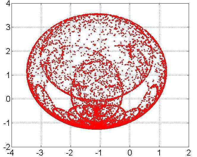
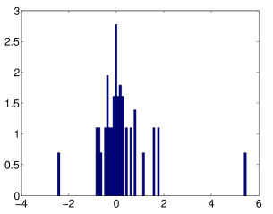
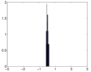
Fig. 1: a) Chaotic attractor for uncontrolled Lorentz system for parameter value of $\alpha=1.25$ and $\beta=0.75$; b) Histogram for the error dynamics between two trajectories for non-erasure probability of $p=0.55$; c) Histogram for the error dynamics between two trajectories for non-erasure probability of $p=0.9$.

3.1 Simulations

For the simulation we choose the parameter value of $(\alpha_{s},\beta_{s})=(1.25,0.75)$. For these parameter values, the local instability at the equilibrium point is dominant over the global instability captured by positive Lyapunov exponents. The stabilizing feedback controller is designed to cancel the nonlinearity of the $x_{n+1}$ dynamics. We assume erasure channel uncertainty model for random variable $\xi_{n}$ with $Prob(\xi_{n}=1)=p$ and $Prob(\xi_{n}=0)=1-p$. Hence, $\mu=p$ and $\sigma^{2}=p(1-p)$ (Refer to Eq. (4)) defines the statistics of the channel uncertainty. The random variable $\gamma_{n}$ is assumed to be zero mean and variance of $0.1^{2}$.

Case $F_{s}\neq F_{m}$: For this case the parameter value for system (12) are chosen to be $(\alpha_{m},\beta_{m})=(2.25,0.29)$. In Figs. 1b and 1c, we show the histogram for the error between the two trajectories for the system (13) for the non-erasure probability of $p=0.55$ and $p=0.9$ respectively. The histogram are obtained by averaging the error dynamics over $3000$ different realization of channel uncertainty random variable $\xi_{n}$.

Case $F_{s}=F_{m}$: For this case the parameter values for both systems (12) & (13) are identical i.e., $(\alpha_{m},\beta_{m})=(\alpha_{s},\beta_{s})=(1.25,0.75)$. For this case system (12)-(13) are in master-slave configuration. The mean square exponentially incremental stability of slave system will imply that the slave system will synchronize its dynamics to that of master system. The synchronization between master and slave system follows from the structure of the system equations (12) and (13). It is clear that one of the trajectories of the slave system is the same as that of master system (i.e., $z_{n}=w_{n}\forall n$, if $z_{0}=w_{0}$). Hence, if the error between any two trajectories of the slave system approaches zero it implies that the slave system is tracking the master system. In Figs. 2a & 2c, we plot the histogram for the error between the two trajectories for system (13). From Figs. 1(b,c) & Figs. 2(a,b), we notice that the wider support for the histogram for the non-erasure probability of $p=0.55$ is indicative of the fact that the the error dynamics have more variance around zero compared to the case of $p=0.9$.

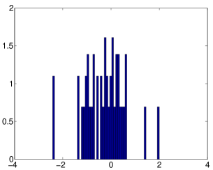
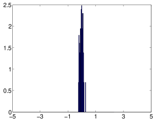
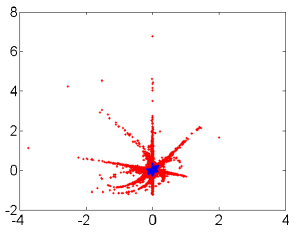
Fig. 2: a) Histogram for the error dynamics between two trajectories for non-erasure probability of $p=0.55$; b) Histogram for the error dynamics between two trajectories for non-erasure probability of $p=0.9$. c) Comparison of two attractors sets for $p=0.65$ (red) and $p=0.9$ (blue).

From the simulation results presented in Figs. (1) (b,c) & (2) (a,b), we conclude that the irrespective of whether $F_{m}=F_{s}$ or $F_{m}\neq F_{s}$, the error dynamics has larger variance for non-erasure probability below $p=0.55$. During this time, the error dynamics is away from zero, loosely speaking, the system trajectories wander on the chaotic attractor. This behavior is sensitive to the presence of additive noise. In particular, additive noise will prevent the error dynamics from converging to zero, thereby manifesting the mean-square instability of the error dynamics in the error trajectories. In Fig. 2c, we plot the attractor set for the slave dynamics (i.e., Eq. (13)) without the coupling from the master system (i.e., $u(w_{n})=0$) for two different values of non-erasure probabilities of $p=0.65$ and $p=0.9$. Comparison of the two attractor sets reveals that attractor set for $p=0.65$ is chaotic, while for $p=0.9$, the attractor is tame with support close to the origin.

The objective of this paper is to provide a rigorous framework that will allow us to distinguish the mean-square stable and unstable behaviors of the error dynamics. In fact, using the main results of this paper in section 5 it can be shown that for the parameter value of $\alpha=1.25$ and $\beta=0.75$ used for the simulation, the critical non-erasure probability below, which the error dynamics for the Lorentz system (13), is mean-square unstable is $p^{*}=0.63$ (or equivalently $\rho^{*}=\frac{\mu^{2}}{\mu^{2}+\sigma^{2}}=0.63$). We will revisit this example with more simulation results later in the simulations Section 6. We will show that for parameter values of $(\alpha_{s},\beta_{s})=(2.25,0.29)$, where the global instability captured by the positive Lyapunov exponent is dominant over the local instability, the limitations and hence the critical non-erasure probability is determined based on global instability.

4 Fundamental limitations for incremental stabilization

The main result of this paper proves the mean-square exponential incremental stabilization of the networked system requires certain minimal QoS from the network. Next, we outline the various steps involved in the proof of this main result.

1. First, we show a necessary condition for the mean-square incremental exponential stability of (7) can be expressed in terms of the mean-square exponential stability of its linearization along the system trajectory (Theorem 4.9).

2. Next, the necessary condition for the mean-square exponential stability for the linearized system is based on the Lyapunov analysis.

3. Finally, the optimal control derived using Lyapunov analysis is used to prove the main results on the mean-square exponential incremental stability.

Theorem 4.9.

Consider the following system dynamics.

$$\eta_{n+1} = \left(\frac{\partial f}{\partial x}(x_{n})+\xi_{n}B\frac{\partial k}{\partial x}(x_{n})\right)\eta_{n}$$ (14)

$$x_{n+1} = f(x_{n}).$$ (15)

Let system (7) be mean-square exponential incremental stable then, the linearized dynamics (14) is mean-square exponential stable, i.e., there exist positive constants $K_{2}<\infty$ and $\beta_{2}<1$, such that,

$$E_{\xi_{0}^{n}}\left[\parallel\eta_{n+1}\parallel^{2}\right]\leq K_{2}\beta_{2}^{n}\parallel\eta_{0}\parallel^{2}\;\;\;\;\forall n\geq 0,$$

for Lebesgue almost all initial conditions $x_{0}\in\mathbb{R}^{N}$ and $x_{0}=0$.

We provide the proof of this Theorem in Appendix 8.

Now, we provide the Lyapunov-based necessary condition for the mean-square exponential stability of a linearized system,

$$\eta_{n+1}=\left(\frac{\partial f}{\partial x}(x_{n})+\xi_{n}B\frac{\partial k}{\partial x}(x_{n})\right)\eta_{n}$$ (16a)

$$x_{n+1}=f(x_{n}).$$ (16b)

Theorem 4.10.

A necessary condition for the linearized system (16b), with controller mapping $k$ satisfying Assumption 2.5, to be mean-square exponentially stable is there exist positive constants, $\alpha_{1}$ and $\alpha_{2}$, and a matrix function of $x$, $P(x)$, such that, $\alpha_{1}I\leq P(x)\leq\alpha_{2}I$ and

$$E_{\xi_{\ell}}\left[{\cal A}^{{}^{\prime}}(x_{\ell},\xi_{\ell})P(x_{\ell+1}){\cal A}(x_{\ell},\xi_{\ell})\right]<P(x_{\ell}),$$ (17)

for almost all with respect to the Lebesgue measure, $x_{0}\in\mathbb{R}^{N}$ and $x_{0}=0$, where ${\cal A}(x_{\ell},\xi_{\ell}):=\frac{\partial f}{\partial x}(x_{\ell})+\xi_{\ell}B\frac{\partial k}{\partial x}(x_{\ell})$ and $x_{\ell+1}=f(x_{\ell})$.

Proof 4.11.

Consider the following construction of $P(x)$.

$$P(x_{\ell}):=\sum_{n=\ell}^{\infty}E_{\xi_{\ell}^{n}}\left[\left(\prod_{k=\ell}^{n}{\cal A}(x_{k},\xi_{k})\right)^{{}^{\prime}}\left(\prod_{k=\ell}^{n}{\cal A}(x_{k},\xi_{k})\right)\right].$$ (18)

From the above construction of $P(x_{\ell})$ and making use of Assumption 2.5 it follows $P(x_{\ell})$ satisfies the inequality (17). Furthermore, since system (16b) is assumed mean-square exponentially stable, we know there exist positive constants $K<\infty$ and $\beta<1$, such that

$$E_{\xi_{0}^{\ell}}\left[\parallel{\cal A}(x_{\ell},\xi_{\ell})\cdots{\cal A}(x_{0},\xi_{0})\parallel^{2}\right]\leq K_{2}\beta_{2}^{\ell}.$$

Hence, there exists a positive constant, $\alpha_{2}$, such that $P(x)\leq\alpha_{2}I$. The lower bound on $P(x)$ and the existence of $\alpha_{1}$ follow from the construction of $P(x)$ and Assumption 2.5.

Definition 4.12 (Matrix Lyapunov function).

We refer to the matrix function $P(x)$ satisfying the necessary condition (17) of Theorem 4.10 as a matrix Lyapunov function.

We now use the matrix Lyapunov function to derive the necessary condition for mean-square exponentail stability.

Theorem 4.13.

The necessary condition for the mean-square exponential stability of a linearized system (16b) is given by

$$A^{{}^{\prime}}(x_{n})Q_{0}(x_{n+1})A(x_{n})-\rho A^{{}^{\prime}}(x_{n})Q_{0}(x_{n+1})B\left(B^{{}^{\prime}}Q_{0}(x_{n+1})B\right)^{-1}B^{{}^{\prime}}Q_{0}(x_{n+1})A(x_{n})<Q_{0}(x_{n}),$$ (19)

for almost all, with respect to the Lebesgue measure initial condition, $x_{0}\in\mathbb{R}^{N}$ and for $x_{0}=0$ and where $\rho=\frac{\mu^{2}}{\mu^{2}+\sigma^{2}}$. The matrix $Q_{0}(x)$ is the solution of the following Riccati-like equation.

$$A^{{}^{\prime}}(x_{n})Q_{0}(x_{n+1})A(x_{n})-A^{{}^{\prime}}(x_{n})Q_{0}(x_{n+1})B\left(I+B^{{}^{\prime}}Q_{0}(x_{n+1})B\right)^{-1}B^{{}^{\prime}}Q_{0}(x_{n+1})A(x_{n})+R(x_{n})$$

$$=Q_{0}(x_{n}),$$ (20)

for some $R(x_{n})\geq 0$, and where $A(x_{n}):=\frac{\partial f}{\partial x}(x_{n})$, $x_{n+1}=f(x_{n})$.

Proof 4.14.

Using the results from Theorem 4.10, we know the necessary condition for the mean-square exponential stability of (16b) can be expressed in terms of the existence of a matrix, Lyapunov function $P(x)$, such that the following inequalities are satisfied, $\alpha_{1}I\leq P(x)\leq\alpha_{2}I$.

$$E_{\xi_{n}}\left[\left(A(x_{n})+\xi_{n}B\frac{\partial k}{\partial x}(x_{n})\right)^{{}^{\prime}}P(x_{n+1})\left(A(x_{n})+\xi_{n}B\frac{\partial k}{\partial x}(x_{n})\right)\right]<P(x_{n}).$$ (21)

Taking expectation w.r.t. $\xi_{n}$, using the fact that $x_{n}$ is independent of $\xi_{n}$, and minimizing the trace of the left-hand side of (21) with respect to $\frac{\partial k}{\partial x}$, we obtain the following expression for the optimal control, $\frac{\partial k}{\partial x}$, in terms of $P(x_{n})$,

$$\frac{\partial k}{\partial x}(x_{n})=-\frac{\mu}{\sigma^{2}+\mu^{2}}\left(B^{{}^{\prime}}P(x_{n+1})B\right)^{-1}B^{{}^{\prime}}P(x_{n+1})A(x_{n}).$$ (22)

Substituting (22) in (21), we obtain the following necessary condition for the mean-square exponential stability,

$$A^{{}^{\prime}}(x_{n})P(x_{n+1})A(x_{n})-\rho A^{{}^{\prime}}(x_{n})P(x_{n+1})B\left(B^{{}^{\prime}}P(x_{n+1})B\right)^{-1}B^{{}^{\prime}}P(x_{n+1})A(x_{n})<P(x_{n}).$$ (23)

where $\rho:=\frac{\mu^{2}}{\mu^{2}+\sigma^{2}}$. It is important to notice the above inequality is independent of scaling, i.e, if $P(x_{n})$ satisfies the above inequality, then $\gamma P(x_{n})$ also satisfies above inequality for any positive constant, $\gamma>0$. By defining $\Delta_{P}:=B^{{}^{\prime}}P(x_{n+1})B\frac{\sigma^{2}}{\mu^{2}}$, we write the above inequality as follows:

$$A^{{}^{\prime}}(x_{n})P(x_{n+1})A(x_{n})-A^{{}^{\prime}}(x_{n})P(x_{n+1})B\left(\Delta_{P}+B^{{}^{\prime}}P(x_{n+1})B\right)^{-1}B^{{}^{\prime}}P(x_{n+1})A(x_{n})<P(x_{n}).$$ (24)

Since $P(x_{n})$ is matrix Lyapunov function, and hence, bounded below, we know there exists a positive constant $\Delta>0$ such that $\Delta I\geq\Delta_{P}$. Hence, (24) implies $P(x_{n})$ satisfies the following inequality,

$$A^{{}^{\prime}}(x_{n})P(x_{n+1})A(x_{n})-A^{{}^{\prime}}(x_{n})P(x_{n+1})B\left(\Delta I+B^{{}^{\prime}}P(x_{n+1})B\right)^{-1}B^{{}^{\prime}}P(x_{n+1})A(x_{n})<P(x_{n}).$$ (25)

Now, since (25) is independent of positive scaling, we obtain from (25)

$$A^{{}^{\prime}}(x_{n})Q_{0}(x_{n+1})A(x_{n})-A^{{}^{\prime}}(x_{n})Q_{0}(x_{n+1})B\left(I+B^{{}^{\prime}}Q_{0}(x_{n+1})B\right)^{-1}B^{{}^{\prime}}Q_{0}(x_{n+1})A(x_{n})<Q_{0}(x_{n}),$$ (26)

where $Q_{0}(x_{n}):=\frac{1}{\Delta}P(x_{n})$. Furthermore (26) implies existence of $R(x_{n})\geq 0$, such that following Riccati-like equality is true

$$A^{{}^{\prime}}(x_{n})Q_{0}(x_{n+1})A(x_{n})-A^{{}^{\prime}}(x_{n})Q_{0}(x_{n+1})B\left(I+B^{{}^{\prime}}Q_{0}(x_{n+1})B\right)^{-1}B^{{}^{\prime}}Q_{0}(x_{n+1})A(x_{n})$$

$$+R(x_{n})=Q_{0}(x_{n}).$$ (27)

The necessary condition (19) then follows from (23). Using the definition, $P(x_{n})=\Delta Q_{0}(x_{n})$. The Riccati-like equation (27) resembles the Riccati equation obtained in the solution of the linear quadratic regulator problem for the linear time varying (LTV) system [37] with the difference that various matrices in (27) are parameterized by a state trajectory $\{x_{n}\}$ of system, $x_{n+1}=f(x_{n})$, instead of time. The matrix function $Q_{0}(x_{n})$ is also bounded both above and below. It follows from the uniformly, completely controllability assumption on pair $(f(x),B)$ (Assumption 2.3).

5 Main results

In this section, we use the result from Theorem 4.13 to derive conditions for mean-square exponential incremental stability under various assumptions on system dynamics.

5.1 Linear system

Theorem 5.15.

For the linear time invariant system (i.e., $f(x)=Ax$) with all eigenvalues having an absolute value greater than one, a necessary condition for the mean-square exponential incremental stability with controller satisfying Assumption 2.5

• for number of control inputs, $1\leq d<N$, is given by

  $$\bar{\rho}^{d}\prod_{k=1}^{N}|\lambda_{k}|^{2}<1.$$ (28)

• for the number of control inputs equal to the number of states, i.e., $d=N$ and $B$ invertible, is given by

  $$\bar{\rho}|\lambda_{max}|^{2}<1,$$ (29)

where, $\bar{\rho}=1-\rho$, $\rho=\frac{\mu^{2}}{\mu^{2}+\sigma^{2}}$, $\lambda_{k}$ for $k=1,\ldots,N$ and $\lambda_{max}$ are the unstable eigenvalues and maximum eigenvalue of matrix $A$, respectively.

Proof 5.16.

For $1\leq d<N$: A necessary condition (19) for mean-square exponential incremental stability from Theorem 4.13 for the special case of a linear time invariant system can be written as,

$$A^{\prime}Q_{0}A-\rho A^{\prime}Q_{0}B(B^{\prime}Q_{0}B)^{-1}B^{\prime}Q_{0}A^{\prime}<Q_{0},$$ (30)

Taking determinants on both sides of the above equation and using the matrix determinant formula, i.e., $\det(I_{N}-\rho B(B^{\prime}Q_{0}B)^{-1}B^{\prime}Q_{0})=\det(I_{d}-\rho(B^{\prime}Q_{0}B)^{-1}B^{\prime}Q_{0}B)$, we obtain

$$\det(A^{\prime}Q_{0})\det(\bar{\rho}I_{d})\det(A)<\det(Q_{0}),$$

where $I_{d}$ in $d\times d$ identity matrix. Simplifying above inequality, we obtain,

$$\bar{\rho}^{d}\det(A)^{2}=\bar{\rho}^{d}\prod_{k=1}^{N}|\lambda_{k}|^{2}.$$ (31)

$N$ input case: For the $N$ input case, matrix $B$ is invertible and a necessary condition for the mean-square exponential incremental stability (19) from Theorem 4.13, and therefore reduces to

$$\bar{\rho}A^{\prime}Q_{0}A<Q_{0}.$$ (32)

A necessary condition for satisfying inequality (32) is given by

$$\bar{\rho}|\lambda_{\max}|^{2}<1.$$

.

Remark 5.17.

Careful examination of the proofs for Theorems 4.9 and 4.13, for the special case of LTI systems, reveals the conditions in Theorem 5.15 are also sufficient for the mean-square exponential incremental stability of the LTI system for $d=1$ and $d=N$. Furthermore, it is not difficult to prove the LTI system is mean-square exponential incremental stable, if and only if, the origin of the system is mean-square exponential stable. Hence, the results of Theorem 5.15 will also provide necessary and sufficient conditions for the mean-square exponential stability of LTI systems over erasure channels for $d=1$ and $d=N$. The results from Theorem 5.15 are consistent and in agreement with the known results for the control of LTI systems over erasure channels for $d=1$ and $d=N$ cases [13].

5.2 Nonlinear system with ergodicity assumption

The main theorem of this section provides a stability condition for nonlinear systems under some ergodicity assumption on system dynamics. In particular, we assume that the uncontrolled system has unique invariant measure (Definition 5.18) and associated positive Lyapunov exponents (Definition 5.19). Lyapunov function-based argument and theorems exists to ensure existence of invariant measure on unbounded state space [39] . Existence of invariant measure guarantee that the system has well defined steady state where the system dynamics eventually settle down. We start with the following definition of physical invariant measure.

Definition 5.18 (Physical invariant measure).

A probability measure $\mu$ defined on $\mathbb{R}^{N}$, is said to be invariant for $x_{n+1}=f(x_{n})$ if $\mu(B)=\mu(f^{-1}(B))$ for all sets $B\in{\cal B}(\mathbb{R}^{N})$ (where $f^{-1}(B)$ is the inverse image of set $B$ and ${\cal B}(\mathbb{R}^{N})$ is the Borel-$\sigma$ algebra on $\mathbb{R}^{N}$). An invariant probability measure is said to be ergodic, if any $f$-invariant set, $A$, i.e., $f^{-1}(A)=A$, has $\mu$ measure equal to one or zero. The ergodic invariant measure is said to be physical, if

$$\lim_{n\to\infty}\frac{1}{n}\sum_{k=0}^{n}\varphi(x_{k})=\int_{\mathbb{R}^{N}}\varphi(x)d\mu(x),$$ (33)

for positive Lebesgue measure set of initial condition $x_{0}\in\mathbb{R}^{N}$ and for all continuous function $\varphi:\mathbb{R}^{N}\to\mathbb{R}$. The physical measure, $\mu$, is said to be unique if (33) holds true for all Lebesgue measure initial condition $x_{0}\in\mathbb{R}^{N}$ and all continuous function $\varphi$.

Definition 5.18 implies for Lebesgue, almost all initial conditions, $x\in\mathbb{R}^{N}$, will distribute themselves, according to the physical measure, $\mu$. A typical chaotic system will have infinitely many ergodic measures, but only one physical measure. Among all the invariant measures the system has, one would expect to see physical measure in the simulation of the dynamical system. Set-oriented numerical methods are available for the computation of a physical measure in dynamical systems [40].

Definition 5.19 (Lyapunov exponents).

For $x_{n+1}=f(x_{n})$, let

$$L(x)=\lim_{n\rightarrow\infty}\left[\left(\prod_{k=0}^{n}\frac{\partial f}{\partial x}(x_{k})\right)^{{}^{\prime}}\left(\prod_{k=0}^{n}\frac{\partial f}{\partial x}(x_{k})\right)\right]^{\frac{1}{2n}},\;\;x_{0}=x.$$ (34)

If $\lambda^{i}_{exp}$ are the eigenvalues of $L(x_{0})$, then the Lyapunov exponents, $\Lambda^{i}_{exp}$, are given by $\Lambda^{i}_{exp}=\log\lambda^{i}_{exp}$ for $i=1,\ldots,N$. The maximum Lyapunov exponent can be obtained as the limit of the following quantity,

$$\Lambda_{exp}(x_{0})=\lim_{n\to\infty}\frac{1}{n}\log\parallel\prod_{k=1}^{n}\frac{\partial f}{\partial x}(x_{k})\parallel,$$ (35)

where $\parallel\cdot\parallel$ is the induced $2-$ norm. Furthermore, if $\det(L(x))\neq 0$ then

$$\lim_{n\to\infty}\frac{1}{n}\log|\det\left(\prod_{k=0}^{n}\frac{\partial f}{\partial x}(x_{k})\right)|=\log\prod_{k=1}^{N}\lambda^{k}_{exp}(x).$$ (36)

Remark 5.20.

The technical condition for the existence of Lyapunov exponents and the limit in (36) is given by the Oseledec multiplicative ergodic theorem [33]. Lyapunov exponents for nonlinear systems are defined with respect to a particular invariant measure. Hence, in general, they will be a function of the initial condition, $x_{0}$. Under the assumption the system has unique physical invariant measure, the Lyapunov exponents and limits in (35) and (36) will be independent of the initial condition, $x_{0}$. The technical conditions required by Oseledec multiplicative ergodic theorem are satisfied by the system map, $f$, in the form of Assumption 1. For a detailed statement of the multiplicative ergodic theorem, we refer readers to [41] (Theorem 10.4) and discussion in section D of [33].

Assumption 5.21.

Assume the system, $x_{n+1}=f(x_{n})$ has a unique physical invariant measure with all its Lyapunov exponents positive.

Remark 5.22.

The assumption on uniqueness of physical invariant measure is not necessary to prove the main results of this section. The main results can be proven under the existence of an ergodic invariant measure (or ergodic decomposition of invariant measure) guaranteed to exist following Remark 5.20. However, the assumption of a unique physical measure allows us to prove the main results that are independent of the initial conditions. Without the uniqueness assumption, the main result of this section will be a function of the initial condition, $x$. The assumption of all Lyapunov exponents positive is similar to the assumption made for the case of LTI systems all eigenvalues are positive. The physical measure with a positive Lyapunov exponent implies the existence of an attractor set with chaotic dynamics. Furthermore, the assumption of all Lyapunov exponent positive is a technical assumption and is made for the simplicity of presentation. This assumption can be relaxed using the technique of tempered transformation [36], which allows one to decompose the state space into directions of positive and negative exponents.

Theorem 5.23.

Consider system (7) with system mapping, $f$, satisfying Assumptions 1, 2.3, and 5.21. Then, a necessary condition for the mean-square exponential incremental stability with controller mapping satisfying Assumption 2.5

• for the number of control inputs $1\leq d<N$ is given by

  $$\bar{\rho}^{d}\max\left(\prod_{k=1}^{N}\left(\lambda^{k}_{\exp}\right)^{2},\prod_{k=1}^{N}\left(|\lambda^{k}_{0}|\right)^{2}\right)<1,$$ (37)

  where $\bar{\rho}=1-\rho$, $\lambda^{k}_{exp}=\exp^{\Lambda^{k}_{exp}}$ and $\Lambda^{k}_{exp}>0$ is the $k^{th}$ positive Lyapunov exponent of the system, $x_{n+1}=f(x_{n})$, and $\lambda_{0}^{k}$ are the unstable eigenvalues of the Jacobian, $\frac{\partial f}{\partial x}(0)$, at the origin.

• the $N$ input case is given by

  $$\bar{\rho}\max\left((\lambda_{exp}^{1})^{2},|\lambda_{max}|^{2}\right)<1,$$ (38)

  where $\lambda^{1}_{exp}=\exp^{\Lambda^{1}_{exp}}$ and $\Lambda^{1}_{exp}>0$ is the maximum Lyapunov exponent of the system, $x_{n+1}=f(x_{n})$, and $\lambda_{max}$ is the maximum eigenvalue of the Jacobian $\frac{\partial f}{\partial x}(0)$.

Proof 5.24.

For $1\leq d<N$: Using the results from Theorem 4.13, a necessary condition for mean-square exponential incremental stability is given by,

$$A^{\prime}(x_{n})Q_{0}(x_{n+1})A(x_{n})-\rho A^{\prime}(x_{n})Q_{0}(x_{n+1})B(B^{\prime}Q_{0}(x_{n+1})B)^{-1}B^{\prime}Q_{0}(x_{n+1})A(x_{n})<Q_{0}(x_{n}).$$ (39)

$Q_{0}(x)$ satisfies the following Riccati-like equation,

$$A^{\prime}(x_{n})Q_{0}(x_{n+1})A(x_{n})-A^{\prime}(x_{n})Q_{0}(x_{n+1})B(I+B^{\prime}Q_{0}(x_{n+1})B)^{-1}B^{\prime}Q_{0}(x_{n+1})A(x_{n})$$

$$+R(x_{n})=Q_{0}(x_{n}),$$ (40)

where $x_{n+1}=f(x_{n})$ and $A(x_{n}):=\frac{\partial f}{\partial x}(x_{n})$. Taking determinants on both the sides of (39) and using the matrix determinant formula, i.e., $\det(I_{N}-\rho B(B^{\prime}Q_{0}(x_{n+1})B)^{-1}B^{\prime}Q_{0}(x_{n+1}))=\det(I_{d}-\rho(B^{\prime}Q_{0}(x_{n+1})B)^{-1}B^{\prime}Q_{0}(x_{n+1})B)$, we obtain

$$\bar{\rho}^{d}\det(A^{2}(x_{n}))\det(Q_{0}(x_{n+1})Q^{-1}_{0}(x_{n}))<1.$$ (41)

The above necessary condition holds true for all initial conditions, $x_{n}$. Hence, we can evaluate the above condition along the system trajectory, $x_{n+1}=f(x_{n})$. We obtain

$$\bar{\rho}^{dn}\det(Q_{0}(x_{n+1}))\prod_{k=0}^{n}\det(A^{2}(x_{k}))\det(Q^{-1}_{0}(x_{0}))<1.$$ (42)

Taking the logarithm and average with respect to $n$ and in the limit as $n\to\infty$ of the above expression, we obtain

$$\log\bar{\rho}^{d}+\lim_{n\to\infty}\frac{1}{n}\log\left(\det(Q_{0}(x_{n+1}))\prod_{k=0}^{n}\det(A^{2}(x_{k}))\det(Q^{-1}_{0}(x_{0}))\right)<0.$$

Now, using the fact that $Q_{0}(x)$ is bounded above and below, and using equality (36) from Definition 5.18, we obtain the following necessary condition for stability,

$$\bar{\rho}^{d}\prod_{k=1}^{N}(\lambda_{exp}^{k})^{2}<1.$$ (43)

Similarly, if we evaluate the necessary condition (41) at the equilibrium point, $x=0$, we obtain

$$\bar{\rho}^{d}\prod_{k=1}^{N}(|\lambda_{0}^{k}|)^{2}<1.$$ (44)

Combining (43) and (44), we obtain the required necessary condition (37) for stability.
$N$ input case: With the $N$ input case, the matrix, $B$, is invertible. The necessary condition (19) for mean-square exponential incremental stability reduces to

$$\bar{\rho}A^{\prime}(x_{n})Q(x_{n+1})A(x_{n})<Q(x_{n}).$$ (45)

Since $Q(x_{n})$ is both bounded above and below, there exists an invertible matrix $T(x_{n})$, such that $Q(x_{n})=T^{\prime}(x_{n})T(x_{n})$. The necessary condition (45) can be written as

$$\bar{\rho}\hat{A}^{\prime}(x_{n})\hat{A}(x_{n})<I,$$

where $\hat{A}(x_{n}):=T(x_{n+1})A(x_{n})T^{-1}(x_{n})$. Since the above inequality holds true for almost all initial conditions, we can evaluate the inequality along the trajectory of the system $x_{n+1}=f(x_{n})$. We obtain

$$\bar{\rho}^{n}\hat{A}^{\prime}(x_{0})\hat{A}^{\prime}(x_{1})\cdots\hat{A}^{\prime}(x_{n-1})\hat{A}(x_{n-1})\cdots\hat{A}(x_{1})\hat{A}(x_{0})<I,$$

which is equivalent to

$$\bar{\rho}^{n}(T^{-1}(x_{0}))^{{}^{\prime}}A^{\prime}(x_{0})A(x_{1})\cdots A(x_{n-1})Q(x_{n})A(x_{n-1})\cdots A(x_{1})A(x_{0})T^{-1}(x_{0})<I.$$

Again, using the fact $Q(x)$ is bounded above and below, the above inequality implies the following necessary condition for stability,

$$\log\bar{\rho}+\lim_{n\to\infty}\frac{1}{n}\log\parallel\prod_{k=0}^{n}A(x_{k})\parallel^{2}<0.$$

Using equality (35) from Definition 5.18, we obtain the following necessary condition for stability

$$\bar{\rho}(\lambda^{1}_{exp})^{2}<1,$$ (46)

where $\lambda_{exp}^{1}$ is the maximum Lyapunov exponent of the system, $x_{n+1}=f(x_{n})$. Similarly, evaluating the necessary conditions for stability at the equilibrium point, $x=0$, we obtain

$$\bar{\rho}|\lambda_{max}|^{2}<1.$$ (47)

Combining (46) and (47), we obtain the desired necessary condition (38) for stability of the $N$ input case.

The results of Theorem 5.23 can be viewed as the generalization of the results from Theorem 5.15 for LTI systems, where Lyapunov exponents emerge as the natural generalization of linear system eigenvalues to nonlinear systems.

5.3 Sufficient condition for stability

Theorem 5.25 provides sufficient condition for stability.

Theorem 5.25.

System (7), satisfying Assumptions 1 and 2.3, is mean-square exponential incrementally stable for all values of non-erasure probability, $p$, that satisfies

$$\frac{\partial f(x)}{\partial x}^{{}^{\prime}}\left(P-pPB(B^{\prime}PB)^{-1}B^{\prime}P\right)\frac{\partial f(x)}{\partial x}<P,$$ (48)

for almost all with respect to the Lebesgue measure, $x\in X$ and for $x=0$, where matrix $P>0$ satisfies the following Riccati equation,

$$A^{\prime}PA-A^{\prime}PB(I+B^{\prime}PB)B^{\prime}PA=P,$$

with $A=\frac{\partial f}{\partial x}(0)$.

Proof 5.26.

Let $k(x)=-(B^{\prime}PB)^{-1}B^{\prime}Pf(x)$ be the feedback control input. With this input, we obtain $x_{n+1}=(I-\xi_{n}B(B^{\prime}PB)^{-1}B^{\prime}P)f(x_{n})$. Consider any two points, $x_{0}$ and $y_{0}$, in $X$ and the curve joining these two points given by $z_{0}(\alpha)=\alpha x_{0}+(1-\alpha)y_{0}$ with $\alpha\in[0,1]$. The dynamical evolution of this curve, $z_{0}(\alpha)$, is given by $z_{n+1}(\alpha)=(I-\xi_{n}B(B^{\prime}PB)^{-1}B^{\prime}P)f(z_{n}(\alpha))$. Define a new variable, $\zeta_{n}=\frac{\partial z_{n}}{\partial\alpha}$. Hence, we obtain

$$\zeta_{n+1}=\frac{\partial z_{n+1}}{\partial\alpha}=(I-\xi_{n}B(B^{\prime}PB)^{-1}B^{\prime}P)\frac{\partial f}{\partial z}(z_{n})\zeta_{n}.$$

The length of the curve, $z_{0}(\alpha)$, after $n$ iterations is given by $\int_{0}^{1}\parallel\zeta_{n}\parallel d\alpha$. Defining new coordinates, $\rho_{n}=P^{\frac{1}{2}}\zeta_{n}=T\zeta_{n}$, we obtain

$$\rho_{n+1}=T(I-\xi_{n}B(B^{\prime}PB)^{-1}B^{\prime}P)\frac{\partial f}{\partial z}(z_{n})T^{-1}\rho_{n}.$$

Using (48), we obtain

$$E_{\xi_{0}^{n}}\left[\parallel\rho_{n+1}\parallel^{2}\right]\leq\beta^{n}\parallel\rho_{0}\parallel^{2}$$

for some $\beta<1$. Using the fact there exist positive constants, $\tau_{1}$ and $\tau_{2}$, such that $\tau_{1}I\leq P\leq\tau_{2}I$, we obtain

$$E_{\xi_{0}^{n}}\left[\parallel\zeta_{n+1}\parallel^{2}\right]\leq\beta^{n}\frac{\tau_{2}}{\tau_{1}}\parallel\zeta_{0}\parallel^{2}=K\beta^{n}\parallel\zeta_{0}\parallel^{2}.$$

We have

$$E_{\xi_{0}^{n}}\left[\parallel x_{n+1}-y_{n+1}\parallel^{2}\right]\leq\int_{0}^{1}E_{\xi_{0}}^{n}[\parallel\zeta_{n+1}\parallel^{2}]d\alpha\leq K\beta^{n}\parallel x_{0}-y_{0}\parallel^{2}.$$

6 Example

In this section, we continue with the discussion on the synchronization in discrete Lorentz system started in Section 3. As mentioned previously, there are two competing instabilities the controller needs to work against to stabilize the unstable equilibrium at the origin. The parameter values, $\alpha$ and $\beta$, can be chosen so the instability at the equilibrium point $(0,0)$ is larger or smaller than the average instability on the attractor set captured by the Lyapunov exponents. In particular, for a parameter value of $\alpha=1.25$ and $\beta=0.75$, the eigenvalues for the linearization at the origin are $\lambda_{1}=1.28$ and $\lambda_{2}=1.28$ with the product equal to $1.65$. The positive Lyapunov exponent for these parameter values is equal to $\Lambda_{exp}=.34$. Hence, $\lambda_{exp}=\exp{0.34}=1.40<\lambda_{1}\lambda_{2}=1.65$. So, the critical erasure probability is computed, based on the unstable eigenvalues, and equals $p_{eig}^{*}=1-\frac{1}{\lambda_{1}^{2}\lambda_{2}^{2}}=0.63$.

For the parameter values, $\alpha=2.25$ and $\beta=0.29$, the product of the unstable eigenvalues at the origin equals $\lambda_{1}\lambda_{2}=1.08$ and the exponential of the positive Lyapunov exponent is equal to $\lambda_{exp}=1.13$. This leads to the critical non-erasure probability, based on the positive Lyapunov exponent equal to $p^{*}_{lya}=1-\frac{1}{\lambda_{exp}^{2}}=0.21$. The critical non-erasure probability, based on the unstable eigenvalues, is $p_{eig}=0.14$. The controller $k(x)$ is designed to cancel the nonlinearity (i.e., $u_{n}=k(x_{n})=-[(1+\alpha\beta)(x_{n}+\sqrt{\alpha})-\beta(x_{n}+\sqrt{\alpha})(y_{n}+\alpha)-\sqrt{\alpha}]$. In Fig. 3a, we show the attractor set for the uncontrolled system for the parameter value of $\alpha=2.25$ and $\beta=0.29$. The attractor set for the parameter value of $\alpha=1.25$ and $\beta=0.75$ is already shown in Fig. 1a. The attractor set in Figs. 1a and 3a correspond to the physical measure of the Lorentz system for two different sets of parameter values.

6.1 Simulations

In Fig. 3, we show the simulation results for the parameter value of $\alpha=2.25$ and $\beta=0.29$, corresponding to the case where the instability due to the Lyapunov exponent is dominant over the eigenvalues. In Figs. 3b and 3c, we show the histogram for the state error plot between the two trajectories of the system (13) for non-erasure probability of $p=0.15(<0.21=p^{*})$ and for $p=0.35$ respectively. This simulation results in Fig. 3 are obtained for the case where $F_{s}\neq F_{m}$. Similarly, in Figs. 4a and 4b, we show the histogram of the error plots for the case of $F_{s}=F_{m}$.

Comparing Fig.3a with Fig. 3b and Fig. 4a with 4b, we notice the error dynamics show larger fluctuation around zero for non-erasure probability below the critical value of $p^{*}$. It is important to emphasize that the non-erasure probability, $p=0.15$, satisfies $p_{eig}=0.14<0.15<0.21=p^{*}_{lya}$. Hence, although the system has overcome local instability due to eigenvalues, the global instability of the attractor set is still a limiting factor for stabilization. This is further evident from comparing the two attractor sets obtained for the $p=0.15$ and $p=0.28$ in Fig. 4c. These two attractor sets are obtained by simulating the system Eq. (13) without the coupling from system (12). From this plot, we see that the attractor set for $p=0.15$ (in red) is chaotic, but for $p=0.28$, the attractor set (in blue) is concentrated around the origin. Finally, in Figs. 5a and 5b, we show the plot for the linearized error covariance for the parameter values of $(\alpha=1.25,\beta=0.75)$, and $(\alpha=2.25,\beta=0.29)$ respectively. From these plots, we clearly see that the covariance for parameter values of $(\alpha=1.25,\beta=0.75)$ and $(\alpha=2.25,\beta=0.29)$ become unbounded for non-erasure probability of $p^{*}=0.21$ and $p^{*}=0.63$, respectively, as predicted by the main result of this paper. The predicted value of critical non-erasure probability of $p^{*}=0.63$ is in agreement with the simulation results presented in section 3.

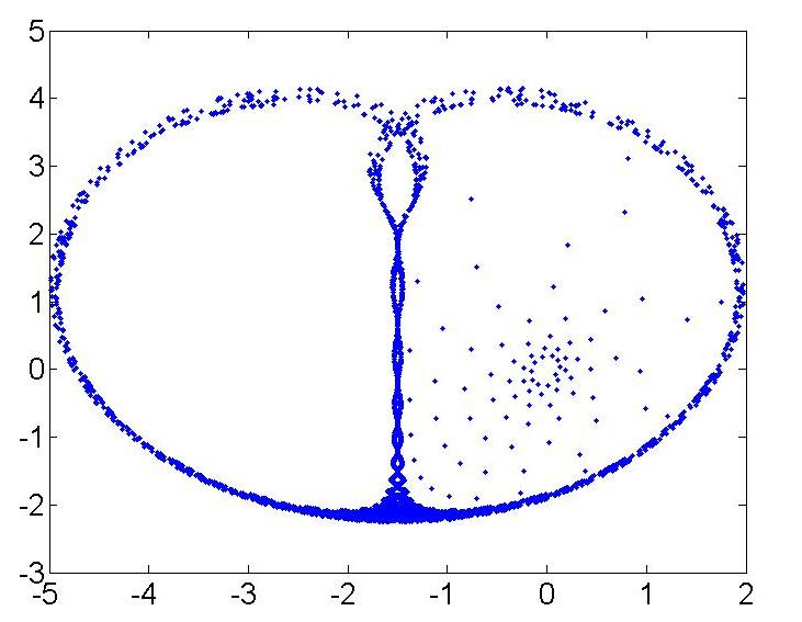
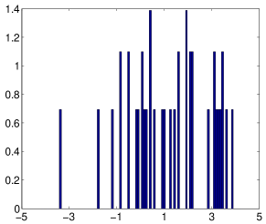
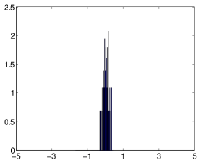
Fig. 3: a) Chaotic attractor for parameters $\alpha=2.25,\beta=0.29$); b) Histogram for the error dynamics between two trajectories for non-erasure probability of $p=0.15<p^{*}=0.21$; c) Histogram for the error dynamics between two trajectories for non-erasure probability of $p=0.3$.

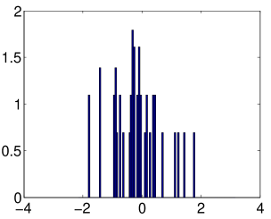
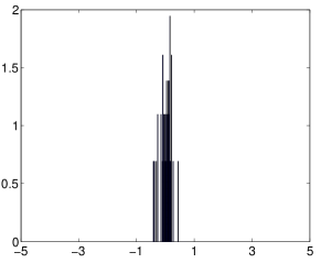
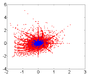
Fig. 4: a) Histogram for the error dynamics between two trajectories for non-erasure probability of $p=0.15$; b) Histogram for the error dynamics between two trajectories for non-erasure probability of $p=0.3$; c) Comparison of two attractor sets for $p=0.15$ (red) and $p=0.28$ (blue);

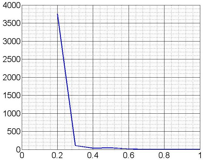
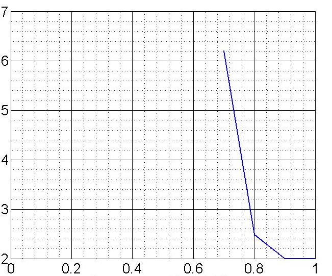
Fig. 5: a) Trace of the linearized covariance vs non-erasure probability $p$ for $(\alpha,\beta)=(2.25,0.29)$; b) Trace of the linearized covariance vs non-erasure probability $p$ for $(\alpha,\beta)=(1.25,0.75)$.

7 Conclusions

In this paper, we considered the problem of incremental stabilization of a class of nonlinear systems by state feedback controller, when the actuation command may be lost on a communication link with certain probability. The stochastic notion of mean-square exponential stability is adopted to study the incremental stabilization problem over an uncertain communication link. One of the important features of our main results is its global nature away from equilibrium and the emergence of the open-loop Lyapunov exponents as the natural generalization of the linear system eigenvalues in capturing the system limitations. Our results are quite encouraging and our novel approach, based on ergodic theory of dynamical system, is amenable to various extensions.

8 Appendix

Proof of Theorem 2.8

Proof 8.27.

From the definition of mean square exponential incremental stability of system (7) and using the fact that $f(0)=k(0)=0$ (Assumption 1 and 2.5) it follows that system

$$x_{n+1}=f(x_{n})+\xi_{n}Bk(x_{n})=:T(x_{n},\xi_{n}).$$ (49)

is mean square exponentially stable i.e., there exist positive constants $\bar{K}_{1}<\infty$ and $\bar{\beta}_{1}<1$ such that

$$E_{\xi_{0}^{n}}[\parallel x_{n+1}\parallel^{2}]\leq\bar{K}_{1}\bar{\beta}_{1}^{n}\parallel x_{0}\parallel^{2}.$$ (50)

Furthermore, following Holder’s Inequality we also obtain

$$E_{\xi_{0}^{n}}[\parallel x_{n+1}\parallel]\leq\left(E_{\xi_{0}^{n}}[\parallel x_{n+1}\parallel^{2}]\right)^{\frac{1}{2}}\leq\left(\bar{K}_{1}\bar{\beta}_{1}^{n}\parallel x_{0}\parallel^{2}\right)^{\frac{1}{2}}=\bar{K}_{1}^{\frac{1}{2}}\bar{\beta}_{1}^{\frac{n}{2}}\parallel x_{0}\parallel.$$ (51)

The mean square exponential stability of (49) implies existence of Lyapunov function, $V(x)$, satisfying following conditions

$$c_{1}\parallel x_{n}\parallel^{2}\leq V(x_{n})\leq c_{2}\parallel x_{n}\parallel^{2},\;\;E_{\xi_{n}}[V(T(x_{n},\xi_{n}))]\leq\alpha V(x_{n})$$

$$\parallel\frac{\partial V}{\partial x}(x_{n})\parallel\leq c_{3}\parallel x_{n}\parallel,$$

where, $c_{1}=1,c_{2},c_{3}$ are positive constants and $\alpha<1$. This can be proved as follows. Consider the following construction of Lyapunov function.

$$V(x_{n})=\parallel x_{n}\parallel^{2}+\sum_{k=n+1}^{\infty}E_{\xi_{n}^{k-1}}[\parallel x_{k}\parallel^{2}]\implies V(x_{n+1})=\parallel x_{n+1}\parallel^{2}+\sum_{k=n+2}^{\infty}E_{\xi_{n+1}^{k-1}}[\parallel x_{k}\parallel^{2}]$$

where $x_{n+1}=T(x_{n},\xi_{n})$. From the construction of $V$, it is clear that $V(x_{n})\geq\parallel x_{n}\parallel^{2}$, hence $c_{1}=1$. The upper bound follows from the mean square exponentially stability of (49) as follows

$$V(x_{n})=\parallel x_{n}\parallel^{2}+\sum_{k=n+1}^{\infty}E_{\xi_{n}^{k-1}}[\parallel x_{k}\parallel^{2}]\leq\parallel x_{n}\parallel^{2}+\sum_{k=n+1}^{\infty}\bar{K}_{1}\bar{\beta}_{1}^{k-1-n}\parallel x_{n}\parallel^{2}\leq\parallel x_{n}\parallel^{2}c_{2},$$

where $c_{2}:=\bar{K}_{1}(1+\frac{1}{1-\bar{\beta}_{1}})>1$. From the construction of $V$, it follows that

$$E_{\xi_{n}}[V(x_{n+1})]=V(x_{n})-\parallel x_{n}\parallel^{2}\leq(1-\frac{1}{c_{2}})V(x_{n})=\alpha V(x_{n})$$

since $c_{2}>1$, $(1-\frac{1}{c_{2}})=:\alpha<1$. We next prove the bound on the derivative of Lyapunov function $V$. Towards this goal we make use of the Assumptions 1 and 2.5 providing uniform bounds for the Jacobian of system mapping, $f$, and feedback controller, $k$. We have

$$\left|\frac{\partial T}{\partial x}(x,\xi)\right|=\left|\frac{\partial f}{\partial x}(x)+\xi B\frac{\partial k}{\partial x}(x)\right|\leq L(1+|\xi|)$$

where $L$ is the assumed uniform bound on the Jacobian of $f$ and $Bk$ i.e., $\max\{\parallel\frac{\partial f}{\partial x}\parallel,\parallel B\frac{\partial k}{\partial x}\}\leq L$. We introduce following notation

$$x_{2}=T(T(x_{0},\xi_{0}),\xi_{1})=:T^{2}(x_{0},\xi_{0}^{1}),\;\;{\rm hence},\;\;x_{k}=T^{k}(x_{0},\xi_{0}^{k-1})$$

We now have

$$\frac{\partial V}{\partial x}(x)=2x+2\sum_{k=1}^{\infty}E_{\xi_{0}^{k-1}}\left[\left[\frac{\partial T}{\partial x}\left(T^{k-1}(x,\xi_{0}^{k-2}),\xi_{k-1}\right)\right]^{\top}T^{k}(x,\xi_{0}^{k-1})\right].$$

Hence,

$$\parallel\frac{\partial V}{\partial x}(x)\parallel\leq 2\parallel x\parallel+2L\sum_{k=1}^{\infty}E_{\xi_{0}^{k-1}}\left[(1+|\xi_{k-1}|)\parallel x_{k}\parallel\right].$$ (52)

Now we use following using Holder’s inequality

$$E_{\xi_{0}^{k-1}}\left[|\xi_{k-1}|\parallel x_{k}\parallel\right]\leq\left(E_{\xi_{0}^{k-1}}\left[|\xi_{k-1}|^{2}\right]\right)^{\frac{1}{2}}\left(E_{\xi_{0}^{k-1}}\left[\parallel x_{k}\parallel^{2}\right]\right)^{\frac{1}{2}}=(\sigma^{2}+\mu^{2})^{\frac{1}{2}}\left(E_{\xi_{0}^{k-1}}\left[\parallel x_{k}\parallel^{2}\right]\right)^{\frac{1}{2}}$$ (53)

Combining inequalities (50), (51) and (53), we obtain

$$\parallel\frac{\partial V}{\partial x}(x)\parallel\leq 2\parallel x\parallel+2L\sum_{k=1}^{\infty}E_{\xi_{0}^{k-1}}\left[\parallel x_{k}\parallel\right]+2L(\sigma^{2}+\mu^{2})^{\frac{1}{2}}\sum_{k=1}^{\infty}\left(E_{\xi_{0}^{k-1}}\left[\parallel x_{k}\parallel^{2}\right]\right)^{\frac{1}{2}}$$

$$\parallel\frac{\partial V}{\partial x}(x)\parallel\leq\left(2+2L\sum_{k=1}^{\infty}\bar{K}_{1}^{\frac{1}{2}}\bar{\beta}_{1}^{\frac{k-1}{2}}+2L(\sigma^{2}+\mu^{2})^{\frac{1}{2}}\sum_{k=1}^{\infty}\bar{K}_{1}^{\frac{1}{2}}\bar{\beta}_{1}^{\frac{k-1}{2}}\right)\parallel x\parallel=:c_{3}\parallel x\parallel$$

We now consider system

$$x_{n+1}=T(x_{n},\xi_{n})+\gamma_{n}$$

in the rest of the proof. Using the Lyapunov function, following inequality holds true for the above system

$$E_{\xi_{0}^{n}\gamma_{0}^{n}}[\parallel x_{n+1}\parallel^{2}]\leq\frac{1}{c_{1}}E_{\xi_{0}^{n}\gamma_{0}^{n}}[V(x_{n+1})]=\frac{1}{c_{1}}E_{\xi_{0}^{n}\gamma_{0}^{n}}[V(T(x_{n},\xi_{n})+\gamma_{n})].$$

We now apply Mean Value Theorem to expand, $V$, as follows

$$V(T(x_{n},\xi_{n})+\gamma_{n})=V(T(x_{n},\xi_{n}))+\frac{\partial V}{\partial x}(T(x_{n},\xi_{n})+c_{n}\gamma_{n})\gamma_{n}$$

for some $c_{n}\in[0,1]$, which in general function of $\gamma_{n}$. Using the fact that $c_{n}$ is bounded by one and using Holder’s inequality we obtain

$$E_{\xi_{n}\gamma_{n}}[V(T(x_{n},\xi_{n})+\gamma_{n})] \leq E_{\xi_{n}}[V(T(x_{n},\xi_{n}))]+c_{3}E_{\xi_{n}\gamma_{n}}[\parallel T(x_{n},\xi_{n})\parallel\parallel\gamma_{n}\parallel]+c_{3}E_{\gamma_{n}}[\parallel\gamma_{n}\parallel^{2}]$$ (54)

$$\leq E_{\xi_{n}}[V(T(x_{n},\xi_{n}))]+c_{3}C^{\frac{1}{2}}\left(E_{\xi_{n}}[\parallel T(x_{n},\xi_{n})\parallel^{2}]\right)^{\frac{1}{2}}+c_{3}C$$

Now using the fact that $\parallel x\parallel^{2}\leq V(x_{n}),E_{\xi_{n}}[V(T(x_{n},\xi_{n}))]\leq\alpha V(x_{n})$, we obtain

$$E_{\xi_{n}\gamma_{n}}[V(T(x_{n},\xi_{n})+\gamma_{n})]\leq\alpha V(x_{n})+b_{1}\left(V(x_{n})\right)^{\frac{1}{2}}+\bar{Q}$$

where $b_{1}:=c_{3}C^{\frac{1}{2}}\alpha^{\frac{1}{2}}$ and $\bar{Q}:=c_{3}C$. Now choose $\alpha_{0}<1-\alpha$. Using inequality of arithmetic and geometric means (AM-GM) we obtain

$$\left(\frac{b_{1}^{2}\alpha_{0}}{\alpha_{0}}V(x_{n})\right)^{\frac{1}{2}}\leq\frac{\alpha_{0}}{2}V(x_{n})+\frac{b_{1}^{2}}{2\alpha_{0}}$$

Using the AM-GM inequality, we write

$$E_{\xi_{n}\gamma_{n}}[V(T(x_{n},\xi_{n})+\gamma_{n})]\leq(\alpha+\frac{\alpha_{0}}{2})V(x_{n})+\frac{b_{1}^{2}}{2\alpha_{0}}+\bar{Q}$$

Since $\alpha_{0}<1-\alpha$, we have $\beta_{2}:=\alpha+\frac{\alpha_{0}}{2}<1$ and defining $Q:=\bar{Q}+\frac{b_{1}^{2}}{2\alpha_{0}}<\infty$, we obtain

$$E_{\xi_{n}\gamma_{n}}[V(T(x_{n},\xi_{n})+\gamma_{n})]\leq\beta_{2}V(x_{n})+Q$$

Taking expectation over the sequence $\{\xi_{n-1},\ldots,\xi_{0}\}$ and $\{\gamma_{n-1},\ldots,\gamma_{0}\}$ and using induction, we obtain

$$E_{\xi_{0}^{n},\gamma_{0}^{n}}[\parallel x_{n+1}\parallel^{2}] \leq E_{\xi_{0}^{n}\gamma_{0}^{n}}[V(T(x_{n},\xi_{n})+\gamma_{n})]\leq\beta_{2}^{n+1}V(x_{0})+Q\sum_{k=0}^{n}\beta_{2}^{k}$$ (55)

$$\leq \beta_{2}^{n}c_{2}\parallel x_{0}\parallel^{2}+\frac{Q}{1-\beta_{2}}$$

Proof of Theorem 4.9.

Proof 8.28.

From the mean square exponential incremental stability of system (7) we know that following is true

$$x_{n+1}=f(x_{n})+\xi_{n}Bk(x_{n})+\xi_{n}Bw_{n}$$ (56)

$$E_{\xi_{0}^{n}}[\parallel x_{n+1}-y_{n+1}\parallel^{2}]\leq K_{1}\beta_{1}^{n}\parallel x_{0}-y_{0}\parallel^{2}$$

for $x_{0},y_{0}\in\mathbb{R}^{N}$ and for some positive constants $K_{1}$ and $\beta_{1}<1$. Since, $w_{n}$ is exogenous input, let $w_{n}=-k(z_{n})$ in (56) with $z_{n}$ evolving according to the dynamics $z_{n+1}=f(z_{n})$. Hence, we have

$$z_{n+1} = f(z_{n})$$ (57)

$$x_{n+1} = f(x_{n})+\xi_{n}Bk(x_{n})-\xi_{n}Bk(z_{n}).$$ (58)

Since system (58) is mean square exponentially incrementally stable, hence all the trajectories of system (58) will converge to each other. One particular trajectory of the system (58), say $\bar{x}_{n}$, is obtained by taking the initial condition $\bar{x}_{0}=z_{0}$, which gives us $\bar{x}_{n}=z_{n}$ for all $n\geq 0$. Hence, from the mean-square exponential incremental stability of system (58), it follows

$$E_{\xi_{0}^{n}}\left[\parallel x_{n+1}-z_{n+1}\parallel^{2}\right]=E_{\xi_{0}^{n}}\left[\parallel x_{n+1}-\bar{x}_{n+1}\parallel^{2}\right]\leq K_{1}\beta_{1}^{n}\parallel x_{0}-\bar{x}_{0}\parallel^{2}=K\beta^{n}\parallel x_{0}-z_{0}\parallel^{2},$$ (59)

for $\forall n\geq 0$ and Lebesgue almost all initial conditions, $x_{0},z_{0}\in\mathbb{R}^{N}$ and, in particular, for $z_{0}=0$. Using (57) and (58), we obtain

$$e_{n+1}:=z_{n+1}-x_{n+1}=(f(z_{n})+\xi_{n}Bk(z_{n}))-(f(x_{n})+\xi_{n}Bk(x_{n})).$$ (60)

Define ${\cal A}(z_{n},\xi_{n}):=\frac{\partial f}{\partial z}(z_{n})+\xi_{n}B\frac{\partial k}{\partial z}(z_{n})$. Then, using (60) and the Mean value theorem for a vector valued function , we obtain

$$e_{n+1} = \int_{0}^{1}{\cal A}(z_{n}-se_{n},\xi_{n})dse_{n}=\left(\int_{0}^{1}{\cal A}(z_{n}-se_{n},\xi_{n})ds\right)\cdots\left(\int_{0}^{1}{\cal A}(z_{0}-se_{0},\xi_{0})ds\right)e_{0}$$ (61)

$$=: \prod_{k=0}^{n}\left(\int_{0}^{1}{\cal A}(z_{k}-se_{k},\xi_{k})ds\right)e_{0}.$$

Note, $e_{n}$ is a function of $e_{0},x_{0}$, and the random sequence $\xi_{0}^{n-1}$. Hence, we define ${\cal B}_{n}(z_{0},e_{0},\xi_{0}^{n-1}):=\int_{0}^{1}{\cal A}(z_{n}-se_{n},\xi_{n})ds$ and ${\cal B}_{0}^{n}(z_{0},e_{0},\xi_{0}^{n-1}):=\prod_{k=0}^{n}\int_{0}^{1}{\cal A}(z_{k}-se_{k},\xi_{k})ds$. Using the above definitions and mean-square exponential incremental stability property and (59), we know there exist positive constants, $K_{1}<\infty$ and $\beta_{1}<1$, such that

$$E_{\xi_{0}^{n}}\left[\parallel e_{n+1}\parallel^{2}\right]=e_{0}^{\prime}E_{\xi_{0}^{n}}\left[{\cal B}_{0}^{n}(z_{0},e_{0},\xi_{0}^{n})^{\prime}{\cal B}_{0}^{n}(z_{0},e_{0},\xi_{0}^{n})\right]e_{0}\leq K_{1}\beta_{1}^{n}e_{0}^{\prime}e_{0}.$$

Note that the above inequality holds true for any positive scaling of $e_{0}$. Let $\alpha_{\ell}$ be the scaling of $e_{0}$, where $\{\alpha_{\ell}\}$ be the sequence such that $\lim_{\ell\to\infty}\alpha_{\ell}=0$. We then have

$$e_{0}^{\prime}E_{\xi_{0}^{n}}\left[{\cal B}_{0}^{n}(z_{0},\alpha_{\ell}e_{0},\xi_{0}^{n})^{\prime}{\cal B}_{0}^{n}(z_{0},\alpha_{\ell}e_{0},\xi_{0}^{n})\right]e_{0}\leq K_{1}\beta_{1}^{n}e_{0}^{\prime}e_{0}.$$ (62)

Let ${\cal B}_{0}^{n}(z_{0},e_{o},\xi_{0}^{n})_{ij}$ denote the $i^{th}$ row and $j^{th}$ column entry of the matrix ${\cal B}_{0}^{n}(z_{0},e_{0},\xi_{0}^{n})$. From Assumptions 1 and 2.5, we know that both $\frac{\partial f}{\partial z}$ and $\frac{\partial k}{\partial z}$ are uniformly bounded. Hence, for any fixed $n$, we apply Dominated Convergence Theorem to the function ${\cal A}_{ij}(z_{n}-\alpha_{\ell}e_{n},\xi_{0}^{n})$. ${\cal A}_{ij}$ denotes the $ij$ entry of matrix ${\cal A}$. We obtain

$$\lim_{\ell\to\infty}{\cal B}_{n}(z_{0},\alpha_{\ell}e_{0},\xi_{0}^{n})_{ij}=\lim_{\ell\to\infty}\int_{0}^{1}{\cal A}_{ij}(z_{n}-s\alpha_{\ell}e_{n},\xi_{0}^{n})ds={\cal A}_{ij}(z_{n},\xi_{0}^{n})={\cal B}_{n}(z_{0},0,\xi_{0}^{n})_{ij}.$$

The above argument holds true for all entries of matrix ${\cal A}$. Therefore, we obtain

$$\lim_{\ell\to\infty}{\cal B}_{0}^{n}(z_{0},\alpha_{\ell}e_{0},\xi_{0}^{n})={\cal B}_{0}^{n}(z_{0},0,\xi_{0}^{n}).$$ (63)

For every fixed $n$, consider the sequence of functions $e_{0}^{\prime}{\cal B}_{0}^{n}(z_{0},\alpha_{\ell}e_{0},\xi_{0}^{n})^{\prime}{\cal B}_{0}^{n}(z_{0},\alpha_{\ell}e_{0},\xi_{0}^{n})e_{0}$, where ${\cal B}_{0}^{n}(z_{0},e_{0},\xi_{0}^{n})=\prod_{k=0}^{n}\left(\int_{0}^{1}{\cal A}(z_{k}-se_{k},\xi_{0}^{n})ds\right)$. We apply Fatou’s Lemma to exchange limit with the expectation to obtain,

$$e_{0}^{\prime}E_{\xi_{0}^{n}}\left[\lim_{\ell\to\infty}{\cal B}_{0}^{n}(z_{0},\alpha_{\ell}e_{0},\xi_{0}^{n})^{\prime}{\cal B}_{0}^{n}(z_{0},\alpha_{\ell}e_{0},\xi_{0}^{n})\right]e_{0}$$

$$\leq\lim_{\ell\to\infty}e_{0}^{\prime}E_{\xi_{0}^{n}}\left[{\cal B}_{0}^{n}(z_{0},\alpha_{\ell}e_{0},\xi_{0}^{n})^{\prime}{\cal B}_{0}^{n}(z_{0},\alpha_{\ell}e_{0},\xi_{0}^{n})\right]e_{0}\leq K_{1}\beta_{1}^{n}e_{0}^{\prime}e_{0}.$$ (64)

Using (62), (63), and (64), we obtain

$$e_{0}^{\prime}E_{\xi_{0}^{n}}\left[{\cal B}_{0}^{n}(z_{0},0,\xi_{0}^{n})^{\prime}{\cal B}_{0}^{n}(z_{0},0,\xi_{0}^{n})\right]e_{0}\leq K\beta^{n}e_{0}^{\prime}e_{0},$$

where ${\cal B}_{0}^{n}(z_{0},0,\xi_{0}^{n})$ is the product of Jacobian matrices, ${\cal A}(z_{n},\xi_{n})=\frac{\partial f}{\partial z}(z_{n})+\xi_{n}B\frac{\partial k}{\partial z}(z_{n})$, computed along the trajectory of the system $z_{n+1}=f(z_{n})$. Hence, we obtain

$$E_{\xi_{0}^{n}}\left[e_{0}^{\prime}\left(\prod_{k=0}^{n}{\cal A}(z_{k},\xi_{k})\right)^{\prime}\left(\prod_{k=0}^{n}{\cal A}(z_{k},\xi_{k})\right)e_{0}\right]\leq K_{1}\beta_{1}^{n}e_{0}^{\prime}e_{0},\;\;\;\forall n\geq 0.$$

Since the matrices in the above equation are independent of $e_{0}$, we can write

$$E_{\xi_{0}^{n}}\left[\eta_{0}^{\prime}\left(\prod_{k=0}^{n}{\cal A}(z_{k},\xi_{k})\right)^{\prime}\left(\prod_{k=0}^{n}{\cal A}(z_{k},\xi_{k})\right)\eta_{0}\right]\leq K_{1}\beta_{1}^{n}\eta_{0}^{\prime}\eta_{0},\;\;\;\;\forall n\geq 0,$$ (65)

where the evolution of $\eta_{n}$ is governed by $\eta_{n+1}=\left(\frac{\partial f}{\partial z}(z_{n})+\xi_{n}\frac{\partial k}{\partial z}(z_{n})\right)\eta_{n}$ and $z_{n}$ by $z_{n+1}=f(z_{n})$. Since (65) is true for almost all initial condition $z_{0}\in X$ and in particular for $z_{0}=0$, we prove the statement of the Theorem after relabeling the state $z_{n}$ to $x_{n}$.

References

- [1] P. Antsaklis and J. Baillieul, “Special issue on technology of newtorked control systems,” Proceedings of IEEE, vol. 95, no. 1, 2007.
- [2] W. S. Wong and R. W. Brockett, “Systems with finite communication bandwidth constraints ii: stabilization with limited information feedback,” IEEE Transaction on Automatic Control, vol. 44, no. 5, 1999.
- [3] S. Tatikonda, “Control under communication constraints,” in Ph. D Thesis, MIT, 2000.
- [4] A. Sahai, “Anytime information theory,” in Ph. D Thesis, Feb. 2001, 2001.
- [5] R. Touri and C. N. Hadjicostis, “Stabilization with feedback control utilizing packet dropping network links,” IET (IEE) Proceedings on Control Theory and Applications, vol. 1, no. 1, pp. 334–342, 2007.
- [6] S. Smith and P. Seiler, “Estimation with lossy measurements: jump estimators for jump systems,” IEEE Transactions on Automatic Control, vol. 48, no. 12, pp. 2163–2171, 2003.
- [7] B. Sinopoli, L. Schenato, M. Franceschetti, K. Poolla, M. I. Jordan, and S. S. Sastry, “Kalman filtering with intermittent observations,” IEEE Transactions on Automatic Control, vol. 49, pp. 1453–1464, 2003.
- [8] Q. Ling and M. Lemmon, “A necessary and sufficient feedback dropout condition to stabilize quantized linear control systems with bounded noise,” IEEE Transactions on Automatic Control, vol. 55, no. 6, pp. 1494–1500, 2010.
- [9] N.C. Martins, M.A. Dahleh, and N.Elia, “Feedback stabilization of uncertain systems in the presence of a direct link,” IEEE Transactions on Automatic Control, vol. 51, no. 3, pp. 438–447, 2006.
- [10] G. Nair and R. Evans, “Stabilizability of stochastic linear systems with finite feedback data rates,” SIAM Journal on Control and Optimization, vol. 43, no. 2, pp. 413–436, 2004.
- [11] A. Matveev and A. Savkin, “Optimal control of networked systems via asynchronous communication channels with irregular delays,” in Proceedings of IEEE Conference on Decision and Control, 2001, pp. 2327–2332.
- [12] S. Tatikonda and S. Mitter, “Control under communication constraints,” IEEE Transactions on Automatic Control, vol. 49, no. 7, pp. 1056–1068, 2004.
- [13] N.Elia, “Remote stabilization over fading channels,” Systems and Control Letters, vol. 54, pp. 237–249, 2005.
- [14] L. Schenato and B. Sinopoli and M. Franceschitti and K. Poolla and S. Sastry, “Foundations of control and estimation over Lossy networks,” Proceedings of IEEE, vol. 95, no. 1, pp. 163–187, 2007.
- [15] O. Imer, S. Yuksel, and T. Basar, “Optimal control of LTI systems over communication networks,” Automatica, vol. 42, no. 9, pp. 1429–1440, 2006.
- [16] V. Gupta and B. Hassibi and R. M. Murray, “Optimal LQG Control Across Packet-Dropping Links,” System and Control Letters, vol. 56, no. 6, pp. 439–446, 2007.
- [17] B. Sinopoli, L. Schenato, M. Franceschetti, K. Poolla, and S. Sastry, “Optimal control with unreliable communication: the TCP case,” in Proceedings of American Control Conference, 2005, pp. 3354–3359.
- [18] P. Padmasola and N. Elia, “Mean square stabilization of LTI systems over packet-drop networks with imperfect side information,” in Proc. American Control Conference, 2006, pp. 5550–5555.
- [19] N. Elia and J. N. Eisenbeis, “Limitations of linear control over packet drop networks,” IEEE Transactions on Automatic Control, vol. 56, no. 4, pp. 826–841, 2011.
- [20] M. Hadidi and S. Schwartz, “Linear recursive state estimators under uncertain observations,” IEEE Transactions on Automatic Control, vol. 24, no. 6, pp. 944–948, 1979.
- [21] M. Epstein, L. Shi, A. Tiwari, and R. M. Murray, “Probabilistic performance of state estimation across a lossy network,” Automatica, vol. 44, no. 12, pp. 3046–3053, 2008.
- [22] J. D. Val, J. Geromel, and O. Costa, “Solutions for the linear quadratic control problem of markov jump linear systems,” J. Optimization Theory Appl., vol. 103, no. 2, pp. 283–311, 1999.
- [23] O. Costa, “Stationary filter for linear minimum least square error estimatior of discrete-time Markovian jump systems,” IEEE Transactions on Automatic Control, vol. 47, no. 8, pp. 1351–1356, 2002.
- [24] G. N. Nair, R. J. Evans, and I. M. Y. Mareels, “Topological feedback entropy and nonlinear stabilization,” IEEE Transaction on Automatic Control, vol. 49, no. 9, pp. 1585–1597, 2004.
- [25] P. Mehta, U. Vaidya, and A. Banaszuk, “Markov chains, entropy, and fundamental limitations in nonlinear stabilization,” IEEE Transactions on Automatic Control, vol. 53, pp. 784–791, 2008.
- [26] A. Diwadkar and U. Vaidya, “Limitations for nonlinear observation over erasure channel,” IEEE Transactions on Automatic Control, vol. 58, no. 2, pp. 454–459, 2013.
- [27] U. Vaidya and N. Elia, “Stabilization of nonlinear systems over packet-drop links: Scalar case,” Systems and Control Letters, vol. 61, pp. 959–966, 2012.
- [28] ——, “Limitation for nonlinear stabilization over erasure channels,” in Proceedings of IEEE Conference on Decision and Control, Atlanta, GA, 2010, pp. 7551–7556.
- [29] A. Diwadkar and U. Vaidya, “Nonlinear observation over erasure channels,” in Proceedings of IEEE Conference on Decision and Control, Atlanta, GA, 2010, pp. 5309–5314.
- [30] D. Angeli, “A Lyapunov approach to incremental stability properties,” IEEE Transactions on Automatic Control, vol. 47, no. 3, pp. 410–421, 2002.
- [31] W. Lohmiller and J. E. Slotine, “On contraction analysis for non-linear systems,” Automatica, vol. 34, pp. 683–696, 1998.
- [32] G.-B. Stan and R. Sepulchre, “Analysis of interconnected oscillators by dissipativity theory,” IEEE Transaction on Automatic control, vol. 52, no. 2, pp. 256–270, 2007.
- [33] J. P. Eckman and D. Ruelle, “Ergodic theory of chaos and strange attractors,” Rev. Modern Phys., vol. 57, pp. 617–656, 1985.
- [34] Y. Kifer, Ergodic Theory of Random Transformations, ser. Progress of Probability and Statistics. Boston: Birkhauser, 1986, vol. 10.
- [35] L. Arnold, Random Dynamical Systems. Berlin, Heidenberg: Springer Verlag, 1998.
- [36] A. Katok and B. Hasselblatt, Introduction to the modern theory of dynamical systems. Cambridge, UK: Cambridge University Press, 1995.
- [37] H. Kwakernaak and R. Sivan, Linear Optimal Control Systems. New York: Wiley Interscience, 1972.
- [38] B. Jakubczyk and E.D. Sontag, “Controllability of nonlinear discrete-time systems: a Lie-algebraic approach,” SIAM J. Control Optim., vol. 28, no. 1, pp. 1–33, 1990.
- [39] A. Lasota and M. C. Mackey, Chaos, Fractals, and Noise: Stochastic Aspects of Dynamics. New York: Springer-Verlag, 1994.
- [40] M. Dellnitz and O. Junge, Set oriented numerical methods for dynamical systems. World Scientific, 2000, pp. 221–264.
- [41] P. Walters, Introduction to Ergodic Theory. New York: Springer-Verlag, 1982.