Establishing Multiple Survivable Connections (Extended Version)

Abstract

We consider the establishment of connections in survivable networks, where each connection is allocated with a working (primary) path and a protection (backup) path. While many optimal solutions have been found for the establishment of a single connection, only heuristics have been proposed for the multi-connection case.

We investigate the algorithmic tractability of multi-connection establishment problems, both in online and offline frameworks. First, we focus on the special case of two connections, and study the tractability of three variants of the problem. We show that only one variant is tractable, for which we establish an optimal solution of polynomial complexity. For the other variants, which are shown to be NP-hard, heuristic schemes are proposed. These heuristics are designed based on the insight gained from our study. Through simulations, we indicate the advantages of these heuristics over more straightforward alternatives.

We extend our study to $K$ connections, for a fixed $K$ that is larger than $2$. We prove the tractability of online and offline variants of the problem, in which sharing links along backup paths is allowed, and we establish corresponding optimal solutions. On the other hand, we show that, if the number of connections is not fixed (i.e., $K$ is not $O(1)$), then the problem is, in general, NP-hard.

I Introduction

I-A Motivation

With the increasing use of telecommunication networks, the ability of a network to recover from failures become a crucial requirement. In particular, link failures can be catastrophic in networks that are capable of transmitting very large amounts of data on each link[2]. Accordingly, various routing schemes have been proposed for supporting network survivability. Such schemes handle link failures by rerouting connections through alternative paths.

Survivable networks have been studied extensively in the context of optical wavelength division multiplexing networks (WDM) and multiprotocol label switching (MPLS) protection[9]. In WDM networks, a link failure rarely happens and is in general repaired before the next failure, hence justifying the employment of the single link failure model. In this model, at most one link failure happens at any given time. “Working” and “protection” lightpaths are precomputed to ensure path restoration. In the MPLS context, a “backup” label switched path (LSP) is precomputed in case of a path failure. The backup path allows active path restoration upon a failure in the working (primary) path. Several schemes for the selection of the working and backup LSPs have been proposed[17].

Two main schemes in survivable networks are 1+1 protection and 1:1 protection. In both schemes, the connection is composed of two paths, namely the primary path and the backup path. In 1+1 protection, the destination node selects the best path at reception of the data. In 1:1 protection, the backup path is used only if the primary path that carries the data fails, allowing a backup sharing between connections. For both schemes, the connection requests may be known in advance (an offline framework) or not (an online framework) [16].

The problem of establishing a survivable connection in a network is vastly different when handling more than a single connection. Indeed, optimal algorithms that are computationally efficient have been established only for handling a single connection. Accordingly, the purpose of this study is to explore the establishment of multiple connections, and in particular investigate the possibility (or lack thereof) of establishing optimal solutions that are computationally tractable.

I-B Related Work

As mentioned, the establishment of a single connection is intrinsically more tractable in comparison to a multi-connection establishment. Accordingly, much of the previous work on network survivability focused on this simpler case. More specifically, most studies focused on the establishment of a single connection that is composed of two link-disjoint paths (see, e.g., [2, 10, 15]). In contrast with this restriction, it has been proposed in [1] to establish connections with tunable survivability, i.e., connections that can tolerate some (nonzero) failure probability, hence allowing overlap between the primary and backup paths. It has been shown in [1] that this added flexibility often results in a major improvement in the usage of resources and quality of the solution. Several optimization problems were proposed there, and corresponding optimal algorithms of polynomial complexity were established, all under the single link failure model and for the case of a single connection.

In case of multiple connections, previous studies focused on the design of heuristic schemes (see [9] for a survey). An important question when handling multiple connections is whether there is some hierarchy among the connections, e.g. due to some priority structure that forms part of a QoS architecture.

In particular, previous studies focused on the Differentiated Reliability (DiR) model [8]. In this model, connections belong to different classes that reflect their importance. According to this classification, in case of a link failure on its primary path, a higher-class connection is allowed to preempt, through its backup path, links that are used by lower-class connections. Thus, even with disjoint primary and backup paths and a single failure in the network, some connections may fail, due to a higher class connection preempting some of their dedicated resources.

Adopting an online framework, some studies ordered the connections according to the arrival time of the request: for each new request, a restorable connection is sought such that previous connection resources should be maintained. In particular, in [13] a partial information model was proposed for both contexts of bandwidth guaranteed MPLS label switched paths and wavelength switched paths (in networks with full wavelength conversion), and an online heuristic, termed Dynamic Routing with Partial Information, was presented. In [14], the Minimum Interference Routing Algorithm (MIRA) was proposed. More specifically, MIRA is an online heuristic scheme that attempts to allocate, to each incoming connection request, two paths that are likely to minimize the interference with (the presently unknown) future connection requests.

I-C Our Contribution

We focus first on the basic, yet already complex case, of two connections. After formulating the model, we specify several problem variants, and proceed to analyze the computational complexity of each. As a result, we establish an optimal solution of polynomial complexity for one variant, while we prove the computational intractability of the other variants. For the latter, we propose heuristic solution schemes which, as indicated by simulations, outperform more straightforward alternatives.

Next, we extend our analysis to the case of multiple (more than two) connections. Assuming a fixed (i.e., $O(1)$) number of connections, we establish an algorithm for online connection establishment that allows to share resources over backup paths. To the best of our knowledge, this is the first polynomial time algorithm that provides an optimal solution to multi-connection establishment with sharing of backup resources. In addition, we show that the offline version of the problem is also computationally tractable. On the other hand, we establish the intractability of several extensions of the multi-connection problem, in particular the case of an unbounded number of connections.

The remainder of the paper is organized as follows. Section II presents our model and formulates the $K$ connection problem. Section III focuses on two connections, i.e., $K=2$. Section IV considers a larger ($K>2$) number of connections. Section V presents a simulation study of our heuristic schemes. Finally, concluding remarks are presented in section VI.

II Model and Problem Formulation

II-A The Model

The network is represented by a graph $G=(V,E)$, where $V$ is the set of nodes and $E$ the set of links. We denote by $n$ and $m$ the number of nodes and links respectively, i.e. $n=|V|$ and $m=|E|$. The links are assumed to be bidirectional. Thus, $G$ is undirected. A (survivable) connection $c$ is characterized by a source $s_{c}\in V$ and a destination $t_{c}\in V$. In order to cope with link failures, a connection needs to be allocated with a primary path and a backup path. The primary path of a connection $c$ is the working path used to transfer its data from the source $s_{c}$ to the destination $t_{c}$. The data is rerouted through the backup path in case of a failure on the primary path (1:1 protection scheme).

As explained, this study considers the establishment of some $K$ (survivable) connections, for a fixed (i.e., $O(1)$) value of $K$, $K>1$. Particular attention is given to the case $K=2$.

We proceed to specify the failure model. Each link $e\in E$ of the undirected graph $G$ is associated with a conditional failure probability $P_{f}(e)$, which is the probability that, given a failure of a link in the network, $e$ is the failed link. Following the single-link failure model, we assume that precisely one failure occurs, i.e.:

$$\sum_{e\in E}P_{f}(e) = \sum_{e\in E}P(\textrm{$e$ fails }|\textrm{ exactly one link fails})$$ (1)

$$= 1\$$

For a path $p$ in $G$, we denote its (path) failure probability by $P_{f}(p)$. The path failure probability is, in fact, equal to the sum of the failure probabilities of its links. Indeed, for a single path $p$ in $G$:

$$P_{f}(p) = \sum_{e\in E}P_{f}(e)\cdot P(\textrm{$p$ fails }|\textrm{ $e$ fails})$$ (2)

$$= \sum_{e\in p}P_{f}(e)\$$

We assume that each connection $c$ is associated with a Maximal Conditional Failure Probability, $MCFP(c)$, which is the maximal value of the failure probability that the connection can sustain under the event of a single link failure. Accordingly, a new connection request is approved only if it can be accommodated with primary and backup paths that sustain its $MCFP$. For example, if the $MCFP$ of the connection request is zero and all links have nonzero failure probabilities, then the primary and backup paths must be link-disjoint.

Denote by $P_{f}(c)$ the connection failure probability of a connection $c$. A positive connection failure probability can be caused due to two reasons: a link sharing between both paths of the connection, or from a preemption by a connection of higher priority, causing that part of its path allocation is diverted to the preempting connection. We proceed to discuss these two cases. Following the tunable survivability framework[1], a connection is may share links between its primary and backup paths. For a single connection $c$ in $G$, composed of a primary path $p_{c}$ and a backup path $b_{c}$, its connection failure probability is expressed by:

$$P_{f}(c)=P_{f}(p_{c}\cap b_{c})=\sum_{e\in p_{c},e\in b_{c}}P_{f}(e)\$$ (3)

We proceed to discuss connection preemption. Following the DiR model[8], we assume the $K$ connections are classified according to a decreasing order of priority, such that $c_{1}$ is in the class with the highest priority and $c_{K}$ in the class with the lowest one. As per the DiR model, in case of failure on their primary path, connections of higher priority may preempt, through their backup path, links that form part of (any of the paths of) connections with lower priority. Hence, such preemption is another source of connection failure. Therefore, if a connection $c_{i}$ has $MCFP(c_{i})=0$, it should be accommodated with paths such that no failure of a primary path of a connection with higher priority (i.e., a connection $c_{j}$, for $j<i$) would result in the failure of $c_{i}$.

II-B Problem Formulation

We proceed to state the problem.

Definition 1

Given are: (i) a fixed (i.e. $O(1)$) value $K$, (ii) $K$ connections $c_{1},..,c_{K}$, with source-destination pairs $(s_{1},t_{1})$,..,$(s_{K},t_{K})$, respectively; (iii) maximal conditional failure probabilities $MCFP(c_{1}),..,MCFP(c_{K})$ of $c_{1},..,c_{K}$, respectively. The $K$ connection problem (termed Problem KCP) is the problem of finding primary and backup paths for the $K$ connections, $p_{1}$, $b_{1}$,.., $p_{K}$, $b_{K}$, such that the conditional failure probabilities of the $K$ connections $c_{1},..,c_{K}$ do not exceed the respective maximal conditional failure probabilities $MCFP(c_{1}),..,MCFP(c_{K})$.

Problem 2CP is the special case of Problem KCP for $K=2$.

III Two Connections

In this section we focus on Problem 2CP. We begin by characterizing the problem through an optimization expression. Then, we define and analyze the tractability of three variants of the problem, and then specify and discuss corresponding algorithmic solutions.

III-A Characterization of Problem 2CP

We note that Problem 2CP is equivalent to the following problem: given two connections $c_{1}$ and $c_{2}$ with their respective source-destination pairs, and given the maximal conditional failure probability of (only) the first connection, i.e., $MCFP(c_{1})$ of $c_{1}$, find primary and backup paths for the two connections such that $MCFP(c_{1})$ is observed and such that the failure probability of the second connection is minimized. This problem can be formulated by the following optimization expression:

$$\min_{p_{1},b_{1},p_{2},b_{2}} P_{f}(p_{2}\cap b_{2})+1_{b_{1}\cap p_{2}\neq\oslash,b_{1}\cap b_{2}\neq\oslash}\cdot P_{f}(p_{1}-b_{1})$$

$$+1_{b_{1}\cap b_{2}=\oslash,b_{1}\cap p_{2}\neq\oslash,p_{1}\cap b_{2}\neq\oslash}\cdot P_{f}(p_{1}\cap b_{2})$$

$$s.t. P_{f}(c_{1})\leq MFPC(c_{1}),p_{1}\cap p_{2}=\oslash\$$ (4)

We proceed to explain the above expression. Consider first the constraints. Clearly, the primary path $p_{2}$ cannot share a link with $p_{1}$. Thus, we can restrict ourselves to link-disjoint primary paths. Consider now possible link sharing between each of the following three pairs of paths: $b_{1}$ and $b_{2}$; $b_{1}$ and $p_{2}$; or $p_{1}$ and $b_{2}$. In the Appendix we show that, among the possible eight cases (where in each case we either allow or disallow link sharing between each of the above three pairs of paths), we can restrict ourselves to the following three cases, all represented in expression (4).

1. Shared backup case: $b_{1}$ and $b_{2}$ may intersect, while the other two pairs are link-disjoint. We recall that the tunable survivability framework is also adopted, hence intraconnection link sharing (i.e., $p_{1}$ with $b_{1}$, or $p_{2}$ with $b_{2}$) is possible. Thus, the failure probability of the second connection equals the failure probability of that connection in the case that the first connection does not exist. Indeed, in this case, the first connection cannot preempt the second connection: if the link failure occurs at $p_{1}$, then $b_{1}$ is employed but does not interfere with $p_{2}$. If the link failure occurs at $p_{2}$, then $b_{2}$ is employed and the first connection continues routing through $p_{1}$. The failure probability of the second connection is in this case equal to $P_{f}(p_{2}\cap b_{2})$.

2. Unavoidable first backup case: in this case, both paths $p_{2}$ and $b_{2}$ of the second connection share links with the first backup path $b_{1}$ but none with the first primary path $p_{1}$. The failure probability of the second connection corresponds to the failure probability in the case the first connection does not exist in addition to the failure probability due to a potential preemption of the first connection in case of a link failure on $p_{1}$ and not on $b_{1}$. If the failure is on a link that is common to both paths $p_{1}$ and $b_{1}$, then the first connection fails and the second connection survives. Thus, preemption takes place only if the link failure occurs on a link used only by $p_{1}$. The failure probability of the second connection is in this case equal to $P_{f}(p_{2}\cap b_{2})+P_{f}(p_{1}-b_{1})$.

3. Overlapped connection case: probably the less intuitive case, it is when $b_{2}$ intersects with $p_{1}$ but not with $b_{1}$, while $p_{2}$ intersects with $b_{1}$. This situation can for example represent an improvement to the second connection when otherwise an expensive intersection with $b_{1}$ of both paths ($p_{2}$ and $b_{2}$) is necessary. Thus, if $b_{2}$ intersects with $p_{1}$ but not with $b_{1}$, any failure on links of $p_{1}-b_{2}$ does not imply the failure of the second connection anymore. The failure probability of the second connection is in this case equal to $P_{f}(p_{2})+P_{f}(p_{1}\cap b_{2})$.

III-B Problem Variants

We proceed to define three variants of Problem 2CP. These variants differ according to their framework. We recall that in an online framework, connections are established successively (i.e., computed on the fly), whereas in an offline framework, connections are established concurrently (i.e., precomputed). In all variants, we require full reliability for the first (higher priority) connection.

In the first problem variant, termed Problem 2CP-1, we work under an online framework, i.e., the first connection has been established and we need to allocate paths to the second connection. Problem 2CP-2 considers the same framework as 2CP-1 but adds flexibility to the solution, in the sense that the backup path of the first connection, $b_{1}$, can be rerouted upon arrival of the second connection. Lastly, Problem 2CP-3 describes an offline framework, where both connections need to be established concurrently.

Definition 2

Given the primary and backup paths of the first connection $c_{1}$, namely $p_{1}$ and $b_{1}$, correspondingly, and given that $MCFP(c_{1})=0$, Problem 2CP-1 is the problem of finding paths for the second connection that minimize its failure probability.

As we shall show, the problem can be solved by an efficient, polynomial time algorithm. The minimization of the failure probability of the second connection can be expressed as:

$$\min_{p_{2},b_{2}} P_{f}(p_{2}\cap b_{2})+1_{b_{1}\cap p_{2}\neq\oslash,b_{1}\cap b_{2}\neq\oslash}\cdot P_{f}(p_{1}-b_{1})$$

$$+1_{b_{1}\cap b_{2}=\oslash,b_{1}\cap p_{2}\neq\oslash,p_{1}\cap b_{2}\neq\oslash}\cdot P_{f}(p_{1}\cap b_{2})$$

$$s.t. p_{1}\cap p_{2}=\oslash\$$ (5)

Definition 3

Given the primary path $p_{1}$ of the first connection $c_{1}$, and given that $MCFP(c_{1})=0$, Problem 2CP-2 is the problem of finding a backup path $b_{1}$ for the first connection and primary and backup paths $p_{2}$ and $b_{2}$, correspondingly, for the second connection, that minimize the failure probability of the second connection.

We shall establish the computational intractability of the problem. The minimization of the connection failure probability of the second connection is now:

$$\min_{b_{1},p_{2},b_{2}} P_{f}(p_{2}\cap b_{2})+1_{b_{1}\cap p_{2}\neq\oslash,b_{1}\cap b_{2}\neq\oslash}\cdot P_{f}(p_{1}-b_{1})$$

$$+1_{b_{1}\cap b_{2}=\oslash,b_{1}\cap p_{2}\neq\oslash,p_{1}\cap b_{2}\neq\oslash}\cdot P_{f}(p_{1}\cap b_{2})$$

$$s.t. P_{f}(c_{1})\leq 0,p_{1}\cap p_{2}=\oslash\$$ (6)

Definition 4

Problem 2CP-3 is the problem of finding primary and backup paths both for the first and for the second connections, $c_{1}$ and $c_{2}$, such that the first connection attains full reliability (i.e., $MCFP(c_{1})=0$) and such that the failure probability of the second connection is minimized.

Again, we shall establish that the problem is computationally intractable. The respective minimization expression is:

$$\min_{p_{1},b_{1},p_{2},b_{2}} P_{f}(p_{2}\cap b_{2})+1_{b_{1}\cap p_{2}\neq\oslash,b_{1}\cap b_{2}\neq\oslash}\cdot P_{f}(p_{1}-b_{1})$$

$$+1_{b_{1}\cap b_{2}=\oslash,b_{1}\cap p_{2}\neq\oslash,p_{1}\cap b_{2}\neq\oslash}\cdot P_{f}(p_{1}\cap b_{2})$$

$$s.t. P_{f}(c_{1})\leq 0,p_{1}\cap p_{2}=\oslash\$$ (7)

III-C Complexity Analysis of the Three Variants

We proceed to determine the tractability of the three variants of Problem 2CP. In addition, we specify and validate a computationally efficient algorithm that solves Problem 2CP-1, and present heuristic solutions for (the intractable) Problems 2CP-2 and 2CP-3.

Before proceeding, we present a useful decomposition and begin with the following definition. In a connected graph $G$, a bridge link is a link whose removal generates a disconnected graph. We say that the bridge link separates a node $u$ from a node $v$ if, after its removal, there is no path from $u$ to $v$.

We describe now a process of decomposition of a single-link (i.e., single-edge) connected graph into components connected by bridge links separating two specified nodes.

Definition 5

Given an undirected single-link connected graph $G=(V,E)$, and two nodes $s$ and $t$ in $V$, Decomposition D1 is the decomposition of $G$ into $r$ ($r\geq 1$) successive connected components, interlinked by the bridge links of $E$ that separate $s$ from $t$. We successively denote these $r$ components $C_{1},..,C_{r+1}$ such that $s$ is in $C_{1}$ and $t$ is in $C_{r+1}$.

Figure 1 depicts a graph decomposition into four connected components $C_{1},C_{2},C_{3}$ and $C_{4}$, and three bridge links $e_{1},e_{2}$ and $e_{3}$. If $G$ is disconnected and $s$ and $t$ are in the same connected component $C$, we can apply this decomposition directly to $C$.

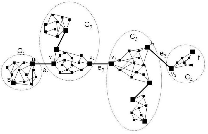
Figure 1: Decomposition D1.

With the above decomposition scheme at hand, we present an algorithm, termed Survivable Connection Addition (SCA), that returns an optimal solution to Problem 2CP-1 within polynomial time.

Algorithm SCA:

First step. We consider an instance $(G,s_{1},t_{1},s_{2},t_{2})$ with the same notations as above, such that the links of $G$ have a weight denoting their failure probability. In the graph $G_{2}$ representing the original graph $G$ without the links of $p_{1}$ and $b_{1}$, enumerate the bridge links, $e_{1},..,e_{r}$, that separate $s_{2}$ from $t_{2}$; these are the common links between the primary and the backup paths obtained by the tunable survivability algorithm of [1]. If $s_{2}$ and $t_{2}$ are not in the same connected component of $G_{2}$, go directly to the fourth step.

Second step. Decompose the joint connected component of $s_{2}$ and $t_{2}$ in $G_{2}$ into components $C_{1},..,C_{r+1}$ separated by the bridge links $e_{1},..,e_{r}$. - (i.e. Decomposition D1). For $1\leq l\leq r$, each bridge link $e_{l}$ has a pair of endpoints $(v_{l},u_{l+1})$ such that $v_{l}$ is in $C_{l}$ and $u_{l+1}$ in $C_{l+1}$. Define $u_{1}$ as $s_{2}$ and $v_{l+1}$ as $t_{2}$. Denote by $C_{i}$ (respectively, $C_{j}$) the closest component with a common node with $b_{1}$ from $C_{1}$ (respectively, $C_{r+1}$), if there are such components, and denote by $x_{i}$ (respect., $x_{j}$) a node of $b_{1}$ in $C_{i}$ (respect., $C_{j}$); see an example in Figure 1.

Third step. Consider the primary and backup paths obtained by [1] in $G_{2}$ with $s_{2}$ and $t_{2}$ as source and destination nodes. If $x_{i}$ and $x_{j}$ are in the same component, the algorithm returns this solution. Otherwise, the solution is returned at the end of this step. Add a fictitious link between these two nodes and compute two link-disjoint paths $p_{a}$ and $p_{b}$ from $u_{i}$ to $v_{j}$ in the new graph. Without loss of generality, we may assume that $p_{a}$ does not use the fictitious link. In particular, $p_{a}$ replaces the partial path of the primary path obtained by [1] between $u_{i}$ and $v_{j}$. The partial path of the backup path obtained by [1] between $u_{i}$ and $v_{j}$ is also replaced with three different partial paths. Between $u_{i}$ and $x_{i}$ the partial path is replaced by the partial path of $p_{b}$ between these two nodes. Between $x_{i}$ and $x_{j}$, the links of the first backup path $b_{1}$ are used; between $x_{j}$ and $v_{j}$ the partial path of $p_{b}$ between these two nodes is used.

Fourth step. The graph $G_{1}$ represents the original graph $G$ without the links of $p_{1}$. If $s_{2}$ and $t_{2}$ are not in the same connected component of $G_{1}$, no feasible solution can be found. We denote by $q_{1}$ the value of the failure probability of the second connection obtained by [1] for a connection request from $s_{2}$ to $t_{2}$ in $G_{1}$.

Fifth step. The primary path $p_{2}$ is obtained as the shortest path from $s_{2}$ to $t_{2}$ in $G_{1}$, where each link has the same weight as in $G$. The graph $G^{\prime}_{1}=(V^{\prime}_{1},E^{\prime}_{1})$ represents the original graph $G$ without the links of $b_{1}$, such that every link in $E^{\prime}_{1}$ has a zero weight except the links of $p_{1}$, which keep their original weights. The backup path $b_{1}$ is the shortest path from $s_{2}$ to $t_{2}$ in $G^{\prime}_{1}$. We denote by $q_{2}$ the failure probability of the second connection composed of these two paths.

Sixth step. If $q_{2}<q_{1}$, return the paths $p_{2}$ and $b_{2}$. Otherwise, return the paths obtained by [1] for a connection request from $s_{2}$ to $t_{2}$ in $G_{1}$.

Theorem 1

Algorithm SCA solves Problem 2CP-1 in $O(n~{}\cdot~{}m)$ steps.

Proof: We consider the three generic cases (shared backup, unavoidable first backup, overlapped connections) that corresponds to the optimization expression (5), as described above, and we analyze the optimality of the solution obtained by Algorithm SCA under each case, as well as the corresponding computational complexity.

Consider first the shared backup case: $p_{1}$ has no superposition with other paths, while $b_{1}$ potentially has some superposition with only $b_{2}$. We prove here that if we can find two paths for the second connection respecting the overlapping constraints of the shared backup case, this solution globally minimizes the failure probability of the second connection amongst all possible solutions.

Since there is no superposition with $p_{1}$, we can delete its links from the graph to get a new graph $G_{1}$. In a one-link connected graph, we can compute the minimal failure probability of a connection as the sum of the bridge links between the source and the destination as indicated by expression (3). We obtained a graph called $G_{2}$ by deleting the links of $b_{1}$. If $s_{2}$ and $t_{2}$ are not in the same connected component in $G_{2}$, no solution to the shared backup case can be found, since the second primary path $p_{2}$ should be link disjoint with both of the paths of the first connection. Thus the optimal solution can be found only within the two other cases (first step of SCA).

Otherwise, if $s_{2}$ and $t_{2}$ share the same connected component in $G_{2}$, we proceed with decomposition D1, listing the bridge links $\{e_{1},..,e_{r}\}$ of $G_{2}$ that separate $s_{2}$ from $t_{2}$ in successive connected components $\{C_{1},..,C_{r+1}\}$, as depicted in Figure 1. $s_{2}$ is located in $C_{1}$, and $t_{2}$ in $C_{r+1}$. We denote by $C_{i}$ and $C_{j}$ the components of lowest and highest index that have a common node ($x_{i}$ and $x_{j}$) with $b_{1}$ (Second step of SCA).

We claim that we can find two link-disjoint paths from $s_{2}$ to $t_{2}$ that form a connection respecting the shared backup case constraints and such that its failure probability equals the sum of the failure probabilities of the bridge links that are not between $C_{i}$ and $C_{j}$ (i.e. $\sum_{l=1}^{i-1}P_{f}(e_{l})+\sum_{l=j+1}^{r}P_{f}(e_{l})$). Indeed, if we add a fictitious link between $x_{i}$ and $x_{j}$, which stands for the partial path of $b_{1}$ that is forbidden to $p_{2}$ in this configuration, then in the new graph the bridge links that separate $s_{2}$ from $t_{2}$ are the same except the ones between $C_{i}$ and $C_{j}$. Thus, in this new graph, we select two paths that minimize the connection failure probability. Only one of them uses the additional link, and it should be $b_{2}$ (third step of SCA). In addition, this failure probability is minimal amongst the different cases: in the unavoidable first backup case, the same links have to be shared by the paths of the second connection since they are also bridge links in $G_{1}$. In the overlapped connection case, the failure probability of the second connection includes the one of the primary path $p_{2}$ and by its construction, $p_{2}$ uses all the bridge links between $s_{2}$ and $t_{2}$ in $G_{1}$. As a consequence, its failure probability is superior to that obtained by the shared backup case.

We consider now the unavoidable first backup case (fourth step). This case can be an improvement compared to the shared backup case only if $s_{2}$ is disconnected from $t_{2}$ in $G_{2}$. We handle this case by taking the best disjoint paths in $G_{1}$ without taking into account which links belong (or not) to $b_{1}$. We get for the failure probability of the second connection a value $q_{1}$ equal to the sum of the failure probability $p_{1}$ and failure probabilities of bridge links between $s_{2}$ and $t_{2}$ in $G_{1}$.

In the overlapped connection case, we can decouple the determination of the two paths of the second connection. We recall that in this case the only possible superpositions are between $p_{1}$ and $b_{2}$, $b_{1}$ and $p_{2}$, and $p_{2}$ and $b_{2}$. The establishment of the primary $p_{2}$ does not interfere with the choice of $b_{2}$, hence their establishment can be done independently. Indeed, according to the minimization expression (5), in this case the failure probability of the second connection can be expressed by $P_{f}(p_{2})+P_{f}(p_{1}\cap b_{2})$. Thus, we can take for $p_{2}$ the shortest path from $s_{2}$ to $t_{2}$ in $G_{1}$ (the weights are the failure probabilities of the links). The choice of $b_{2}$ corresponds then to a shortest path from $s_{2}$ to $t_{2}$ in a graph $G^{\prime}_{1}$ where the links of $b_{1}$ have been deleted from $G$ and the only positive weight links are the links of $p_{1}$ with their real failure probabilities (fifth step). Finally, we compare the solution between the two last different cases and we return its corresponding primary and backup paths (sixth step).

We proceed to prove the polynomial complexity of Algorithm SCA by determining the complexity time of each successive step. The first step can be computed in $O(n\cdot m)$ steps: if it exists, a bridge link should be on the shortest path between $s_{2}$ and $t_{2}$ that can be computed in $O(m+n\log n)$ time using Dijkstra’s algorithm [4]. For each link of the shortest path (less than $n$), we determine if it corresponds to a bridge link by removing it and by observing if there is some connectivity in the resulting graph between $s_{2}$ and $t_{2}$ ($O(m)$ steps). The second step can be done in $O(m)$ steps: after the removal of all the bridge links found in the first step, it checks only the connectivity of the different components.

The third step can be done in $O(m\log_{1+\frac{m}{n}}n)$ steps: we can improve the complexity time of [1] by duplicating all the bridge links found in the first step and computing in the resulting graph the two link-disjoint paths according to Suurballe-Tarjan’s algorithm [22], which runs in $O(m\log_{1+\frac{m}{n}}n)$ number of steps. The fourth step has the same complexity since the verification of a shared connected component in $G_{1}$ between $s_{2}$ and $t_{2}$ can be done with Dijkstra’s algorithm, and the computation of the improved algorithm inspired from [1] has been established in the third step. At last, only successive shortest path computations are done in the fifth step, in $O(mn\log n)$ time.  

In Problem 2CP-2, the primary path $p_{1}$ has been established already, and a backup path $b_{1}$ and the two paths of the second connection should be found such the failure probability of the second connection is minimized while providing zero failure probability to the first connection (i.e., obeying the constraint $MCFP(c_{1})=0$). As a consequence, the two paths of the first connection must be link-disjoint. We proceed to prove the computational intractability of Problem 2CP-2.

Theorem 2

Problem 2CP-2 is NP-complete; moreover, it is NP-hard to approximate its solution within a constant factor.

Proof:

We shall employ a reduction to the shortest path with pairs of forbidden nodes problem (termed Problem SP-DPFN). As shown in [3], the special case of Problem SP-DPFN where the degree of the forbidden nodes is equal to two (termed Problem SP-DPFN2) is Min-PB[11]; the latter is a class of minimization problems whose objective functions are bounded by a polynomial in the size of the input. Problems of this class are hard to approximate, which implies that Problem SP-DPFN2 is NP-complete and it is NP-hard to approximate its solution within a constant factor.

We consider an instance $(G,w,s,t,W)$ where $G=(V,E)$ is the graph of the instance, $w$ its weight function, $s$ and $t$ are, respectively, the source and the destination, and $W$ is the collection of the disjoint pairs of forbidden nodes. We apply the following clique transformation to $G$. Each node with a degree larger than two is transformed into a clique whose number of nodes equals the degree of the original node and the internal links have zero weight (see Figure 2). We obtain a new graph called $G_{1}=(V_{1},E_{1})$. For each clique in $G_{1}$representing a node $x_{i}$ in $V$ and each link $(x_{i},x_{j})$ in $E$, we call $x_{i}^{(x_{j})}$ the node of this clique which is linked to a node of the clique in $G_{1}$ representing $x_{j}$ ($x_{j}\in V$).

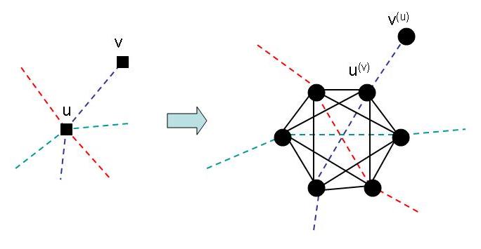
Figure 2: The clique transformation.

This transformation can be done within a polynomial number of steps. Even in the worst case of a clique $K_{n}$ (with $n$ nodes and $m=\frac{n(n-1)}{2}$ links) as the original graph, after the clique transformation, the obtained graph will be composed of $n(n-1)$ nodes and $\frac{n(n-1)^{2}}{2}$ links, since each node has a degree $n-1$.

The subproblem of SP-DPFN2 where the graph of the instance has been transformed by a clique transformation remains intractable. Indeed, an immediate correspondence can be found between paths of both instances. In addition, even if we assume that $G$ is Eulerian, this restriction does not modify the tractability of the SP-DPFN2 problem for an instance with $G$ as the graph.

We consider an instance $(G,w,s,t,W)$ of the SP-DPFN2 problem, such that the original undirected graph $G$ is Eulerian and has been transformed to $G_{1}=(E_{1},V_{1})$ by the clique transformation. $s$ and $t$ are, respectively, the source and the destination of the shortest path. The collection of disjoint forbidden pairs of nodes $W$ includes $\{(x_{1},y_{1}),..,(x_{l},y_{l})\}$. We build from this instance a new instance to Problem 2CP-2 as follows. We add two nodes $s^{\prime}$ and $t^{\prime}$ to $V_{1}$ and we link them to the source $s$ and to the destination $t$ of the shortest path (i.e. we add $(s^{\prime},s)$ and $(t^{\prime},t)$ to $E_{1}$). We transform each node of the different pairs of forbidden nodes according to the following “bow tie” transformation.

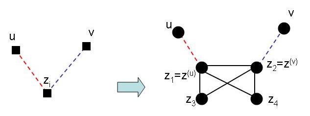
Figure 3: The bow tie transformation.

As described in Figure 3, with this transformation a node $z_{i}$ with a degree two is split into four interlinked nodes $\{z_{i}^{1},z_{i}^{2},z_{i}^{3},z_{i}^{4}\}$, with additional links of zero weight $\{(z_{i}^{1},z_{i}^{3}),(z_{i}^{2},z_{i}^{4}),(z_{i}^{1},z_{i}^{4}),(z_{i}^{2},z_{i}^{3})\}$. In addition, both $z_{i}^{1}=z_{i}^{(u)}$ and $z_{i}^{2}=z_{i}^{(v)}$ are endpoints of the respective outgoing links $(z_{i},u)$ and $(z_{i},v)$. (We note that $z_{i}^{1}$ and $z_{i}^{2}$ are linked by a positively weighted link.) We will see that this link is necessarily used by the primary path $p_{1}$. Beyond this transformation, we add a new node set $V_{2}=\{v_{1},..,v_{l+1}\}$ and the link set $F_{2}=\{(s,v_{1}),(v_{i},x_{i}^{3}),(v_{i},y_{i}^{3}),(x_{i}^{4},v_{i+1}),(y_{i}^{4},v_{i+1}),(v_{l+1},t),1\leq i\leq l\}$ such that each link has a zero weight. Finally, we take $s_{1}=s_{2}=s$ and $t_{1}=t_{2}=t$.

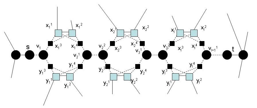
Figure 4: The reduction for Problem 2CP-2.

Figure 4 sums up this new instance composed of a graph $G^{\prime}=(V^{\prime},E^{\prime})$. For ease of drawing, the regular nodes of $G$ are not included. We assume that $p_{1}$ has been chosen in order to go through all the nodes in the original graph $G$ (which is possible because $G$ is Eulerian). Thus, if $p_{1}=(r_{1},..,r_{i},..,r_{j},..,r_{n})$ such that $r_{i}$ is assumed to be a member of a pair of forbidden nodes and $r_{j}$ a regular node, the primary path $p_{1}$ will be composed of $r_{i}^{(r_{i-1})}-r_{i}^{(r_{i+1})}$ instead of $r_{i}$, and of $r_{j}^{(r_{j-1})}$ and $r_{j}^{(r_{j+1})}$ instead of $r_{j}$.

Assume we have an algorithm that solves Problem 2CP-2. In addition, instead of a uniform weight distribution, assume that the weight of links of type $(z_{i}^{1},z_{i}^{2})$ are identical and equal to $m$ times the uniform weight of the other weighted links. Since $s$ and $t$ have a node degree of two, the shared backup case is not relevant here. The optimal solution is thus due to the unavoidable first backup case or to the overlapped connection case. In the first case, the three paths $b_{1},p_{2}$ and $b_{2}$ can only use the additional zero weight links, since these paths should be link-disjoint with $p_{1}$. Thus, by taking an identical path from $s$ to $t$ through these zero weight links, we get that the failure probability of the second connection is equal to $P_{f}(p_{1})$. Considering the overlapped connection case, for the same reasons $b_{1}$ and $p_{2}$ are allowed to use only zero weight links. Since in this case the failure probability of the second connection is $P_{f}(p_{1}\cap b_{2})$ (we recall that $P_{f}(p_{2})=0$), the minimal failure probability of the second connection reflects the number of links of kind $(z_{i}^{1},z_{i}^{2})$ used because of their relatively large weight. Moreover, the backup path $b_{2}$ only uses links present in the original graph $G$ except maybe some links of the bow ties. The backup path may go through $z_{i}^{1}$ and $z_{i}^{2}$ without using the link $(z_{i}^{1},z_{i}^{2})$ only if both the backup path $b_{1}$ and the primary path $p_{2}$ do not go neither through $z_{i}^{1}$ nor $z_{i}^{2}$. Thus, by evaluating the minimal failure probability of the second connection, we are able to deduce if a link of kind $(z_{i}^{1},z_{i}^{2})$ has been used. If no such link has been used, this backup path $b_{2}$ is the shortest path in $G$ from $s$ to $t$ that does not use both nodes of any pair of forbidden nodes. Thus this path would solve the SP-DPFN2 problem for this instance.

Conversely, from any solution to the SP-DPFN2 problem with the original instance we can construct a solution to Problem 2CP-2, as follows. We consider for the overlapped connection case the backup path $b_{2}$ that corresponds to the respective path in $G^{\prime}$, and for $b_{1}=p_{2}$ a path that is composed of zero weight links and is link disjoint with $b_{1}$ (such a path exists, since the initial shortest path does not use both nodes of a pair of forbidden nodes). As we have seen, this combination leads to the minimal failure probability for the second connection in the overlapped case, and the solution is obtained by comparing it to the failure probability of the solution obtained in the unavoidable first backup case (i.e. $P_{f}(p_{1})$).  

We are ready to present our heuristic scheme for solving Problem 2CP-2, termed Algorithm 2CP-2A. The basic idea of this algorithm is to return the best solutions in the shared backup case (first step of Algorithm 2CP-2A) and the unavoidable first backup case (second step of Algorithm 2CP-2A). We do not consider the solutions that respect the constraints of the overlapped connection case, because, as indicated in the proof of Theorem 2 (presented in [tr]), they are the source of the intractability of Problem 2CP-2. In addition, Algorithm 2CP-2A always returns a (not necessarily optimal) solution if there exists at least one solution $\{(b_{1},p_{2},b_{2})\}$ that respects the constraints of the overlapped connection case. For example, the solution with the same paths except that the second backup path is chosen identical to $p_{2}$, respects the constraints of the unavoidable first backup case since both paths of the second connection are link-disjoint with the first primary path.

Algorithm 2CP-2A:

First step. In the graph $G_{1}$ representing the original graph $G$ without the links of $p_{1}$, find two link-disjoint paths, one from $s_{1}$ to $t_{1}$, the other from $s_{2}$ to $t_{2}$, using the two link-disjoint path algorithm of [23]. If such paths are found, assign for $b_{1}$ the path from $s_{1}$ to $t_{1}$. Then, given the two paths of the first connection, assign to the second connection the paths returned by Algorithm SCA.

Second step. If no such paths are found, assign to $b_{1}$ the shortest path from $s_{1}$ to $t_{1}$, and assign to the second connection the paths obtained by [1] in $G_{1}$.

In Section V we shall present the results of a simulation study on the performance of Algorithm 2CP-2A.

We proceed to consider Problem 2CP-3. Here, four paths should be found such that the first connection is fully reliable (namely, $MCFP(C_{1})=0$), and the paths of the second connection minimize its failure probability. Similarly to Problem 2CP-2, we prove the hardness of Problem 2CP-3 and, based on the insight gained through this analysis, we propose heuristic solution schemes.

Theorem 3

Problem 2CP-3 is NP-complete; moreover, it is NP-hard to approximate its solution within a constant factor.

Proof: We shall employ a reduction from 2CP-3 to Problem SP-DPFN2 (in its nodal version), similarly to the previous proof. SP-DPFN2 remains Min-PB even in its nodal version[3], which implies that Problem SP-DPFN2 and thus Problem 2CP-3 is NP-complete and it is NP-hard to approximate it within a constant factor.

We consider the graph used in the proof of Theorem 10. In addition, we transform all the links in the original graph $G$ according to the following duplicate link transformation.

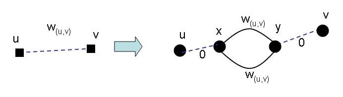
Figure 5: The duplicate link transformation.

As depicted in Figure 5, with the duplicate link transformation, we create, out of a link $(u,v)$, two additional internal nodes $x$ and $y$, and four replacing links $\{(u,x),(x,y),(x,y),(y,v)\}$ such that $w_{(u,x)}=w_{(y,v)}=0$ and $w_{(x,y)}$ is equal to the previous $w_{(u,v)}$ for both links $(x,y)$. Our goal is to determine the existence of a solution that leads to a zero failure probability for the second connection. Since the sources and the destinations are identical ($s_{1}=s_{2}=s$ and $t_{1}=t_{2}=t$) and their degree is equal to two, there is no need to consider the shared backup case similarly to the previous proof. Indeed, finding paths that respect the constraints of the shared backup case would imply that at least three link-disjoint paths emanate from $s$ (namely, the two primary paths and the shared backup path), which is impossible. In the unavoidable first backup case, the total second connection failure probability includes the path failure probability of the first primary path $p_{1}$ (since $p_{1}$ and $b_{1}$ have no common links), which should thus equal zero. Therefore, $p_{1}$ is allowed to use only the zero weighted links. Thus, finding a zero failure probability for the second connection is equivalent to finding a path in the original graph that includes at most one node of each pair of forbidden nodes. In addition, by minimizing the failure probability of the second connection, we aim to find in the reduced problem the shortest path, which is a Min-PB problem. In the overlapped connection case, the total failure probability of the second connection includes the path failure probability of the second primary path $p_{2}$. Similarly, this path is allowed to use only zero weighted links, i.e. the links with zero failure probability. Once again, if we take, for example, $b_{1}=p_{2}$ (it does not add any constraint), getting a zero failure probability for the second connection means finding in the original graph, for the first primary path $p_{1}$, a path including at most one node of each pair of forbidden nodes.

Conversely, any solution to the SP-DPFN2 problem in its nodal version leads to an optimal solution for Problem 2CP-3. Indeed, we can take as $b_{1},p_{2}$ and $b_{2}$ the same paths corresponding to the solution of problem SP-DPFN2, such that the only unshared links between $p_{2}$ and $b_{2}$ are the weighted links. In addition, we select the first primary path from $s$ to $t$ such that only zero weighted links are used. There exists at least one feasible path because the solution of the SP-DPFN2 problem does not use both nodes of each pair of forbidden nodes.  

We proceed to describe two heuristics for Problem 2CP-3, both of which are evaluated by way of simulations, as described in Section V. In both heuristics, we decouple Problem 2CP-3 into two problems. For the first heuristic, termed Algorithm 2CP-3A, we first assign the paths of the first connection, and, with these at hand, we proceed to choose the paths of the second connection by employing our (optimal) solution to Problem 2CP-1. In the second heuristic, termed Algorithm 2CP-3B, we first choose the primary path of the first connection, $p_{1}$, and, with this at hand, we choose the other paths by employing our (heuristic) solution to Problem 2CP-2. The first selection in both heuristics is done in a way that attempts to minimize interference with the next connection; this is done by employing a heuristic rule similar to that of the MIRA scheme [14], i.e., the link weights attempt to reflect their “criticality”. The choice of the weight function is crucial for the success of such schemes, and several functions are proposed in [14] that are correlated to the link residual bandwidth. In order to avoid links that form part of small link cuts (e.g. bridge links) in the choice of the paths, we define a weight function as follows.

Definition 6

Given an undirected graph $G=(V,E)$ and a “level” $l$, the small-cut weight of a link $e$ is:

$$w_{e}=\sum_{i=1}^{l}\frac{n_{i}}{i}\$$ (8)

where $n_{i}$ denotes the number of small cuts of size (exactly) $i$ including $e$, for $1\leq i\leq l$.

In order to compute these small-cut weights, we use the polynomial time algorithm of [19], which computes, for an unweighted graph, the list of the small cuts up to a specified level $l$.

Algorithm 2CP-3A:

First step. Considering link weights according to the small-cut weight function (Expression 8), execute Suurballe-Tarjan’s algorithm[22]. Assign the two link-disjoint paths that it outputs to the first connection.

Second step. Given the outcome of the first step, employ Algorithm SCA in order to select the paths of the second connection.

Algorithm 2CP-3B:

First step. Select for $p_{1}$ the shortest path from $s_{1}$ to $t_{1}$ using any standard shortest-path algorithm (e.g. Dijkstra [4]), such that the link weight are obtained by the small cut weight function.

Second step. Given the outcome of the first step, employ Algorithm 2CP-2A in order to select the remaining three paths.

III-D Unreliable First Connection

Theorem 4

For a general value of $MCFP(c_{1})$, Problem 2CP-1 is NP-hard.

Proof: The proof can be found in the Appendix (Theorem 9).  

III-E Reliable Second Connection in an Offline Framework

Theorem 5

The problem of determining if the optimal solution of Problem 2CP-3 results in two connections fully reliable is computationally tractable.

Proof: The problem is equivalent to Problem 2-CESB, which is proven in the Appendix to be computationally tractable (Theorem 11).  

IV Extension to $K$ Connections

We proceed to consider Problem KCP, namely the problem of establishing some $K$ connections, $K>2$. We have seen that, for Problem 2CP, the computational tractability (or lack thereof) of the problem variants depend on the level of reliability demanded by the connections (namely, whether they require full reliability or not), as well as on whether an online or offline framework is considered.

More specifically, we have seen that, in both online and offline frameworks, Problem 2CP is intractable when not all the connections are required to be fully reliable. One exception is Problem 2CP-1, which considers an online framework in which the second connection is not required to be fully reliable. However, this exception is quite artificial under an online framework when the number of connections is unknown in advance: if we tolerate the last connection to be unreliable, the establishment of an (unknown) future request will become intractable.

In view of the above findings, when moving to consider more than two connections we restrict our attention to fully reliable connections. We begin with a brief overview of known results on the related $K$ disjoint paths problem. We then formulate an online variant of Problem KCP, for which we establish a polynomial-time optimal solution. We then discuss the tractability of several extensions of the online problem. Finally, we show that the offline version is also computationally tractable.

IV-A The $K$ Disjoint Path Problem

The $K$ disjoint path problem is, in fact, the problem of establishing multiple connections, each consisting of only a single path (i.e., no backup paths). Formally, the problem is as follows. Given a collection of pairs of nodes $\{(s_{1},t_{1}),..,(s_{K},t_{K})\}$ in a graph $G=(V,E)$, find $K$ mutually disjoint paths from $s_{i}$ to $t_{i}$ for each $1\leq i\leq K$. For a general value of $K$, this problem is known to be amongst the “classic” NP-Hard problems [12], both in its link-disjoint and node-disjoint versions. On the other hand, if $K$ is fixed, i.e., $O(1)$, the problem is, in principle, solvable in polynomial time, but the existing solutions involve the computation of constant factors that are, in practice, computationally prohibitive for $K>2$ (yet they are practically admissible for the case $K=2$) [23]. For a fixed ($O(1)$) value of $K$, polynomial solutions have been established, both for planar graphs [20] and for general graphs [21].

The tractability of the weighted version of the problem, i.e. minimizing the total weight of all the $K$ disjoint paths (for a fixed $K$ and given a weighted graph), is an open problem even for $K=2$.

IV-B The Online $K$ Connection Problem

IV-B1 Problem Formulation

We focus on an online version of the $K$ connection problem, for $K>2$. In this setting, at each step $K$, we check whether we can establish a new connection between a source $s_{K}$ and a destination $t_{K}$, given the paths allocated to the previous connections at steps $1,2,\cdots,K-1$. At this stage, we can distinguish between three disjoint sets of links, which partition the original graph. The first set is the set of free links (that is, links not already used by any paths), the set of backup links (links only shared by previous backup paths), and the set of the primary links (links only used by some primary path). For the new connection, we allow its primary path to use only free links, while its backup path is allowed to use free as well as backup links.

Definition 7

For an instance $I=(G,E_{1},E_{2},E_{3},s_{k},t_{k})$, where $G=(V,E)$ is an unweighted undirected graph, $E_{1},E_{2}$ and $E_{3}$ form a partition of the link set $E$, corresponding to the link sets of free, backup and primary links (respectively), and $(s_{K},t_{K})$ are two nodes of $V$, the online $K$ connection problem (in short, OKCP) is the problem of finding two link-disjoint paths from $s_{K}$ to $t_{K}$ (“primary” and “backup”) such that none of the two paths uses any primary links (i.e., links of $E_{3}$) and at most one of the paths uses backup links (i.e., links of $E_{2}$).

IV-B2 Reduction for Problem OKCP

Lemma 1

For each instance of Problem OKCP, there is a reduction R1 to an instance where $s_{K}$ and $t_{K}$ are in the same two-link connected component of the graph formed by the union of $E_{1}$ and $E_{2}$.

Proof: Given an instance $I_{1}=(G,E_{1},E_{2},E_{3},s_{K},t_{K})$, if $s_{K}$ and $t_{K}$ are not in the same two-link connected component of the graph formed by the union of $E_{1}$ and $E_{2}$, by Menger’s Theorem[18] we are ensured that no two link-disjoint paths from $s_{K}$ to $t_{K}$ can be found, even if we allow both paths to use free and backup links.  

The previous lemma gives a necessary condition for the existence of a solution to Problem OKCP. Unfortunately, and in contrast to the setting covered by Menger’s Theorem, in our case the primary path between $s_{K}$ and $t_{K}$ cannot use the backup links, hence the condition is not sufficient, as demonstrated in Figure 6. This figure depicts the free links and the two first backup paths $b_{1}$ and $b_{2}$ (the respective primary paths are not drawn). Despite that $E_{1}\cap E_{2}$ forms a two-link connected graph, a new request between $s$ and $t$ must be declined. We thus proceed with a more detailed study of the characterization of the solution’s feasibility.

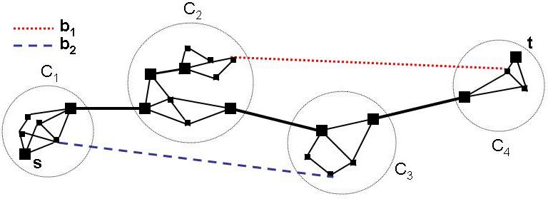
Figure 6: Menger’s Theorem is not enough.

IV-B3 Leaps and Transitions

According to the previous reductions, we can consider from now on that $E_{1}\cup E_{2}$ forms a two-link connected graph such that $E_{1}$ is one-link connected and all its bridge links separate $s_{K}$ from $t_{K}$ . The result is very similar to the one obtained after the decomposition D1, except that here all the components are necessarily two-link connected. In order to determine the existence of a solution to Problem OKCP, we decompose the problem according to the two-link connected components of $E_{1}$. For each component, we analyze which are the link-disjoint paths that may be part of a solution (if such a solution exists), and then we determine if the instance is solvable. We shall need the following definitions.

Definition 8

Given a pair of nodes $\{u,v\}$, a source $s$ and a destination $t$, we say that a path $p$ from $s$ to $t$ has a leap $\{u,v\}$ if $p$ is composed of two link-disjoint paths corresponding either to a path from $s$ to $u$ and another path from $v$ to $t$, or to a path from $s$ to $v$ and another path from $u$ to $t$.

Definition 9

Given a two-link connected component of free links, including four nodes $\{s_{1},t_{1},s_{2},t_{2}\}$ and a set $B$ of nodes of this component connected to a backup link, a leap set $\{(u_{1},v_{1}),..,(u_{k},v_{k})\}$ is called a feasible transition if all the nodes of the leap set are in $B$, and we have two link disjoint paths, one from $s_{1}$ to $t_{1}$, and the other from $s_{2}$ to $t_{2}$ with the leaps of the leap set.

Given a two-link connected component $C$ of free links with four nodes $\{s_{1},t_{1},s_{2},t_{2}\}$, we specify in the Appendix the conditions on the instance $(C,s_{1},t_{1},s_{2},t_{2})$ for admitting a transition without any leap. In addition, we can use a $K$ link-disjoint path algorithm[21] to determine the existence of a transition with $K-1$ leaps. Thus we can list all the possible transitions for each component, for any number of leaps. We proceed with a specification of the algorithm that solves Problem OKCP.

IV-B4 Algorithm RCA

We present here the Reliable Connection Addition algorithm (Algorithm RCA), that returns a solution to Problem OKCP if there is one, and indicates its absence otherwise.

First step. Let $G_{1}$ be the graph of free links. Denote by $C_{1}$ the connected component in $G_{1}$ to which $s_{1}$ belongs. If $t_{1}$ is not located in this component, return no solution. Otherwise, assign all the free links not in $C_{1}$ to the backup link set $E_{2}$.

Second step. If $G_{1}$ is a two-link connected graph, we can find two link-disjoint paths from $s_{K}$ to $t_{K}$ using only links of $E_{1}$. Else if $E_{1}\cap E_{2}$ contains a bridge link that separates $s_{K}$ from $t_{K}$, return no solution (Reduction R1).

Third step. Consider all the possible combinations of backup link sets with no redundancy by progressively incrementing the maximal number $N_{1}$ of leaps by transition, as follows.

$N_{1}\leftarrow 0$

  while $N_{1}<K$ do

     compute all the possible transitions with at most $N_{1}$ leaps; observe if there is at least one combination that goes from the first component to the last one, such that all the transitions are feasible and in different components, and such that for each leap $(u,v)$ there is a corresponding path in another component from the backup link set of $u$ to the one of $v$. If a feasible combination is found, go to the fourth step, else increment $N_{1}\leftarrow N_{1}+1$

  end while

Stop when $N_{1}=K$ and return no solution.

Fourth step. Compute the respective transitions and return the feasible primary and backup paths.

Theorem 6

Algorithm RCA solves Problem OKCP within $O(max(n^{4},n^{K-2}))$ steps.

Proof: The first step verifies that $s_{K}$ and $t_{K}$ are in the same connected component $C_{1}$ for an eventual path $p_{K}$. Otherwise, no feasible solution can be found. The assignment of the free links not in $C_{1}$ to $E_{2}$ does not modify the number of solutions since no primary path $p_{K}$ will be able to use these free links. We use Lemma 1 to ensure that no bridge links separate $s_{K}$ from $t_{K}$ in the graph formed by $E_{1}\cap E_{2}$. We recall that after this assignment, the number of connected components of $E_{2}$ is inferior or equal to the number of backup paths, i.e. $K-1$, because each backup set has at least a backup link that a backup path uses with an endpoint in $G$.

In the third step, proceeding by induction on the maximal number of leaps by transition, we consider all the possible combinations of backup link sets that could lead to a solution. Indeed, if a solution exists, its maximal number of leaps for a transition cannot be more than $K-1$, since a backup link set cannot be used twice for a given transition. Thus, by Algorithm RCA, a solution is found only if one exists, and the solution returned is such that the maximal number of leaps by transition is minimal. In the fourth step, the computation of the primary and backup paths that use these transitions is done in order to return paths that would form a feasible $K$th connection.

The number of considered combinations remains polynomial since the length of each cannot be greater than the bounded number of link backup sets. Thus, the algorithm runs in polynomial time. We proceed to compute the running time of Algorithm RCA. The first step needs $O(m)$ to verify that $s_{1}$ and $t_{1}$ are in the same shared connected component. The second step runs in $O(n\cdot m)$ number of steps, since it looks for the bridge links between $s_{K}$ and $t_{K}$ both in graphs $G_{1}$ and $E_{1}\cap E_{2}$. As seen in the proof of Theorem 1, bridge links between separating two nodes can be found in $O(n\cdot m)$ steps. In addition, if no bridge edge is found between $s_{K}$ and $t_{K}$ in $G_{1}$, we use Suurballe-Tarjan’s algorithm that runs in $O(m\log_{1+\frac{m}{n}}n)$ time when returning the solution.

In the third step, the number of combinations is constant regarding to $n$ since it depends only on the number of backup link sets, which is bounded by $K-1$. For each component $C_{i}$, we can compute all its possible transitions by ignoring the other components and in $O(n^{4})$ steps: we remove all the edges (including the bridge edges separating $s_{K}$ from $t_{K}$) in $G_{1}$ which are not part of the component and all the backup link sets that have no common node with $C_{i}$. We denote by $a_{i}$ and $b_{i}$ the two nodes of $C_{i}$ that should be linked only by free links in order to be part of the primary path. In addition, in $E_{2}$, we replace each set $S$ of the remaining backup link sets by a single node $x_{S}$ linked to all the common nodes of this set with $C_{i}$. At last, we transform all the nodes endpoints of free links according to the clique transformation (see the proof of Theorem 2 for its definition). This transformation can be done in $O(m)$ steps: we first compute the degree of each node in order to create a corresponding number of nodes in the transformed graph, and then we assign the linkage according to each link in the original graph. Thanks to the clique transformation, the computation of link-disjoint paths in the original graph is equivalent to the computation of node-disjoint paths in the transformed graph by an immediate correspondence. Moreover, since we have not transformed the added nodes $\{x_{S}\}$, the computation of node-disjoint paths in the resulting graph prevents us from receiving a primary path using backup links. Indeed, for a specified component and for a combination of backup link sets $\{(S_{1},..,S_{2r}),r\leq N_{1}\}$, we use the disjoint path algorithm [21] (which runs in $O(n^{3})$ time) in its nodal version to find the $r+1$ node-disjoint paths that would compose the transition. These paths are $\{(a_{i},b_{i}),(x_{2l-1}l,x_{2l})|1\leq l\leq r\}$. Since we do the computation of all the transitions for $O(n)$ components, the resulting number steps is $O(n^{4})$.

Once we have listed all the transitions with less than $N_{1}$ leaps for each component, we observe if a given combination $\{(S_{1},..,S_{j})\}$ can result to feasible primary and backup paths. We denote $c$ the number of components ($c\leq n$). This verification is time-consuming and can be done in $O(n^{K-2})$ steps: we consider all the possibilities where $(S_{i},S_{i+1}),1\leq i\leq j-1$ is in the $h^{(}i)$-th component, $1\leq h^{(}i)\leq c$. For this possibility, we verify if in each of the $j-1$ chosen components there is a feasible transition composed exactly of these backup link sets. Since we know that $S_{1}$ and $S_{j}$ should have a common node with the first and last component respectively, the possibility is characterized by the chosen components $\{h^{(}i),1\leq i\leq j-1\}$ and the number of possibilities is $O(n^{(}K-2))$ because $j$ is inferior or equal to $K-1$ (the maximal number of backup link sets).

When such a possibility is found, the fourth step computes the primary and backup paths according to this result.  

IV-B5 Heuristic Improvements

Beyond Algorithm RCA, heuristic improvements can be done in order to find faster a solution. These improvements can be a reduction of the graph of free links, or an interference minimization consideration, or a tradeoff between quality of the solution and computation time.

Lemma 2

For each instance of Problem OKCP, there is a reduction R2 to an instance where $E_{1}$ is exactly a one-link connected subgraph including $s_{K}$ and $t_{K}$ in separated two-link connected components, such that all the bridge links in $E_{1}$ separate $s_{K}$ from $t_{K}$.

Proof: We consider an instance $I_{1}=(G,E_{1},E_{2},E_{3},s_{K},t_{K})$. $s_{K}$ and $t_{K}$ should be in a common connected component of $E_{1}$ otherwise no feasible primary path could link $s_{K}$ to $t_{K}$ with only free links. Moreover, the primary path is not able to access the other connected components of $E_{1}$, while the backup path may be able to do so. Consequently, we can assign the links of the other components of $E_{1}$ to the backup link set $E_{2}$. We can then reduce $E_{2}$ to only its connected subgraphs having a node in common with $E_{1}$ (the other backup links are not accessible to the backup path). We observe that the number of connected subgraphs of $E_{2}$ is bounded by the number of connections already established (i.e. $K-1$): each backup path cannot be in more than a single connected component, since it forms a connected path. In addition, each connected subgraph of $E_{2}$ includes at least a backup path, otherwise it would have no common node with $E_{1}$. Moreover, $s_{K}$ and $t_{K}$ are in separated two-link connected components of $E_{1}$: otherwise, by Menger’s Theorem[18], we could (easily) find two link-disjoint paths from $s_{K}$ to $t_{K}$ using only free links, which would solve Problem OKCP for this instance.

We can reduce $E_{1}$ such that the only bridge links are the links separating $s_{K}$ from $t_{K}$. Indeed we consider another bridge link $e$ that separates $E_{1}$ into three edge sets $e\cup F\cup F^{\prime}$, such that $F$ and $F^{\prime}$ are connected and $s_{K}$ and $t_{K}$ are in $F$. Without modifying the feasibility of the solution, we can assign $e$ and the links in $F^{\prime}$ either to the backup link set if $F^{\prime}$ and $E_{2}$ have at least a common endpoint, or to $E_{3}$ otherwise. Indeed no primary path can use these links without using $e$ twice, and this is also the case for the backup path if $F^{\prime}$ and $E_{2}$ have no common endpoint. In addition, since we have not created new connected components, the number of backup link connected components is still bounded by $K-1$.  

As in the case of two connections, we can heuristically improve the success probability of future connections by minimizing the “interference” with the (unknown) future connections. Thus, we should assign weights to the links such that they reflect their “criticality”. Accordingly, we modify the last step of the algorithm as follows: we compute the primary path as before, and, given the primary path, we minimize the weight of the backup path from $s_{K}$ to $t_{K}$ in the graph formed by the union of $E_{1}$ with $E_{2}$. The weight of a link in $E_{1}$ corresponds to its criticality as defined by the small cut weight function in the graph of free links. The weights of links in $E_{2}$ is zero since they do not interfere with future primary paths.

In addition, there is an inherent tradeoff between quality of the solution and computation time. Indeed, the computation time of this algorithm is not polynomial in the bounded number of backup link sets. Moreover, we cannot hope to find such an algorithm: the respective Problem OKCP for a general $K$ can be easily reduced to Problem 2DPFL, which is proven in the Appendix to be NP-hard. Thus, it may be interesting to keep a rather small number of backup link sets for each new connection establishment. For future connections, the number of backup link sets does not increase only if the actual backup path goes through at least one endpoint of previous backup links. Consequently, if in the interference minimization of the backup path, the chosen backup path increases the number of backup link sets, we should compare its total weight to the minimal weight of a backup path going through at least an endpoint of a backup link (this comparison can be done in polynomial time).

IV-C Intractable Extensions

We proceed to indicate the intractability of several extensions of Problem KCP.

IV-C1 Directed Networks

For directed networks, multi-connection establishment problems are generally NP-Hard. Indeed, even the establishment of two connections without backup paths is already intractable: the two disjoint path problem was shown to be intractable, both in its nodal as well as its link versions[6].

IV-C2 Unbounded $K$

Theorem 7

For a general (not $O(1)$) $K$, Problem KCP is NP-complete. Moreover, it is NP-hard to approximate it within a constant factor.

Proof: The proof can be found in the Appendix (Theorem 15).  

IV-D The Offline $K$ Connection Problem

We proceed to consider the offline version of the $K$ connection problem. Here, the set of connections is given and the objective is to establish all of them at once. We proceed with a formal definition of the problem.

Definition 10

For an instance $I=(G,s_{1},t_{1},..,s_{k},t_{k})$, with $G=(V,E)$ an unweighted undirected graph, and $\{(s_{i},t_{i}),1\leq i\leq K\}$ source-destination pairs of $K$ connections, the offline $K$ connection problem (in short, OffKCP) is the problem of finding $2K$ (“primary” and “backup”) paths from $s_{i}$ to $t_{i}$, for $1\leq i\leq K$, such that no link can be shared by a primary path and another (primary or backup) path.

Theorem 8

For a fixed $K$, there is an optimal solution to Problem OffKCP of polynomial time complexity.

Proof: The proof can be found in the Appendix (Theorem 13).  

V Simulation Study

We performed simulations in order to evaluate the efficiency of our proposed heuristics, namely Algorithm 2CP-2A for Problem 2CP-2 and Algorithms 2CP-3A and 2CP-3B for Problem 2CP-3. These algorithms are compared with the optimal values (obtained through a “brute force” solution with an inherently prohibitive computational complexity), as well as with the outcome of more straightforward heuristic alternatives.

First, we describe the various algorithms that have been compared for each of the problems, namely Problems 2CP-2 and Problem 2CP-3. We then detail the network topology and the parameters chosen for the simulations. Through these simulations, we show the efficiency of our heuristics and discuss its causes.

V-A The Tested Algorithms

V-A1 Problem 2CP-2

We recall that, in this problem, the primary path of the first connection, $p_{1}$, is given. In our experiments, it was chosen to be the shortest path between $s_{1}$ and $t_{1}$. We then compared three algorithms for selecting the first backup path $b_{1}$ and the two paths, $p_{2}$ and $b_{2}$, of the second connection. We recall that these paths need to be selected so as to minimize the failure probability of the second connection. The three algorithms were the following: a simple heuristic (termed Algorithm 2CP-2N), our heuristic (Algorithm 2CP-2A), and an optimal (brute force) algorithm (2CP-2BF).

Algorithm 2CP-2A has been described in Section III. We detail here the other two algorithms. In the simple heuristic 2CP-2N, the links of $p_{1}$ are removed and we choose for $p_{2}$ the shortest path between $s_{2}$ and $t_{2}$ , where the link weights are their failure probabilities. If, after the removal of $p_{2}$, a path between $s_{1}$ and $t_{1}$ can be found, we choose it for the backup path $b_{1}$ and we then select for the backup path $b_{2}$ a path that minimizes the failure probability of the second connection given $p_{1}$, $p_{2}$ and $b_{1}$; otherwise, we do not remove the links of $p_{2}$ and we select for the backup path $b_{1}$ the shortest path from $s_{1}$ to $t_{1}$. We then select $b_{2}$ such that the failure probability of the second connection is minimized.

The optimal, brute-force algorithm 2CP-2BF computes all the possible backup paths $b_{1}$ from $s_{1}$ to $t_{1}$ link-disjoint from $p_{1}$, and it then applies Algorithm SCA for each pair of paths. This way, Algorithm 2CP-2BF always returns paths that minimize the failure probability of the second connection.

V-A2 Problem 2CP-3

In Problem 2CP-3, no path is already established but $p_{1}$ is constrained to be link-disjoint at least with $b_{1}$ and $p_{2}$. Our goal is to minimize the failure probability of the second connection. We compared five algorithms.

Similarly to Algorithm 2CP-3A, the first algorithm (termed 2CP-3N) select at first the two paths of the first connection with Suurballe-Tarjan’s algorithm[22], and then the second connection with Algorithm SCA. The only difference between 2CP-3N and 2CP-3A is in terms of the weight function, which, for 2CP-3N, is the link failure probability function and not the (more sophisticated) small-cut weight function of 2CP-3A. Similarly to 2CP-3B, the second algorithm (2CP-3N2) selects first $p_{1}$ as the shortest path between $s_{1}$ and $t_{1}$ and computes the remaining paths as in Algorithm 2CP-2A. Here too, the only difference between 2CP-3B and 2CP-3N2 is the weight function, which, for 2CP-3N2, is the link failure probability (rather than the small-cut weight function).

The difference of weight functions corresponds to a lack of interference minimization for the two first algorithms. Indeed, for each of the two first algorithms, the first path establishment is done only according to the link failure probability weights, and not according to the topological location of the links in the network. Thus, a critical link for the second connection (e.g., a link in a two-link cut that separates $s_{2}$ from $t_{2}$) may be used even if this link is essential to the second connection.

In the simulations, only a fixed $l$ is considered for the small-cut weight function. Otherwise, since there are $2^{n}$ cut sets in a graph, we could get an excessive (exponential) number of cut sets. A tradeoff between the computation time and the precision of the small-cut weights leads us to choose $l=4$.

V-B Implementation and Results

We randomly generate undirected networks according to the power-law rule [5] (henceforth: power-law networks). The link weights follow an exponential distribution (with a parameter $\lambda=5$) and are then normalized such that their sum equals one. In addition, we assume that a few links may not have the necessary capacity requirement for a connection. Thus, we choose for each link a probability $p=0.15$ not to have enough capacity. The node degree follows a power-law distribution $\beta x^{-\alpha}$, where $\alpha=2.1$ and $\beta$ differs according to the number $n$ of nodes in the network ($\beta=100$ for $n=12$ and $\beta=500$ for $n=100$). These parameters (and in particular $\alpha$) have been chosen following [25]. In addition, the four nodes of the two source-destination pairs are randomly (uniformly) chosen.

Network	2CP-2BF	2CP-2A	2CP-2N
PL12	100 %	94.30 %	74.0 %
PL100	100 %	95.21 %	72.9 %

TABLE I: Comparison of the efficiency of the algorithms for Problem 2CP-2.

We denote by PL12 and PL100 the simulations produced by the generation of power-law networks with, respectively, $n=12$ nodes and 500.000 random networks, or $n=100$ nodes and 50.000 random networks. Table I indicates the fraction of times each algorithm finds a solution with a minimal value for the failure probability of the second connection in Problem 2CP-2. As expected, we verify that Algorithm 2CP-2BF is always optimal.

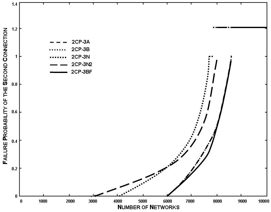
Figure 7: Comparison of algorithms for Problem 2CP-3.

In Figure 7, we consider Problem 2CP-3 and indicate the distribution of the failure probabilities of the second connection obtained after the simulations PL12 for the different algorithms exposed above. Only 10.000 random power-law networks have been generated for the network topology PL12 and none for PL100 because of the excessive computation time due to Algorithm 2CP-3BF. When an algorithm finds a feasible solution, the failure probability of the second connection is, obviously, under $1.0$. If no feasible solution are found, we arbitrarily chose the value of this probability to be equal to $1.2$ to be able to draw it on Figure 7. Since the four source-destination nodes are chosen randomly, in many occasions the two requests do not interfere. This lack of interference is expected to quickly diminish if the number of connections raises. Table II shows the performance (i.e. the proportion of times a minimal value is returned) for Algorithms 2CP-3BF, 2CP-3A 2CP-3B, 2CP-3N and 2CP-3N2 for the network topology PL12.

Network	2CP-3BF	2CP-3A	2CP-3B	2CP-3N	2CP-3N2
PL12	100 %	96.9 %	96.8 %	66.7 %	74.5 %

TABLE II: A second comparison of the algorithms for Problem 2CP-3.

V-C Discussion

Consider first the simulations related to Problem 2CP-2. We observe that the difference in efficiency between Algorithms 2CP-2A and 2CP-2N does not decrease with the increase of the network size. Indeed, despite its increase, the network remains sufficiently sparse to create interference between both connections. Furthermore, we observe that Algorithm 2CP-2A is particulary efficient since in most cases it returns paths with the same (optimal) quality obtained by Algorithm 2CP-2BF.

Similar observations can be derived for Problem 2CP-3. Indeed, all the algorithms are relatively efficient, finding in most cases the optimal value returned by Algorithm 2CP-3BF. In addition, we note that there is only a small difference between the efficiency of 2CP-3A and 2CP-3B, as well as between 2CP-3N and 2CP-3N2. It means that in the fist step of the algorithm, establishing only the primary path $p_{1}$ or also the backup path $b_{1}$ in the same step does not substantially altere the performance of the algorithms. Conversely, the efficiency of the interference minimization and also of our choice of the weight function is visible. Indeed, Algorithms 2CP-3A and 2CP-3B outperform Algorithms 2CP-3N and 2CP-3N2, and almost always returns optimal solutions (i.e., with a minimal failure probability for the second connection).

VI Concluding Remarks

This study analyzed the computational complexity of establishing multiple connections in survivable networks. For several problem variants, optimal solutions of acceptable computational complexity have been established. Other variants have been shown to be computationally intractable, and heuristic schemes, based on the analysis of the respective problems, have been proposed.

This study has been motivated by the fact that, in previous work, only single-connection problems have led to optimal (and computationally efficient) solutions. Our study started with the basic, but yet already complex case where two connections should be established. A differentiation was done between online and offline frameworks, and between fully reliable and unreliable connections.

We then extended our analysis for a fixed $K$ connection problem, where each connection is $100\%$ reliable. For online and offline variants, optimal solutions of polynomial complexity have been established. The intractability of some extensions of the problem was shown.

While this study covered only several out of the many variants of the problem of establishing multiple survivable connections, we believe that its methodical analysis provides a starting point for the rigorous exploration of this important class of problems.

VII Appendix

In the Appendix, we will first prove the intractability of both a variant problem of 2CP when the first connection is already established and is not required to be fully reliable, and of the two disjoint path with forbidden link problem as well. We then prove the tractability of the $K$ connection problem with shared backups, focusing on the restricted case $K=2$ and then enlarging the result. In addition, we prove the intractability of Problem 2CP when an additional bandwidth constraint is added. Then we study the potential restrictions for Problem 2CP. At last, we proceed to characterize the transitions with zero and one leaps.

VII-A Problem 2CP for an Unreliable First Connection

Definition 11

Given a primary path $p_{1}$ and a backup path $b_{1}$ for the first connection $c_{1}$ with possibly some superposition between the two paths, Problem 2CP-u is the problem of finding paths $p_{2}$ and $b_{2}$ for the second connection that minimize their failure probability.

The first connection is not required in Problem 2CP-u to be fully reliable, hence $MCFP(c_{1})$ may be larger than zero and the paths of $c_{1}$ are not necessarily link-disjoint. As we shall show, this problem is NP complete, and, moreover, it is NP-hard even to approximate the solution within a constant factor. The minimization of the failure probability of the second connection is:

$$\min_{p_{2},b_{2}} P_{f}(p_{2}\cap b_{2})+1_{b_{1}\cap p_{2}\neq\oslash,b_{1}\cap b_{2}\neq\oslash}\cdot P_{f}(p_{1}-b_{1})$$

$$+1_{b_{1}\cap b_{2}=\oslash,b_{1}\cap p_{2}\neq\oslash,p_{1}\cap b_{2}\neq\oslash}\cdot P_{f}(p_{1}\cap b_{2})$$

$$s.t. p_{1}\cap p_{2}=\oslash\$$ (9)

Theorem 9

Problem 2CP-u is NP-hard.

Proof: We prove that, given the paths of the first connection, determining if there is a feasible second connection that admits a connection failure probability equal to zero is already NP-hard. We reduce Problem 2CP-u to the two link-disjoint path with forbidden link problem (Problem 2DPFL), which is proven in the next section to be NP-hard. Given a graph $G=(V,E)$ with two nodes $s$ and $t$ in $V,$ and a set $F=\{(u_{1},v_{1}),..,(u_{k},v_{k})\}$ of forbidden links with $F\subseteq E$, Problem 2DPFL requires to determine if there exist two link-disjoint paths from $s$ to $t$ such that at the most one of them is composed of links of $F$.

We consider an instance $(G,s,t,F)$ (same notations as above) of Problem 2DPFL. From this instance we construct an instance $(G^{\prime},s_{1},t_{1},s_{2},t_{2},p_{1},b_{1})$ of Problem 2CP-u such that $G^{\prime}=(V,^{\prime},E^{\prime})$ with $V^{\prime}=V$ and $E^{\prime}=E\cup\{(s,u_{1}),(u_{l},v_{l}),(v_{k},t),1\leq l\leq k\}\cup\{(v_{k},u_{k+1}),1\leq l\leq k-1\}$ (multiple links are accepted in our model) and a uniform weight distribution ($\forall e\in E,P_{f}(e)=\frac{1}{m}$). We also fix $s_{1}=s_{2}=s$ and $t_{1}=t_{2}=t$. The path $s-u_{1}-v_{1}..u_{k}-v_{k}-t$ is chosen as primary path $p_{1}$, and the path $s-u_{1}-v_{1}..u_{k}-v_{k}-t$ corresponds to the backup path $b_{1}$. However, the links $(u_{l},v_{l})$ present in both paths are chosen different. In order to get a zero failure probability for the second connection, only the shared backup case should be considered. Indeed, the other two cases have necessarily a positive failure probability for the second connection, including either the failure probability of $p_{1}$ (the unavoidable first backup case) or the failure probability of $p_{2}$ (the overlapped connection case). Thus, in the shared backup case, the second connection should be composed of link-disjoint paths such that only one path (i.e. $b_{2}$ but not $p_{2}$) may have common links with $b_{1}$ and none of them with $p_{1}$. By construction, the problem precisely corresponds to finding in $G$ two link-disjoint paths such that only one of them may use links in $F$ (composed of links in $b_{1}$ not used by $p_{1}$) and with $s=s_{2}$ and $t=t_{2}$.

Conversely, any solution to the 2DPFL problem where the links of $p_{1}$ have been removed and the remaining links of $b_{1}$ correspond to the forbidden links, is an optimal solution to Problem 2CP-u, since in such a solution the failure probability of the second connection is equal to zero.  

VII-B The Two Disjoint Path with Forbidden Link Problem

Definition 12

Given an undirected graph $G=(V,E)$, two nodes $s$ and $t$ in $V$ and a link subset $F\subseteq E$ (called the forbidden link set), the two link-disjoint path with forbidden link problem (termed 2DPFL) corresponds to finding two link-disjoint paths from $s$ to $t$ such that at least one path includes no links in $F$. In its weighted version, to each link $e\in E$ is assigned a length $l_{e}$, and the weighted two link-disjoint path with forbidden link problem (termed weighted-2DPFL) corresponds to finding two link-disjoint paths from $s$ to $t$ such that at least one path includes no links in $F$ and such that the total length (the sum of the two path lengths) is minimized.

The same problems accept a nodal version, where the disjoint paths should be node disjoint, and the forbidden set is a node set in $V$. The respective problems are called the two node disjoint path with forbidden node problem (termed 2DPFN) and the weighted two node disjoint path with forbidden node problem (termed weighted-2DPFN).

Theorem 10

Problem 2DPFN is NP-complete.

Proof: We show that there is a reduction to Problem 2DPFN from Problem SP-DPFN2 within a polynomial number of steps. We remind to the reader that in Problem SP-DPFN2, given an undirected graph $G=(V,E)$, two nodes $s$ and $t$, and a collection of disjoint forbidden pairs of nodes $W=\{(x_{1},y_{1}),..,(x_{l},y_{l})\}$ such that each node has a degree equal to two, Problem SP-DPFN2 consists in finding a path from $s$ to $t$ that contains at the most one node of each pair. This problem has been proved to be NP-Hard and even Min-PB (see [3]).

We proceed to the reduction in the following way. We take an instance $(G,s,t,W)$ of Problem SP-DPFN2, and we consider all the $r$ links outgoing from $W$ ($r\leq 2l$). We replace the links $W_{e}=\{(w_{1}^{i},w_{2}^{i}),1\leq i\leq r\}$ by adding a new intermediary node $u^{i}$ in each link, getting the link set $U_{e}=\{(w_{1}^{i},u^{i})\cup(u^{i},w_{2}^{i}),1\leq i\leq r\}$. We define $U$ by $U=\{u^{1},..,u^{r}\}$. Then we add a new node set $V_{1}=\{v_{1},..,v_{l+1}\}$ and the link set $F_{1}=\{(s,v_{1}),(v_{i},x_{i}),(v_{i},y_{i}),(x_{i},v_{i+1}),(y_{i},v_{i+1}),(v_{l+1},t),1\leq i\leq l\}$.

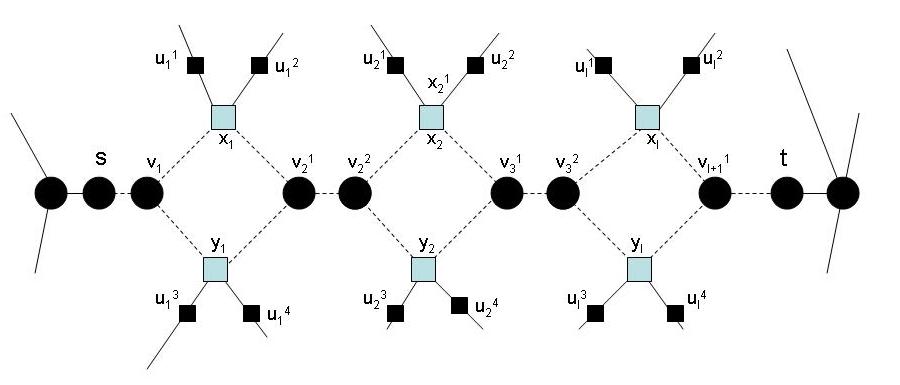
Figure 8: The reduction from SP-DPFN2 to 2DPFN.

Figure 8 depicts the obtained graph (for a better clarity, the links of $G$ have not been drawn except the outgoing links of $W$). Thus we have created a new instance to Problem 2DPFN within a polynomial number of steps: the instance $(G^{\prime},s^{\prime},t^{\prime},F^{\prime})$ is composed of a graph $G^{\prime}=(V^{\prime},E^{\prime})$, such that $V^{\prime}=V\cup U\cup V_{1}$ and $E^{\prime}=(E-W_{e})\cup U_{e}\cup F_{1}$, and a forbidden node set $F^{\prime}=(V-W)\cup U$. The source and the destination are the same (i.e. $s^{\prime}=s$ and $t^{\prime}=t$).

From any solution to Problem 2DPFN with the previous instance we can construct a solution to Problem SP-DPFN2. Indeed, we can (easily) verify that the feasible paths from $s$ to $t$ which have no nodes in $F^{\prime}$ are only those of the form $(s,v_{1},z_{1},v_{2},...,v_{l},z_{l},v_{l+1},t)$ where $z_{i}\in\{x_{i},y_{i}\},1\leq i\leq l$. Thus the other path is in fact a path from $s$ to $t$, without any node of $V_{1}$ and any link of $F_{1}$, and with at the most one node from each disjoint forbidden pair of nodes of $W$. We can find an immediate correspondence between this path and a solution in $G=(V,E)$ to Problem SP-DPFN2.

Conversely, if we have a solution to Problem SP-DPFN2 in $G=(V,E)$, we can construct a path from $s$ to $t$ in $G^{\prime}$ such that none of its nodes is in $F^{\prime}$. Then we can use for the other path the path $(s,v_{1},z_{1},v_{2},...,v_{l},z_{l},v_{l+1},t)$ such that $z_{i}\in\{x_{i},y_{i}\},1\leq i\leq l$. For each forbidden pair of nodes $(x_{i},y_{i})$, $z_{i}$ is either the node not included in the first path (there is always at least one since the first path is built from a solution of SP-DPFN2), or $x_{i}$ if both are not included. These two node disjoint paths represent a feasible solution to Problem 2DPFN.  

Corollary 1

The 2DPFL problem is NP-complete.

Proof: The outline of the proof for the link version of the problem follows the same lines. We consider an instance of the Problem SP-DPFN2 in order to find a linear reduction from it to Problem 2DPFL. We split each node (of degree two) $z\in W$ into two nodes, $z^{1}$ and $z^{2}$, such that each one is only an endpoint of the two previous outgoing links from $z$ (if before the transformation, we had two links $(z,u)$ and $(z,v)$, we have now two links $(z_{1},u)$ and $(z_{2},v)$). In addition, we add the link set $Z_{e}=\{(x_{i}^{1},x_{i}^{2}),(y_{i}^{1},y_{i}^{2}),1\leq i\leq l\}$, the node set $V_{1}$ and the link set $F_{1}$ as defined in the previous proof. We let the reader verify that in this way a valid reduction has been built, and that this reduction can be done in polynomial time.  

Corollary 2

Problem weighted-2DPFL is NP-complete and cannot be approximated within a constant factor.

Proof: As proved in [3], Problem SP-DPFN2 is Min PB complete, which implies that it admits no approximation algorithm within a constant factor. Thus, with the same previous reduction where the link weights of the added links are equal to zero (otherwise they are uniformly equal), we can deduce that the weighted-2DPFL problem is also Min-PB complete, hence does not accept an approximation algorithm within a constant factor.  

VII-C The $K$ Connection Problem with Shared Backups

Definition 13

Given an undirected graph $G=(V,E)$ and $K$ pairs of nodes ($s_{1}$,$t_{1}$),..,($s_{K}$,$t_{K}$) in $V$, The $K$ connection establishment with shared backup path problem (termed K-CESB) consists in finding $2K$ paths $\{p_{1},b_{1},..,p_{K},b_{K}\}$ connecting their corresponding source-destination pair such that no link can be common to different paths except if they are all backup paths.

For example, for $K=2$, Problem 2-CESB consists in finding four paths $p_{1},b_{1},p_{2}$ and $b_{2}$ connecting their corresponding source-destination pair such that all pair of paths are link disjoint except the two backup paths that may have common links.

Theorem 11

Problem 2-CESB can be resolved in a polynomial time.

Proof: We will show that an algorithm that solves a four, five and seven link-disjoint path problem solves Problem 2-CESB. Since finding four, five or seven link-disjoint paths can be solved by the polynomial time algorithm presented in [21], Problem 2-CESB can be also solved in a polynomial time (we observe however that the algorithm in [21] needs a unrealistic computation time for determining constants). We focus first on the case where two of the four special nodes $\{s_{1},s_{2},t_{1},t_{2}\}$ are identical, let assume $s_{1}=s_{2}=s$. If a solution exists, we can built another solution that follows one this two compositions: either four link-disjoint paths to the destinations (no superposition between the backup paths) or three link-disjoint paths to the destination and an additional link-disjoint path from one of the backup path to the destination (when backup shared common links). In this last composition, the backup paths share a first partial path and then use different links to get to their respective destination.

In the second composition, if the backup paths share common links (but not necessarily continuously) a feasible solution can be composed by recomposing one of the backup path as follows. If we denote by $x$ the last node shared by both backup paths before getting to their respective destination, the partial path between $s$ and $x$ of the backup path $b_{2}$ can be modified such that it uses all the links used by the other backup path $b_{1}$ until $x$. This solution is also feasible since there is no overlap with any primary paths. In order to verify the existence of a solution in this case where $s_{1}=s_{2}$, we can verify the existence of four link disjoint paths to the destinations by linking each of them twice to an fictitious node and to run a flow algorithm (first composition). For the other composition, we verify the existence of five link disjoint paths (from $s$ to $t_{1}$, from $s$ to $t_{2}$, from $s$ to $x$, from $x$ to $t_{1}$ and from $x$ to $t_{2}$) by running an algorithm that solves the five link-disjoint path problem, testing it for all $x\in V-\{s_{1},s_{2},t_{1},t_{2}\}$. If any solution exists, the algorithm returns a solution and conversely, any solution returned by the algorithm solves Problem 2-CESB.

We assume here that the four special nodes $s_{1},s_{2},t_{1}$ and $t_{2}$ are distinct. By a similar analysis, if a solution exists, two compositions for a solution are relevant: either four link-disjoint paths from their respective source to their respective destination, or seven link-disjoint paths (from $s_{1}$ to $t_{1}$, from $s_{2}$ to $t_{2}$, from $s_{1}$ to $x$, from $s_{2}$ to $x$, from $x$ to $y$, from $y$ to $t_{1}$ and from $y$ to $t_{2}$) where $x$ and $y$ are distinct regular nodes, as depicted in Figure 9

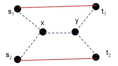
Figure 9: The second composition in Problem 2-CESB.

(we observe moreover that we can interchange $s_{2}$ and $t_{2}$ since the graph is undirected). Indeed, if the backup paths in the original solution have no common links, it corresponds to the first composition. On the contrary, if some links are shared, we call $x$ and $y$ the first and last nodes shared by $b_{2}$ with $b_{1}$ in its way to $t_{2}$. We can replace the partial path of the original second backup path $b_{2}$ between $x$ and $y$ by the links of $b_{1}$ in order to get a feasible solution which corresponds to the second composition previously described. The first composition can be solved by an algorithm solving the four link-disjoint path problem, and the second composition by an algorithm solving the seven link disjoint path problem.

In all the previous compositions, a solution is returned by the algorithm if the instance is solvable, and if an algorithm finds a solution, it corresponds effectively to a solution for Problem 2-CESB.  

Theorem 12

For a bounded $K$, Problem K-CESB can be resolved in a polynomial time.

Proof: We have previously seen the proof for $K=2$. In that proof, we have seen that an algorithm solving the $l$ link-disjoint path problem, for $1\leq l\leq 7$, suffices to solve Problem K-CESB for $K=2$. In this proof, we will generalize it to an algorithm solving the $l$ link-disjoint path problem, for $1\leq l\leq 5K-3$. We proceed by strong induction. The property we aim to prove is formulated as follows: for a bounded $K$, Problem K-CESB can be solved with the help of an algorithm solving the $l$ link-disjoint path problem, for $1\leq l\leq 5K-3$. The initialization step is already verified for $K=1$ and $K=2$.

Let assume that for all $1\leq i\leq K-1$ the property is true for $i$ and we want to prove that the property is also true for $K$. We claim that if a solution exists, then a relevant solution can be found such that it has one of the two following composition: either a solution with a disconnected backup subgraph (the subgraph composed of all the backup paths) such that each connected component corresponds to a case already seen, or a connected backup subgraph such that all the backup paths are included in it and this subgraph can be represented by a tree composed at the most of $5K-3$ branches.

We consider a solution to the K-CESB problem and we build the backup graph. If the graph is connected, we want to show that an algorithm solving the $l$ link-disjoint path problem, for $1\leq l\leq 5K-3$, solves our problem. Since all the paths are entirely included in this connected backup graph, it necessarily includes all the special nodes $\{s_{1},t_{1},..,s_{K},t_{K}\}$. From this connected graph, we can remove links in order to build a tree that links all these special nodes such that all the leaves of this tree will be only special nodes. We consider the number of branches of this tree: in the worst case, all the special nodes are leaves which are linked to the trunk through distinct nodes. In the worst case, the number of nodes in the tree is $2K+(2K-2)=4K-2$, and the number of branches is $4K-3$. Thus, in order to verify if such a tree exists, we should verify all the possible combinations for the number of internal nodes (from $1$ to $2K-2$), and all the combinations from these nodes to the special nodes, such that each special node is linked to exactly one of these nodes. In other words, we verify the possibility of any tree as described above by fixing only the internal nodes with a degree superior to three. In addition, in these verifications, we always work under the constraint that additional $K$ link-disjoint primary paths connects their respective source-destination pair. In the worst case, we will have to find these $K$ primary paths and the $4K-3$ other paths composing the described tree.

If the graph is disconnected, it means that we can find at least two backup paths such that it is impossible to go from a node of a path to a node of the other path only through backup links (links used in this solution by backup paths). In fact, each connected component is composed of some backup paths, such that each backup path is located to exactly one connected component. We proceed in a similar way (by constructing a tree in each connected component). As a consequence, we can verify if such a solution exists by considering all the possible partitions of backup paths and all the possible combinations for each connected component. For each possibility, the number of link-disjoint paths to consider for a tree of a component including $j$ backup paths is less than $4j-3$. Thus, the total number of link-disjoint paths to consider will be also bounded here by $5K-3$, which verifies the property for $K$. We underline here that all the considered configurations can be easily verified by the reader as representing a feasible solution if they exist.

In addition, the total number of combinations $N$ we consider remains polynomial in $n$. Indeed, we can express an upper bound by:

$$N \leq \sum_{m=1}^{K}\sum_{i_{1}\geq..\geq i_{m},s.t.\sum_{l=1}^{m}i_{l}=K}\frac{K!}{\prod_{l=1}^{m}i_{l}!}.\prod_{i_{j}\neq 1,j=1}^{m}\left[\sum_{x=2}^{2i_{j}-2}{n\choose x}x^{2i_{j}}\right]$$ (10)

$$\leq K.2^{K}.n^{2K}.(2K-2)^{2K}\$$

We conclude that $N$ is polynomial in $n$. Thus, the algorithm solving Problem K-CESB verifies these $N$ combinations. If a solutions exists, the algorithm returns a feasible solution. Conversely, any solution returns by the algorithm solves Problem K-CESB.  

Theorem 13

For a fixed $K$, Problem OffKCP can be solved within a polynomial number of steps.

Proof: Problem OffKCP is equivalent by its definition to Problem K-CESB, which is proven above (Theorem 12) to be solvable within a polynomial number of steps.  

Theorem 14

For an unfixed $K$, Problem K-CESB is NP-hard.

Proof: A simple reduction to the general link-disjoint path problem, which is NP-hard as proven amongst the “classic” NP-Hard problems in [12] can be done. Considering an instance $(G,s_{1},t_{1},..,s_{K},t_{K})$ of Problem K-CESB with $G=(V,E)$, and the special nodes $\{(s_{1},t_{1}),..,(s_{K},t_{K})\}$ in $V$, with $K$ not necessarily bounded, we construct for the general link-disjoint path problem the following instance. We add two nodes, $x$ and $y$, and $2K+1$ links, linking $x$ to all the sources, $y$ to all the destinations, and $x$ to $y$. This reduction can be done within a polynomial number of steps. On one hand, an algorithm that would solve Problem K-CESB would solve the general link-disjoint path problem by taking the additional links as part of the shared backup paths. Conversely, from any solution of the general link-disjoint path problem we can construct a solution to this modified instance for the problem.  

Theorem 15

For a general (not $O(1)$) $K$, Problem KCP is NP-complete. Moreover, it is NP-hard to approximate it within a constant factor.

Proof: Consider an instance $(G,s_{1},t_{1},..,s_{K},t_{K})$ of Problem KCP, such that $G=(V,E)$ is an undirected uniformly weighted graph and $\{(s_{i},t_{i}),1\leq i\leq K\}$ are the source-destination pairs of the $K$ connections. We consider Problem KCP when all the connections are required to be perfectly reliable (i.e. $MCFP(c_{1})=..=MCFP(c_{K})=0$). Thus, only the shared backup case can be applied. For this instance, Problem KCP is equivalent to Problem K-CESB, which is proven above to be NP-Hard and, moreover, it is NP-hard to approximate it within a constant factor.  

VII-D Problem KCP with a Bandwidth Constraint

We proceed to establish the intractability of Problem OKCP in the presence of bandwidth constraints. Even with this bandwidth constraint, the primary (resp. backup) path of a new connection request is not allowed to use links already used by a previous primary or backup (resp. primary) paths. In addition, similarly to [14], the routing does not tolerate traffic splitting.

Definition 14

For an instance $I=(G,s_{k},t_{k},b_{k})$, where $G=(V,E)$ is a weighted undirected graph, we define the weight $b_{e}$ of link $e$ as composed of three parameters $(b_{1}(e),b_{2}(e)b_{3}(e))$, such that $b_{1}(e)$, $b_{2}(e)$ and $b_{3}(e)$ respectively correspond to the bandwidth taken by the previous primary paths, by the previous backup paths and the available bandwidth on the link. The capacity $c(e)$ of link $e$ is: $c(e)=b_{1}(e)+b_{2}(e)+b_{3}(e)$. $(s_{K},t_{K})$ are two nodes of $V$, $b_{k}$ is the bandwidth demand of the request, and we call the bandwidth online $K$ connection problem (in short, BW-OKCP) the problem of finding two link-disjoint paths from $s_{K}$ to $t_{K}$ (“primary” and “backup”) such that the primary (resp. backup) path is allowed to use only links with a first and second (resp. first) bandwidth parameter equal to zero and a third parameter (resp. the sum of the second and the third parameters) superior to $b_{k}$.

Theorem 16

Problem BW-OKCP is NP-complete.

Proof: We prove that we can reduce Problem BW-OKCP to Problem 2-DPFL, which is proven above (Theorem 1) to be NP-complete.

We consider an instance $(G,s_{K},t_{K},b_{k})$ of Problem BW-OKCP. We call $G_{1}$ the restricted graph of links $e$ of $G$ such that $b_{1}(e)=0$. These links are not used by any previous primary paths. We assume that all the links $e$ of $G_{1}$ such that $b_{2}(e)=0$ have a third parameter $b_{3}(e)>b_{K}$. In addition, we assume that amongst the links $e$ of $G_{1}$ with $b_{2}(e)>0$, some links may not have enough bandwidth $c(e)<b_{k}$, while others may have. We call $G_{2}$ the graph resulting from the removal of the links without enough bandwidth from $G_{1}$. Thus, Problem BW-OKCP is reduced for this instance to Problem 2-DPFL, with the instance $(G^{\prime},s^{\prime},t^{\prime},F^{\prime})$ such that $G^{\prime}=G_{2}$, $s^{\prime}=s_{k}$, $t^{\prime}=t_{k}$ and the forbidden link set $F^{\prime}$ is equal to the set of links in $G_{2}$ with a strictly positive second parameter. Indeed, Problem BW-OKCP exactly corresponds in finding two link-disjoint paths from $s^{\prime}$ to $t^{\prime}$ in $G^{\prime}$ such that only the backup path is allowed to use links of $F^{\prime}$.  

VII-E The Study of Potential Restrictions for Problem 2CP

We analyze here the different cases for Problem 2CP. Except common links between $p_{1}$ and $p_{2}$, we consider all the eight combinations whether we allow superposition between $b_{1}$ and $b_{2}$, $b_{1}$ and $p_{2}$, or $p_{1}$ and $b_{2}$. We analyze the different schemes in order to observe if some are superfluous. The following table sums up the different cases, where only the first three cases are necessary (Table III).

Overlapping	($p_{1}$,$b_{2}$)	($b_{1}$,$p_{2}$)	($p_{2}$,$b_{2}$)
The shared backup case	X	X	X,V
The unavoidable first backup case	X	V	V
The overlapped connection case	V	V	X
The fourth case	V	V	V
The fifth case	X	V	X
The sixth backup case	V	X	X
The seventh backup case	V	X	V

TABLE III: Comparison of the different cases for Problem 2CP.

We detail the features of each case. The first case corresponds to the shared backup case, when only $b_{2}$ (or $p_{2}$ in the symmetric fifth case) can have superposition with $b_{1}$, and no one with $p_{1}$. We have already seen above that if $p_{1}$ is fixed, and there is a feasible solution to this case, then it is the optimal one. The second case is the unavoidable first backup case, where both paths of the second connection have a superposition with $b_{1}$, and none with $p_{1}$.

The third case is, like the second case, an interesting one only when the first case has no feasible solution and then it may be better than the second case; it has been called the overlapped connection case.

The next cases (from the fourth to the seventh one) can always be improved by previous cases and are thus not relevant. In the fourth case, we take into account both additions in the optimization expression and get as a goal the minimization of $P_{f}(p_{2})+P_{f}(p_{1})$. We show that this fourth case cannot outperform the unavoidable first backup case. If $p_{1}$ is fixed for example, we get the same value in the unavoidable first backup case by taking the shortest path for $p_{2}=b_{2}$, and any path for $b_{1}$ ($b_{1}$ may have superposition with $p_{2}$ and $b_{2}$). The general case is also reachable by the unavoidable first backup case by adopting the same primary path $p_{1}$.

The fifth case has been showed to be equivalent to the shared backup case. The sixth and the seventh cases can be improved by the shared backup case. Since $p_{2}$ has no superposition with $p_{1}$ and $b_{1}$, only if its links fail then the second connection automatically fails. The optimization corresponds to the minimization of $P_{f}(p_{2})$. We can reach the same value by taking $b_{2}=p_{2}$ in the shared backup case: then $b_{2}$ has no superposition with $p_{1}$ and $b_{1}$, and we minimize the same expression.

VII-F The Two link-disjoint Path Problem and its Extension

Definition 15

We call the two link path problem (termed TPP) the problem of finding for an instance $I=(G,s_{1},s_{2},t_{1},t_{2})$, where $G$ is an undirected graph and $(s_{1},s_{2},t_{1},t_{2})$ are four nodes of this graph, two link-disjoint paths respectively from $s_{1}$ to $t_{1}$ and from $s_{2}$ to $t_{2}$.

We present here the theorem as stated in [7] that completely characterizes the solvability of Problem TPP for a two-link connected graph. The proof can be found in [24].

Theorem 17

Let $G$ be a graph such that no cut link separates both of the two terminal pairs $(s_{1},t_{1})$ and $(s_{2},t_{2})$. There is no two link-disjoint paths between the corresponding terminal pairs if and only if some links of $G$ can be contracted so that the resulting graph $G^{\prime}$ is planar, the four terminals have degree two while the other nodes are of degree three, and the terminal are positioned on the outer face in this order: $s_{1},s_{2},t_{1},t_{2}$.

References

- [1] R. Banner and A. Orda. “The power of tuning: a novel approach for the efficient design of survivable networks”. In IEEE/ACM Transactions on Networking, 15 (4): 737-749, 2007.
- [2] R. Bhandari. “Survivable Networks Algorithms for Diverse Routing”. Kluwer, 1999.
- [3] R. Bhatia, M. Kodialam and T.V. Lakshman. “Finding disjoint paths with related path costs”. In Journal of Combinatorial Optimization, 12: 83-96, 2006.
- [4] E. W. Dijkstra. “A Note on Two Problems in Connection with Graphs”. In Num. Mathematik, 1:269 -271, 1959.
- [5] M. Faloutsos, P. Faloutsos and C. Faloutsos. “On Power-Law Relationships of the Internet Topology”. In Proc. SIGCOMM, 215-262, 1999.
- [6] S. Fortune, J.E. Hopcroft and J. Wyllie. “The Directed Subgraph Homeomorphism Problem”. In Th. Computer Science 10: 111-121, 1980.
- [7] A. Frank. “Packing Paths, Circuits, and Cuts - a Survey”. In Paths, Flows, and VLSI Layout, B. Korte, L. Lovasz, H. Promel and A. Schrijver, Eds., Berlin: Sprnger-Verlag, 1990.
- [8] A. Fumagalli and M. Tacca. “Optimal Design of Optical Ring Networks with DiR”. In Lecture Notes In C.S., 1989: 299-314, 2001.
- [9] W. D. Grover. “Mesh-Based Survivable Transport Networks: Options and Strategies for Optical, MPLS, SONET and ATM Networking”. Prentice-Hall, 2003.
- [10] P. Ho, J. Tapolcai and H. Mouftah. “Diverse Routing for Shared Protection in Survivable Optical Networks”. In Proc. of IEEE Globecom 2003, 5: 2519-2523, 2003.
- [11] V. Kann. Polynomially bounded minimization problems that are hard to approximate, Nordic Journal of Computing, 1 (3), 317-331, 1994.
- [12] R. Karp. “Reducibility among combinatorial problems”. In Complexity of Computer Computation, R. Miller and al., Plenum Press, 85-103, 1972.
- [13] M. Kodialam and T.V. Lakshman. “Dynamic Routing of Bandwidth Guaranteed Tunnels with Restoration”. In IEEE Infocom, 902-911, 2000.
- [14] M. Kodialam and T.V. Lakshman. “Minimum Interference Routing of Bandwidth Guaranteed Tunnels with MPLS Traffic Engineering Applications”. In J. on Sel. Areas on Comm., 18 (12): 2566-2579, 2000.
- [15] G. Li, B. Doverspike and C. Kalmanek. “Fiber Span Failure Protection in Mesh Optical Networks”. In Proc. of SPIE, 4599: 130-141, 2001.
- [16] G. Maier, A. Pattavina, S. De Patre and M. Martinelli. “Optical Network Survivability: Protection Techniques in the WDM layer”. In Photonic Network Communication, 4 (3): 251-269, 2002.
- [17] J. Marzo, E. Calle, C. Scoglio and T. Anjali. “QoS Online Routing and MPLS Multilevel Protection: a Survey”. In IEEE Comm. Mag., 2003.
- [18] K. Menger. “Zur allgemeinen Kurventheorie”. In Fundamental Mathematics, 19: 96-115, 1927.
- [19] H. Nagamochi, K. Nishimura and T. Ibaraki. “Computing all small cuts in undirected networks”. In SIAM J. Discrete Math., 10: 469 -481, 1997.
- [20] B. Reed, N. Robertson, A. Schrijver and P. Seymour. “Finding disjoint trees in planar graph in linear time”. In Contemporary Math., 147:295 -301, 1993.
- [21] N. Robertson and P. Seymour. “Outline of a disjoint paths algorithm”. In Paths, Flows, and VLSI Layout, B. Korte and al, Springer-Verlag, 1990.
- [22] J. W. Suurballe and R. Tarjan. “A Quick Method for Finding Shortest Pairs of Disjoint Paths”. In Networks, 14: 325-336, 1984.
- [23] T. Tholey. “Solving the 2-disjoint paths problem in nearly linear time”. In Theory of Computing Systems, 39 (1): 51-78, 2006.
- [24] C. Thomassen. “2-linked graphs”. In Preprint Series 1979/80, No. 17, Mathematisk Institut, Aarhus Universitet, 1979.
- [25] S. Zhou. “Understanding the evolution dynamics of internet topology”. In Physical Review, 74 (016- 124), 2006.