Multipulse storage and manipulation via solitonic solutions

Abstract

Solutions to the Maxwell-Bloch equations for a $\Lambda$ system are computed using the single-soliton Darboux transformation and the nonlinear superposition principle. These allow complete control of information deposited by a signal pulse (with the help of an auxiliary control pulse) in the coherence of the medium’s ground states by injecting sub-sequential pulses. Additionally, we study the encoding of two signal pulses and their manipulation by a control pulse and show that multipulse storage and control are possible as long as the imprints made by encoding the signal pulses are sufficiently separated.

I Introduction

The observation of a solitary canal wave by Scott Russell in 1834 is considered the historical origin of soliton studies, but the enormous growth of the field began more than a century later. This is due to the discovery of new methods for solving the nonlinear equations that describe them, such as inverse scattering gardner1967method ; ablowitz1973nonlinear ; lamb1980elements , the Bäcklund transformation lamb1971analytical ; miura1976backlund and the Darboux transformation gu2006darboux ; cieslinski2009algebraic , to name a few. This phenomenon has been increasingly studied in several fields of physics, and particularly in optics kivshar2003optical . McCall and Hahn were the first to observe these solitary optical waves, as reported in their famous papers mccall1967self ; mccall1969self where they introduced the concept of self-induced transparency (SIT). Due to the coherent interaction of the pulses with the medium, they can propagate without attenuation. This is the shape-preserving property of solitons that is sometimes used to define them. McCall and Hahn also found that the optical pulses tailor their intensity profile so that the total pulse area, defined in terms if the Rabi frequency [see Eqs. (4)] as

$$\theta(x)=\int^{\infty}_{-\infty}\Omega(x,t)dt,$$ (1)

tends towards the closest even multiple of $\pi$. This is the very well-known area theorem, which is a consequence of the smoothing effects of Doppler broadening allen2012optical .

Quantum optical systems have always been envisioned as the ideal candidates for building reliable quantum memories. This is due to their small decoherence and short interaction times milonni2004fast . Many procedures have achieved light manipulation grobe1994formation and storage. Light can be slowed down to the point where its information is encoded in the medium fleischhauer2000dark ; turukhin2001observation and then retrieved as was shown in liu2001observation . Some other techniques such as a combination of electromagnetic-induced transparency (EIT) and four-wave mixing vudyasetu2008storage ; camacho2009four have been shown to work. The downside of these sorts of procedures is that they rely on a slow resonant light-atom interaction that is characteristic of EIT harris1997electromagnetically ; boller1991observation . If this interaction is instead led by short pulses, we can open the door to high-speed control and manipulation of light.

The regime of broadband pulses interacting with matter leads to new possibilities for light control. The interaction of strong electromagnetic fields with atomic systems is described by nonlinear evolution equations (which are hard to solve) and the use of numerical computation is usually required. In some special circumstances, they become integrable and thus solvable by the methods previously mentioned. In the particular case of a $\Lambda$ system (see Fig. 1), the Maxwell-Bloch equations that define the evolution of the system become integrable when both signal and control fields have equal atom-field coupling parameters and are in two-photon resonance, as has been shown by Park and Shin park1998matched and Clader and Eberly clader2007two . This leads to solitonic solutions even in non-ideal media preparation such as “mixonium” clader2008two , a partially coherent medium. Other studies have been carried out for the case of ultra-cold atoms, where one can neglect the effects of Doppler broadening and homogeneous relaxation. Given these assumptions, Groves et al. deduced a second order solution that led to an alternative scheme for storage and manipulation of light groves2013jaynes . Complementary numerical simulations gutierrez2015manipulation showed the relevance of this procedure even under the effects of the ever-present spontaneous emission. Here we continue this work by presenting new solutions that allow full control of the information stored in the ground state elements of the density matrix. We present the generalization to multiple pulse storage as well as a three-step control by the corresponding computation of higher order solutions.

II Theoretical framework

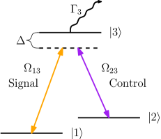
Figure 1: Three level atom in $\Lambda$ configuration, with spontaneous emission $\Gamma_{3}$ from the excited state interacting with two fields in two-photon resonance.

We consider the interaction of strong short pulses with a $\Lambda$ system in two-photon resonance with each field tuned to address a different atomic transition. The atomic dipole operator is taken to be $\boldsymbol{d}=\boldsymbol{d}_{13}\left|1\right>\left<3\right|+\boldsymbol{d}_{23}\left|2\right>\left<3\right|+\boldsymbol{d}_{31}\left|3\right>\left<1\right|+\boldsymbol{d}_{32}\left|3\right>\left<2\right|$, thus only linking levels 1 to 3 and 2 to 3. As is customary, the fields are written in carrier-envelope form:

$$\boldsymbol{E}(x,t)= \boldsymbol{\mathcal{E}}_{13}(x,t)e^{i(k_{13}x-\omega_{13}t)}$$

$$+\boldsymbol{\mathcal{E}}_{23}(x,t)e^{i(k_{23}x-\omega_{23}t)}+c.c$$ (2)

where $\omega_{13}$ and $\omega_{23}$ are the field frequencies, $k_{13}$ and $k_{23}$ are the vacuum wave numbers and $\boldsymbol{\mathcal{E}}_{13}(x,t)$ and $\boldsymbol{\mathcal{E}}_{23}(x,t)$ are the slowly-varying field envelopes. We assume that the pulses are short enough so that we can neglect the effects of spontaneous emission but long enough so that the envelopes change slowly over many cycles of the optical frequency, thus justifying the slow-varying envelope approximation (SVEA). Following groves2013jaynes we refer to the 1-3 field as the signal pulse and the 2-3 field as the control pulse. Abandoning the bare frequencies in favor of the common detuning, the total Hamiltonian in the rotating wave approximation (RWA) takes the form:

$$H=-\frac{\hbar}{2}\left(\begin{array}[]{ccc}0&0&\Omega_{13}^{*}\\ 0&0&\Omega_{23}^{*}\\ \Omega_{13}&\Omega_{23}&-2\Delta\end{array}\right)$$ (3)

where we defined the Rabi frequencies,

$$\Omega_{13}(x,t) =2\boldsymbol{d}_{31}\cdot\boldsymbol{\mathcal{E}}_{13}(x,t)/\hbar,$$ (4a)

and

$$\Omega_{23}(x,t) =2\boldsymbol{d}_{32}\cdot\boldsymbol{\mathcal{E}}_{23}(x,t)/\hbar,$$ (4b)

and the detuning $\Delta=(E_{3}-E_{1})/\hbar-\omega_{13}=(E_{3}-E_{2})/\hbar-\omega_{23}$ (here $E_{i}$ denotes the energy of level $\left|i\right>$). The atomic system evolves according to the von Neumann equation for the density matrix:

$$i\hbar\frac{\partial\rho}{\partial t}=[H,\rho]$$ (5)

and the fields follow Maxwell’s wave equation in the SVEA:

$$\left(\frac{\partial}{\partial x}+\frac{1}{c}\frac{\partial}{\partial t}\right)\Omega_{13} =i\mu_{13}\rho_{31}$$ (6a)

and

$$\left(\frac{\partial}{\partial x}+\frac{1}{c}\frac{\partial}{\partial t}\right)\Omega_{23} =i\mu_{23}\rho_{32}.$$ (6b)

Here, we defined the atom-field coupling parameters $\mu_{j3}=N\omega_{j3}|d_{j3}|^{2}/\hbar\epsilon_{0}c$ with $j=1,\,2$. This gives us a set of eight nonlinear partial differential equations that need to be solved simultaneously. As stated previously, we need to consider the special case of two-photon resonance and equal atom-field coupling parameters, $\mu_{13}=\mu_{23}=\mu$. This way we can use the methods described in the introduction. In the travelling-wave coordinates $T=t-x/c$ and $Z=x$, Eqs. (5) and (6) take the form:

$$i\hbar\frac{\partial\rho}{\partial T}=[H,\rho]$$ (7a)

and

$$\frac{\partial H}{\partial Z}=-\frac{\hbar\mu}{2}[W,\rho],$$ (7b)

where the constant matrix

$$W=i\left|3\right>\left<3\right|=\left(\begin{array}[]{ccc}0&0&0\\ 0&0&0\\ 0&0&i\end{array}\right)$$ (8)

has been introduced. By combining these two equations it is easily shown that the Lax equation,

$$\partial_{Z}U-\partial_{T}V+[U,V]=0,$$ (9)

is satisfied where the Lax operators are defined as $U=-(i/\hbar)H-\lambda W$ and $V=(i\mu/2\lambda)\rho$, and $\lambda$ is a constant known as the spectral parameter. This effectively shows that the Maxwell-Bloch equations [Eqs. (7b)] are integrable.

Throughout this framework, we have only considered the longitudinal spatial dimension; this was justified by the assumption of plane waves. In reality, the pulses will have a nonuniform intensity profile that will inevitably lead to deviation from the theoretical assumption by effects such as pulse stripping, diffraction and self-focusing mccall1969self . To mitigate this we can use pulses that have a coherent frequency profile, have their bandwidth determined only by the finite extent of their envelope, and are free of chirping. Additionally, an aperture can be used to ensure a planar wavefront and homogeneous distribution of intensity. An example of this can be seen in the beautiful experiments on SIT by Gibbs and Slusher gibbs1970peak ; slusher1972self . Another thing worth mentioning is that the finite extent of the pulses imposes some restrictions in the use of atomic beams to get rid of Doppler broadening, namely, the transit time broadening must be smaller than the bandwidth of the pulses. This must be satisfied in order to ensure that the atoms where the signal pulse was encoded are the same that are interacting with the subsequent pulses.

III Solution method

III.1 Darboux transformation

Figure 2: Bianchi diagram for the theorem of permutability. By requiring commutativity of the diagram we are able to find an algebraic method to compute higher order solutions.

The basic idea of the Darboux transformation is to start from a system of partial differential equations of the form:

$$\frac{\partial\psi}{\partial T}=U\psi\quad\text{and}\quad\frac{\partial\psi}{\partial Z}=V\psi,$$ (10)

then consider a transformation $\bar{\psi}=D\psi$ so that

$$\frac{\partial\bar{\psi}}{\partial T}=\bar{U}\bar{\psi}\quad\text{and}\quad\frac{\partial\bar{\psi}}{\partial Z}=\bar{V}\bar{\psi},$$ (11)

where

$$\bar{U}=DUD^{-1}+(\partial_{T}D)D^{-1}$$ (12a)

and

$$\bar{V}=DVD^{-1}+(\partial_{Z}D)D^{-1}.$$ (12b)

Now we want to construct the operator $D$ in terms of known parameters such as the original solution to the linear Eq. (10). We also want it to preserve the spectral dependence of the Lax pair, in which case we call it a Darboux matrix. Additionally, we need to conserve the hermiticity of the density matrix and Hamiltonian which in turn requires that $U(\lambda)^{\dagger}=-U(\lambda^{*})$ and $V(\lambda)^{\dagger}=-V(\lambda^{*})$. Such Lax operators belong to what is known as the unitary reduction. Starting from the “single-soliton” Darboux matrix, we have that

$$D=(\lambda-\lambda_{1})I-(\lambda_{1}-\lambda_{1}^{*})P$$ (13)

in order to satisfy all the required properties (cieslinski2009algebraic, ), where $I$ is the identity matrix and $P$ is a hermitian projection operator ($P^{2}=P$ and $P=P^{\dagger}$). Taking $\lambda_{1}$ to be complex leads to more complicated solutions and so we will consider it to be purely imaginary, thus getting

$$D=\lambda I+\lambda_{1}(2P-I).$$ (14)

From the previous section we know that the Lax operators for the Maxwell-Bloch equations [Eqs. (7b)] have the following spectral dependence:

$$U(\lambda) =\lambda^{0}U_{0}+\lambda^{1}U_{1}$$ (15a)

$$V(\lambda) =\lambda^{-1}V_{-1}.$$ (15b)

After inserting this into Eqs. (12) and collecting terms of equal order in $\lambda$ we find:

$$\lambda^{0}: \quad\bar{U}_{0}M=MU_{0}+\partial_{T}M$$ (16a)

$$\lambda^{1}: \quad\bar{U}_{0}+\lambda_{1}\bar{U}_{1}M=U_{0}+\lambda_{1}MU_{1}$$ (16b)

$$\lambda^{2}: \quad\bar{U}_{1}=U_{1}$$ (16c)

and

$$\lambda^{-1}: \quad\bar{V}_{-1}M=MV_{-1}$$ (17a)

$$\lambda^{0}: \quad\bar{V}_{-1}=V_{-1}+\lambda_{1}\partial_{Z}M$$ (17b)

where we defined the unitary involution $M=2P-I$. It is worth noting that from Eq. (16c) it is clear that the matrix $W$ will remain constant between solutions, as it should. Writing the projection operator as $P=\left|\varphi\right>\left<\varphi\right|/\left<\varphi\vphantom{\varphi}\right|\left.\varphi\vphantom{\varphi}\right>$ it is possible to use Eqs. (16) and (17) to determine a set of equations for the column vector $\left|\varphi\right>$. By means of the properties of the projection operator, the result can be simplified to obtain a set of two linear differential equations that determine $\left|\varphi\right>$:

$$\left(I\partial_{T}-U(-\lambda_{1})\right)\left|\varphi\right>=0,$$ (18a)

$$\left(I\partial_{Z}-V(-\lambda_{1})\right)\left|\varphi\right>=0.$$ (18b)

This derivation is similar to the one presented by Clader and Eberly in clader2007two . Solving Eqs. (18) determines the projection operator and thus the Darboux matrix.

From the definition of the Lax operators for the Maxwell-Bloch equations we can relate the new solution to the first order density matrix and Hamiltonian. If we assume that our seed solution was given by the density matrix $\rho^{0}$ and the Hamiltonian $H^{0}$, it follows that

$$H=H^{0}-i\hbar\lambda_{1}\left[M,W\right],$$ (19a)

$$\rho=M\rho^{0}M.$$ (19b)

III.2 Nonlinear superposition rule

In principle, the method described in the previous section could be used to compute higher order solutions, but the reality is that Eqs. (18) become harder to solve with each step. Luckily there is a much simpler way to achieve this: the theorem of permutability (Fig. 2). Starting from a seed solution (zeroth order) $U^{0}$ and $V^{0}$, it is possible to construct two new solutions $U^{a}$ and $V^{a}$ with the associated parameter $\lambda_{a}$ and $U^{b}$, and $V^{b}$ with associated parameter $\lambda_{b}$ using the Darboux matrices $D^{a}$ and $D^{b}$ that are of the form given by Eq. (14). From these first order solutions we can construct second order solutions by applying $D^{ab}$ with parameter $\lambda_{b}$ to the $a$ solution and $D^{ba}$ with parameter $\lambda_{a}$ to the $b$ solution thus obtaining the new pairs of Lax operators $U^{ab}$ $V^{ab}$ and $V^{ba}$ $U^{ba}$. The theorem of permutability asserts that there is nothing special about the order in which the second order solutions are computed. This is equivalent to requiring commutativity of the Bianchi diagram as shown in Fig. 2. Both second order solutions should then be the same, $U^{ab}=U^{ba}$ and $V^{ab}=V^{ba}$.

Using Eqs. (16) and (17) for the second order Lax pair and setting the result from the two paths equal to each other, we can derive the following expression for the second order involution matrix:

$$M^{ab}=(\lambda_{a}M^{a}-\lambda_{b}M^{b})(\lambda_{a}M^{a}M^{b}-\lambda_{b}I)^{-1}.$$ (20)

It is easy to relate this to the density matrix and Hamiltonian, thus bypassing the need to compute the Darboux matrix and solve complicated differential equations. Using the properties of the involution matrices it is easy to show that

$$\rho^{ab}=M^{ab}M^{a}\rho^{0}M^{a}M^{ab}$$ (21a)

and

$$H^{ab}=H^{0}-i\hbar(\lambda_{a}^{2}-\lambda_{b}^{2})\left[(\lambda_{a}M^{a}-\lambda_{b}M^{b}),W\right].$$ (21b)

This treatment can be extended to obtain third order solutions by purely algebraic methods. Once more we assume the commutativity of the Bianchi diagram up to the third order which, again, is a statement of the independence of the path taken from a total of six possibilities (see Fig. 2). After some simplifications using the properties of the involution matrices and the solution for the second order, the expression for the third order involution matrix can be written in similar form as the one for the second order, namely:

$$M^{abc}=(\lambda_{b}M^{ab}-\lambda_{c}M^{ac})(\lambda_{b}M^{ab}M^{ac}-\lambda_{c}I)^{-1}.$$ (22)

This is the same as using the nonlinear superposition rule [Eq. (20)] on two second order solutions. Finally, relating this result to the density matrix and Hamiltonian we have

$$\rho^{abc}=M^{abc}M^{ab}M^{a}\rho^{0}M^{a}M^{ab}M^{abc}$$ (23a)

and

$$H^{abc}=H^{a}-i\hbar(\lambda_{b}^{2}-\lambda_{c}^{2})\left[(\lambda_{b}M^{ab}-\lambda_{c}M^{ac}),W\right].$$ (23b)

Table 1: Elements of the involution matrix $M^{a}$ for the three types of first order solutions considered.

	Type 1 ($a_{1},a_{2},a_{3}\neq 0$)		Type 2 ($a_{1}=0$)	Type 3 ($a_{2}=0$)
	$T/\tau_{a}\ll-1$	$T/\tau_{a}\gg 1$	for all times	for all times
$M_{11}^{a}$	$\tanh\left(\frac{T}{\tau_{a}}-\frac{\mu\tau_{a}}{2}Z+\eta_{13}^{a}\right)$	$\tanh\left(-\frac{\mu\tau_{a}}{2}Z+\eta_{12}^{a}\right)$	$-1$	$\tanh\left(\frac{T}{\tau_{a}}-\frac{\mu\tau_{a}}{2}Z+\eta_{13}^{a}\right)$
$M_{22}^{a}$	$-1$	$-\tanh\left(-\frac{\mu\tau_{a}}{2}Z+\eta_{12}^{a}\right)$	$\tanh\left(\frac{T}{\tau_{a}}+\eta_{23}^{a}\right)$	$-1$
$M_{33}^{a}$	$-\tanh\left(\frac{T}{\tau_{a}}-\frac{\mu\tau_{a}}{2}Z+\eta_{13}^{a}\right)$	$-1$	$-\tanh\left(\frac{T}{\tau_{a}}+\eta_{23}^{a}\right)$	$-\tanh\left(\frac{T}{\tau_{a}}-\frac{\mu\tau_{a}}{2}Z+\eta_{13}^{a}\right)$
$M_{12}^{a}$	$0$	$A_{12}\text{sech}\left(-\frac{\mu\tau_{a}}{2}Z+\eta_{12}^{a}\right)$	$0$	$0$
$M_{13}^{a}$	$A_{13}\text{sech}\left(\frac{T}{\tau_{a}}-\frac{\mu\tau_{a}}{2}Z+\eta_{13}^{a}\right)$	$0$	$0$	$A_{13}\text{sech}\left(\frac{T}{\tau_{a}}-\frac{\mu\tau_{a}}{2}Z+\eta_{13}^{a}\right)$
$M_{23}^{a}$	$0$	$A_{23}\text{sech}\left(\frac{T}{\tau_{a}}+\eta_{23}^{a}\right)$	$A_{23}\text{sech}\left(\frac{T}{\tau_{a}}+\eta_{23}^{a}\right)$	$0$

IV First order solutions

After reviewing the solution method, we now proceed to solve the Maxwell-Bloch equations [Eqs. (7b)]. For simplicity we will consider the special case of zero detuning. The seed is taken to be the trivial solution of a quiescent medium ($\rho^{0}=\left|1\right>\left<1\right|$) and no fields ($\Omega_{13}=\Omega_{23}=0$), so that $H^{0}=0$. It is easy to see that by solving Eqs. (18)

$$\left|\varphi^{a}\right>=\left(\begin{array}[]{c}a_{1}e^{-\mu\tau_{a}Z/2}\\ a_{2}\\ a_{3}e^{-T/\tau_{a}}\end{array}\right),$$ (24)

where $a_{1}$, $a_{2}$, $a_{3}$ are constants of integration. Here, we wrote the Darboux parameter as $\lambda_{a}=i/\tau_{a}$, with $\tau_{a}\in\mathbb{R}$ which makes it easier to associate it to a physical quantity, namely, the duration of the pulses. Two possible solutions arising from this have already been thoroughly studied by Groves, Clader and Eberly (groves2013jaynes, ) so we will just summarize the results that we will need. Table 1 contains all the elements of the involution $M^{a}$ for the three first order solutions that are going to be considered.

The most general solution (type 1) is given by taking all the integration constants to be different from zero. In this case we end up with a special case of the two-pulse soliton solution previously found by Clader and Eberly in (clader2007two, ). In the limit $t/\tau_{a}\ll-1$ we have a SIT-like signal pulse propagating, driving population from the ground state $\left|1\right>$ into the excited state $\left|3\right>$ and coherently driving it back, thus obtaining the characteristic SIT $2\pi$-pulse shaped as an hyperbolic secant. As the control pulse is only zero in the limit of infinite negative time, some of the excited population is coherently driven into the ground state $\left|2\right>$, thus amplifying the seed of the control pulse. Its effect slowly takes over, up to the point where the signal pulse starts to be depleted as the control pulse is amplified [see Fig. 3(a)].

During this transfer the signal pulse encodes its information into the ground state elements $\rho_{11}$, $\rho_{22}$ and $\rho_{12}$ of the density matrix. Table 1 only shows the elements of the matrix $M^{a}$ at infinite positive and negative times as these can be written in a simple form and are the most relevant information. From these and Eq. (19b) the shape of the ground state elements of the density matrix can be obtained and are given by:

$$\rho_{11}^{a}=\tanh^{2}\left(-\frac{\mu\tau_{a}}{2}Z+\eta_{12}^{a}\right),$$ (25a)

$$\rho_{12}^{a}=A_{12}\text{sech}\left(-\frac{\mu\tau_{a}}{2}Z+\eta_{12}^{a}\right)\tanh\left(-\frac{\mu\tau_{a}}{2}Z+\eta_{12}^{a}\right),$$ (25b)

$$\rho_{22}^{a}=\text{sech}^{2}\left(-\frac{\mu\tau_{a}}{2}Z+\eta_{12}^{a}\right).$$ (25c)

All other elements of $\rho^{a}$ are zero. The location of the imprint is where the population of state $\left|2\right>$ has a maximum (this also corresponds with the minimum of $\rho_{11}^{a}$ and the zero of $\rho_{12}^{a}$) and thus is given by

$$\kappa_{a}x_{1}^{a}=\eta^{a}_{12},$$ (26)

where $\kappa_{a}=\mu\tau_{a}/2$ is the absorption coefficient in the absence of Doppler broadening. An example of this imprint is depicted by the plots with continuous lines in Fig. 4.

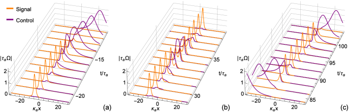
Figure 3: Third order solution for a single imprint obtained from the nonlinear superposition of a first order solution of each type: (a) shows the initial encoding of the signal pulse at $\kappa_{a}x_{1}=0$, (b) shows the collision of a second signal pulse with the imprint which displaces it to $\kappa_{a}x_{1}=-5$ and (c) shows the collision of the imprint with a control pulse which moves it to $\kappa_{a}x_{1}=5$. The corresponding imprints are depicted in Fig. 4.

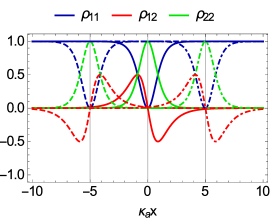
Figure 4: Information encoding and control in a $\Lambda$ system: Imprint as it has been encoded in the ground state density matrix elements after the initial encoding (continuous line), after the first backward displacement (dashed lines) and after the second forward displacement (dot-dashed lines). The imprint was generated and displaced by the pulse sequence depicted in Fig. 3 and the snapshots were taken at times $t/\tau_{a}=0$, $60$ and $150$, respectively.

The addition of Doppler broadening would affect the definition of the absorption coefficient and thus change the group velocity of the pulses in the medium, but the encoding would still carry through. It is also worth noting that while the two pulses are active, the area of the individual pulses is no longer equal to $2\pi$ but the total pulse area as defined in (clader2007two, ),

$$\theta_{\text{tot}}=\sqrt{|\theta_{13}|^{2}+|\theta_{23}|^{2}},$$ (27)

remains constant and equal to $2\pi$. After the storage process is over, $t/\tau_{a}\gg 1$, we have a $2\pi$-control pulse propagating away at the speed of light as it is decoupled from the medium. Both signal and control pulses have a duration of $\tau_{a}$ and are time-matched.

Another possibility is taking one of the integration constants to be zero. If $a_{1}=0$ then we obtain a type 2 solution which is a $2\pi$-control pulse traveling at the speed of light completely decoupled from the medium. If instead we take $a_{2}=0$ we end up with an SIT solution for the signal pulse which we will refer to as type 3. This pulse propagates at a reduced group velocity, coherently driving population from state $\left|1\right>$ to the excited state $\left|3\right>$ and back again, thus keeping its hyperbolic secant shape as it propagates.

V Single imprint manipulation

V.1 Backward-transfer solution

Now we make use of the nonlinear superposition rule [Eq. (20)] to combine a type 1 solution with a type 3 solution, to which we assign the letters $a$ and $b$ respectively. The parameters $\eta_{jk}$ defined in Table 1 did not have any relevance other than to control where the signal pulse deposited its information into the medium for the type 1 solutions. Now that we are superimposing two first order solutions it acquires renewed relevance as it also controls the order of the pulses and whether the type 1 pulse has enough time to make the imprint before the type 3 pulse collides with it. The Rabi frequencies in the limit of infinitely negative time are given by

$$\Omega_{13}^{ab}= -\frac{2i}{\tau_{a}}A_{13}^{*}\text{sech}\left(\frac{T}{\tau_{a}}-\frac{\mu\tau_{a}}{2}Z+\eta_{13}^{a}+\delta^{ab}\right)$$

$$+\frac{2i}{\tau_{b}}B_{13}^{*}\text{sech}\left(\frac{T}{\tau_{b}}-\frac{\mu\tau_{b}}{2}Z+\eta_{13}^{b}-\delta^{ab}\right),$$ (28a)

$$\Omega_{23}^{ab}=0,$$ (28b)

where we defined the phase lag parameter

$$\delta^{ab}=\ln\left|\frac{\tau_{a}+\tau_{b}}{\tau_{a}-\tau_{b}}\right|.$$ (29)

Here, we will stick to the case where $\eta_{13}^{a}\gg\eta_{13}^{b}$ to guarantee that the signal pulse from the type 1 solution has enough time to encode its information into the medium before the second signal pulse collides with it.

From the type 1 solution, we have that the first signal pulse will imprint its information at a location determined by Eq. (26). This proceeds as the already described type 1 first order solution, and the corresponding pulse dynamics are shown in Fig. 3(a). Then comes the second signal pulse of different duration $\tau_{b}$. As it approaches the imprint, the second signal pulse starts to decay as it gives way to a control pulse, which mediates the transfer of the peak of the signal pulse from the new location of the imprint to where it was first made. Therefore the imprint is effectively pushed backwards. Finally, the control pulse decays and the signal pulse continues to propagate as an SIT-type solution. This process is shown in Fig. 3(b). This effect is clearly due to the long tails of the sech-shaped pulses that can sense changes in the medium long before the peak of the pulses and thus interact with it accordingly. This is similar to what happens with fast light, where the long tails of the pulse sense the inverted medium and so the peak of the pulse is displaced at a speed greater than that of light due to stimulated emission wang2000gain ; boyd2002slow ; clader2006coherent ; clader2007theoretical .

In order to determine what the effect was on the imprint, we need to compute the ground state elements of the density matrix in the limit of infinitely positive long time using Eq. (21a). We find that

$$\rho_{11}^{ab}=\tanh^{2}\left(-\frac{\mu\tau_{a}}{2}Z+\eta_{12}^{a}-\delta^{ab}\right),$$ (30a)

$$\rho_{12}^{ab}= -\phi A_{12}\text{sech}\left(-\frac{\mu\tau_{a}}{2}Z+\eta_{12}^{a}-\delta^{ab}\right)$$

$$\times\tanh\left(-\frac{\mu\tau_{a}}{2}Z+\eta_{12}^{a}-\delta^{ab}\right),$$ (30b)

$$\rho_{22}^{ab}=\text{sech}^{2}\left(-\frac{\mu\tau_{a}}{2}Z+\eta_{12}^{a}-\delta^{ab}\right),$$ (30c)

where $\phi=\text{sgn}(\tau_{a}-\tau_{b})$ which determines the phase of the coherence.

The effect is clear: The imprint is displaced to the left by an amount determined by the phase lag parameter with a possible phase shift in the coherence $\rho_{12}$ depending on the relation between the duration of the pulses. The dashed line plots in Fig. 4 show the displaced imprint. This is the same result as the one obtained when superimposing a type 1 and a type 2 first order solution except that the sign of the displacement is inverted, and so the imprint is moved to the right. This has already been shown in groves2013jaynes ; gutierrez2015manipulation .

V.2 Multi-step manipulation

Having identified all the relevant parameters in the control of a single imprint by studying the second order solutions, we can proceed to extend this control to multi-step processes. Here we consider only third order solutions which are composed of three steps. The first will be the imprinting step, then we can consider a combination of other control and/or signal pulses to move the imprint back and forth.

For clarity lets consider the case of pushing the imprint to the left and then to the right by means of type 3 and type 2 first order solutions, respectively. We compute the third order solution by means of the superposition rule given by Eq. (22). This situation is depicted in Fig. 3 where each frame corresponds to a step and each will be labelled by their corresponding letters $a$, $b$ and $c$. First, the information of the initial signal pulse of duration $\tau_{a}$ is deposited in the form of an imprint that is made into the medium as determined by Eq. (26). Then comes a second signal pulse of duration $\tau_{b}$. Its effect is the same as described in the previous section. The imprint is moved to the left and its new location is $\kappa_{a}x_{2}^{a}=\kappa_{a}x_{1}^{a}-\delta^{ab}$. As has already been mentioned, there is a phase shift in the coherence $\rho_{12}$ if $\tau_{b}<\tau_{a}$. Finally, for the third step, a control pulse of duration $\tau_{c}$ comes in. Upon interaction with the imprint, it reads the information stored and retrieves the initial signal pulse which, in turn, is restored in a new location given by $\kappa_{a}x_{3}^{a}=\kappa_{a}x_{2}^{a}+\delta^{ac}$ with the same possibility for another $\pi$-phase shift for $\rho_{12}$. The results of creation and displacements of the imprint are shown in Fig. 4. Continuous lines show the first imprinted density matrix elements, dashed lines represent the first displacement to the left and dot-dashed lines show the imprint when it is displaced to the right.

It should be clear that the generalization for single imprint manipulation to an n${}^{\text{th}}$ order solution follows from the previous results. We can readily write the final location of the imprint,

$$\kappa_{a}x_{n}^{a}=\eta_{12}^{a}-\sum_{i=1}^{m_{2}}\delta^{ab_{i}}+\sum_{i=1}^{m_{3}}\delta^{ac_{i}},$$ (31)

where $m_{2}$ and $m_{3}$ are, respectively, the number of type 2 and 3 first order solutions that compose this n${}^{\text{th}}$ order solution. Additionally, if there is an odd number of pulses with duration shorter than $\tau_{a}$ (the original signal pulse) then there is a $\pi$-phase shift for the imprint.

VI Multiple imprint control

VI.1 Two imprints solution

The first step to generalize this control to multiple imprint dynamics is to study the second order solution born out of the superposition of two type 1 solutions. This will simulate the scenario of having two signal pulses each with their own control pulse seed. As each pair of pulses have different time duration, one of them will be traveling faster. The parameters have to be carefully chosen so that the first signal pulse, which we will label with the letter $a$, deposits its information into the medium before the second, labeled with the letter $b$, catches up. In the limit of infinite negative time the Rabi frequencies are given the same expressions as for the backward-transfer solution Eqs. (28). Therefore, in order to have the correct order for the pulses, the condition $\eta_{13}^{a}\gg\eta_{13}^{b}$ must be satisfied.

Here again, after the first pair of pulses of time duration $\tau_{a}$ has deposited the information of the signal pulse, the density matrix elements are given by Eqs. (25) and the location of the first imprint $x_{1}^{a}$ is determined by Eq. (26). When the second imprint is made, if we want to preserve the information of each pulse separately, we need to have that $|\eta_{12}^{a}-\eta_{12}^{b}|\gg 1$. Using this and the expressions given in Table 1 in the infinite time limit, we can work out expressions for the density matrix elements around each imprint. In the vicinity of the first imprint (the one made by the pulses of duration $\tau_{a}$) we have:

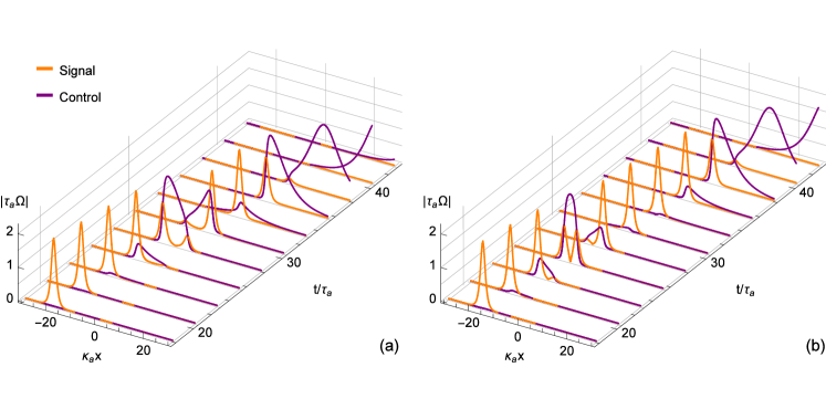
Figure 5: Encoding of a second signal pulse. (a) A signal pulse of duration $\tau_{a}$ was encoded at $\kappa_{a}x_{1}^{a}=\eta_{12}^{a}$ and then comes a second signal pulse of duration $\tau_{b}$ meant to be stored at $\kappa x_{1}^{b}=\eta_{12}^{b}$, with $x_{1}^{a}>x_{1}^{b}$. (b) Here the reverse process is presented, the pulse $\tau_{b}$ is the first to be encoded and the pulse $\tau_{a}$ is the second. The values for the $\eta_{12}$’s are kept the same as well as those of the $\tau$’s. Both cases lead to the same imprint which is shown in Fig. 6.

$$\rho_{11}^{ab}=\tanh^{2}\left(-\frac{\mu\tau_{a}}{2}Z+\eta_{12}^{a}+\sigma\delta^{ab}\right),$$ (32a)

$$\rho_{12}^{ab}= -\phi A_{12}\text{sech}\left(-\frac{\mu\tau_{a}}{2}Z+\eta_{12}^{a}+\sigma\delta^{ab}\right)$$

$$\times\tanh\left(-\frac{\mu\tau_{a}}{2}Z+\eta_{12}^{a}+\sigma\delta^{ab}\right),$$ (32b)

$$\rho_{22}^{ab}=\text{sech}^{2}\left(-\frac{\mu\tau_{a}}{2}Z+\eta_{12}^{a}+\sigma\delta^{ab}\right),$$ (32c)

where we defined $\sigma=\text{sgn}(\eta_{12}^{a}-\eta_{12}^{b})$. Around the second imprint we have similar expressions with the signs in front of $\sigma$ and $\phi$ reversed.

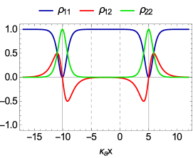
Figure 6: Multi-pulse storage in a $\Lambda$-system: Each imprint made by the storage of two signal pulses of duration $\tau_{a}$ and $\tau_{b}$. The vertical continuous lines show the location of each imprint and the dashed ones show where they would have been encoded if they had been by themselves.

There are several things to comment about these expressions but the most obvious and somewhat shocking is that the parameters $\eta_{13}^{a}$ and $\eta_{13}^{b}$ are nowhere to be found. This means that the temporal order in which the imprints were made is irrelevant; the only thing that matters is the spatial ordering as it is shown by the dependence on $\eta_{12}^{a}$ and $\eta_{12}^{b}$. Therefore the two processes depicted in Fig. 5 lead to the same result. On one hand, we have the situation assumed here, namely, that the signal pulse $\tau_{a}$ stores its information first and $x_{1}^{a}>x_{1}^{b}$. When the second signal pulse $\tau_{b}$ is coming in, it senses the presence of the first imprint and thus “knows” that it must deposit its information before the value predicted by Eq. (26). This again is clearly a feature of the long tails of the sech-shaped pulses that start interacting with the imprint long before the peak collides with it. The information is then encoded in a process similar to the one described by a type 1 first order solution. The control pulse that comes out from the encoding process then pushes the first imprint in a way similar to the prediction from a superposition of type 1 and 2 first order solutions. This process is shown in Fig. 5(a). Now, on the other hand, we have the situation where the signal pulse $\tau_{b}$ encodes its information into the medium first. Then comes the second signal pulse $\tau_{a}$. When it comes close to the imprint it acts as a backward-transfer solution, thus displacing the imprint by the amount discussed in Sec. V.1. Then, it continues its propagation but, due to the translation it suffered while displacing the first imprint, it encodes its information into a displaced location. This complicated pulse dynamic is displayed in Fig. 5(b).

Regardless of which situation took place, the location of the two imprints is now given by,

$$\kappa_{a}x_{2}^{a} =\eta_{12}^{a}+\sigma\delta^{ab},$$ (33a)

$$\kappa_{b}x_{2}^{b} =\eta_{12}^{b}-\sigma\delta^{ab}.$$ (33b)

An example of the resulting imprints after the two pulses have stored their information is presented in Fig. 6. The vertical dashed lines show the predicted location given by Eq. (26): These would be the actual locations of each imprint if they were done separately.

VI.2 Simultaneous imprint control

Now that we have demonstrated that the encoding of two signal pulses is possible and have quantified the effect on each imprint due to the presence of the other, we need to address the question of multi-imprint control. To do this we consider the concrete example of pushing the imprints made by the two imprint solution discussed in the previous section via a control pulse of duration $\tau_{c}$. We compute this third order solution by means of the superposition rule [Eq. (22)]. The resulting pulse dynamics for the displacement step are shown in Fig. 7. As the control pulse comes in, it first encounters the imprint made by the signal pulse $\tau_{b}$. Consequent to the interaction the signal pulse is retrieved, which in turn causes it to propagate and start encoding its information back into the medium. The storage gives way to another control pulse which immediately starts interacting with the imprint left by the signal pulse $\tau_{a}$. This signal pulse is then retrieved, it propagates and finally is re-encoded into the medium at a displaced location giving way to a control pulse that propagates away at the speed of light.

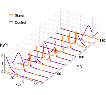
Figure 7: Displacement step of the third order solution computed from the superposition of two type 1 and a type 2 first order solutions. The resulting imprints are depicted in Fig. 8.

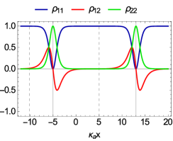
Figure 8: Imprints displaced by a control pulse of duration such that $\tau_{a}>\tau_{c}>\tau_{b}$. The vertical continuous lines give the location of the imprints and the dashed ones show their previous location. These correspond to the pulse dynamics presented in Fig. 7.

Figure 8 shows the displaced imprint: The vertical dashed lines represent the location of each imprint before collision with the control pulse. There we can clearly see that each imprint was displaced a different amount and that just one of them suffered a $\pi$-phase shift. Each imprint is displaced according to their own parameters, that is, the new location for the $\tau_{a}$ imprint is

$$\kappa_{a}x_{3}^{a}=\kappa_{a}x_{2}^{a}+\delta^{ac}$$ (34)

and for the $\tau_{b}$ imprint we have

$$\kappa_{b}x_{3}^{b}=\kappa_{b}x_{2}^{b}+\delta^{bc}.$$ (35)

As we considered the case $\tau_{a}>\tau_{c}>\tau_{b}$ for plotting Figs. 7 and 8, following the results previously stated, we get that only the imprint with larger duration suffers the $\pi$-phase shift. Therefore we have shown that the manipulation of multiple imprints follows the single imprint rules as long as one respects the spatial limits of each imprint. That means that the control pulse should not push the first imprint it encounters beyond the second one. This does not imply that it cannot be done, just that the end result for the imprints is going to be different. From everything that has been said so far it is not hard to say what would happen in this scenario. When the control pulse collides with the first imprint it retrieves the signal pulse stored. This signal pulse then encounters the second imprint and thus interacts with it as a backward-transfer solution displacing the imprint to the left. Finally the signal pulse encodes its information, thus effectively inverting the order of the imprints.

If instead of moving the imprints with a control pulse we had chosen a type 3 first order solution then everything would have been reversed. The imprints would be moved to the left according to the results derived in Sec. V.1. Here again, there is an option for inverting the order of the imprints. If the duration of the type 3 pulse is tailored so that the imprint on the right is displaced more that the separation between imprints plus their widths, then the order is reversed. Each imprint would be moved in a different direction as well: The imprint on the right is displaced to the left by the signal pulse and the imprint on the left is pushed to the right by the control pulse that mediates the backward-transfer.

VII Conclusions

Throughout this manuscript we have shown the usefulness of a solution method via the Darboux transformation and the nonlinear superposition principle for generating sequences of pulses useful for storage and manipulation of information. It can be employed to compute higher order solutions which give rise to complicated sequences of pulses by purely algebraic, albeit tedious, calculations.

The new backward-transfer solution along with the solution presented in (groves2013jaynes, ) allow complete control of the information encoded by a signal pulse in the ground state coherence of the atomic system. The imprint can be moved backward or forward any number of times by means of control and signal pulses. This is particularly important for unidirectional systems where the pulses can only propagate through the atomic medium in one direction, be that by design or experimental necessity. The generation of higher order solutions showed that the control of the imprint can be extended to any number of steps moving the imprint back and forth. In practice this might not be completely true: We will need to abandon the idealized condition of infinitely long pulses and media and consider the effect of decoherence due to spontaneous emission. But as existing numerical experiments show gutierrez2015manipulation , storage and manipulation are still possible with a somewhat different dependence on the different parameters than the analytical solution, and they still present the same trend. Of course the degrading effects of decoherence may limit the number of steps in order to keep a certain degree of fidelity in the information stored. Note that the finiteness of the medium provides a way to retrieve the signal pulse by frustrating its re-encoding by the end face when displaced by a control pulse.

We also showed that multi-pulse storage is possible, and the effects due to the presence of another imprint can be quantified. This study could be continued to analyze the effect of encoding more pulses and see if the locations of the imprints follow a predictable trend from which it would be possible to extrapolate the behavior for any number of imprints. Additionally, we showed that manipulation of the imprints by means of pulses of type 2 and 3 is possible. In this case, there are additional consideration, such as the spatial extent of each imprint. Overlapping the imprints must be avoided when displacing the imprint a long distance or inverting their order. But from the numerical data, there is a maximum displacement that could very well hinder any chance of inverting the imprint or overlapping them (as long as enough room was left between them during the encoding stage) for any realistic experimental scenario.

A final note must be made about the effects of Doppler broadening on the encoding and retrieval of the signal pulse. In Ref. clader2007two Clader and Eberly worked out the first order solution presented here with the added effects of Doppler broadening. From their work we can see that, in the case where the Doppler distribution is centered around resonance, the imprint made on all the atoms is located at the same place but (assuming a real coherence $\rho_{12}$ on resonance) for the atoms off resonance the real part of the ground-state coherence is attenuated and acquires an imaginary part. This imaginary part has a sign that depends on the sign of the detuning, so there will be an equal number of atoms with negative and positive imaginary parts. When taking the average over the Doppler distribution, this contribution will cancel out. Therefore, when a control pulse collides with the imprint, the only consequence is the attenuation of the real part for some atoms which will inevitably hinder the retrieval of the signal pulse but never suppress it completely.

References

- (1) C. S. Gardner, J. M. Greene, M. D. Kruskal, and R. M. Miura, “Method for solving the Korteweg-deVries equation,” Phys. Rev. Lett. 19, 1095–1097 (1967).
- (2) M. J. Ablowitz, D. J. Kaup, A. C. Newell, and H. Segur, “Nonlinear-evolution equations of physical significance,” Phys. Rev. Lett. 31, 125–127 (1973).
- (3) G. L. Lamb, Elements of Soliton Theory (Wiley, New York, 1980).
- (4) G. L. Lamb, “Analytical descriptions of ultrashort optical pulse propagation in a resonant medium,” Rev. Mod. Phys. 43, 99–124 (1971).
- (5) R. M. Miura, Backlund Transformations (Springer-Verlag, Berlin, 1976).
- (6) C. Gu, H. Hu, and Z. Zhou, Darboux Transformations in Integrable Systems (Springer, Dordrecht, 2005).
- (7) J. L. Cieśliński, “Algebraic construction of the Darboux matrix revisited,” J. Phys. A: Math. Theor. 42, 404003 (2009).
- (8) Y. S. Kivshar and G. Agrawal, Optical solitons: from fibers to photonic crystals (Academic, San Diego, 2003).
- (9) S. L. McCall and E. L. Hahn, “Self-induced transparency by pulsed coherent light,” Phys. Rev. Lett. 18, 908–911 (1967).
- (10) S. L. McCall and E. L. Hahn, “Self-induced transparency,” Phys. Rev. 183, 457–485 (1969).
- (11) L. Allen and J. H. Eberly, Optical Resonance and Two-Level Atoms (Dover, New York, 1987).
- (12) P. W. Milonni, Fast Light, Slow Light and Left-Handed Light (Institute of Physics, Bristol, 2005).
- (13) R. Grobe, F. T. Hioe, and J. H. Eberly, “Formation of shape-preserving pulses in a nonlinear adiabatically integrable system,” Phys. Rev. Lett. 73, 3183–3186 (1994).
- (14) M. Fleischhauer and M. D. Lukin, “Dark-state polaritons in electromagnetically induced transparency,” Phys. Rev. Lett. 84, 5094–5097 (2000).
- (15) A. V. Turukhin, V. S. Sudarshanam, M. S. Shahriar, J. A. Musser, B. S. Ham, and P. R. Hemmer, “Observation of ultraslow and stored light pulses in a solid,” Phys. Rev. Lett. 88, 023602 (2001).
- (16) C. Liu, Z. Dutton, C. H. Behroozi, and L. V. Hau, “Observation of coherent optical information storage in an atomic medium using halted light pulses,” Nature (London) 409, 490–493 (2001).
- (17) P. K. Vudyasetu, R. M. Camacho, and J. C. Howell, “Storage and retrieval of multimode transverse images in hot atomic rubidium vapor,” Phys. Rev. Lett. 100, 123903 (2008).
- (18) R. M. Camacho, P. K. Vudyasetu, and J. C. Howell, “Four-wave-mixing stopped light in hot atomic rubidium vapour,” Nature Photonics 3, 103–106 (2009).
- (19) S. E. Harris, “Electromagnetically induced transparency,” Phys. Today 50, 36–42 (1997).
- (20) K.-J. Boller, A. Imamoğlu, and S. E. Harris, “Observation of electromagnetically induced transparency,” Phys. Rev. Lett. 66, 2593–2596 (1991).
- (21) Q. Han Park and H. J. Shin, “Matched pulse propagation in a three-level system,” Phys. Rev. A 57, 4643–4653 (1998).
- (22) B. D. Clader and J. H. Eberly, “Two-pulse propagation in media with quantum-mixed ground states,” Phys. Rev. A 76, 053812 (2007).
- (23) B. D. Clader and J. H. Eberly, “Two-pulse propagation in a partially phase-coherent medium,” Phys. Rev. A 78, 033803 (2008).
- (24) E. Groves, B. D. Clader, and J. H. Eberly, “Jaynes–Cummings theory out of the box,” J. Phys. B: At. Mol. Opt. Phys. 46, 224005 (2013).
- (25) R. Gutiérrez-Cuevas and J. H. Eberly, “Manipulation of optical-pulse-imprinted memory in a system,” Phys. Rev. A, 92, 033804 (2015).
- (26) H. M. Gibbs and R. E. Slusher, “Peak amplification and breakup of a coherent optical pulse in a simple atomic absorber,” Phys. Rev. Lett. 24, 638–641 (1970).
- (27) R. E. Slusher and H. M. Gibbs, “Self-induced transparency in atomic rubidium,” Phys. Rev. A 5, 1634–1659 (1972).
- (28) L. J. Wang, A. Kuzmich, and A. Dogariu, “Gain-assisted superluminal light propagation,” Nature 406, 277–279 (2000).
- (29) R. W. Boyd and D. J. Gauthier, “‘Slow’ and ‘fast’ light,” Prog. Opt. 43, 497–530 (2002).
- (30) B. D. Clader, Q. Han Park, and J. H. Eberly, “Fast light in fully coherent gain media,” Opt. Lett. 31, 2921–2923 (2006).
- (31) B. D. Clader and J. H. Eberly, “Theoretical study of fast light with short sech pulses in coherent gain media,” J. Opt. Soc. Am. B 24, 916–921 (2007).