Multiple Correspondence Analysis & the Multilogit Bilinear Model

Abstract

Multiple Correspondence Analysis (MCA) is a dimension reduction method which plays a large role in the analysis of tables with categorical nominal variables such as survey data. Though it is usually motivated and derived using geometric considerations, in fact we prove that it amounts to a single proximal Newtown step of a natural bilinear exponential family model for categorical data the multinomial logit bilinear model. We compare and contrast the behavior of MCA with that of the model on simulations and discuss new insights on the properties of both exploratory multivariate methods and their cognate models. One main conclusion is that we could recommend to approximate the multilogit model parameters using MCA. Indeed, estimating the parameters of the model is not a trivial task whereas MCA has the great advantage of being easily solved by singular value decomposition and scalable to large data.

keywords: nominal data, dimension reduction, low-rank approximation, latent-space models, contingency table, correspondence analysis.

1 Introduction

Principal component methods such as principal component analysis (PCA), correspondence analysis (CA) (Greenacre, 2007) or multiple correspondence analysis (MCA) (Greenacre and Blasius, 2006) are often used as multivariate descriptive methods to explore and visualize data. They are similar in their main aims but differ with respect to the nature of the data they deal with: principal component analysis for quantitative data, correspondence analysis for contingency tables (crossing two categorical variables) and multiple correspondence analysis for categorical data. These data dimensionality reduction methods allow to study the similarities between rows, similarities between columns, and associations between rows and columns and provide a subspace that best represents the data in the sense of maximizing the variability of the projected points. A great importance is attached to the graphical outputs to shed lights into the results and often the representation of rows is as interesting as the columns one (Husson et al, 2010).

An intrinsic characteristic of the approaches is that they are motivated by geometrical considerations without any reference to probabilistic models, in line with Benzécri (1973)’s idea to “let the data speak for themselves”. From a technical point of view, the core of all these methods is the singular value decomposition (SVD) of certain matrices with specific row and column weights and metrics (used to compute the distances). In the words of Benzécri (1973), “Doing a data analysis, in good mathematics, is simply searching eigenvectors, all the science of it (the art) is just to find the right matrix to diagonalize.”

Even so, specific choices of weights and metrics can be viewed as inducing specific models for the data under analysis. Understanding the connections between exploratory multivariate methods and their cognate models can yield insights into the methods’ properties and offer for instance solutions when explicit models struggle with high dimensional data. Indeed, principal components methods have the great advantage to be easily scalable to large data sets. In addition, it may give new opportunities to common problems for principal components methods such as inference, tests to select the number of components, and missing values.

In this paper, we begin in Section 2 with a brief review of PCA, CA and their cognate models in one place, with a focus on their similarities. We also include a new presentation of CA as a generalized linear model with a data driven link function. Then, we describe in Section 3 the multinomial logit bilinear model to study the structure of dependence between categorical variables and derive theoretical results relating MCA to this model. We show that MCA amounts to a single proximal Newton step on the multilogit model. Finally, in Section 4 we conduct a simulation study to compare and contrast the behavior of the multilogit model with that of MCA and discuss the potential of such new connections.

2 Underlying Models in PCA and in CA

2.1 The Linear-Bilinear Model and PCA

A classical model related to PCA is the fixed-effects model of Caussinus (1986), also known as the fixed factor score model (de Leeuw et al, 1985) and discussed in Allen et al (2014). In that model, the data matrix ${\bf X}\in\mathbb{R}^{n\times m}$ is generated from column effects and a rank-$K$ interaction matrix, corrupted by isotropic Gaussian noise:

$$x_{ij}\sim\mathcal{N}(\mu_{ij},\sigma^{2}),\text{ with }\mu_{ij}=\beta_{j}+\Gamma_{ij},$$ (1)

with the constraint that $\text{rank}(\bm{\Gamma})\leq K$. Equivalently, we can write

$$\mu_{ij}=\beta_{j}+\sum_{k=1}^{K}d_{k}u_{ik}v_{jk},$$

with identifiability constraint ${\bf U}^{T}{\bf U}={\bf V}^{T}{\bf V}={\bf\mathbb{I}}_{K}$. Maximum likelihood estimation of $\bm{\Gamma}$ amounts to least-squares approximation of the column-centered data matrix ${\bf Z}={\left({\bf\mathbb{I}}_{n}-\frac{1}{n}{\mathds{1}}{\mathds{1}}^{T}\right)}{\bf X}$, the matrix of residuals after orthogonalizing with respect to the column effect $\bm{\beta}$. That is, $\bm{\widehat{\Gamma}}$ is simply the rank-$K$ partial singular value decomposition (SVD) ${\bf U}_{K}{\bf D}_{K}{\bf V}_{K}^{T}$, leading to the classical PCA normalized scores ${\bf u}_{i}$ and loadings ${\bf v}_{j}$. The solution can also be obtained using an alternating least squares algorithm (with a multiple regression step to estimate ${\bf U}$ and a multiple regression step to estimate ${\bf V}$).

Model (1) is also called a linear-bilinear model (Mandel, 1969; Denis and Gower, 1994, 1996; Groenen and Koning, 2006), an additive main effects and multiplicative interaction model (AMMI) or a biadditive model (Gabriel, 1978; Gauch, 1988; Gower and Hand, 1995) and is extremely popular in analysis of variance with two factors. In that case one often includes an additive row effect as well:

$$\mu_{ij} =\alpha_{i}+\beta_{j}+\sum_{k=1}^{K}d_{k}u_{ik}v_{jk}$$ (2)

Model (2) is useful to estimate the interaction between the factors when no replication is available.

2.2 The Log-Bilinear Model and CA

Log-linear models (Agresti, 2013; Christensen, 2010) are often used to model counts in contingency tables. The saturated log-linear model for the table ${\bf X}_{n\times m}$ is:

$$\log\mu_{ij}=\alpha_{i}+\beta_{j}+\Gamma_{ij}$$ (3)

Typically, the $\mu_{ij}$ represent either means of independent Poisson $x_{ij}$, or the probability of cell $\{ij\}$ in a multinomial model (i.e. obtained by conditioning the Poisson model on the overall margin $N=\sum_{ij}x_{ij}$). Although this model is overspecified as written, we can simplify (3) as in (2) by constraining the rank of the interaction matrix $\bm{\Gamma}$:

$$\log\mu_{ij}=\alpha_{i}+\beta_{j}+\sum_{k=1}^{K}d_{k}u_{ik}v_{jk}$$ (4)

Model (4) is defined by Goodman (1985) as the RC($K$) model (for row-column) and is also called the log-bilinear model (de Falguerolles, 1998; Gower et al, 2011) or GAMMI models (for generalized AMMI).

Note that the parameters of (4) may be interpreted as describing latent variables in a low-dimensional Euclidean space. Suppose that row $i$ of the table corresponds to the point $\tilde{\bf u}_{i}={\bf D}_{K}^{1/2}{\bf u}_{i}$, and column $j$ corresponds to $\tilde{\bf v}_{j}={\bf D}_{K}^{1/2}{\bf v}_{j}$. Then, we can rewrite (4) as

$$\log\mu_{ij}=\alpha_{i}+\beta_{j}+\tilde{\bf u}_{i}^{T}\tilde{\bf v}_{j}=\tilde{\alpha}_{i}+\tilde{\beta}_{j}-\frac{1}{2}\|\tilde{\bf u}_{i}-\tilde{\bf v}_{j}\|^{2}$$ (5)

That is, $\mu_{ij}$ is large when $\tilde{\bf u}_{i}$ and $\tilde{\bf v}_{j}$ are close to each other. Equation (5) is also called a two-mode distance-association model by Rooij and Heiser (2005) and Rooij (2008).

However, solving these low-rank log-linear models is non-trivial: there is no closed-form analog to the partial SVD outside the context of least-squares estimation (as in (1)) and standard methods based on iterative weighted least squares (IWLS), where steps of generalized linear regressions (GLM) are alternated are known to encounter difficulties (van Eeuwijk, 1995). This happens especially when the rank $k$ is greater than 1, the tables are sparse and the total number of counts small. Maximizing a penalized version of the poisson likelihood (Salmon et al, 2014) or using a Bayesian approach (Li and Tao, 2013) may be useful to tackle the overfitting issues.

Contrary to PCA (Section 2.1), there is not an exact correspondence between CA and the log-bilinear model (4). However, they are closely related. CA (Greenacre, 1984, 2007) is a very powerful method that has been successively used to visualize many contingency tables such as texts corpus tables (Lebart et al, 1998) where texts are characterized by their profile of words. Note also that CA underlies variants of many modern machine learning applications such as spectral clustering on graphs (e.g., Ng et al, 2002; Shi and Malik, 2000) or topic modeling. To perform CA on a two-way table, we first compute the “correspondence matrix” by dividing ${\bf X}$ by its grand total N and then we compute its row margins ${\bf r}$ and column margins ${\bf c}$ to construct the matrix of pseudo-residuals ${\bf Z}$ with

$$z_{ij}=\frac{x_{ij}/N-r_{i}c_{j}}{\sqrt{r_{i}c_{j}}}$$

We can alternatively write ${\bf Z}$ in matrix form as ${\bf Z}={\bf D}_{\bf r}^{-1/2}({\bf X}/N-{\bf r}{\bf c}^{T}){\bf D}_{\bf c}^{-1/2}$, with ${\bf D}_{\bf r}=\textrm{diag}(r_{1},\ldots,r_{n})$ and ${\bf D}_{\bf c}=\textrm{diag}(c_{1},\ldots,c_{m})$. Meanwhile, if ${\bf X}$ is the adjacency matrix of a graph, then ${\bf Z}$ is a version of the symmetric normalized graph Laplacian where we have projected out the first trivial eigencomponent. Note also that $\|{\bf Z}\|_{F}^{2}$ is exactly the Pearson $\chi^{2}$ statistic for the row-column independence model $\hat{x}_{ij}/N=r_{i}c_{j}$. Hence, each $z_{ij}$ represents the normalized, signed deviation of $x_{ij}$ from that model. Once we have formed ${\bf Z}$, we compute its rank-$K$ partial SVD ${\bf Z}=\widetilde{\bf U}_{K}{\bf D}_{K}\widetilde{\bf V}_{K}^{T}$. The CA standard row coordinates are then defined as ${\bf U}_{K}={\bf D}_{\bf r}^{-1/2}\widetilde{\bf U}_{K}$ and the standard column coordinates as ${\bf V}_{K}={\bf D}_{\bf c}^{-1/2}\widetilde{\bf V}_{K}$ and used in biplot representation.

If the low-rank approximation is good, then we have

$${\bf U}_{K}{\bf D}_{K}{\bf V}_{K}^{T}\approx{\bf D}_{\bf r}^{-1/2}{\bf Z}{\bf D}_{\bf c}^{-1/2}={\bf D}_{\bf r}^{-1}({\bf X}/N-{\bf r}{\bf c}^{T}){\bf D}_{\bf c}^{-1},$$

in a weighted least-squares sense. By “solving for ${\bf X}$” in (2.2), we may obtain the reconstruction formula below:

$$\widehat{\bf X}/N={\bf r}{\bf c}^{T}+{\bf D}_{\bf r}({\bf U}_{K}{\bf D}_{K}{\bf V}_{K}^{T}){\bf D}_{\bf c}$$

or, rewritten elementwise,

$$\frac{\hat{x}_{ij}}{N}{}=r_{i}c_{j}\left(1+\sum_{k=1}^{K}d_{k}u_{ik}v_{jk}\right)$$ (6)

We suggest here an alternative presentation of CA using a classical generalized linear framework (Nelder and Wedderburn, 1972). With standard notations, let us consider the expectation as $\mu_{ij}=r_{i}c_{j}\left(1+\sum_{k=1}^{K}d_{k}u_{ik}v_{jk}\right)=M_{0}(1+\eta_{ij})$. It leads to a link function that is data driven $g(\mu_{ij})=\eta_{ij}$. We can maximize the Gaussian likelihood using iterative weighted least-squares by defining

$$z_{ij}^{\ell}=(x_{ij}-\mu_{ij}^{\ell})\times g^{\prime}(\mu_{ij})+\eta_{ij}^{\ell}={(x_{ij}-\mu_{ij}^{\ell})}\frac{1}{M_{0}}+\eta_{ij}^{\ell}$$

and

$$w_{ij}^{\ell}=\frac{1}{V(\mu_{ij}^{\ell})g^{\prime}(\mu_{ij}^{\ell})^{2}}=M_{0}$$

To estimate the parameters, we alternate two steps of weighted (with weights $M_{0}$) linear regressions of ${\bf z}$ on ${\bf U}$ and on ${\bf V}$. We straightforwardly incorporated it in classical softwares such as the R package gnm (Turner and Firth, 2015) defining a Gaussian data dependent link function (R code is available on the github repository Josse (2016)). It leads to run correspondence analysis for two dimensions with the following line of pseudo-code, which easily encourages the introduction of additional variables in CA which could be extremely useful:
CA2 $\leftarrow$ gnm(vect(X) ~X1+X2+instances(Mult(X1, X2), 2), family = gaussian(CA($M_{0}$)), weights=1/$M_{0}$)

Concerning the connection between CA and the log-bilinear model, Escoufier (1982) highlighted that when $\sum_{k=1}^{K}d_{k}u_{ik}v_{jk}$ is small compared to one, (6) can be approximated by:

$$\log(\hat{x}_{ij})\approx\log(N)+\log(r_{i})+\log(c_{j})+\sum_{k=1}^{K}d_{k}u_{ik}v_{jk}$$

Consequently, the CA parameters can be seen as providing an approximation of the log-bilinear parameters (4) when the interaction is small. However, der Heijden et al (1994) showed empirically that even when the estimated interaction is large, parameters obtained by CA and by the log-bilinear model are often very close. der Heijden and de Leeuw (1985) and Van der Heijden et al (1989) studied in depth the relationship between log-bilinear model and CA, highlighting the benefits of using both methods as complementary data analysis tools. We could also note that depending on the point of view, the log-bilinear model can also be seen as an approximation of CA.

3 Methods for Analyzing Multiple Categorical Variables

We now proceed to describe two different frameworks for analyzing categorical data — the multinomial logit bilinear model and MCA. As we will see in Section 3.3, the methods are more closely related than meets the eye, since MCA can be viewed as a one-step estimate for low-rank versions of the model-based method and as far as we know no direct relationship between these models and MCA has been yet established.

3.1 The Multilogit-Bilinear Model

When each categorical variable is binary, Collins et al (2001); Buntine (2002); Vicente-Villardon et al (2006); Li and Tao (2013) studied a generalization of the model (4):

$$\mathbb{P}(x_{ij}=1)=\frac{e^{\theta_{ij}}}{1+e^{\theta_{ij}}},\text{ with }\theta_{ij}=\beta_{j}+\sum_{k=1}^{K}d_{k}u_{ik}v_{jk}$$ (7)

This model is also a straightforward extension of the model (1) with a different link function (the logit) and can be called a logit-bilinear model. It is a special case of a generalized bilinear model as defined by Choulakian (1996) and Gabriel (1998). De Leeuw (2006) suggested a majorization algorithm to estimate the model’s parameters. Model  (7) is also known as a latent traits model (Lazarsfeld and Henry, 1968), since the relationship between the $m$ variables arise through their mutual dependence on ${\bf u}_{i}$, individual $i$’s latent type. Popular latent traits model include item-response theory (IRT) models (van der Linden and Hambleton, 1997) but most often in IRT applications $K=1$ and the latent parameter is assumed to be Gaussian, whereas we will consider it as a fixed parameter. Hoff (2009) and Raftery et al (2011) also considered related random effect models to analyze network data.

For the case with many categories for each variable, and denoting $x_{ij}=c\in\{1,\ldots,C_{j}\}$ the $j$th categorical response for individual $i$, a natural extension of (7) is

$$\mathbb{P}(x_{ij}=c)=\frac{e^{\theta_{ij}(c)}}{\sum_{c^{\prime}=1}^{C_{j}}e^{\theta_{ij}(c^{\prime})}},\text{ with }\theta_{ij}(c)=\beta_{j}(c)+\Gamma_{i}^{j}(c)=\beta_{j}(c)+\sum_{k=1}^{K}d_{k}u_{ik}v_{jk}(c),$$ (8)

which can be called the multilogit-bilinear model.

The interaction $\Gamma=\left[\Gamma^{1}\cdots\Gamma^{m}\right]$ is constrained to have rank $K$. We add the additional identifiability constraint that $\Gamma^{j}p^{j}=0$, or $\sum_{c}\Gamma_{i}^{j}(c)p^{j}(c)=0$ for each $i,j$.

Though the model (7) may seem rather opaque with its four different indices $i,j,k,$ and $c$, we can show that there is a simple interpretation of it along the same lines as (5), which we depict in Figure 1 for $K=2$. For question $j$, we associate category $c$ with coordinates $\tilde{\bf v}_{j}(c)=(\sqrt{d_{1}}v_{j1}(c),\sqrt{d_{2}}v_{j2}(c))$, yielding one point for each of the $C_{j}$ categories. The latent variables $\tilde{\bf u}_{i}={\bf D}_{2}^{1/2}{\bf u}_{i}$ are plotted for 2 individuals as well. Then,

$$\mathbb{P}(x_{ij}=c)\propto\exp\left\{\tilde{\beta}_{j}(c)-\frac{1}{2}\|\tilde{\bf v}_{j}(c)-\tilde{\bf u}_{i}\|^{2}\right\}$$

That is, the distribution of $x_{ij}$ depends on the latent-space distance between the individual and the various categories, as well as an additional factor depending only on the categories and not the individual.

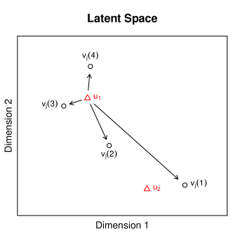
Figure 1: Depiction of the multilogit-bilinear model in latent space. For variable $j$, individual 1 is more likely to choose response 3 or 4 than individual 2 is.

The estimation task is also non-trivial in part also because of the non-convexity of the rank constraint. In addition, overfitting issues due to the so-called separability problems inherent of such models cause some of the parameters wandering off to infinity. Consequently, Groenen and Josse (2016) suggested a majorization approach to estimate the parameters but minimized a penalized deviance using the trace norm. Note that random-effects version of this model (assuming a Gaussian distribution on the latent variables) has been studied in Moustaki and Knott (2000) who also highlighted the necessity to resort to regularization.

3.2 Multiple Correspondence Analysis

MCA has been successfully applied to visualize the relationship between categorical variables on many fields such as social sciences, marketing, health, psychology, educational research, political science, genetics, etc. (Greenacre and Blasius, 2006). MCA is also known as homogeneity analysis or dual scaling (Michailidis and de Leeuw, 1998; Nishisato, 1980; de Leeuw, 2014; le Roux, 2010; Husson et al, 2016b).

To characterize MCA, we begin by defining from the data matrix ${\bf X}$ with $n$ individuals and $m$ variables, the indicator matrix ${\bf A}=\left[{\bf A}^{1}|\cdots|{\bf A}^{m}\right]$ so that ${\bf A}^{j}\in\{0,1\}^{n\times C_{j}}$, with row $i$ corresponding to a dummy coding of $x_{ij}$. Alternatively, with $C=\sum_{j}C_{j}$ the total number of levels across all variables, define the so-called Burt matrix ${\bf B}={\bf A}^{T}{\bf A}\in\mathbb{Z}^{C\times C}$, which contains all two-way tables between pairs of variables. Note that ${\bf B}$ also has a block form, with $B^{j,j^{\prime}}={\bf A}_{j}^{T}{\bf A}_{j^{\prime}}$. For example, with $m=2$ variables with $C_{1}=2$ and $C_{2}=3$ levels respectively, then

$${\bf X}=\begin{pmatrix}1&1\\ 2&3\\ 1&2\\ 2&3\\ 2&2\\ 2&2\end{pmatrix}\;\;\;\Longleftrightarrow\;\;\;{\bf A}=\begin{pmatrix}1&0&&1&0&0\\ 0&1&&0&0&1\\ 1&0&&0&1&0\\ 0&1&&0&0&1\\ 0&1&&0&1&0\\ 0&1&&0&1&0\end{pmatrix}\;\;\;\Longrightarrow\;\;\;{\bf B}=\begin{pmatrix}2&0&&1&1&0\\ 0&4&&0&2&2\\ &&&&&\\ 1&0&&1&0&0\\ 1&2&&0&3&0\\ 0&2&&0&0&2\\ \end{pmatrix}$$

Note that ${\bf X}$ and ${\bf A}$ are equivalent codings of the data, whereas some information is lost in computing ${\bf B}$. Write $p_{j}(c)=\frac{1}{n}A_{\cdot c}^{j}$ for the $c$th normalized column margin of ${\bf A}^{j}$, with ${\bf p}=({\bf p}_{1},\ldots,{\bf p}_{m})^{T}$. All row margins of ${\bf A}$ are exactly $m$, and both the row and column margins of ${\bf B}$ are $mnp$. Then, we can proceed in two nearly-equivalent ways to perform MCA, corresponding operationally to a standard CA on either the indicator matrix ${\bf A}$ or the Burt matrix ${\bf B}$. Forming the pseudo-residual matrices as before (Section 2.2) for each of ${\bf A}$ and ${\bf B}$ and simplifying, we obtain

$${\bf Z}_{\bf A} =\frac{1}{\sqrt{mn}}({\bf A}-{\mathds{1}}{\bf p}^{T}){\bf D}_{\bf p}^{-1/2}$$ (9)

$${\bf Z}_{\bf B} =\frac{1}{mn}{\bf D}_{\bf p}^{-1/2}({\bf B}-n{\bf p}{\bf p}^{T}){\bf D}_{\bf p}^{-1/2}$$

Since ${\bf A}^{T}{\mathds{1}}{\bf p}^{T}={\bf p}{\mathds{1}}^{T}{\mathds{1}}{\bf p}^{T}=n{\bf p}{\bf p}^{T}$, it follows immediately that ${\bf Z}_{\bf B}={\bf Z}_{\bf A}^{T}{\bf Z}_{\bf A}$, so that if ${\bf Z}_{\bf A}$ has SVD ${\bf U}{\bf D}{\bf V}^{T}$, then ${\bf Z}_{\bf B}={\bf V}{\bf D}^{2}{\bf V}^{T}$, and we can recover the MCA coefficients for the Burt-matrix form from the coefficients for the indicator-matrix form (but not vice-versa). We denote $\bm{\widehat{\Gamma}_{\text{MCA}}}$ to be the MCA decomposition ${\bf U}_{K}{\bf D}_{K}{\bf V}_{K}^{T}$ of ${\bf Z}_{\bf A}$.

This specific choice of weighting and transformation in MCA implies that the principal components, denoted $\bf{f}_{k}$ for $k=1,...,K$ satisfy:

$$\bf{f}_{k}=\operatorname*{arg\,max}_{\bf{f}_{k}\in{\mathbb{R}}^{n}}\sum_{j=1}^{m}\eta^{2}(\bf{f}_{k},X_{m})$$

with the constraint that $\bf{f}_{k}$ is orthogonal to $\bf{f}_{k}^{\prime}$ for all $k^{\prime}<k$ and $\eta^{2}$ the square of the correlation ratio (in an analysis of variance sense). This formulation highlights that MCA can be seen as the counterpart of PCA for categorical data. In addition, the distances between the rows coincide with the $\chi^{2}$ distances. MCA analysis mainly consists of interpreting the graphical outputs where rows are represented with ${\bf U}{\bf D}{\bf D}_{\bf p}^{-1/2}$ and categories with ${\bf V}{\bf D}{\bf D}_{\bf p}^{-1/2}$ to identify rows with the same profile of response and association between categories. More properties are given in Husson and Josse (2014).

3.3 MCA as One-Step Likelihood Estimates

Our main results in this section is to show that the low-rank least-squares decompositions of the pseudo-residual matrices ${\bf Z}_{\bf A}$ may be viewed as a one-step estimate for the cognate model discussed in Section 3.1 the multilogit-bilinear.

The rationale of the approach is the following one. Each model represented in Table 1 is parametrized by $(\bm{\beta},\bm{\Gamma})$, with the constraint $\textrm{rank}(\bm{\Gamma})\leq K$. Maximizing $\ell(\bm{\beta},\bm{\Gamma};{\bf X})$ is difficult owing to the non-convex constraint. If instead we Taylor expand $\ell$ around the independence model $(\bm{\beta}_{0},0)$ to obtain $\tilde{\ell}(\bm{\beta},\bm{\Gamma})$, a quadratic function of its arguments, then maximizing the latter amounts to a generalized singular value decomposition, which can be performed efficiently. Moreover, the generalized singular value problem is precisely the one we solve to obtain the row and column coordinates in MCA.

Principal Component Method	Cognate Likelihood Model
CA	Log-bilinear Poisson (3)
Indicator MCA	Multilogit-bilinear Model (8)

Table 1: Relationships between principal component methods for contingency tables and their cognate likelihood methods. Each of the methods in the first row can be characterized as one-step estimates of the models in the second.

Quadratic Functions of a Matrix

Let $\zeta=\binom{\beta}{\text{vec}(\Gamma)}$ denote the real vector of all the model’s parameters with $\zeta_{0}=\binom{\beta_{0}}{0}$, and define the function $\tilde{\ell}$ to be the second-order Taylor approximation:

$$\tilde{\ell}(\beta,\Gamma)=\ell(\zeta_{0})+\ell^{\prime}(\zeta_{0})^{T}(\zeta-\zeta_{0})+\frac{1}{2}(\zeta-\zeta_{0})^{T}\ell^{\prime\prime}(\zeta_{0})(\zeta-\zeta_{0})$$

To begin, we establish a simple technical result that will arise in the proof. For matrices ${\bf G},{\bf H}$ of the same shape, we use the notation $\langle{\bf G},{\bf H}\rangle=\textrm{Tr}({\bf G}^{T}{\bf H})=\sum_{ij}G_{ij}H_{ij}$ to denote the Frobenius inner product.

Lemma 1.

Let ${\bf G}\in\mathbb{R}^{n\times n},{\bf H}_{1}\in\mathbb{R}^{n\times n},{\bf H}_{2}\in\mathbb{R}^{m\times m}$, with ${\bf H}_{1},{\bf H}_{2}\succ 0$. Then the problem

$$\textrm{argmax}_{\bm{\Gamma}:\,\textnormal{rank}(\bm{\Gamma})\leq K}\langle\bm{\Gamma},{\bf G}\rangle-\frac{1}{2}\|{\bf H}_{1}\bm{\Gamma}{\bf H}_{2}\|_{F}^{2}$$ (10)

is solved by

$$\bm{\Gamma}^{*}={\bf H}_{1}^{-1}\left[\textnormal{SVD}_{K}({\bf H}_{1}^{-1}{\bf G}{\bf H}_{2}^{-1})\right]{\bf H}_{2}^{-1}$$

Lemma (1) proven in Appendix 6.1 is easy but vital, since it gives us a target to aim for when we construct Newton approximations to the log-likelihoods of interest. The first-order term in our Taylor expansion is necessarily of the form $\langle\bm{\Gamma},{\bf G}\rangle$, where $G_{ij}$ is simply the gradient with respect to entry $\Gamma_{ij}$. Hence, if we could only show the second derivative term is of the form $-\frac{1}{2}\|{\bf H}_{1}\bm{\Gamma}{\bf H}_{2}\|_{F}^{2}$, then our problem would reduce to a generalized singular value decomposition.

MCA and the Multilogit-Bilinear Model

Theorem 2.

The one-step likelihood estimate for the model (8) with rank constraint $K$, obtained by expanding around the independence model $(\bm{\beta}_{0}=\log\bm{p},\bm{\Gamma}_{0}=0)$, is $(\bm{\beta}_{0},\bm{\widehat{\Gamma}_{\text{MCA}}})$.

The log-likelihood for the model (8) is

$$\ell(\bm{\beta},\bm{\Gamma};{\bf A})=\beta^{j}(a_{ij})+\Gamma_{i}^{j}(a_{ij})-\log\left(\sum_{c=1}^{C_{j}}e^{\beta^{j}(c)+\Gamma_{i}^{j}(c)}\right)$$

It is easy to show (see Appendix 6.2), that that the total contribution in the second-order Taylor approximation evaluating at $(\bm{\beta}_{0},0)$ of the linear term is $\langle\bm{\Gamma},{\bf A}-{\mathds{1}}{\bf p}^{T}\rangle$ and that the total contribution of the second derivatives in $\bm{\Gamma}$ is $-\frac{1}{2}\|\bm{\Gamma}{\bf D}_{p}^{1/2}\|_{F}^{2}$. Thus, using Lemma 1, the solution is given by the rank $K$ SVD of $({\bf A}-{\mathds{1}}{\bf p}^{T}){\bf D}_{\bf p}^{-1/2}$ which is precisely the SVD performed in MCA (equation (9)).

4 Empirical Comparison to MCA

In Section 3.3, we showed that the parameters estimated by MCA can be seen as providing an approximation of the parameters of the multilogit-bilinear model when the interaction is low. We assess empirically Theorem 2 in a simulation study where the data are simulated according to the multilogit-bilinear model varying several parameters:

• the number of individuals $n$ (50, 100, 300), the number of variables $m$ (20, 100, 300). The number of categories per variable is set to 3.

• the number of terms of the interaction $K$ (2, 6)

• the ratio of the first singular value to the second singular value $(d_{1}/d_{2})$ (2, 1). When $K$ is greater than 2, the subsequent singular values are of the same order of magnitude.

• the strength of the interaction (low, strong)

More precisely:

$$\tilde{\bf u}_{i} \sim\mathcal{N}_{K}\left(0,\begin{pmatrix}d_{1}&0\\ 0&d_{K}\end{pmatrix}\right)$$

$$\tilde{\bf v}_{j}(c) \sim\mathcal{N}_{K}\left(0,\begin{pmatrix}d_{1}&0\\ 0&d_{K}\end{pmatrix}\right)$$

$$\theta_{ij}^{c} =-\frac{1}{2}\|\tilde{\bf u}_{i}-\tilde{\bf v}_{j}(c)\|^{2}$$

$$\mathbb{P}(x_{ij}=c) \propto e^{\theta_{ij}^{c}}$$

The strength of the interaction is controlled by multiplying the singular values by a term equal to 0.1 (low) or 1 (strong). To estimate the parameters of the multilogit model (8) we use the majorization algorithm suggested in Groenen and Josse (2016) implemented in the R package mmca (Groenen and Josse, 2015) without any penalty. We perform MCA using the R package FactoMineR (Husson et al, 2016a). A representative extract of the results is given in Table 2. The standard deviations of the MSEs are very small and vary from the order of $10^{-5}$ to $10^{-3}$ (for small sample size). Thus, the MSEs can be directly analyzed to compare the estimators.

	$n$	$p$	rank	ratio	strength	model	MCA
1	50	20	2	1	0.1	0.044	0.035
2	50	20	2	1	1	0.020	0.045
3	50	20	2	2	0.1	0.048	0.036
4	50	20	2	2	1	0.0206	0.042
5	50	20	6	1	0.1	0.111	0.064
6	50	20	6	1	1	0.045	0.026
7	50	20	6	2	0.1	0.115 (0.028)	0.071
8	50	20	6	2	1	0.032	0.051
9	300	100	2	1	0.1	0.005	0.006
10	300	100	2	1	1	0.004	0.042
11	300	100	2	2	0.1	0.0047	0.005
12	300	100	2	2	1	0.0037 (0.00369)	0.040
13	300	300	2	1	0.1	0.003	0.004
14	300	300	2	1	1	0.002	0.039
15	300	300	2	2	0.1	0.003	0.004
16	300	300	2	2	1	0.002	0.039
17	300	100	6	1	0.1	0.019	0.015
18	300	100	6	1	1	0.011	0.023
19	300	100	6	2	0.1	0.018 (0.010)	0.017
20	300	100	6	2	1	0.010	0.056
21	300	300	6	1	0.1	0.011	0.008
22	300	300	6	1	1	0.006	0.022
23	300	300	6	2	0.1	0.009	0.012
24	300	300	6	2	1	0.006	0.061

Table 2: Root mean square error (RMSE) between true probabilities and estimated ones by the multilogit model and MCA. In bold the smallest MSEs; in italic when MCA results are of the same order of magnitude than the ones obtained by the model. For cases, 7, 12 and 19, the error obtained when using a penalized version of the likelihood to estimate the model parameters (Groenen and Josse, 2016) is also given in brackets.

As expected, when the strength of the interaction is low (0.1), both methods agree: the parameters estimated by MCA and by the majorization algorithm are very correlated to the true parameters whatever the scenario and the MSEs are of the same order of magnitude. Thus, MCA is a straightforward alternative, computationally fast and easy to run, to accurately estimate the parameters of the multilogit-bilinear model. When the signal is strong different patterns occur. Figure 2 illustrates a case with a strong first dimension of variability.

Figure 2: Estimation of the parameters by MCA and by the majorization algorithm in a case with a strong interaction and first dimension. The parameters are $n=300,p=100,r=2$.

The majorization algorithm recovers well the true dimensions whereas MCA exhibits an horseshoe effect. Its second dimension can be viewed as an artifact. Consequently, MCA does not seem appropriate to estimate the parameters of multilogit-bilinear model. Nevertheless, one can note that the signal is not completely lost since MCA third dimension of variability corresponds to the true second one. On all the experiments carried out, we also saw situations where both MCA and the majorization algorithm exhibit an horshoe effect (Guttman, 1953). It could be interesting to investigate more the understanding of this behavior in the context of the multilogit model as it was done in Baccini et al (1994), de Leeuw (2007) and Diaconis et al (2008) in the framework of CA and multidimensional scaling. Nevertheless, when the signal is strong even if MCA is less appropriate to estimate the parameters (the MSEs are around 10 times larger), we feel after inspecting many plots, that the approximation is accurate enough and will often lead to the same interpretation of the results. This is in agreement with what was observed in CA by der Heijden et al (1994). Finally, it may seem surprising to see that MCA can provide better estimates than the model ones. This occurs in what can be considered as difficult settings with small $n$ and $p$ and/or noisy data where the strength of the relationship is weak and/or the rank $K$ is large (cases 1, 3, 5, 6, 7). In such situations, the majorization algorithm may encounter difficulties and it is necessary to resort to regularization. If we use a regularized version with the amount of shrinkage determined by cross-validation (Groenen and Josse, 2016), the error for case 7 is then equal to 0.028 instead of 0.115 and improves on MCA. On the contrary, the impact of regularization is less crucial in ”easy” frameworks (case 12). The results are reproducible with the R code provided on a github repository (Josse, 2016).

5 Discussion

Theoretical connections between CA and the log-bilinear model were suggested in the literature but it was lacking for MCA. In this paper, we showed that MCA can be seen as a linearized estimate of the parameters of the multinomial logit bilinear model. Thus, MCA can be used as a proxy to estimate the model’s parameters. In a simulation study, we showed that MCA is particularly well fitted in regimes with small interaction and often provides a good approximation in the other cases. These tight connections allow a better understanding of both models and exploratory methods and going back and forth is part of the process to enhance the comprehension of the approaches and give them a larger scope.

For instance, regularization in the multi-logit model is crucial for better estimation in noisy schemes but the practice is less common in MCA (see Takane and Hwang (2006) and Josse et al (2012) in the framework of missing values). The established relationship between MCA and the multi-logit model greatly encourages to regularize MCA to tackle overfitting issues. In a similar way, graphical outputs are at the core of MCA analysis and almost never used within the probabilistic framework. The experience in the graphical representations in MCA should be used to display the results of the multi-logit model to enhance the interpretation of the results. Finally, we should also mention that MCA is a very powerful way to predict missing values (Audigier et al, 2015), the connection with the model gives more rational and strengthens this good behavior.

We finish by discussing some opportunities for further research. A natural area that should be investigated is to extend mixtures of PCA (Tipping and Bishop, 1999) to categorical data with mixtures of MCA. Since no model was associated to MCA, this mixture model was never considered. Such an approach would allow to get rid of the strong hypothesis of independence between categorical variables within a cluster that is often assumed. Another point that can be considered is the analysis of mixed data (both continuous and categorical data) with the method factorial analysis for mixed data (FAMD) (Escofier, 1979; Kiers, 1991) and data structured in groups of variables with methods such as multiple factor analysis (MFA) (Pagès, 2015). The extension of the theoretical connections between a cognate model and these exploratory methods is not straightforward since specific weightings are applied to balance the influence of variables of different nature. Finally, no method is available to select the rank in MCA and few methods are available to get confidence areas around the results. Using model selections criteria for the multinomial logit bilinear model should at least give hints on the number of relevant dimensions which is crucial for the MCA analysis. This point is definitively a worthwhile enterprise.

6 Appendix: Proofs

6.1 Proof of Lemma 1

Proof.

Change variables to $\widetilde{\Gamma}=H_{1}\Gamma H_{2}$ and complete the square with constant $g=\frac{1}{2}\|H_{1}^{-1}GH_{2}^{-1}\|_{F}^{2}$. Then we obtain

$$\langle\Gamma,G\rangle-\frac{1}{2}\|H_{1}\Gamma H_{2}\|_{F}^{2}-g =\langle H_{1}^{-1}\widetilde{\Gamma}H_{2}^{-1},G\rangle\;-\;\frac{1}{2}\|\widetilde{\Gamma}\|_{F}^{2}\;-\;\frac{1}{2}\|H_{1}^{-1}GH_{2}^{-1}\|_{F}^{2}$$

$$=\langle\widetilde{\Gamma},H_{1}^{-1}GH_{2}^{-1}\rangle\;-\;\frac{1}{2}\|\widetilde{\Gamma}\|_{F}^{2}\;-\;\frac{1}{2}\|H_{1}^{-1}GH_{2}^{-1}\|_{F}^{2}$$

$$=-\frac{1}{2}\|\widetilde{\Gamma}-H_{1}^{-1}GH_{2}^{-1}\|_{F}^{2}$$

Solving for $\widetilde{\Gamma}$ amounts to a rank-$K$ SVD, and we transform back to obtain the result. ∎

6.2 Proof of Theorem 2

Proof.

The log-likelihood for the model (7) is

$$\ell(\bm{\beta},\bm{\Gamma};{\bf A})=\beta^{j}(a_{ij})+\Gamma_{i}^{j}(a_{ij})-\log\left(\sum_{c=1}^{C_{j}}e^{\beta^{j}(c)+\Gamma_{i}^{j}(c)}\right)$$

Differentiating once with respect to $\Gamma_{i}^{j}(c)$, we obtain

$$\frac{\partial\ell}{\partial\Gamma_{i}^{j}(c)}=1_{x_{ij}=c}-\frac{e^{\beta^{j}(c)+\Gamma_{i}^{j}(c)}}{\sum_{c^{\prime}=1}^{C_{j}}e^{\beta^{j}(c^{\prime})+\Gamma_{i}^{j}(c^{\prime})}}$$ (11)

Evaluating (11) at $(\beta_{0},0)$ gives

$$A_{i}^{j}(c)-p^{j}(c),$$ (12)

so that the total contribution of the linear term is $\langle\Gamma,A-1p^{T}\rangle$.

Differentiating (11) with respect to $\beta^{j^{\prime}}(c^{\prime})$, and evaluating at $(\beta_{0},0)$ gives

$$\frac{\partial\ell}{\partial\Gamma_{i}^{j}(c)\partial\beta^{j^{\prime}}(c^{\prime})}=\left\{\begin{matrix}p^{j}(c)p^{j}(c^{\prime})-p^{j}(c)1_{c=c^{\prime}}&j=j^{\prime}\\ 0&\text{ o.w. }\\ \end{matrix}\right.$$

Thus, the total contribution to $\tilde{\ell}$ of crossed partials involving $\beta^{j}(c^{\prime})$ is

$$\frac{1}{2}(\beta^{j}(c)-\beta_{0}^{j}(c))\sum_{i,c^{\prime}}\frac{\partial\ell}{\partial\Gamma_{i}^{j}(c^{\prime})\partial\beta^{j}(c^{\prime})}\Gamma_{i}^{j}(c^{\prime}) =\frac{1}{2}(\beta^{j}(c)-\beta_{0}^{j}(c))p^{j}(c)\sum_{i,c^{\prime}}\Gamma_{i}^{j}(c^{\prime})(p^{j}(c^{\prime})-1_{c=c^{\prime}})$$

$$=\frac{1}{2}(\beta^{j}(c)-\beta_{0}^{j}(c))p^{j}(c)\sum_{i}-\Gamma_{i}^{j}(c)$$

Differentiating (11) with respect to $\Gamma_{i^{\prime}}^{j^{\prime}}(c^{\prime})$ and evaluating at $(\beta_{0},0)$ gives

$$\frac{\partial\ell}{\partial\Gamma_{i}^{j}(c)\partial\Gamma_{i^{\prime}}^{j^{\prime}}(c^{\prime})}=\left\{\begin{matrix}p^{j}(c)p^{j}(c^{\prime})-p^{j}(c)1_{c=c^{\prime}}&j=j^{\prime},i=i^{\prime}\\ 0&\text{ o.w. }\\ \end{matrix}\right.$$

The total contribution of the second derivatives in $\Gamma$ is then

$$-\frac{1}{2}\sum_{i,j,c}\Gamma_{i}^{j}(c)^{2}p^{j}(c)+\frac{1}{2}\sum_{i,j,c,c^{\prime}}p^{j}(c)\Gamma_{i}^{j}(c)p^{j}(c^{\prime})\Gamma_{i}^{j}(c^{\prime}) =-\frac{1}{2}\|\Gamma D_{p}^{1/2}\|_{F}^{2}+\frac{1}{2}\sum_{i,j}\left(\sum_{c}\Gamma_{i}^{j}(c)p^{j}(c)\right)^{2}$$

$$=-\frac{1}{2}\|\Gamma D_{p}^{1/2}\|_{F}^{2}$$

Overall, then, we have

$$\tilde{\ell}(\beta,\Gamma)=\langle\Gamma,A-1p^{T}\rangle-\frac{1}{2}\|\Gamma D_{p}^{1/2}\|_{F}^{2}-\frac{1}{2}1^{T}\Gamma D_{p}(\beta-\beta_{0})$$

∎

Acknowledgment

We thank Antoine de Falguerolles for interesting discussions and his ”glim” view on exploratory methods.

References

- Agresti (2013) Agresti A (2013) Categorical Data Analysis, 3rd Edition. Wiley
- Allen et al (2014) Allen GI, Grosenick L, Taylor J (2014) A generalized least-square matrix decomposition. Journal of the American Statistical Association 109(505):145–159
- Audigier et al (2015) Audigier V, Husson F, Josse J (2015) Mimca: Multiple imputation for categorical variables with multiple correspondence analysis. Statistics and Computing
- Baccini et al (1994) Baccini A, Caussinus H, de Falgurolles A (1994) Diabolic horseshoes. In: Proceedings of the international workshop on Statistical modeling
- Benzécri (1973) Benzécri JP (1973) L’analyse des données. Tome II: L’analyse des correspondances. Dunod
- Buntine (2002) Buntine W (2002) Variational extensions to EM and multinomial PCA. In: Elomaa T, Mannila H, Toivonen H (eds) Machine Learning: ECML 2002, Lecture Notes in Computer Science, vol 2430, Springer Berlin Heidelberg, pp 23–34
- Caussinus (1986) Caussinus H (1986) Models and uses of principal component analysis (with discussion). In: de Leeuw J, Heiser W, Meulman J, Critchley F (eds) Multidimensional Data Analysis, DSWO Press, pp 149–178
- Choulakian (1996) Choulakian V (1996) Generalized bilinear models. Psychometrika 61 (2):271–283
- Christensen (2010) Christensen R (2010) Log-Linear Models. Springer-Verlag, New York
- Collins et al (2001) Collins M, Dasgupta S, Schapire RE (2001) A generalization of principal component analysis to the exponential family. In: Advances in Neural Information Processing Systems, MIT Press
- de Falguerolles (1998) de Falguerolles A (1998) Log-bilinear biplot in action. In: Blasius J, Greenacre M (eds) Visualisation of categorical data, Academic Press, pp 527–533
- De Leeuw (2006) De Leeuw J (2006) Principal component analysis of binary data by iterated singular value decomposition. Computational Statistics and Data Analysis 50(1):21–39
- de Leeuw et al (1985) de Leeuw J, Mooijaart A, van der Leeden R (1985) Fixed factor score models with linear restrictions. Tech. rep., Leiden: Department of Data theory
- Denis and Gower (1994) Denis JB, Gower JC (1994) Asymptotic covariances for the parameters of biadditive models. Utilitas Mathematica 46:193–205
- Denis and Gower (1996) Denis JB, Gower JC (1996) Asymptotic confidence regions for biadditive models: interpreting genotype-environment interactions. Applied Statistics 45(4):479–493
- Diaconis et al (2008) Diaconis P, Goel S, Holmes S (2008) Horseshoes in multidimensional scaling and local kernel methods. Annals of Applied Statistics 2(3):777–807
- van Eeuwijk (1995) van Eeuwijk FA (1995) Multiplicative interaction in generalized linear models. Biometrics 51(3):1017–1032
- Escofier (1979) Escofier B (1979) Traitement simultané de variables quantitatives et qualitatives en analyse factorielle. Les cahiers de l’analyse des données 4(2):137–146
- Escoufier (1982) Escoufier Y (1982) The analysis of simple and multiple contingency tables. In: Proceedings of the international meeting of the analysis of multidimensional contingency tables, R. Coppi, Rome, Italy, pp 53–77
- Gabriel (1978) Gabriel KR (1978) Least squares approximation of matrices by additive and multiplicative models. Journal of the Royal Statistical Society Series B 40 (2):186–196
- Gabriel (1998) Gabriel KR (1998) Generalised bilinear regression. Biometrika 85 (2):689–700
- Gauch (1988) Gauch H (1988) Model selection and validation for yield trials with interaction. Biometrics 44:705–715
- Goodman (1985) Goodman LA (1985) The analysis of cross-classified data having ordered and/or unordered categories: Association models, correlation models, and asymmetry models for contingency tables with or without missing entries. Annals of Statistics 13:10–69
- Gower et al (2011) Gower J, Lubbe S, le Roux N (2011) Understanding Biplots. John Wiley & Sons
- Gower and Hand (1995) Gower JC, Hand DJ (1995) Biplots. Chapman and Hall/CRC
- Greenacre (1984) Greenacre M (1984) Theory and Applications of Correspondence Analysis. Acadamic Press
- Greenacre and Blasius (2006) Greenacre M, Blasius J (2006) Multiple Correspondence Analysis and Related Methods. Chapman & Hall/CRC
- Greenacre (2007) Greenacre MJ (2007) Correspondence Analysis in Practice, Second Edition. Chapman & Hall
- Groenen and Josse (2016) Groenen P, Josse J (2016) Multinomial mca. arXiv:160303174
- Groenen and Koning (2006) Groenen P, Koning A (2006) A new model for visualizing interactions in analysis of variance. In: Greenacre MJ, Blasius J (eds) Multiple correspondence analysis and related methods, Chapman & Hall, pp 487–502
- Groenen and Josse (2015) Groenen PJ, Josse J (2015) mmca: Multinomial Multiple Correspondence Analysis. R package version 0.1
- Guttman (1953) Guttman L (1953) A note on sir cyril burt’s factorial analysis of qualitative data. Psychological MethodBritish Journal of Statistical Psychology 6:21–40
- Van der Heijden et al (1989) Van der Heijden PGM, De Falguerolles A, De Leeuw J (1989) A combined to contingency table analysis using correspondence analysis and loglinear analysis. Applied Statistics 38:249–292
- der Heijden and de Leeuw (1985) der Heijden PGMV, de Leeuw J (1985) Correspondence analysis used complementary to loglinear analysis. Psychometrica 50:429–447
- der Heijden et al (1994) der Heijden PGMV, Mooijaart A, Takane Y (1994) Correspondence analysis and contingency table models. In: Greenacre M, Blasius J (eds) Correspondence analysis in the social sciences. Recent developments and applications, London: Academic Press., pp 79–111
- Hoff (2009) Hoff P (2009) Multiplicative latent factor models for description and prediction of social networks. Computational & Mathematical Organization Theory 15(4):261–272
- Husson and Josse (2014) Husson F, Josse J (2014) Multiple correspondence analysis. In: Visualization and Verbalization of Data, CRC Press, Taylor & Francis, pp 165–184
- Husson et al (2010) Husson F, Lê S, Pagès J (2010) Exploratory Multivariate Analysis by Example Using R. Chapman & Hall/CRC
- Husson et al (2016a) Husson F, Josse J, Le S, Mazet J (2016a) FactoMineR: Multivariate Exploratory Data Analysis and Data Mining. R package version 1.32
- Husson et al (2016b) Husson F, Josse J, Saporta G (2016b) Jan de leeuw and the french school of data analysis. Journal of Statistical Software
- Josse (2016) Josse J (2016) Github repository. URL https://github.com/julierennes
- Josse et al (2012) Josse J, Chavent M, Liquet B, Husson F (2012) Handling missing values with regularized iterative multiple correspondence analysis. Journal of classification 29(1):91–116
- Kiers (1991) Kiers HAL (1991) Simple structure in component analysis techniques for mixtures of qualitative and quantitative variables. Psychometrika 56:197–212
- Lazarsfeld and Henry (1968) Lazarsfeld PF, Henry NW (1968) Latent structure analysis. Boston: Houghton Mifflin
- Lebart et al (1998) Lebart L, Salem A, Berry L (1998) Exploring Textual Data. Springer Science & Business Media
- de Leeuw (2007) de Leeuw J (2007) A horseshoe for multidimensional scaling. Tech. rep.
- de Leeuw (2014) de Leeuw J (2014) History of non linear principal component analysis. In: Blasius J, Greenacre MJ (eds) Visualization and Verbalization of Data, Chapman & Hall
- Li and Tao (2013) Li J, Tao D (2013) Simple exponential family pca. Neural Networks and Learning Systems, IEEE Transactions on 24(3):485–497
- van der Linden and Hambleton (1997) van der Linden W, Hambleton R (1997) Handbook of Modern Item Response Theory. Springer-Verlag, New York
- Mandel (1969) Mandel J (1969) The partitioning of interaction in analysis of variance. Journal of the research of the national bureau of standards, Series B 73:309–328
- Michailidis and de Leeuw (1998) Michailidis G, de Leeuw J (1998) The gifi system of descriptive multivariate analysis. Statistical Science 13:307–336
- Moustaki and Knott (2000) Moustaki I, Knott M (2000) Generalized latent trait models. Psychometrika 65(3):391–411
- Nelder and Wedderburn (1972) Nelder J, Wedderburn RWM (1972) Generalized linear models. Journal of the Royal Statistical Society Series A (General) 135(3):370–384
- Ng et al (2002) Ng AY, Jordan MI, Weiss Y, et al (2002) On spectral clustering: Analysis and an algorithm. Advances in neural information processing systems 2:849–856
- Nishisato (1980) Nishisato S (1980) Analysis of Categorical Data: Dual Scaling and its Applications. University of Toronto Press, Toronto
- Pagès (2015) Pagès J (2015) Multiple Factor Analysis with R. Chapman & Hall/CRC
- Raftery et al (2011) Raftery A, Niu X, Hoff P, Yeung K (2011) Fast inference for the latent space network model using a case-control approximate likelihood. Journal of Computational and Graphical Statistics
- Rooij and Heiser (2005) Rooij M, Heiser W (2005) Graphical representations and odds ratios in a distance-association model for the analysis of cross-classified data. Psychometrika 70(1):99–122
- Rooij (2008) Rooij Md (2008) The analysis of change, newton’s law of gravity and association models. Journal of the Royal Statistical Society: Series A (Statistics in Society) 171(1):137–157
- le Roux (2010) le Roux B (2010) Multiple Correspondence Analysis. SAGE publications, CA: Thousand Oaks
- Salmon et al (2014) Salmon J, Harmany Z, Deledalle C, Willett R (2014) Poisson noise reduction with non-local pca. Journal of Mathematical Imaging and Vision 48(2):279–294
- Shi and Malik (2000) Shi J, Malik J (2000) Normalized cuts and image segmentation. Pattern Analysis and Machine Intelligence, IEEE Transactions on 22(8):888–905
- Takane and Hwang (2006) Takane Y, Hwang H (2006) Regularized multiple correspondence analysis. In: Blasius J, Greenacre MJ (eds) Multiple Correspondence Analysis and Related Methods, Chapman & Hall, pp 259–279
- Tipping and Bishop (1999) Tipping ME, Bishop CM (1999) Mixtures of probabilistic principal component analyzers. Neural Comput 11(2):443–482
- Turner and Firth (2015) Turner H, Firth D (2015) Generalized nonlinear models in R: An overview of the gnm package. R package version 1.0-8
- Vicente-Villardon et al (2006) Vicente-Villardon J, Galindo-Villardon M, Blazquez-Zaballos A (2006) Logistic biplots. in: Multiple correspondence analysis and related methods. In: Greenacre MJ, Blasius J (eds) Multiple correspondence analysis and related methods, London, Chapman & Hall., pp 503–522