Wave equation for generalized Zener model containing complex order fractional derivatives

Abstract

We study waves in a viscoelastic rod whose constitutive equation is of generalized Zener type that contains fractional derivatives of complex order. The restrictions following from the Second Law of Thermodynamics are derived. The initial-boundary value problem for such materials is formulated and solution is presented in the form of convolution. Two specific examples are analyzed.

Mathematics Subject Classification (2010): Primary: 26A33; Secondary: 74D05 Keywords: Fractional derivative of complex order, constitutive equation, thermodynamical restriction, wave propagation

1 Introduction

Fractional calculus is intensively used for the modelling of various problems arising in mechanics, physics, engineering, medicine, economy, biology, chemistry, etc; see [22, 23] and references therein as well as our recent books [8, 9]. Especially, in viscoelasticity, differential operators of arbitrary real order were successfully applied, since fractional derivatives, being nonlocal operators, describe intrinsic properties of a material with a ”memory”, cf. [18]. Derivatives of purely imaginary order were initially studied in [17], and later, those of complex order were used to describe viscoelastic properties, were studied in [19, 20, 21]. However, in these papers the authors did not consider restrictions for constitutive equations that follow from the Second Law of Thermodynamics. The waves in viscoelastic media have been studied in many papers. We mention few recent studies: In [14], wave propagation in viscoelastic bodies, in [13], nonlinear fractional viscoelastic constitutive equations, while in [24] the waves have been studied both analytically and experimentally. The first fractional generalization of the Zener model for a viscoelastic body was considered in [2] while the distrubuted-order fractional derivatives were considered in [6, 7]. Rheological models with fractional damping elements and thermodynamical restrictions were studied in [16] and those with thermal and viscoelastic relaxation effects and diffusion phenomena were studied in [12]. We note that a generalized wave equation, with fractional derivatives, for a viscoelastic material given in [25], is a special case of our model in this paper.

To the best of our knowledge, so far only factional derivatives of real order have been used for describing waves in viscoelastic media. In this work, following our previous results [3, 5], we study waves in a viscoelastic rod whose material is described by fractional derivatives of complex order. Our particular interest is related to waves in a specific viscoelastic material described by a generalized Zener standard model. A viscoelastic rod model is given by a system of equations that corresponds to its isothermal motion:

$$\frac{\partial}{\partial x}\sigma(x,t)=\rho\,\frac{\partial^{2}}{\partial t^{2}}u(x,t),$$

$$\sigma(x,t)+a_{1}\,{}_{0}D_{t}^{\alpha}\sigma(x,t)+b_{1}\,{}_{0}\bar{D}_{t}^{\alpha,\beta}\sigma(x,t)=E\,\Big{(}\varepsilon(x,t)+a_{2}\,{}_{0}D_{t}^{\alpha}\varepsilon(x,t)+b_{2}\,{}_{0}\bar{D}_{t}^{\alpha,\beta}\varepsilon(x,t)\Big{)},$$ (1)

$$\varepsilon(x,t)=\frac{\partial}{\partial x}u(x,t),\qquad x\in(0,l],\;\mbox{ or }x\in(0,\infty)\,\,t>0,$$

$0<\alpha<1,\beta>0,$ together with the initial conditions

$$u(x,0)=0,\,\,\,\frac{\partial}{\partial t}u(x,0)=0,\,\,\,\sigma(x,0)=0,\,\,\,\varepsilon(x,0)=0,$$ (2)

and boundary conditions

$$u(0,t)=U(t),\,\,\,u(l,t)=0,$$ (3)

in the case of finite $l$. In the case $l=\infty$ condition (3)₂ is replaced with

$$\lim_{x\to\infty}u(x,t)=0.$$ (4)

Here $u,\sigma$ and $\varepsilon$ are displacement, stress and strain, respectively. Also, $x$ denotes the spatial coordinate oriented along the axis of the rod and $t$ denotes the time.

All our calculations are performed on the time variable and $x$ appears as a parameter. We assume throughout the paper that all the soltions $u$ depending on $x$ and $t$

$$\mbox{are continuous with respect to }x\in[0,l]\mbox{ or }x\in[0,\infty),\mbox{ for almost all }t>0.$$

In the case when $u(x,\cdot)$ is a tempered distribution supported by $[0,\infty),$ then we assume tnat $[0,l]\ni x\mapsto\langle u(x,t),\phi(t)\rangle,$ is continuous for any rapidly decreasing test function $\phi$ ($\phi\in\mathcal{S}(\mathbb{R}^{d})$).

The lenth of the rod is denoted by $l$; in case (4), it is assumed that $l=\infty$. In the sequel, $[0,l]$ (or $(0,l]$), denotes both cases: with $l<\infty$ and $l=\infty.$

Constants $\rho,E,a_{1},a_{2},b_{1},b_{2}\in\mathbb{R}_{+}$ characterize the material. We note that $E$ represents the modulus of elasticity and $\rho$ density of the material. The term ${}_{0}D_{t}^{\alpha}$ is the left Riemann-Liouville fractional derivative operator of order $\alpha$ defined as

$${}_{0}D_{t}^{\alpha}u(x,t)=\frac{1}{\Gamma(1-\alpha)}\frac{d}{dt}\int_{0}^{t}\frac{u(x,\tau)}{(t-\tau)^{\alpha}}d\tau=\frac{d}{dt}\frac{\tau_{+}^{-\alpha}}{\Gamma(1-\alpha)}\ast u(x,\tau)(t),\quad t>0,\,\,\,0<\alpha<1,$$

where we have assumed that $u(x,\cdot)$ is a polynomially bounded locally integrable function supported on $[0,\infty)$, for every $x\geq 0$, and $\ast$ denotes convolution with respect to $t$, $(f\ast g)(t)=\int_{0}^{t}f(t-\tau)g(\tau)\,d\tau$, $t>0$.

Also in (1) we use the following fractional operator of complex order

$${}_{0}\bar{D}_{t}^{\alpha,\beta}:=\frac{1}{2}\Big{(}\hat{b}_{1}\,{}_{0}D_{t}^{\alpha+i\beta}+\hat{b}_{2}\,{}_{0}D_{t}^{\alpha-i\beta}\Big{)},$$

where the dimensions of constants are chosen to be $\hat{b}_{1}=T^{i\beta}$, $\hat{b}_{2}=T^{-i\beta}$, so that $|\hat{b}_{1}|=|\hat{b}_{2}|$ ($T$ is a constant having the dimension of time). This form of a symmetrized fractional derivative of complex order was introduced in [3, 5]. Recall that the form of ${}_{0}\bar{D}_{t}^{\alpha,\beta}$ is adapted to the presumption: a fractional derivative of complex order applied to a real-valued function has to be again real-valued. A dimensionless form is

$${}_{0}\bar{D}_{t}^{\alpha,\beta}u(x,t)=\frac{1}{2}\frac{d}{dt}\bigg{(}\frac{\tau_{+}^{-\alpha+i\beta}+\tau_{+}^{-\alpha-i\beta}}{\Gamma(1-\alpha)}\bigg{)}\ast u(x,\tau)(t),\quad t>0,\,0<\alpha<1,\,\beta>0.$$

The first equation in (1) is the equation of motion with $\rho$ being the density of the material. The second one in (1) is the constitutive equation and coefficients $a_{1},a_{2},b_{1},b_{2}$ satisfy restrictions that will be determined in the next section. Those restrictions follow from the Second Law of Thermodynamics. Recall that in the case of the classical wave equation $u_{tt}=c\,u_{xx}$, for the wave propagation in an elastic media, the corresponding constitutive equation is given by the Hooke law $\sigma=E\,\varepsilon$. The last equation in (1) is the strain measure for small local deformations.

Initial conditions (2) show that there is no initial displacement, velocity, stress and strain, while boundary conditions (3) prescribe displacement at the point $x=0$ and at $x=l$ or infinity.

We introduce dimensionless parameters by a similar consideration as in [4, 15]. Let

$$\bar{x}=\frac{x}{L},\quad\bar{t}=\frac{t}{T},\quad\bar{u}=\frac{u}{L},\quad\bar{\sigma}=\frac{\sigma}{E},\quad\bar{a}_{i}=\frac{a_{i}}{T^{\alpha}},\quad\bar{b}_{i}=\frac{b_{i}}{T^{\alpha}}\,\,\,(i=1,2),\quad\bar{U}=\frac{U}{L},$$

where $T=(a_{2})^{1/\alpha},\ L=(a_{2})^{1/\alpha}\sqrt{\frac{E}{\rho}}$. Note that $\varepsilon$ is already a dimensionless quantity. By inserting dimensionless quantities (and dropping the bar sign) into (1), we obtain

$$\frac{\partial}{\partial x}\sigma(x,t)=\frac{\partial^{2}}{\partial t^{2}}u(x,t),$$

$$\sigma(x,t)+a_{1}\,{}_{0}D_{t}^{\alpha}\sigma(x,t)+b_{1}\,{}_{0}\bar{D}_{t}^{\alpha,\beta}\sigma(x,t)=\varepsilon(x,t)+a_{2}\,{}_{0}D_{t}^{\alpha}\varepsilon(x,t)+b_{2}\,{}_{0}\bar{D}_{t}^{\alpha,\beta}\varepsilon(x,t),$$ (5)

$$\varepsilon(x,t)=\frac{\partial}{\partial x}u(x,t),\qquad x\in(0,l],\,\,\,t>0.$$

Assuming that $\sigma(x,\cdot)$ and $\varepsilon(x,\cdot),x\in[0,l)$ are tempered distributions supported by $[0,\infty),$ and applying the Laplace transform with respect to $t$, ${\cal L}[\sigma(x,t)](x,s)=\tilde{\sigma}(x,s)=\int_{0}^{\infty}e^{-ts}\sigma(x,t)\,dt$, $\mathop{\rm Re}\nolimits s>0$, (and the same for $\varepsilon$), to the constitutive equation (1)₂ we obtain

$$\Big{(}1+a_{1}\,s^{\alpha}+b_{1}\,\big{(}s^{\alpha+i\beta}+s^{\alpha-i\beta}\big{)}\Big{)}\tilde{\sigma}(x,s)=\Big{(}1+a_{2}\,s^{\alpha}+b_{2}\,\big{(}s^{\alpha+i\beta}+s^{\alpha-i\beta}\big{)}\Big{)}\tilde{\varepsilon}(x,s),$$ (6)

from which we express the stress $\sigma(x,t)$ (after applying the inverse Laplace transform) as

$$\sigma(x,t)=\bigg{(}{\cal L}^{-1}\bigg{[}\frac{1+a_{2}\,s^{\alpha}+b_{2}\,(s^{\alpha+i\beta}+s^{\alpha-i\beta})}{1+a_{1}\,s^{\alpha}+b_{1}\,(s^{\alpha+i\beta}+s^{\alpha-i\beta})}\bigg{]}\ast_{t}\varepsilon\bigg{)}(x,t),\quad x\in[0,l],\,\,\,t>0.$$

In the end, this formal calculus will obtain the complete mathematical justification. We use the distributional Laplace transform. Recall that it is defined for locally integrable functions of polynomial growth, and more generally, for tempered distributions supported on $[0,\infty)$. Important examples are ${\cal L}[\delta(t)](s)=1$ and ${\cal L}[H(t)t^{\alpha}/\Gamma(1+\alpha)](s)=1/s^{\alpha+1}$, $\mathop{\rm Re}\nolimits s>0$. The left hand side has extension for $\mathop{\rm Re}\nolimits s=0$ and $|\mathop{\rm Im}\nolimits s|\geq\eta_{0}$, for any $\eta_{0}>0$.

If we now replace $\varepsilon$ from (5)₃ into (5)₂, and then insert the result into (5)₁ we obtain

$$\frac{\partial^{2}}{\partial t^{2}}u(x,t)=L(t)\ast_{t}\frac{\partial^{2}}{\partial x^{2}}u(x,t),\qquad x\in[0,l],\,\,\,t>0,$$ (7)

and the initial and boundary conditions

$$u(x,0)=0,\quad\frac{\partial}{\partial t}u(x,0)=0,\qquad x\in[0,l],$$

$$u(0,t)=U(t),\quad u(l,t)=0\quad(\mbox{or }\,\lim_{x\to\infty}u(x,t)=0),\qquad t>0,$$ (8)

where

$$L(t)={\cal L}^{-1}\bigg{[}\frac{1+a_{2}\,s^{\alpha}+b_{2}\,(s^{\alpha+i\beta}+s^{\alpha-i\beta})}{1+a_{1}\,s^{\alpha}+b_{1}\,(s^{\alpha+i\beta}+s^{\alpha-i\beta})}\bigg{]}(t),\qquad t>0,\,\alpha\in(0,1),\,\beta>0.$$ (9)

In the sequel we shall analyze problem (7)-(8).

Note that it includes several wave equations analyzed earlier. For instance, if the rod is elastic we have $a_{1}=b_{1}=a_{2}=b_{2}=0$, so that $L(t)=\delta(t)$, and we obtain the classical wave equation $\frac{\partial^{2}}{\partial t^{2}}u(x,t)=\frac{\partial^{2}}{\partial x^{2}}u(x,t)$. If the rod is described by a fractional Zener model with derivatives of real order we have $b_{1}=b_{2}=0$ so that $L(t)={\cal L}^{-1}\Big{[}\frac{1+a_{2}\,s^{\alpha}}{1+a_{1}\,s^{\alpha}}\Big{]}(t)$, and problem (7)-(8) reduces to the one treated in [15] with $l=\infty$.

Restrictions on parameters $a_{1},a_{2},b_{1},b_{2},\alpha,\beta$ will be determined in the following Section, in such a way that the physical meaning of the problem remains preserved. In this sense, Remark 2.3 is important.

Remark 1.1

Although it is not obvious, the function $L$ given by (9) is a real valued function of real variable $t>0$. To see this, we recall the theorem of Doetsch [11, p. 293, Satz 2]: A function $L$ is real-valued (almost everywhere) if its Laplace transform is real-valued for all real s in the half-plane of convergence on the right from some real $x_{0}$. Function $\frac{1+a_{2}\,s^{\alpha}+b_{2}\,(s^{\alpha+i\beta}+s^{\alpha-i\beta})}{1+a_{1}\,s^{\alpha}+b_{1}\,(s^{\alpha+i\beta}+s^{\alpha-i\beta})}$ clearly satisfies this condition for $s=x>x_{0}=0$ (cf. [5]).

The paper is organized as follows: Following the procedure proposed by Bagley and Torvik (see [10, 4, 1]), in the next Section 2, we derive thermodynamical restrictions on parameters in (5)₂ in order to preserve the Second Law of Thermodynamics. Then in Section 3 we further examine properties of the Laplace transform of the constitutive equation, which will be needed for the solvability of (7)-(8). The existence and uniqueness of a solution to the wave equation (7) is studied in Section 4, where we also explicitly calculate the solution. Thermodynamical restrictions again come as essential ones with an appropriate sharpness of one of restrictions. Results obtained using analytical tools are numerically illustrated in Section 5.

2 Thermodynamical restrictions

Consider the constitutive equation (5)₂ for $t>0$, $x\in\mathbb{R}_{+}$, $\alpha\in(0,1)$ and $\beta>0$. In the analysis that follows the $x$ variable is omitted; (5)₂ is written in the form

$$\sigma(t)+a_{1}\,{}_{0}D_{t}^{\alpha}\sigma(t)+b_{1}\,{}_{0}\bar{D}_{t}^{\alpha,\beta}\sigma(t)=\varepsilon(t)+a_{2}\,{}_{0}D_{t}^{\alpha}\varepsilon(t)+b_{2}\,{}_{0}\bar{D}_{t}^{\alpha,\beta}\varepsilon(t).$$ (10)

We assume that $\sigma(x,\cdot)$ and $\varepsilon(x,\cdot)$ are polynomially bounded locally integrable functions supported on $[0,\infty)$, for every $x\geq 0$. For the coefficients we assume

$$a_{i},b_{i}\geq 0,\,\,\,i=1,2,\quad\mbox{ and }\quad a_{2}>a_{1}.$$

Thermodynamical restrictions, i.e., the dissipativity condition - the Second Law of Thermodynamics under isothermal conditions - are closely connected with the following additional assumptions:

$$a_{2}b_{1}-a_{1}b_{2}=0,$$ (11)

$$a_{1} \geq 2b_{1}\cosh\frac{\beta\pi}{2}\sqrt{1+\Big{(}\mathop{\rm ctg}\nolimits\frac{\alpha\pi}{2}\mathop{\rm tgh}\nolimits\frac{\beta\pi}{2}\Big{)}^{2}},$$

$$a_{2} \geq 2b_{2}\cosh\frac{\beta\pi}{2}\sqrt{1+\Big{(}\mathop{\rm ctg}\nolimits\frac{\alpha\pi}{2}\mathop{\rm tgh}\nolimits\frac{\beta\pi}{2}\Big{)}^{2}},$$ (12)

$$a_{1} \geq 2b_{1}\cosh\frac{\beta\pi}{2}\sqrt{1+\Big{(}\mathop{\rm tg}\nolimits\frac{\alpha\pi}{2}\mathop{\rm tgh}\nolimits\frac{\beta\pi}{2}\Big{)}^{2}},$$

$$a_{2} \geq 2b_{2}\cosh\frac{\beta\pi}{2}\sqrt{1+\Big{(}\mathop{\rm tg}\nolimits\frac{\alpha\pi}{2}\mathop{\rm tgh}\nolimits\frac{\beta\pi}{2}\Big{)}^{2}},$$ (13)

that will be explained in this section. We will need a strong inequality in (12) for the existence result in Section 3, which will be denoted by (12)_s.

Thermodynamical restrictions will be determined by following the method proposed in [10].

We use the Fourier transform

$${\cal F}[\varphi(x)](\xi)=\hat{\varphi}(\xi)=\int_{\mathbb{R}}e^{-i\xi x}\varphi(x)dx,\;\xi\in\mathbb{R}\;\mbox{ if }\;\varphi\in L^{1}(\mathbb{R}),$$

or in the sense of tempered distributions if $\varphi$ is locally integrable, supported by $[0,\infty)$ and bounded by a polynomial. Applying the Fourier transform to (10) in the sense of distributions (assuming that $\sigma$ and $\varepsilon$ are Fourier transformable), we obtain $\hat{\sigma}(\omega)=\hat{E}(\omega)\hat{\varepsilon}(\omega)$, so that the complex modulus of elasticity is

$$\hat{E}(\omega) =\frac{\hat{P}(\omega)}{\hat{Q}(\omega)}=\frac{\mathop{\rm Re}\nolimits\hat{P}(\omega)+i\mathop{\rm Im}\nolimits\hat{P}(\omega)}{\mathop{\rm Re}\nolimits\hat{Q}(\omega)+i\mathop{\rm Im}\nolimits\hat{Q}(\omega)}$$

$$=\frac{\mathop{\rm Re}\nolimits\hat{P}(\omega)\mathop{\rm Re}\nolimits\hat{Q}(\omega)+\mathop{\rm Im}\nolimits\hat{P}(\omega)\mathop{\rm Im}\nolimits\hat{Q}(\omega)}{\mathop{\rm Re}\nolimits\hat{Q}(\omega)^{2}+\mathop{\rm Im}\nolimits\hat{Q}(\omega)^{2}}+i\frac{\mathop{\rm Im}\nolimits\hat{P}(\omega)\mathop{\rm Re}\nolimits\hat{Q}(\omega)-\mathop{\rm Re}\nolimits\hat{P}(\omega)\mathop{\rm Im}\nolimits\hat{Q}(\omega)}{\mathop{\rm Re}\nolimits\hat{Q}(\omega)^{2}+\mathop{\rm Im}\nolimits\hat{Q}(\omega)^{2}}$$

$$=\mathop{\rm Re}\nolimits\hat{E}(\omega)+i\mathop{\rm Im}\nolimits\hat{E}(\omega),\qquad\omega\in(0,\infty),$$

where $\mathop{\rm Re}\nolimits\hat{E}(\omega)$ and $\mathop{\rm Im}\nolimits\hat{E}(\omega)$ are the loss and the storage modulus. Also,

$$\hat{P}(\omega)=1+a_{2}\,(i\omega)^{\alpha}+b_{2}\,\omega^{\alpha}\Big{(}e^{-\frac{\beta\pi}{2}}e^{i(\frac{\alpha\pi}{2}+\ln\omega^{\beta})}+e^{\frac{\beta\pi}{2}}e^{i(\frac{\alpha\pi}{2}-\ln\omega^{\beta})}\Big{)},\quad\omega>0,$$

$$\hat{Q}(\omega)=1+a_{1}\,(i\omega)^{\alpha}+b_{1}\,\omega^{\alpha}\Big{(}e^{-\frac{\beta\pi}{2}}e^{i(\frac{\alpha\pi}{2}+\ln\omega^{\beta})}+e^{\frac{\beta\pi}{2}}e^{i(\frac{\alpha\pi}{2}-\ln\omega^{\beta})}\Big{)},\quad\omega>0.$$

With $\hat{P}(0)=\hat{Q}(0)=1,$ $\hat{P}$ and $\hat{Q}$ are continuous function for $\omega\in[0,\infty).$ Let

$$f(\tau,\varphi) := \cos\tau\cos(\alpha\varphi)\cosh(\beta\varphi)+\sin\tau\sin(\alpha\varphi)\sinh(\beta\varphi),\qquad\tau\in\mathbb{R},$$ (14)

$$g(\tau,\varphi) := \cos\tau\sin(\alpha\varphi)\cosh(\beta\varphi)-\sin\tau\cos(\alpha\varphi)\sinh(\beta\varphi),\qquad\tau\in\mathbb{R}.$$ (15)

Properties of functions $f$ and $g$ for $\varphi=\pi/2$ were investigated in [5]. It was shown that the extremal values of $f$ and $g$ are attained at points $\tau_{f}$ and $\tau_{g}$ respectively, where

$$\mathop{\rm tg}\nolimits\tau_{f}=\mathop{\rm tg}\nolimits\frac{\alpha\pi}{2}\mathop{\rm tgh}\nolimits\frac{\beta\pi}{2}\quad\mbox{ and }\quad\mathop{\rm tg}\nolimits\tau_{g}=-\mathop{\rm ctg}\nolimits\frac{\alpha\pi}{2}\mathop{\rm tgh}\nolimits\frac{\beta\pi}{2}.$$

There are four such solutions:

$$\tau_{f_{1}}\in\Big{(}0,\frac{\pi}{2}\Big{)},\tau_{f_{2}}\in\Big{(}\pi,\frac{3\pi}{2}\Big{)},\quad\mbox{ and }\quad\tau_{g_{1}}\in\Big{(}\frac{\pi}{2},\pi\Big{)},\tau_{g_{2}}\in\Big{(}\frac{3\pi}{2},2\pi\Big{)}.$$

The corresponding extremal values of $f$ and $g$, corresponding to maximum (+) and minimum (-) are

$$f(\tau_{f},\pi/2) =\pm\cos\frac{\alpha\pi}{2}\cosh\frac{\beta\pi}{2}\sqrt{1+\Big{(}\mathop{\rm tg}\nolimits\frac{\alpha\pi}{2}\mathop{\rm tgh}\nolimits\frac{\beta\pi}{2}\Big{)}^{2}},$$

$$g(\tau_{g},\pi/2) =\pm\sin\frac{\alpha\pi}{2}\cosh\frac{\beta\pi}{2}\sqrt{1+\Big{(}\mathop{\rm ctg}\nolimits\frac{\alpha\pi}{2}\mathop{\rm tgh}\nolimits\frac{\beta\pi}{2}\Big{)}^{2}}.$$ (16)

Proposition 2.1

$\mathop{\rm Re}\nolimits\hat{P}(\omega)\geq 1$ and $\mathop{\rm Re}\nolimits\hat{Q}(\omega)\geq 1$, $\omega>0$.

Proof. We will prove this proposition for $\hat{P}$ since the proof for $\hat{Q}$ follows the same lines. The forms of $P$ and $Q$ imply that their Fourier transform is defined in the sense of tempered distributions. Moreover,

$$\hat{P}(\omega)={\cal F}[P(t)](\omega)=\tilde{P}(i\omega)={\cal L}[P(t)](i\omega),\quad\omega>0,$$

where the Laplace transform ${\cal L}[P(t)](z)$ is defined for $\mathop{\rm Re}\nolimits z=s\geq 0$. Next, we have

$$\mathop{\rm Re}\nolimits\hat{P}(\omega) =1+a_{2}\,\omega^{\alpha}\cos\frac{\alpha\pi}{2}+2b_{2}\,\omega^{\alpha}f(\ln\omega^{\beta},\pi/2)$$

$$\geq 1+\omega^{\alpha}\cos\frac{\alpha\pi}{2}\bigg{(}a_{2}-2b_{2}\cosh\frac{\beta\pi}{2}\sqrt{1+\Big{(}\mathop{\rm tg}\nolimits\frac{\alpha\pi}{2}\mathop{\rm tgh}\nolimits\frac{\beta\pi}{2}\Big{)}^{2}}\bigg{)},$$

with $f$ defined by (14) and its minimal value given in (16)₁. Using (13)₂ we conclude that $\mathop{\rm Re}\nolimits\hat{P}(i\omega)\geq 1$, for all $\omega\in(0,\infty)$. This proves the proposition. $\Box$

The dissipativity condition holds if $\mathop{\rm Re}\nolimits\hat{E}(\omega)$ and $\mathop{\rm Im}\nolimits\hat{E}(\omega)\geq 0$ for $\omega>0$, see [1, 10]. These conditions are equivalent to $\mathop{\rm Re}\nolimits\hat{P}(\omega)\mathop{\rm Re}\nolimits\hat{Q}(\omega)+\mathop{\rm Im}\nolimits\hat{P}(\omega)\mathop{\rm Im}\nolimits\hat{Q}(\omega)\geq 0$, and $\mathop{\rm Im}\nolimits\hat{P}(\omega)\mathop{\rm Re}\nolimits\hat{Q}(\omega)-\mathop{\rm Re}\nolimits\hat{P}(\omega)\mathop{\rm Im}\nolimits\hat{Q}(\omega)\geq 0$, respectively. We start with the analysis of $\mathop{\rm Im}\nolimits\hat{E}(\omega)\geq 0$, $\omega>0$. A straightforward calculation yields:

$$\mathop{\rm Im}\nolimits\hat{P}(\omega)\mathop{\rm Re}\nolimits\hat{Q}(\omega)-\mathop{\rm Re}\nolimits\hat{P}(\omega)\mathop{\rm Im}\nolimits\hat{Q}(\omega)=(a_{2}-a_{1})\omega^{\alpha}\sin\frac{\alpha\pi}{2}$$

$$\qquad\qquad\qquad+2(b_{2}-b_{1})\omega^{\alpha}g(\ln\omega^{\beta},\pi/2)+2(a_{2}b_{1}-a_{1}b_{2})\omega^{2\alpha}\sin(\ln\omega^{\beta})\sinh\frac{\beta\pi}{2},$$ (17)

where $g$ is given by (15).

The first observation from (17) can be stated as follows.

Proposition 2.2

• A necessary condition for inequality $\mathop{\rm Im}\nolimits\hat{E}(\omega)\geq 0$, $\omega>0$, is (11).

• Necessary and sufficient conditions for both

  $$\mathop{\rm Im}\nolimits\hat{E}(\omega)\geq 0\quad\mbox{ and }\quad\mathop{\rm Re}\nolimits\hat{E}(\omega)\geq 0,\quad\omega>0,$$

  are conditions (11), (12) and (13).

Proof. (i) A careful investigation of (17) yields that the last term on the right hand side can take positive and negative values due to the presence of sine function. Since it contains the highest power $\omega^{2\alpha}$, while the rest terms in (17) are multiplied by $\omega^{\alpha}$, we conclude that $\mathop{\rm Im}\nolimits\tilde{E}(\omega)\geq 0$ will be true when $\omega\to\infty$ only if the last term in (17) vanishes, i.e., when $a_{2}b_{1}-a_{1}b_{2}=0$. Thus, this is a necessary condition.

(ii) Using (11) in (17) we obtain

$$\mathop{\rm Im}\nolimits\hat{P}(\omega)\mathop{\rm Re}\nolimits\hat{Q}(\omega)-\mathop{\rm Re}\nolimits\hat{P}(\omega)\mathop{\rm Im}\nolimits\hat{Q}(\omega)$$

$$\qquad\geq\omega^{\alpha}\sin\frac{\alpha\pi}{2}\bigg{(}(a_{2}-a_{1})-2(b_{2}-b_{1})\cosh\frac{\beta\pi}{2}\sqrt{1+\Big{(}\mathop{\rm ctg}\nolimits\frac{\alpha\pi}{2}\mathop{\rm tgh}\nolimits\frac{\beta\pi}{2}\Big{)}^{2}}\bigg{)}.$$

Thus, $\mathop{\rm Im}\nolimits\hat{E}(\omega)\geq 0$, $\omega>0$, if the parameters of the system satisfy

$$(a_{2}-a_{1})-2(b_{2}-b_{1})\cosh\frac{\beta\pi}{2}\sqrt{1+\Big{(}\mathop{\rm ctg}\nolimits\frac{\alpha\pi}{2}\mathop{\rm tgh}\nolimits\frac{\beta\pi}{2}\Big{)}^{2}}\geq 0,$$ (18)

Condition (11) and the assumption $a_{2}>a_{1}$ (which together imply $b_{2}>b_{1}$) when used in (18) leads to (12). Hence, this is a part of a sufficient condition for the dissipativity condition.

Now consider $\mathop{\rm Re}\nolimits\hat{E}(\omega)\geq 0$, $\omega>0$. We calculate:

$$\mathop{\rm Re}\nolimits\hat{P}(\omega)\mathop{\rm Re}\nolimits\hat{Q}(\omega)+\mathop{\rm Im}\nolimits\hat{P}(\omega)\mathop{\rm Im}\nolimits\hat{Q}(\omega)$$

$$\qquad=1+\omega^{\alpha}\Big{(}(a_{1}+a_{2})\cos\frac{\alpha\pi}{2}+2(b_{1}+b_{2})f(\ln\omega^{\beta},\pi/2)\Big{)}$$

$$\qquad\quad+\omega^{2\alpha}\Big{(}a_{1}a_{2}+2(a_{2}b_{1}+a_{1}b_{2})\cos(\ln\omega^{\beta})\cosh\frac{\beta\pi}{2}+4b_{1}b_{2}\big{(}f^{2}(\ln\omega^{\beta},\pi/2)+g^{2}(\ln\omega^{\beta},\pi/2)\big{)}\Big{)},$$

where $f$ and $g$ are as in (14) and (15), respectively. Since

$$f^{2}(\ln\omega^{\beta},\pi/2)+g^{2}(\ln\omega^{\beta},\pi/2)=\cos^{2}(\ln\omega^{\beta})\cosh^{2}\frac{\beta\pi}{2}+\sin^{2}(\ln\omega^{\beta})\sinh^{2}\frac{\beta\pi}{2},\quad\omega>0,$$

we obtain that the third term in the previous equation becomes

$$a_{1}a_{2}+2(a_{2}b_{1}+a_{1}b_{2})\cos(\ln\omega^{\beta})\cosh\frac{\beta\pi}{2}+4b_{1}b_{2}\big{(}f^{2}(\ln\omega^{\beta},\pi/2)+g^{2}(\ln\omega^{\beta},\pi/2)$$

$$\qquad=a_{1}a_{2}+2a_{2}b_{1}\cos(\ln\omega^{\beta})\cosh\frac{\beta\pi}{2}+2a_{1}b_{2}\cos(\ln\omega^{\beta})\cosh\frac{\beta\pi}{2}$$

$$\qquad\quad+4b_{1}b_{2}\cos^{2}(\ln\omega^{\beta})\cosh^{2}\frac{\beta\pi}{2}+4b_{1}b_{2}\sin^{2}(\ln\omega^{\beta})\sinh^{2}\frac{\beta\pi}{2}$$

$$\qquad=a_{1}a_{2}\bigg{(}\Big{(}1+2\frac{b_{1}}{a_{2}}\cos(\ln\omega^{\beta})\cosh\frac{\beta\pi}{2}\Big{)}^{2}+4\Big{(}\frac{b_{1}}{a_{2}}\Big{)}^{2}\sin^{2}(\ln\omega^{\beta})\sinh^{2}\frac{\beta\pi}{2}\bigg{)}$$

$$\qquad\geq 0,\quad\omega>0,$$

where the last equality is derived by the use of condition (11). Therefore

$$\mathop{\rm Re}\nolimits\hat{P}(\omega)\mathop{\rm Re}\nolimits\hat{Q}(\omega)+\mathop{\rm Im}\nolimits\hat{P}(\omega)\mathop{\rm Im}\nolimits\hat{Q}(\omega)$$

$$\qquad\geq 1+\omega^{\alpha}\Big{(}(a_{1}+a_{2})\cos\frac{\alpha\pi}{2}+2(b_{1}+b_{2})f(\ln\omega^{\beta},\pi/2)\Big{)}$$

$$\qquad\geq 1+\omega^{\alpha}\bigg{[}(a_{1}+a_{2})\cos\frac{\alpha\pi}{2}-2(b_{1}+b_{2})\cos\frac{\alpha\pi}{2}\cosh\frac{\beta\pi}{2}\sqrt{1+\Big{(}\mathop{\rm tg}\nolimits\frac{\alpha\pi}{2}\mathop{\rm tgh}\nolimits\frac{\beta\pi}{2}\Big{)}^{2}}\bigg{]},\,\omega>0.$$

Thus $\mathop{\rm Re}\nolimits\hat{E}(\omega)\geq 0$, $\omega>0$, holds if (in fact even more holds, $\mathop{\rm Re}\nolimits\hat{E}(\omega)\geq 1>0$)

$$(a_{1}+a_{2})\geq 2(b_{1}+b_{2})\cosh\frac{\beta\pi}{2}\sqrt{1+\Big{(}\mathop{\rm tg}\nolimits\frac{\alpha\pi}{2}\mathop{\rm tgh}\nolimits\frac{\beta\pi}{2}\Big{)}^{2}}.$$ (19)

Again, by inserting condition (11) into (19) and using the fact that $a_{i},b_{i}>0$, $a_{2},>a_{1}$, $b_{2}>b_{1}$, we conclude that (19) is equivalent to (13).

Summing up, we have obtained that inequalities (11), (12) and (13) represent the restrictions following from the Second Law of Thermodynamics, i.e., they are necessary and sufficient conditions for $\mathop{\rm Re}\nolimits\hat{E}(\omega)\geq 0$ and $\mathop{\rm Im}\nolimits\hat{E}(\omega)\geq 0$ for $\omega\in(0,\infty)$. $\Box$

Remark 2.3

Consider the assumption $a_{i},b_{i}\geq 0$, $i=1,2$ and (11).

1. The case $a_{2}=a_{1}$ implies $b_{2}=b_{1}$ and this is already explained in Introduction: then, $L(t)=\delta(t)$.

2. If $b_{1}=b_{2}=0$, then (11) holds for any $a_{1},a_{2}$ and we will not have conditions (12) and (13). Then the needed assumption is $a_{2}\geq a_{1}$, cf. (18).

3. From the beginning we could assume beside (11) and $a_{i},b_{i}\geq 0$, $i=1,2$, that $0<a_{2}<a_{1}$. This and (11) imply $0<b_{2}<b_{1}$. Moreover, from (11) and (18), we obtain that

   $$a_{1}\leq 2b_{1}\cosh\frac{\beta\pi}{2}\sqrt{1+\Big{(}\mathop{\rm ctg}\nolimits\frac{\alpha\pi}{2}\mathop{\rm tgh}\nolimits\frac{\beta\pi}{2}\Big{)}^{2}},$$

   $$a_{2}\leq 2b_{2}\cosh\frac{\beta\pi}{2}\sqrt{1+\Big{(}\mathop{\rm ctg}\nolimits\frac{\alpha\pi}{2}\mathop{\rm tgh}\nolimits\frac{\beta\pi}{2}\Big{)}^{2}}.$$ (20)

   So, in this case, (11), (20) and (13) are necessary and sufficient thermodynamical conditions.

3 Necessary estimates for the Laplace transform

Note that the complex modulus $\hat{E}(\omega)$ may be treated as a special value of the complex function $\tilde{E}(s)$ obtained from the Laplace transform of the constitutive equation (now written with both arguments) $\tilde{\sigma}(x,s)=\tilde{E}(s)\tilde{\varepsilon}(x,s)$, $\mathop{\rm Re}\nolimits s\geq 0$, see (6), calculated for $\mathop{\rm Re}\nolimits s=0$, $\mathop{\rm Im}\nolimits s=\omega\in\mathbb{R}_{+}$.

In the sequel we examine properties of $\tilde{E}(s)$. Actually, we will work with $M^{2}=1/\tilde{E}$. Moreover, in the rest of the paper we will assume $a_{2}>a_{1}>0$, $b_{2}>b_{1}>0$, (11), (13) and the stronger assumption (12)_s. This will be an essential point of the second part of the proof of Proposition 3.1.

From (6) we have, formally,

$$M^{2}(s)=\frac{1}{\tilde{E}(s)}=\frac{1+a_{1}\,s^{\alpha}+b_{1}\,\big{[}s^{\alpha+i\beta}+s^{\alpha-i\beta}\big{]}}{1+a_{2}\,s^{\alpha}+b_{2}\,\big{[}s^{\alpha+i\beta}+s^{\alpha-i\beta}\big{]}}=\frac{\tilde{Q}(s)}{\tilde{P}(s)},\qquad\mathop{\rm Re}\nolimits s>0.$$ (21)

With $M^{2}(0)=1$, $M^{2}$ and its square root $M$ are continuous functions on $\mathop{\rm Re}\nolimits\geq 0.$ We will show in Proposition 4.1 that $\tilde{P}(s)$ does not have zeros in the domain $\mathop{\rm Re}\nolimits s\geq 0$. This means that $M^{2}$ is well defined. We will use

$$\mathop{\rm Re}\nolimits M^{2}=\mathop{\rm Re}\nolimits\tilde{E}/|\tilde{E}|^{2},\qquad\mathop{\rm Im}\nolimits M^{2}=-\mathop{\rm Im}\nolimits\tilde{E}/|\tilde{E}|^{2}.$$

So calculating $\tilde{E}$ we will get estimates of $M^{2}$. Let $s=\rho e^{i\varphi}=s_{0}+ip$, with $\rho=\sqrt{s_{0}^{2}+p^{2}}$, $s_{0},p\geq 0$, so that $\varphi\in[0,\pi/2]$. Then, we compute

$$\mathop{\rm Re}\nolimits\hat{E}(s) = \frac{1+B+C}{D}$$

$$\mathop{\rm Im}\nolimits\hat{E}(s) = \frac{\rho^{\alpha}\Big{(}(a_{2}-a_{1})\sin(\alpha\varphi)+2(b_{2}-b_{1})g(\ln\rho^{\beta},\varphi)\Big{)}}{D},$$ (22)

where ($\mathop{\rm Re}\nolimits s=s_{0}$, $p\geq 0$, $\varphi\in[0,\pi/2]$)

$$B =\rho^{\alpha}\Big{(}(a_{1}+a_{2})\cos(\alpha\varphi)+2(b_{1}+b_{2})f(\ln\rho^{\beta},\varphi)\Big{)},$$

$$C =\rho^{2\alpha}\Big{[}a_{1}a_{2}+4a_{1}b_{2}\cos(\ln\rho^{\beta})\cosh(\beta\varphi)+4b_{1}b_{2}(f^{2}(\ln\rho^{\beta},\varphi)+g^{2}(\ln\rho^{\beta},\varphi)\Big{]},$$

$$D =1+2\rho^{\alpha}(a_{1}\cos(\alpha\varphi)+2b_{1}f(\ln\rho^{\beta},\varphi))+\rho^{2\alpha}\Big{[}a_{1}^{2}+4a_{1}b_{1}(\cos(\alpha\varphi)f(\ln\rho^{\beta},\varphi)$$

$$\qquad+\sin(\alpha\varphi)g(\ln\rho^{\beta},\varphi))+4b_{1}^{2}(f^{2}(\ln\rho^{\beta},\varphi))+g^{2}(\ln\rho^{\beta},\varphi)\Big{]},$$

with $f$ and $g$ as in (14) and (15), respectively.

We have, in the domain $\mathop{\rm Re}\nolimits s=s_{0}$, $p\geq 0$, that (22) implies

$$\mathop{\rm Im}\nolimits M^{2}\sim c\rho^{-2\alpha},\,\,\,c>0,\,\,\,\mbox{ as }\,\,\,\rho\to\infty.$$ (23)

Following the same procedure as in [5] in obtaining (16), we conclude that the maximal and minimal values of $f(\tau,\varphi)$ and $g(\tau,\varphi)$ with respect to $\tau$ are

$$f(\tau_{f},\varphi) =\pm\cos(\alpha\varphi)\cosh(\beta\varphi)\sqrt{1+\big{(}\mathop{\rm tg}\nolimits(\alpha\varphi)\mathop{\rm tgh}\nolimits(\beta\varphi)\big{)}^{2}},$$

$$g(\tau_{g},\varphi) =\pm\sin(\alpha\varphi)\cosh(\beta\varphi)\sqrt{1+\big{(}\mathop{\rm ctg}\nolimits(\alpha\varphi)\mathop{\rm tgh}\nolimits(\beta\varphi)\big{)}^{2}}.$$ (24)

Proposition 3.1

Suppose that the thermodynamical restrictions (11), (12)_s and (13) are satisfied (as well as conditions on $a_{i},b_{i}$, $i=1,2$). Let $s_{0}\geq 0$ be fixed and $s=s_{0}+ip$, $p\in\mathbb{R}$. Then $\mathop{\rm Re}\nolimits M^{2}(s)>0$, for all $p>0$. Also, there exists $p_{0}>0$ such that $\mathop{\rm Im}\nolimits M^{2}(s)<0$, $s=s_{0}+ip$, $p>p_{0}$.

Proof. Set $s=\rho e^{i\varphi}$, $\rho=\sqrt{s_{0}^{2}+p^{2}}$, $\varphi\in[0,\pi/2]$. By (14) and (15) we have that $\mathop{\rm Re}\nolimits\tilde{E}(s)>0$ if $1+B+C>0$. Using $f^{2}(\ln\rho^{\beta},\varphi)+g^{2}(\ln\rho^{\beta},\varphi)=\cos^{2}(\ln\rho^{\beta})\cosh^{2}\beta\varphi+\sin^{2}(\ln\rho^{\beta})\sinh^{2}\beta\varphi$, we obtain

$$C =\rho^{2\alpha}\Big{[}a_{1}a_{2}+4a_{1}b_{2}\cos(\ln\rho^{\beta})\cosh(\beta\varphi)+4b_{1}b_{2}(f^{2}(\ln\rho^{\beta},\varphi)+g^{2}(\ln\rho^{\beta},\varphi))\Big{]}$$

$$=\rho^{2\alpha}\bigg{[}a_{1}a_{2}\bigg{(}\Big{(}1+2\frac{b_{2}}{a_{2}}\cos(\ln\rho^{\beta})\cosh\beta\varphi\Big{)}^{2}+4\Big{(}\frac{b_{1}}{a_{2}}\Big{)}^{2}\sin^{2}(\ln\rho^{\beta})\sinh^{2}\beta\varphi\bigg{)}\bigg{]}$$

$$\geq 0.$$

To estimate $B$ we use (24)₁ so that

$$(a_{1}+a_{2})\cos(\alpha\varphi)+2(b_{1}+b_{2})f(\ln\rho^{\beta},\varphi)$$

$$\qquad\geq\cos(\alpha\varphi)\Big{(}(a_{1}+a_{2})-2(b_{1}+b_{2})\cosh(\beta\varphi)\sqrt{1+\mathop{\rm tg}\nolimits^{2}(\alpha\varphi)\mathop{\rm tgh}\nolimits^{2}(\beta\varphi)}\Big{)}.$$

Since $\cosh(\beta\varphi)\sqrt{1+\mathop{\rm tg}\nolimits^{2}(\alpha\varphi)\mathop{\rm tgh}\nolimits^{2}(\beta\varphi)}<\cosh\frac{\beta\pi}{2}\sqrt{1+\mathop{\rm tg}\nolimits^{2}\frac{\alpha\pi}{2}\mathop{\rm tgh}\nolimits^{2}\frac{\beta\pi}{2}}$ (all functions $\cosh$, $\mathop{\rm tg}\nolimits$ and $\mathop{\rm tgh}\nolimits$ are monotone increasing functions for $\varphi\in[0,\pi/2]$), (19) with (13) implies that $B\geq 0$. Therefore, $\mathop{\rm Re}\nolimits\tilde{E}(s)>0$.

To estimate $\mathop{\rm Im}\nolimits\tilde{E}(s)$ we start from (22)₂ and analyze the term $(a_{2}-a_{1})\sin(\alpha\varphi)+2(b_{2}-b_{1})g(\ln\rho^{\beta},\varphi)$. Note that

$$(a_{2}-a_{1})\sin(\alpha\varphi)+2(b_{2}-b_{1})g(\ln\rho^{\beta},\varphi)$$

$$\qquad\geq(a_{2}-a_{1})\sin(\alpha\varphi)+2(b_{2}-b_{1})\min_{x\in R}g(x,\varphi)$$

$$\qquad=\sin(\alpha\varphi)\Big{[}(a_{2}-a_{1})-2(b_{2}-b_{1})\cosh(\beta\varphi)\sqrt{1+\big{(}\mathop{\rm ctg}\nolimits(\alpha\varphi)\mathop{\rm tgh}\nolimits(\beta\varphi)\big{)}^{2}}\Big{]}.$$

Thus $\mathop{\rm Im}\nolimits\tilde{E}(s)>0$ if

$$(a_{2}-a_{1})>2(b_{2}-b_{1})\cosh(\beta\varphi)\sqrt{1+\big{(}\mathop{\rm ctg}\nolimits(\alpha\varphi)\mathop{\rm tgh}\nolimits(\beta\varphi)\big{)}^{2}}.$$ (25)

Relation (25) becomes (18) with a strict inequality when $\varphi=\pi/2$. Since $\varphi\to\pi/2$ when $p\to\infty$, and right hand side of (25) is continuous function of $\varphi$, we conclude that there is $p_{0}>0$ such that (25) is satisfied for all $s=s_{0}+ip$ with $p>p_{0}$. Therefore, $\mathop{\rm Im}\nolimits\tilde{E}(s)>0$, $s=s_{0}+ip$, $p>p_{0}$. $\Box$

Remark 3.2

Using the symmetry properties of trigonometric and hyperbolic functions, and the fact that $f(x,-\varphi)=f(x,\varphi)$ and $g(x,-\varphi)=-g(x,\varphi)$, we conclude that $\tilde{E}(\bar{s})=\overline{\tilde{E}(s)}$. Thus, $\mathop{\rm Re}\nolimits\tilde{E}(s)>0$, for all $s=s_{0}-ip$ satisfying $s_{0}\geq 0$, $p>0$. Also, $\mathop{\rm Im}\nolimits\tilde{E}(s)<0$, for all $s=s_{0}-ip$ satisfying $s_{0}\geq 0$, $p>p_{0}$.

4 Solution to (7)-(8)

Recall that we continue to use conditions (11), (12)_s and (13)_s.

We return to the initial-boundary value problem (7)-(8). Applying the Laplace transform to (7) we obtain

$$\frac{d^{2}\hat{u}(x,s)}{dx^{2}}-s^{2}M^{2}(s)\hat{u}(x,s)=0,\quad x>0,\;\mathop{\rm Re}\nolimits s>0,$$ (26)

where $M^{2}(s)$ is defined by (21). Boundary conditions become

$$\tilde{u}(0,s)=\tilde{U}(s),\quad\tilde{u}(l,s)=0,\mbox{ if }l\mbox{ is finite},$$ (27)

$$\tilde{u}(0,s)=\tilde{U}(s),\quad\lim_{x\to\infty}\tilde{u}(x,s)=0,\mbox{ if }l=\infty.$$ (28)

Solutions to (26), (27) and (26), (28) are

$$\tilde{u}(x,s)=\tilde{U}(s)\bigg{[}\frac{e^{sM(s)x}}{1-e^{2sM(s)l}}+\frac{e^{-sM(s)x}}{1-e^{-2sM(s)l}}\bigg{]},x>0,\quad\mathop{\rm Re}\nolimits s>0,$$ (29)

and

$$\tilde{u}(x,s)=\tilde{U}(s)e^{-sM(s)x},\quad x>0,\;\mathop{\rm Re}\nolimits s>0,$$ (30)

respectively.

We need the following result on $M$.

Proposition 4.1

$M(s)$ has no singular points with positive real part.

Proof. Singular points of $M(s)$ are zeros of $\tilde{P}(s)$, $\mathop{\rm Re}\nolimits s>0$, see (21). Thus, we consider the equation $\tilde{P}(s)\equiv 1+a_{2}\,s^{\alpha}+b_{2}\,\big{[}s^{\alpha+i\beta}+s^{\alpha-i\beta}\big{]}=0$. To determine zeros of $\tilde{P}$ we use the argument principle. Note that if $s_{0}$ is a solution to $\tilde{P}(s)=0$ then the complex conjugate $\bar{s}_{0}$ is also a solution since $\tilde{P}(\bar{s})=1+a_{2}\,\bar{s}^{\alpha}+b_{2}\,\big{[}\bar{s}^{\alpha+i\beta}+\bar{s}^{\alpha-i\beta}\big{]}=\overline{\tilde{P}(s)}$ (see also Remark 3.2). Therefore it is enough to consider zeros in the part of the complex plane with $\mathop{\rm Re}\nolimits s\geq 0$, $\mathop{\rm Im}\nolimits s\geq 0$.

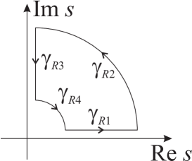
Figure 1: Integration path $\Gamma$ for zeros of $\hat{P}$

Let $\Gamma=\gamma_{R1}\cup\gamma_{R2}\cup\gamma_{R3}\cup\gamma_{R4}$ be a contour as shown in Figure 1.

Contour $\gamma_{R1}$ is parametrized by $s=x$, $x\in(\varepsilon,R)$ with $\varepsilon\to 0$, $R\to\infty$. On this part we have $\mathop{\rm Im}\nolimits\tilde{P}(s)=0$, $\mathop{\rm Re}\nolimits\tilde{P}(s)=1+x^{\alpha}(a_{2}+2b_{2}\cos(\ln x^{\beta}))\geq 1+x^{\alpha}(a_{2}-2b_{2})$. Thus, $\mathop{\rm Re}\nolimits\tilde{P}(s)\to\infty$ as $x\to\infty$ if $a_{2}>2b_{2}$, which is satisfied due to the thermodynamical restrictions (13)₂, see the end of Proposition 2.2.

Along $\gamma_{R2}$ we have $s=Re^{i\varphi}$, $\varphi\in[0,\pi/2]$, $R\to\infty$, so that

$$\mathop{\rm Re}\nolimits\tilde{P}(s) =1+a_{2}R^{\alpha}\cos(\alpha\varphi)+2b_{2}R^{\alpha}f(\ln R^{\beta},\varphi)$$

$$\mathop{\rm Im}\nolimits\tilde{P}(s) =a_{2}R^{\alpha}\sin(\alpha\varphi)+2b_{2}R^{\alpha}g(\ln R^{\beta},\varphi),$$

where $f$ and $g$ are given by (14) and (15). The minimum of $f$ is given by (24), hence $\mathop{\rm Re}\nolimits\tilde{P}(s)>1$ on $\gamma_{R2}$ if

$$a_{2}>2b_{2}\cosh\frac{\beta\pi}{2}\sqrt{1+\Big{(}\mathop{\rm tg}\nolimits\frac{\alpha\pi}{2}\mathop{\rm tgh}\nolimits\frac{\beta\pi}{2}\Big{)}^{2}}.$$

This condition is satisfied because of the dissipation inequality (12)_s. Moreover, we have

$$\mathop{\rm Re}\nolimits\tilde{P}(s) \to\infty\,\,\,\mbox{ and }\,\,\,\mathop{\rm Im}\nolimits\tilde{P}(s)\to 0,\,\,\,\mbox{ for }\,\,\,\varphi=0,\,R\to\infty,$$

$$\mathop{\rm Re}\nolimits\tilde{P}(s) \to\infty\,\,\,\mbox{ and }\,\,\,\mathop{\rm Im}\nolimits\tilde{P}(s)\to\infty,\,\,\,\mbox{ for }\,\,\,\varphi=\frac{\pi}{2},\,\alpha<1,\,R\to\infty.$$

On $\gamma_{R3}$ we have $s=ip$, $p\in(\varepsilon,R)$ with $\varepsilon\to 0$, $R\to\infty$. According to the calculated Fourier transform of $P$ and its relation with the Laplace transform, we have

$$\mathop{\rm Re}\nolimits\tilde{P}(s=ip) =1+a_{2}p^{\alpha}\cos\frac{\alpha\pi}{2}+2b_{2}p^{\alpha}f(p,\pi/2)$$

$$\geq 1+p^{\alpha}\cos\frac{\alpha\pi}{2}\bigg{(}a_{2}-2b_{2}\cosh\frac{\beta\pi}{2}\sqrt{1+\Big{(}\mathop{\rm tg}\nolimits\frac{\alpha\pi}{2}\mathop{\rm tgh}\nolimits\frac{\beta\pi}{2}\Big{)}^{2}}\bigg{)},$$

with $f$ defined by (14) and its minimal value given in (16)₁. Using (13)₂ we conclude that $\mathop{\rm Re}\nolimits\tilde{P}(s=ip)\geq 1$, for all $p\in(\varepsilon,R)$.

Finally, parametrization of $\gamma_{R4}$ is $s=\varepsilon e^{i\varphi}$, $\varphi\in[0,\pi/2]$, $\varepsilon\to 0$, so that $\mathop{\rm Re}\nolimits\tilde{P}(\varepsilon e^{i\varphi})\to 1$, $\mathop{\rm Im}\nolimits\tilde{P}(\varepsilon e^{i\varphi})\to 0$, as $\varepsilon\to 0$.

All together, the change of the argument of function $\tilde{P}$ along $\Gamma$ is zero, i.e.,

$$\Delta\arg\psi(s)=0,$$

implying that there are no zeroes of $\tilde{P}$ in the right complex half-plane. Therefore there are no singular points of $M(s)$ with $\mathop{\rm Re}\nolimits s>0$. $\Box$

The following Corollary provides that the solution (29) is well defined.

Corollary 4.2

Functions $1-exp(2sM(s)l)$ and $1-exp(-2sM(s)l)$ have no zeros in the right complex half-plane $\mathop{\rm Re}\nolimits s\geq 0$.

Proof. Zeros of functions $1-exp(2sM(s)l)$ and $1-exp(-2sM(s)l)$ satisfy $sM(s)=0$. The claim now follows from Proposition 4.1. $\Box$

Remark 4.3

Using our calculations for the Fourier transformation of $E$, we have

$$M^{2}(i\omega)=\frac{1}{\hat{E}(\omega)}=\frac{\mathop{\rm Re}\nolimits\hat{E}(\omega)-i\mathop{\rm Im}\nolimits\hat{E}(\omega)}{|\hat{E}(\omega)|^{2}},$$

and $\mathop{\rm Re}\nolimits\hat{E}(\omega),\mathop{\rm Im}\nolimits\hat{E}(\omega)\geq 0$ for $\omega>0$, we conclude that $\mathop{\rm Re}\nolimits M^{2}(i\omega)>0$ and $\mathop{\rm Im}\nolimits M^{2}(i\omega)<0$ for $\omega>0$ if the thermodynamical restrictions (11), (12)_s and (13) are satisfied. Hence $\mathop{\rm Re}\nolimits M(i\omega)>0$ and $\mathop{\rm Im}\nolimits M(i\omega)<0$, $\omega>0$. Also, from Remark 3.2, it follows $\mathop{\rm Re}\nolimits M(-i\omega)>0$ and $\mathop{\rm Im}\nolimits M(-i\omega)<0$, $\omega>0$.

Similarly, from

$$M^{2}(s)=\frac{1}{\hat{E}(s)}=\frac{\mathop{\rm Re}\nolimits\hat{E}(s)-i\hat{E}(s)}{|\hat{E}(s)|^{2}}$$

and Proposition 3.1 we conclude that $\mathop{\rm Re}\nolimits M^{2}(s)>0$, $s=s_{0}+ip$, $s_{0},p>0$, and $\mathop{\rm Im}\nolimits M^{2}(s)\leq 0$, $s=s_{0}+ip$, $s_{0}>0$, $p>p_{0}$. Consequently, $\mathop{\rm Re}\nolimits M(s)>0$, $s=s_{0}+ip$, $s_{0},p>0$, and $\mathop{\rm Im}\nolimits M(s)<0$, $s=s_{0}+ip$, $s_{0}>0$, $p>p_{0}$.

We now state the main result of this Section.

Theorem 4.4

Problem (7)-(8) has a solution given as

$$u(x,t)=(U\ast_{t}K)(x,t)=\int_{0}^{t}U(t-\tau)K(x,\tau)\,d\tau,\quad x\in(0,l],\,\,\,t>0,$$ (31)

where, for $l=\infty,$

$$K(x,t)=\frac{1}{2\pi i}\int_{s_{0}-i\infty}^{s_{0}+i\infty}\exp(ts)\Big{[}\frac{\exp(sM(s)x)}{1-exp(2sM(s)l)}+\frac{\exp(-sM(s)x)}{1-exp(-2sM(s)l)}\Big{]}\,ds,$$

or

$$K(x,t)=\frac{1}{2\pi i}\int_{s_{0}-i\infty}^{s_{0}+i\infty}\exp(ts)\exp(-sM(s)x)\,ds$$ (32)

if $l=\infty$. Here $s_{0}>0$. In particular, for every $t$, $K$ is continuous with respect to $x$, as well as $u$. If $x=0$ then $K(0,t)=\delta(t)$.

In the case $l=\infty$ solution (31) can be computed more explicitly, as it is given in the following statement.

Theorem 4.5

Let $l=\infty$. Then the solution kernel (32) takes the form

$$K(x,t)=\frac{1}{\pi}\int_{0}^{\infty}\exp\big{[}\tau\mathop{\rm Im}\nolimits M(i\tau)x\big{]}\cos\big{[}\tau(t-\mathop{\rm Re}\nolimits M(i\tau)x)\big{]}\,d\tau,\quad x>0,\,\,\,t>0.$$ (33)

It is continuous function of $x$. If $x=0$ then $K(0,t)=\delta(t)$.

Proof. Set $s=s_{0}+i\tau$ ($ds=i\,d\tau$) and $p>0$. Then (32) becomes

$$K(x,t)=\frac{1}{2\pi i}\lim_{p\to\infty}\int_{-p}^{p}\exp\big{[}(s_{0}+i\tau)(t-M(s_{0}+i\tau)x)\big{]}\,d\tau,\quad x>0,\,\,\,t>0.$$

The estimate below shows the continuity with respect to $x>0$ for every $t>0$.

Consider the contour shown in Figure 2. Then $K(x,t)=\frac{1}{2\pi}\lim_{p\to\infty}I_{1}(x,t,p)$, $x\geq 0$, $t>0$, where the Cauchy integral theorem implies

$$I_{1}=-(I_{2}+I_{3}+I_{4}+I_{5}+I_{6}).$$

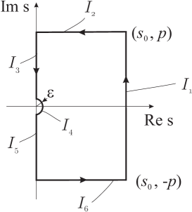
Figure 2: Integration path $I$

For the integral $I_{2}$ we have to use (23) and

$$|I_{2}| =\Big{|}-\int_{0}^{s_{0}}\exp\big{[}(\sigma+ip)(t-M(\sigma+ip)x)\big{]}\,d\sigma\Big{|}$$

$$\leq\int_{0}^{s_{0}}\exp\big{[}\sigma(t-\mathop{\rm Re}\nolimits M(\sigma+ip)x)+p\mathop{\rm Im}\nolimits M(\sigma+ip)x\big{]}\,d\sigma$$

$$\leq C\,\int_{0}^{s_{0}}\exp\big{[}p\mathop{\rm Im}\nolimits M(\sigma+ip)\big{]}\,d\sigma$$

$$\leq C\,\int_{0}^{s_{0}}\exp\big{[}-p^{1+\frac{\alpha}{2}}\big{]}\,d\sigma$$

$$<\infty$$

Similar arguments prove that $\lim_{p\to\infty}I_{6}=0$.

Next for $I_{4}$ we have $s=\varepsilon\exp(i\varphi)$, $ds=i\varepsilon\exp(i\varphi)\,d\varphi$ so that

$$\lim_{\varepsilon\to 0}I_{4}=\lim_{\varepsilon\to 0}\int_{-\pi/2}^{\pi/2}\exp\big{[}\varepsilon\exp(i\varphi)(t-M(\varepsilon\exp(i\varphi))x)\big{]}i\varepsilon\exp(i\varphi)\,d\varphi=0.$$

Therefore $I_{1}=-(I_{3}+I_{5})$ so that with $s=i\tau$ we get

$$I_{1} =-i\Big{[}\int_{p}^{\varepsilon}\exp\big{[}i\tau(t-M(i\tau)x)\big{]}\,d\tau+\int_{-\varepsilon}^{-p}\exp\big{[}i\tau(t-M(i\tau)x)\big{]}\,d\tau\Big{]}$$

$$=-2i\Big{[}\int_{p}^{\varepsilon}\exp\big{[}\tau\mathop{\rm Im}\nolimits M(i\tau)x\big{]}\cos\big{[}\tau(t-\mathop{\rm Re}\nolimits M(i\tau)x)\big{]}\,d\tau\Big{]},$$

where we used $\mathop{\rm Im}\nolimits M(-ip)=-\mathop{\rm Im}\nolimits M(ip)$, $\mathop{\rm Re}\nolimits M(ip)=\mathop{\rm Re}\nolimits M(-ip)$. Thus,

$$K(x,t)=\frac{1}{\pi}\lim_{\varepsilon\to 0}\Big{(}\lim_{p\to\infty}\int_{\varepsilon}^{p}\exp\big{[}\tau\mathop{\rm Im}\nolimits M(i\tau)x\big{]}\cos\big{[}\tau(t-\mathop{\rm Re}\nolimits M(i\tau)x)\big{]}\,d\tau\Big{)},\quad x>0,\,\,\,t>0,$$

which proves the claim. $\Box$

Remark 4.6

In the numerical example of the last Section we can notify an oscillatory character of the solution which comes from integrals $I_{2}$ and $I_{6}$ that is obtained in numerical experiments for relatively small values of $p$ (see the next Section 5).

5 Numerical experiments

Results obtained in previous sections will be presented for various sets of parameters and boundary conditions. The goal is to examine and compare how different values of coefficients and orders of fractional derivatives influence the solution, i.e., how the solution wave propagates in the viscoelastic rod. We treat two different cases:

Case 1. Choose the following values for the parameters in system (7)-(8)

$$a_{1}=1,\quad a_{2}=20,\quad b_{1}=0.1,\quad l=\infty.$$

Then according to (11), $b_{2}=a_{2}b_{1}/a_{1}=2$, and one checks easily, by inserting these chosen values of parameters into (12) and (13), that the thermodynamical restrictions are satisfied. Suppose that $U(t)=\delta(t)$, the Dirac distribution. Then combining (31) and (33) the solution reads

$$u(x,t)=\frac{1}{\pi}\int_{0}^{\infty}\exp\big{[}\tau\mathop{\rm Im}\nolimits M(i\tau)x\big{]}\cos\big{[}\tau(t-\mathop{\rm Re}\nolimits M(i\tau)x)\big{]}\,d\tau.$$ (34)

In Figure 3 we present solution $u$ given by (34) for $\alpha=0.5$, $\beta=0.1$ and $t=1$.

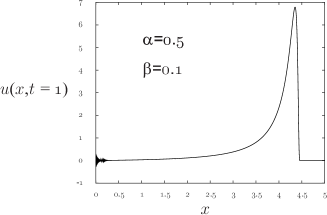
Figure 3: Displacement $u$ for $\alpha=0.5$, $\beta=0.1$ and $t=1$.

In order to examine the influence of $\alpha$ on the solution, in Figure 4 we present $u$ given by (34) for $\alpha=0.7$, $\beta=0.1$ and $t=1$.

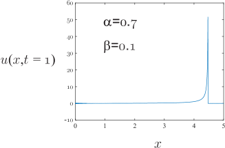
Figure 4: Displacement $u$ for $\alpha=0.7$, $\beta=0.1$ and $t=1$.

Finally, we increase $\beta$, so we consider the case $\alpha=0.5$, $\beta=0.3$ and $t=1$. The results are shown in Figure 5.

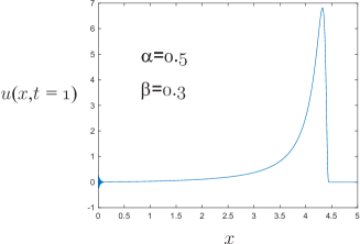
Figure 5: Displacement $u$ for $\alpha=0.5$, $\beta=0.3$ and $t=1$.

Case 2. Suppose now that $U(t)=H(t)$, where $H$ is the Heaviside function. Also, we assume that the parameters are chosen so that thermodynamical (12) and (13) are satisfied. Using (31) and (33) we obtain

$$u(x,t)=\frac{1}{\pi}\int_{0}^{t}\Big{[}\int_{0}^{\infty}\exp\big{[}\tau\mathop{\rm Im}\nolimits M(i\tau)x\big{]}\cos\big{[}\tau(\theta-\mathop{\rm Re}\nolimits M(i\tau)x)\big{]}\,d\tau\Big{]}\,d\theta.$$ (35)

For $x=0$ from (35) we obtain

$$u(0,t)=\frac{1}{\pi}\int_{0}^{t}\int_{0}^{\infty}\cos(\tau\theta)\,d\tau\,d\theta.$$

By using the fact that Dirac $\delta$ function may be approximated as

$$\delta(\xi)=\frac{1}{\pi}\lim_{\nu\to 0}\int_{0}^{1/\nu}\cos(\tau\theta)\,d\tau,$$

we obtain

$$u(0,t)=1.$$

Thus the boundary condition $u(0,t)=H(t)$ is satisfied.

6 Conclusion

In this work we proposed a constitutive equation for viscoelastic body of generalized Zener type that includes fractional derivatives of stress and strain of real and complex order. With such constitutive equation, the initial-boundary value problem that generalizes the classical wave equation is given by (7)-(8). Note that for the case $a_{1}=b_{1}=a_{2}=b_{2}=0$ the constitutive equation (1)₂ becomes Hooke’s law, and (7)-(8) reduces to an initial-boundary value problem for the classical wave equation.

The results of this paper may be summarized as follows:

1. We formulated initial-boundary value problem for the generalized wave equation in the viscoelastic body described by fractional derivatives of real and complex order in the form (7)-(9).

2. We determined restrictions on the coefficients from the dissipativity conditions in the form (11), (12) and (13), and later in a strong form, for the sake of solvability. We concluded that dissipativity conditions, that are consequences of the Second Law of Thermodynamics for isothermal deformation in a strong form (11), (12)_s and (13)_s, guarantee the solvability of the constitutive equation (1)₂ for $\sigma$ and $\varepsilon$.

3. We presented the solution to (7)-(8) in the form of (31).

4. We analyzed two specific examples. In the first example the solution is given by (34). For the Dirac delta impulse as the boundary condition, the solution shows a pulse behavior that dissipates with time. In calculating the integral in (34) there was observed oscillation type behavior for small times. We attribute this behavior to the imaginary order term in the derivation since for small $p$ the influence of oscilating factor in the integrals $I_{2},I_{6}$ is evident.

5. Further study is needed to examine the influence of parameters of the model and order of derivatives on the properties of the solution.

References

[1]
Amendola, G., Fabrizio, M., Golden, J. M.
Thermodynamics of Materials with Memory.
Springer, New York, 2012.
[2]
Atanacković, T.M.
A modified Zener model of viscoelastic body.
Contin. Mech. Thermodyn., 14:137–148, 2002.
[3]
Atanacković, T.M., Janev, M., Konjik, S., Pilipović, S., Zorica, D.
Vibrations of an elastic rod on a viscoelastic foundation of complex
fractional kelvin-voigt type.
Meccanica, 50(7):685–704, 2015.
[4]
Atanacković, T.M., Konjik, S., Oparnica, Lj., Zorica, D.