Solving generalized maximum-weight connected subgraph problem for network enrichment analysis

Abstract

Network enrichment analysis methods allow to identify active modules without being biased towards a priori defined pathways. One of mathematical formulations of such analysis is a reduction to a maximum-weight connected subgraph problem. In particular, in analysis of metabolic networks a generalized maximum-weight connected subgraph (GMWCS) problem, where both nodes and edges are scored, naturally arises. Here we present the first to our knowledge practical exact GMWCS solver. We have tested it on real-world instances and compared to similar solvers. First, the results show that on node-weighted instances GMWCS solver has a similar performance to the best solver for that problem. Second, GMWCS solver is faster compared to the closest analogue when run on GMWCS instances with edge weights.

1 Introduction

Gene set enrichment methods are widely used for the analysis of untargeted biological data such as transcriptomic, proteomic or metabolomic profiles. These methods allow to identify molecular pathways, in a form of gene sets, that have non-random group behaviour in the data. Determining such overenriched pathways provides insights into the data and allows to better understand the considered system.

Network enrichment methods, in opposite to gene set enrichment, do not rely on the predefined gene sets and, thus, allow to identify novel pathways. These methods use network of interacting entities, such as genes, proteins, metabolites, etc. and try to identify the most regulated subnetwork. There are different mathematical formulations of the network enrichment problem, but many of them are NP-hard [8, 5, 1].

Dittrich et al. in [5] suggested a formulation as a maximum-weight connected subgraph (MWCS) problem. Originally, the authors considered node-weighted graph, such that positive weight corresponded to ”interesting” nodes and negative weight corresponded to ”non-interesting” nodes. The goal was to find a connected graph with the maximal sum of weights of its nodes, which corresponded to an ”active module”.

Here we consider, a slightly different form of MWCS, generalized MWCS (GMWCS), that has edges also weighted. Such formulation naturally arises in the studies of metabolic networks [4, 9], where nodes in the graph represent metabolites and edges represent their interconversions via reactions. There, the nodes can be scored using metabolomic profiles and the edges can be scored using gene or protein expression profiles.

In this paper we describe an exact solver for the node-and-edge-weighted GMWCS problem. First, in section 2 we give formal definitions. Then in section 3 we describe preprocessing steps adapted for the edge-based formulation. In section 4 we show how the instance can be split into three smaller instances. Section 5 is dedicated to a mixed-integer programming (MIP) formulation of the problem. In section 6 we show experimental results of running the solver on real-world instances that appear in GAM web-service and show that it is faster and more accurate than Heinz [3] on edge-weighted instances and is similar in performance to Heinz2 [6] on node-weighted instances.

2 Formal definitions

Here we consider the Maximum-Weight Connected Subgraph (MWCS) problem for which there are two slightly different formulations. In the most commonly used definition of MWCS only nodes are weighted [2, 6]. In this paper we consider problem where edges are weighted too [7]. To remove the ambiguity we call the former problem Simple MWCS (SMWCS) and the latter one Generalized MWCS (GMWCS).

The goal of MWCS problems is to find in a given graph a connected subgraph with the maximal the maximal sum of weights. As a subgraph is connected we can consider connected components of the graph independently. Thus, below we assume that the input graph is connected.

First, we give definition of a Simple Maximum-Weight Connected Subgraph problem.

Definition 1

Given a connected undirected graph $G=(V,E)$ and weight function $\omega_{v}:V\rightarrow\mathbb{R}$, the Simple Maximum-Weight Connected Subgraph (SMWCS) problem is the problem of finding a connected subgraph $\widetilde{G}=(\widetilde{V},\widetilde{E})$ with the maximal total weight

$$\Omega(\widetilde{G})=\sum_{v\in\widetilde{V}}\omega(v)\rightarrow max$$

Second, we define generalized variant of this problem, where both nodes and edges could be weighted.

Definition 2

Given a connected undirected graph $G=(V,E)$ and a weight function $\omega:(V\cup E)\rightarrow\mathbb{R}$, the Generalized Maximum-Weight Connected Subgraph (GMWCS) problem is the problem of finding a connected subgraph $\widetilde{G}=(\widetilde{V},\widetilde{E})$ with the maximal total weight

$$\Omega(\widetilde{G})=\sum_{v\in\widetilde{V}}\omega(v)+\sum_{e\in\widetilde{E}}\omega(e)\rightarrow max$$

Now we define a rooted variant of the problem with one of the vertices forced to in a solution. It is used as an auxiliary subproblem of GMWCS.

Definition 3

Given a connected undirected graph $G=(V,E)$, a weight function $\omega:(V\cup E)\rightarrow\mathbb{R}$ and a root node $r\in V$ the Rooted Generalized Maximum-Weight Connected Subgraph (R-GMWCS) problem is the problem of finding a connected subgraph $\widetilde{G}=(\widetilde{V},\widetilde{E})$ such that $r\in\widetilde{V}$ and

$$\Omega(\widetilde{G})=\sum_{v\in\widetilde{V}}\omega(v)+\sum_{e\in\widetilde{E}}\omega(e)\rightarrow max$$

El-Kebir et al. in [6] have shown that MWCS problem is NP-hard. Since MWCS is a special case of GMWCS then GMWCS is also NP-hard. R-GMWCS problem is NP-hard too because any instance of GMWCS problem can be solved by solving an R-GMWCS instance for each node as a root.

Finally, below we use $n$ as a shorthand for the number of nodes $|V|$ in the graph $G$.

3 Preprocessing

We introduce two preprocessing rules adapted from [6] that simplify the problem. These rules make a new graph with a smaller number of vertices and edges in such a way that the GMWCS solution for the original graph can be easily recovered from the GMWCS solution for the simplified graph.

First, we merge groups of close vertices that either none or all of them are in the optimal solution (Fig. 1A). Let $e=(u,v)$ be an edge with $\omega(e)\geq 0$ with simultaneously $\omega(e)+\omega(v)\geq 0$ and $\omega(e)+\omega(u)\geq 0$. In this case if one of the vertices is included in the solution then the edge and the other vertex can also be included without decreasing the total weight. Thus, we can contract edge $e$ into a new vertex $w$ with a weight $\omega(w)=\omega(e)+\omega(u)+\omega(v).$ After the contraction parallel edges between $w$ and some vertex $t$ could appear. In that case we merge all non-negative one into a single edge with weight of the sum of their weights. After that, we remove all edges between $w$ and $t$ except one with the maximal weight. We try to apply this rule for all vertices in the loop while the graph is changing.

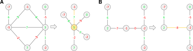
Figure 1: Applying first rule that contract an edge (A) and second rule that replace negative chain by a single edge (B). New vertices and nodes painted yellow

Second, similarly to the previous step, we merge negative-weighted chains (Fig. 1B). Let $v$ be a vertex with $deg(v)=2$ with corresponding incident edges $e_{1}=(u,v)$ and $e_{2}=(v,w)$. If all three weights $\omega(v)$, $\omega(e_{1})$ and $\omega(e_{2})$ are negative, then $v$, $e_{1}$ and $e_{2}$ could be replaced with a single edge $e=(u,w)$ with a weight $\omega(e)=\omega(v)+\omega(e_{1})+\omega(e_{2})$. Merging negative chains is implemented in a single pass by iteratively trying to apply the rule for all the nodes.

4 Cut vertex decomposition

In this section we discuss how a GMWCS instance can be decompose into three smaller problems. The decomposition is based on the idea that biconnected components can be considered separately [6].

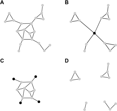
Figure 2: Input graph and instances spawned by decomposition

Briefly, we have a GMWCS instance as input (Fig. 2A). First, we merge the largest biconnected component into a single vertex with zero weight and solve an R-GMWCS instance for this modified graph and the new vertex as a root (Fig. 2B). Then, we replace each of the components branching from the largest biconnected component by a single vertex with weight equal to the weight of corresponding subgraph in the R-GMWCS solution from the previous step (Fig. 2C). Last, we try to find a subgraph with a greater weight which fully lies in one of the branching components (Fig. 2D).

Formally, let $B$ be a biconnected component of the graph $G$ with the maximal number of vertices. Let $C$ be a set of cut vertices of the graph $G$ that are also contained in $B$. Let $B_{c}$ be a component containing $c$ in the graph $G\setminus(B\setminus C)$.

Proposition 1

Let a subgraph $\widetilde{G}$ of $G$ be an optimal solution of GMWCS for graph $G$ and $\widetilde{G}_{c}$, $\forall c\in C$, are optimal solutions for R-GMWCS instances for graphs $B_{c}$ with a root $c$. In this case, if $\widetilde{G}$ contains a vertex $c\in C$, then we can construct an optimal solution $\widetilde{G}^{\prime}$ such that: 1) $\widetilde{G}^{\prime}\cap B$ = $\widetilde{G}\cap B$ and 2) $\widetilde{G}^{\prime}\cap B_{c}=\widetilde{G}_{c}$.

Proof

Let $\widetilde{B}_{c}=\widetilde{G}\cap B_{c}$. We prove that it can be replaced by $\widetilde{G}_{c}$ without loss of connectivity and optimality. First, $\widetilde{B}_{c}$ must be connected. Let it be disconnected. Then there is no path between $c$ and some vertex $v$. Since $\widetilde{G}$ is connected then there is a simple path $vc$ in $G$. However, by definition of cut vertex, path $vc$ can not contain vertices from $G\setminus B_{c}$ and, thus it fully lies in $B_{c}$, a contradiction. Since $\widetilde{B}_{c}$ is connected and contains $c$ then it cannot have weight greater than $\widetilde{G}_{c}$ by construction of $\widetilde{G}_{c}$.

Now we prove that the replacement keeps the graph connected. Repeating the reasoning from the previous step we can get that $\widetilde{G}\cap B$ must be connected. So, $\widetilde{G}_{c}$ is connected, $\widetilde{G}\cap B$ connected and both these graphs contain $c$. Thus, $\widetilde{G}^{\prime}$ is also connected. $\square$

This proposition allows us to consider only optimal solutions that either include a vertex from $B$ and in subgraphs $B_{c}$ are identical to the corresponding R-GMWCS instance or fully lie in some of the subgraphs $B_{c}$.

First, for each $c\in C$ we want to know the best solution of the problem for the graph $B_{c}$ containing vertex $c$. It is precisely an R-GMWCS instance. For practical reasons, it is better to spawn one instance at this step instead of $|C|$ instances. Let $G^{*}=\bigcup_{\forall c\in C}B_{c}$. Then we merge all vertices from $C$ contained in $G^{*}$ into a single vertex $r$ with $\omega(r)=0$ and solve R-GMWCS problem for such graph. Let $S$ to be the solution of this instance. To get solution for the graph $B_{c}$ we replace back $r$ to $c$ in $S$, and remove all the vertices which are not contained in $B_{c}$.

Second, we find best scored subgraph of $G$ that do not lies fully in some of $B_{c}$. Let $\widetilde{G}_{c}$ be the solution of R-GMWCS for graph $B_{c}$ with root $c$ obtained on the previous step. We obtain a new GMWCS instance by considering the component $B$ and for all $c\in C$ attaching a vertex $v$ with weight $\omega(v)=\Omega(\widetilde{G}_{c})$. We solve the resulting instance and then recover a solution for the original problem.

Last, we find all potential solutions that fully lie in $B_{c}$ for all $c\in C$. For this purpose we spawn one instance for the graph $G^{*}=\bigcup_{\forall c\in C}B_{c}$. Clearly that if the solution of the problem for the graph $G$ lies fully in some of $B_{c}$ then we will find it at this step.

5 Mixed integer programming formulation

Here we describe a MIP formulation of the problem. The GMWCS can be represented as two parts: objective function (weight of the subgraph) that should be maximized and constraints that ensure that the subgraph is connected. The objective function is linear and can be put into a MIP problem in a straightforward way. However, getting effective linear subgraph connectivity constraints is not trivial. In this section we describe how it can be done. The resulting MIP problem is solved by IBM ILOG CPLEX.

First, we consider a nonlinear formulation of the GMWCS problem, as proposed in [7]. Then, we show how to eliminate nonlinearity and get a linear system. Finally, we introduce extra symmetry-breaking and cuts, which do not impact on the correctness of the formulation, but improve the performance.

5.1 Subgraph representation

We use one binary variable for each vertex or edge that represent the presence in the subgraph:

1. Binary variable $y_{v}$ takes the value of 1 iff $v\in V$ belongs to the subgraph.

2. Binary variable $w_{e}$ takes the value of 1 iff $e\in E$ belongs to the subgraph.

For these variables to be representing a valid subgraph (not necessarily connected) we need to introduce a set of constraints:

$$w_{e} \leq y_{v}, \forall v\in V,e\in\delta_{v}.$$ (1)

These constraints state that an edge can be a part of the subgraph, only if both of its endpoints are a part of the subgraph.

5.2 Nonlinear formulation

The nonlinear formulation of the subgraph connectivity constraints is based on the idea that any connected graph can be traversed from any of its vertices. The output of the traversal can be represented as an arborescence where an arc $(v,u)$ denotes that $v$ has been visited before $u$. Accordingly, we can ensure connectivity of a subgraph if we can provide an arborescence corresponding to the traversal of this subgraph.

For a given graph $G=(V,E)$, let $S=(V,A)$ be a directed graph, where $A$ is obtained from $E$ by replacing each undirected edge $e=(v,u)$ by two directed arcs $(v,u)$ and $(u,v)$.

Now, we are going to introduce variables that we will use in the formulation and show nonlinear system of constraints, that ensure connectivity of subgraph:

1. Binary variable $x_{a}$ takes the value of 1 iff $a\in A$ belongs to the arborescence.

2. Binary variable $r_{v}$ takes the value of 1 iff $v\in V$ is the root of the arborescence.

3. Continuous variable $d_{v}$ takes the value of $n$ if the path in the arborescence from the root to vertex $v$ contains $n$ vertices. If $v$ does not belong to the solution then value can be arbitrary.

Then we introduce constraints that ensure the validity of an arborescence:

$$\sum_{v\in V}r_{v} =1;$$ (2)

$$1\leq d_{v} \leq n, \forall v\in V;$$ (3)

$$\sum_{(u,v)\in A}x_{uv}+r_{v} =y_{v}, \forall v\in V;$$ (4)

$$x_{vu}+x_{uv} \leq w_{e}, \forall e=(v,u)\in E;$$ (5)

$$d_{v}r_{v} =r_{v}, \forall v\in V;$$ (6)

$$d_{u}x_{vu} =(d_{v}+1)x_{vu}, \forall(v,u)\in A.$$ (7)

Inequality (2) states that there is only one root in the arborescence; (3) is a limitation on the distance between any vertex and the root; (4) states that if a vertex is a part of the subgraph then either it is a root of the arborescence or $deg_{in}(v)=1$; (5) says that an arc of the arborescence can be in the solution only if the corresponding edge is also in it. Last two inequalities (6) and (7) control correct distances in the arborescence.

Haouari et al. have shown in [7] that this nonlinear system is a correct formulation of GMWCS. That is, the arborescence covers all vertices of the resulting subgraph and the solution can induce this arborescence.

However, inequalities (6) and (7) are not linear and should be replaced, so that the formulation can be represented as a MIP problem.

5.3 Linearization

Nonlinear equations (6) and (7) can be replaced with the following system of linear inequalities:

$$d_{v}+nr_{v} \leq n, \forall v\in V;$$ (8)

$$n+d_{u}-d_{v} \geq(n+1)x_{vu}, \forall(v,u)\in A;$$ (9)

$$n+d_{v}-d_{u}+ \geq(n-1)x_{vu}, \forall(v,u)\in A.$$ (10)

Proposition 2

Every feasible solution to (1)-(7) is also feasible to (1)-(5), (8)-(10) and vice versa.

Proof

First, we prove that (8) is equivalent to (6) in a sense of feasibility of the solution. Since $r_{v}$ is a binary variable, we can consider two cases. Suppose that $r_{v}=1$, then (6) will take the form $d_{v}=1$ while (8) will take the from $d_{v}\leq 1$, and with (3) we have $d_{v}=1$. Now suppose that $r_{v}=0$, (6) will look $0=0$, it means that in this case there is no additional restrictions on variables and (8) will take the form $d_{v}\leq n$, but system already have such inequality. Thus (6) and (8) are equivalent for both possible values of $r_{v}$.

At the second part of the proof we will use the same approach. Here we prove that (7) can be represented as linear inequalities (9) and (10).

1. Let $x_{vu}=1$. Then after substitution into (7) we have $d_{u}=d_{v}+1$. Then we substitute $x_{vu}$ into (9) and (10)

   $$n+d_{u}-d_{v}\geq n+1$$

   $$n+d_{v}-d_{u}\geq n-1$$

   or, equivalently,

   $$d_{u}\geq d_{v}+1$$

   $$d_{v}+1\geq d_{u}$$

   or $d_{u}=d_{v}+1$.

2. Let $x_{vu}=0$. The original nonlinear equation will take the form $0=0$. As mentioned above, it means that there is no additional restrictions on variables. We have to show that (9) and (10) also do not add such restrictions. After substitution these inequalities take the form:

   $$n+d_{u}-d_{v}\geq 0$$

   $$n+d_{v}-d_{u}\geq 0$$

   or $|d_{v}-d_{u}|\leq n$. Obviously, variables that hold (3) automatically hold such inequality. Thus, additional restrictions have not be added. $\square$

5.4 Symmetry-breaking

It is a common practice to decrease the number of feasible solutions by limiting the number of different but logically equivalent feasible solutions. Such solutions are called symmetric. In our formulation constraints (1)-(5), (8)-(10) allow any arborescence of the graph to show its connectivity. So, in this section we show how to decrease the number of feasible arborescences and thus decrease the search space.

5.4.1 Root order rule.

First of all, for the unrooted GMWCS problem we force the arborescence root to be a vertex with the maximal weight among present in the subgraph. Corresponding constraint that is added in the MIP instance is:

$$\sum_{v\prec u}r_{v} \leq 1-y_{u}, \forall u\in V,$$ (11)

where $v\prec u$ if $\omega(v)<\omega(u)$ or if weights are equal, we use some fixed linear order on vertices.

For the R-GMWCS we set root of the arborescence to be the same as the instance root.

5.4.2 Restricting traversal.

Moreover, connected graph can be traversed from the same vertex in different ways. In this section we show how to make infeasible such solutions that could not be reached by a breadth-first search (BFS).

To achieve such form of the arborescence we add constraints:

$$d_{v}-d_{u} \leq n-(n-1)w_{e}, \forall e=(v,u)\in E;$$ (12)

$$d_{u}-d_{v} \leq n-(n-1)w_{e}, \forall e=(v,u)\in E.$$ (13)

These constraints state that if an edge $e$ is present the subgraph then the distances to endpoints differ by one.

Proposition 3

For any connected subgraph $G_{s}$ of the graph $G$ there exists a solution $(\overline{r},\overline{y},\overline{w},\overline{x},\overline{d})$ that encodes subgraph $G_{s}$ and is feasible to (1)-(5), (8)-(10) and (11)-(13).

Proof

First, for any subgraph $G_{s}$ we can select any of its vertices, in particular one with the maximal weight, and make a BFS traversal starting from that vertex. As was shown above for any connected subgraph $G_{s}$ and any its arborescence there is a corresponding encoding $(\overline{r},\overline{y},\overline{w},\overline{x},\overline{d})$ that satisfy constraints (1)-(5) and (8)-(10). By selection of the vertex with the maximal weight as an arborescence root constraint (11) holds. Constraints (12)-(13) also hold as they directly follow from the BFS ordering. $\square$

5.5 Extra cuts

We also use additional cuts, similar to ones proposed by Álvarez-Miranda et al. in [2]. However we modified them for applying in edge-based R-GMWCS problem. Such cuts are useful for decreasing the upper bound of the objective of the MIP problem that solving using brunch and cut algorithm.

So, we use cut constraints of the form:

$$y_{v} \leq\sum_{e\in C}w_{e}, \forall v\in V,C\in C^{*},$$ (14)

where $C^{*}$ is a set of all cuts between instance root and vertex $v$. To find violated inequalities we associate with each edge $e$ the LP relaxation value of the variable $w_{e}$ and for each vertex $v$ we try to find violated constraint by looking for the cut $C$ such that $y_{v}>\sum_{e\in C}w_{e}$. The minimum cut is the best candidate of constraint being violated. So, we use the Edmonds-Karp algorithm to find such violated constraints.

6 Experimental results

As a testing dataset we used 101 instance generated by Shiny GAM, a web-service for integrated transcriptional and metabolic network analysis [9]. In the dataset, there are 38 instances of node-weighted SMWCS and 63 instances of GMWCS. Archive with instances is available at http://genome.ifmo.ru/files/papers_files/WABI2016/gmwcs/instances.tar.gz.

For the comparison we selected two other solvers: Heinz version 1.68 [5] and Heinz2 version 2.1 [6]. The first one, Heinz, was initially developed for node-weighted SMWCS, but later was adjusted to account for edge weights, however, only acyclic solutions are considered. The second one, Heinz2, does not accept edge weights, but works faster than Heinz on node-weighted instances.

We ran each of the solver on each of the instances for 10 times with a time limit of 1000 seconds. Heinz2 and our GMWCS solver were run using 4 threads. The processor was AMD Opteron 6380 2.5GHz. A table with the results table are available at http://genome.ifmo.ru/files/papers_files/WABI2016/gmwcs/results.final.tsv.

6.1 Results for simple MWCS

The experiments have shown that on the node-weighted instances GMWCS solver has a performance similar to Heinz2 (Fig. 3A). For 24 instances (63%) GMWCS is slower than Heinz2. However, 32 instances (84%) were solved by GMWCS within 30 seconds, compared to 27 (71%) of Heinz2. Moreover, 4 instances were not solved by Heinz2 in the allowed time of 1000 seconds compared to only 1 instance for GMWCS.

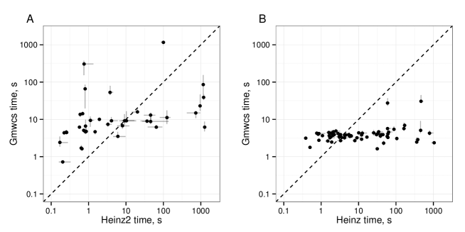
Figure 3: Comparison of GMWCS with Heinz2 and Heinz solvers on node-weighted (A) and node-and-edge-weighted (B) instances. The points represent median times of 10 runs on one instance. Horizontal and vertical grey lines represent the second minimal and the second maximal times. For convenience a small random noise was added to the median values of more then 950 seconds.

6.2 Results for generalized MWCS

For the edge-weighted GMWCS instances GMWCS solver was able to find optimal solutions within 10 seconds all instances except two, while it took for Heinz more than 10 seconds to solve 30 of the instances (48%) (Fig. 3B). Moreover, only 35 instances (56%) had an acyclic solution, accordingly, 28 instances were not solved to GMWCS-optimality by Heinz.

7 Conclusion

Network analysis approaches are being actively developed for analyzing biological data. From the mathematical point of view this usually correspond to NP-hard problems. Here we described an exact practical solver for a particular formulation of generalized maximum weight connected subgraph problem that naturally arises in metabolic networks. We have tested the method on the real-world data and have shown that the developed solver is similar in performance to an existing solver Heinz2 on a simple MWCS instances and works better and more accurately compared to Heinz on the edge-weighted instances. The implementation is freely available at https://github.com/ctlab/gmwcs-solver.

Funding

This work was supported by Government of Russian Federation [Grant 074-U01 to A.A.S., A.A.L.].

References

- [1] Alcaraz, N., Pauling, J., Batra, R., Barbosa, E., Junge, A., Christensen, A.G.L., Azevedo, V., Ditzel, H.J., Baumbach, J.: KeyPathwayMiner 4.0: condition-specific pathway analysis by combining multiple omics studies and networks with Cytoscape. BMC systems biology 8(1), 99 (2014)
- [2] Álvarez-Miranda, E., Ljubić, I., Mutzel, P.: The maximum weight connected subgraph problem. In: Facets of Combinatorial Optimization, pp. 245–270. Springer (2013)
- [3] Beisser, D., Brunkhorst, S., Dandekar, T., Klau, G.W., Dittrich, M.T., Müller, T.: Robustness and accuracy of functional modules in integrated network analysis. Bioinformatics (Oxford, England) 28(14), 1887–94 (2012)
- [4] Beisser, D., Grohme, M.A., Kopka, J., Frohme, M., Schill, R.O., Hengherr, S., Dandekar, T., Klau, G.W., Dittrich, M., Müller, T.: Integrated pathway modules using time-course metabolic profiles and EST data from Milnesium tardigradum. BMC Syst Biol 6, 72 (2012)
- [5] Dittrich, M.T., Klau, G.W., Rosenwald, A., Dandekar, T., Müller, T.: Identifying functional modules in protein-protein interaction networks: an integrated exact approach. Bioinformatics (Oxford, England) 24(13), i223–31 (2008)
- [6] El-Kebir, M., Klau, G.W.: Solving the maximum-weight connected subgraph problem to optimality (2014)
- [7] Haouari, M., Maculan, N., Mrad, M.: Enhanced compact models for the connected subgraph problem and for the shortest path problem in digraphs with negative cycles. Computers & Operations Research 40(10), 2485–2492 (2013)
- [8] Ideker, T., Ozier, O., Schwikowski, B., Siegel, A.F.: Discovering regulatory and signalling circuits in molecular interaction networks. Bioinformatics (Oxford, England) 18 Suppl 1, S233–S240 (2002)
- [9] Sergushichev, A., Loboda, A., Jha, A., Vincent, E., Driggers, E., Jones, R., Pearce, E., Artyomov, M.: Gam: a web-service for integrated transcriptional and metabolic network analysis. Nucleic acids research (2016)