Fast Bilateral Filtering of Vector-Valued Images

Abstract

In this paper, we consider a natural extension of the edge-preserving bilateral filter for vector-valued images. The direct computation of this non-linear filter is slow in practice. We demonstrate how a fast algorithm can be obtained by first approximating the Gaussian kernel of the bilateral filter using raised-cosines, and then using Monte Carlo sampling. We present simulation results on color images to demonstrate the accuracy of the algorithm and the speedup over the direct implementation.

Index Terms—  Bilateral filter, vector-valued image, color image, Monte Carlo method, approximation, fast algorithm.

1 Introduction

The bilateral filter was proposed by Tomasi and Maduchi [1] as a non-linear extension of the classical Gaussian filter. It is an instance of an edge-preserving filter that can smooth homogenous regions, while preserving sharp edges at the same time. The bilateral filter has diverse applications in image processing, computer vision, computer graphics, and computational photography [2]. We refer the interested reader to [1, 2] for a comprehensive survey of the working of the filter and its various applications.

The bilateral filter uses a spatial kernel along with a range kernel to perform edge-preserving smoothing. Before proceeding further, we introduce the necessary notation and terminology. Let $\boldsymbol{f}:\Omega\rightarrow\mathbb{R}^{d}$ be a vector-valued image, where $\Omega$ is some finite rectangular domain of $\mathbb{Z}^{2}$. For example, $d=3$ for a color image. Consider the kernels $\omega:\mathbb{Z}^{2}\rightarrow\mathbb{R}$ and $\phi:\mathbb{R}^{d}\rightarrow\mathbb{R}$ given by

$$\omega(\boldsymbol{i})=\exp\left(-\frac{||\boldsymbol{i}||^{2}}{2\sigma_{s}^{2}}\right)\ \text{ and }\ \phi(\boldsymbol{x})=\exp\Big{(}-\frac{1}{2}\boldsymbol{x}^{T}\mathbf{C}^{-1}\boldsymbol{x}\Big{)},$$ (1)

where $\sigma_{s}>0$ and $\mathbf{C}$ is some positive definite covariance matrix. The former bivariate Gaussian is called the spatial kernel, and the latter multivariate Gaussian is called the range kernel [1]. The output of the bilateral filter is the vector-valued image $\mathcal{B}[\boldsymbol{f}]:\Omega\rightarrow\mathbb{R}^{d}$ given by

$$\mathcal{B}[\boldsymbol{f}](\boldsymbol{i})=\frac{1}{Z(\boldsymbol{i})}\sum_{\boldsymbol{j}}\omega(\boldsymbol{j})\ \phi\!\left(\boldsymbol{f}(\boldsymbol{i}-\boldsymbol{j})-\boldsymbol{f}(\boldsymbol{i})\right)\boldsymbol{f}(\boldsymbol{i}-\boldsymbol{j}),$$ (2)

where

$$Z(\boldsymbol{i})=\sum_{\boldsymbol{j}}\omega(\boldsymbol{j})\ \phi\!\left(\boldsymbol{f}(\boldsymbol{i}-\boldsymbol{j})-\boldsymbol{f}(\boldsymbol{i})\right).$$ (3)

The bilateral filter was originally proposed for processing grayscale and color images corresponding to $d=1$ and $d=3$ respectively [1].

In practice, the sums in (2) and (3) are restricted to a square window $[-3\sigma_{s},3\sigma_{s}]^{2}$ around the pixel of interest, where $\sigma_{s}$ is the standard deviation of the spatial Gaussian [1]. Thus, the direct computation of (2) and (3) requires $O(\sigma_{s}^{2})$ operations per pixel. In fact, the direct implementation is known to be slow for practical settings of $\sigma_{s}$ [2, 3]. For the case $d=1$ (grayscale images), researchers have come up with several fast algorithms based on various forms of approximations [3, 4, 5, 6, 7, 8, 9]. A detailed account of some of the recent fast algorithms, and a comparison of their performances, can be found in [8]. A straightforward way of extending the above fast algorithms to vector-valued images is to apply the algorithm separately on each of the $d$ components. The output in this case will generally be different from that obtained using the formulation in (2). In this regard, it was observed in [1, 3] that the component-wise filtering of RGB images can often lead to color distortions. It was shown that such distortions can be avoided by applying (2) in the CIE-Lab color space, where the covariance $\mathbf{C}$ is chosen to be diagonal.

In this paper, we present a fast algorithm for computing (2). The core idea is that of using raised-cosines to approximate the range kernel $\phi(\boldsymbol{x})$. This approximation was originally proposed in [7] for deriving a fast algorithm for gray-scale images. It was later shown in [10, 11] that the raised-cosine approximation can be extended for performing high-dimensional filtering using the product of one-dimensional approximations. Unfortunately, this did not lead to a practical fast algorithm. The fundamental difficulty in this regard is the so-called “curse of dimensionality”. Namely, while a raised-cosine of small order, say $10$, suffices to approximate a one-dimensional Gaussian, the product of such approximations result in an order of $10^{d}$ in dimensions $d>1$. A similar bottleneck arises in the context of computing (2) using the raised-cosine approximation. Nevertheless, we will demonstrate how this problem can be circumvented using Monte Carlo approximation [12].

The contribution and organization of the paper are as follows. In Section 2, we extend the shiftable approximation in [7] for the bilateral filtering of vector-valued images given by (2). In this direction, we propose a stochastic interpretation of the raised-cosine approximation, and show how it can be made practical using Monte Carlo sampling. Based on this approximation, we develop a fast algorithm in Section 3. As an application, we use the proposed algorithm for filtering color images in Section 4. The results reported in this section demonstrate the accuracy of the approximation, and the speedup achieved over the direct implementation. We conclude the paper in Section 5.

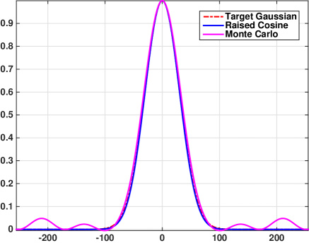
Fig. 1: Approximation of the range kernel $\psi(t)=\exp(-\alpha^{2}t^{2}/2)$ over the dynamic range $[-255,255]$, where $\alpha=1/30$. The raised cosine is of order $N=20$, and $T=200$ for the Monte Carlo approximation (obtained using a single realization of $X_{1}$).

2 Proposed Approximation

As a first step, we diagonalize the quadratic form in the definition of $\phi(\boldsymbol{x})$ using an orthogonal transform. Indeed, since $\mathbf{C}^{-1}$ is positive definite, we can find an orthogonal matrix $\mathbf{Q}\in\mathbb{R}^{d\times d}$ and positive numbers $\alpha_{1},\ldots,\alpha_{d}$ such that

$$\boldsymbol{x}^{T}\mathbf{C}^{-1}\boldsymbol{x}=\sum_{k=1}^{d}\alpha^{2}_{k}y_{k}^{2}\qquad\quad(\boldsymbol{y}=\mathbf{Q}^{T}\boldsymbol{x}),$$ (4)

where $\boldsymbol{y}=(y_{1},\ldots,y_{d})$. The change-of-basis $\boldsymbol{y}=\mathbf{Q}^{T}\boldsymbol{x}$ amounts to transforming the components of the vector-valued image at each pixel (similar to a color transformation). In particular, by defining the image $\boldsymbol{g}:\Omega\rightarrow\mathbb{R}^{d}$ given by

$$\boldsymbol{g}(\boldsymbol{i})=\mathbf{Q}^{T}\!\boldsymbol{f}(\boldsymbol{i}),$$

we can write (2) as

$$\mathcal{B}[\boldsymbol{f}](\boldsymbol{i})=\frac{1}{Z(\boldsymbol{i})}\sum_{\boldsymbol{j}}\omega(\boldsymbol{j})\ \psi\!\left(\boldsymbol{g}(\boldsymbol{i}-\boldsymbol{j})-\boldsymbol{g}(\boldsymbol{i})\right)\boldsymbol{f}(\boldsymbol{i}-\boldsymbol{j}),$$ (5)

where

$$Z(\boldsymbol{i})=\sum_{\boldsymbol{j}}\omega(\boldsymbol{j})\ \psi\!\left(\boldsymbol{g}(\boldsymbol{i}-\boldsymbol{j})-\boldsymbol{g}(\boldsymbol{i})\right).$$ (6)

Comparing (4) and the range kernel in (1), we see that $\psi:\mathbb{R}^{d}\rightarrow\mathbb{R}$ is given by

$$\psi(\boldsymbol{y})=\exp\!\left(-\frac{1}{2}\sum_{k=1}^{d}\alpha^{2}_{k}y_{k}^{2}\right)=\prod_{k=1}^{d}\exp\!\left(-\frac{1}{2}\alpha^{2}_{k}y_{k}^{2}\right).$$ (7)

The key point here is that we have factored the original kernel $\phi(\boldsymbol{x})$ into a product of one-dimensional Gaussians. At this point, we recall the following result from [7].

Proposition 2.1 (Raised-Cosine Approximation).

$$\lim_{N\rightarrow\infty}\ \left[\cos\!\left(\frac{\alpha t}{\sqrt{N}}\right)\right]^{N}\!=\exp\!\left(-\frac{1}{2}\alpha^{2}t^{2}\right).$$ (8)

We apply Proposition 2.1 to the one-dimensional Gaussians in (7), and conclude that

$$\psi(\boldsymbol{y})=\prod_{k=1}^{d}\lim_{N\rightarrow\infty}\left[\cos\!\left(\frac{\alpha_{k}y_{k}}{\sqrt{N}}\right)\right]^{N}\!\!\!=\lim_{N\rightarrow\infty}\prod_{k=1}^{d}\left[\cos\!\left(\frac{\alpha_{k}y_{k}}{\sqrt{N}}\right)\right]^{N}\!\!.$$

In practice, we fix some $N$, and replace (7) with

$$\psi(\boldsymbol{y})=\prod_{k=1}^{d}\left[\cos\!\left(\frac{\alpha_{k}y_{k}}{\sqrt{N}}\right)\right]^{N}.$$ (9)

To reduce unnecessary symbols, we have used $\psi(\boldsymbol{y})$ to represent both the original kernel and its approximation. This should not lead to a confusion, since we will not use the original kernel in the rest of the discussion. We will refer to $N$ as the order of the approximation.

The central observation of the paper is the following stochastic interpretation of (9), which is obtained by turning a product-of-sums into a sum-of-products.

Proposition 2.2.

Let $\mathbf{X}=(X_{1},\ldots,X_{d})$ be a random vector, whose components are independent and follow the binomial distribution $B(N,1/2)$. Then

$$\psi(\boldsymbol{y})=\mathbb{E}\left\{\prod_{k=1}^{d}\exp\!\big{(}\!\iota(N-2X_{k})\gamma_{k}y_{k}\big{)}\right\},$$ (10)

where $\iota=\sqrt{-1},\gamma_{k}=\alpha_{k}/\sqrt{N},$ and the expectation $\mathbb{E}[\cdot]$ is with respect to $\mathbf{X}$.

Proof.

Recall the identity $\cos\theta=(e^{\iota\theta}+e^{-\iota\theta})/2$, where $\iota=\sqrt{-1}$. We use this along with the binomial theorem, and get

$$\left(\cos\theta\right)^{N} =\frac{1}{2^{N}}\left(\exp(\iota\theta)+\exp(-\iota\theta)\right)^{N}$$

$$=\sum_{n=0}^{N}\frac{1}{2^{N}}\binom{N}{n}\exp\!\left(\iota(N-2n)\theta\right).$$ (11)

Notice that the coefficient in (2) corresponding to a given $n$ is simply the probability that a random variable $X\sim B(N,1/2)$ takes on the value $n$. In other words, we can write

$$\left(\cos\theta\right)^{N}=\mathbb{E}\Big{\{}\exp\!\left(\iota(N-2X)\theta\right)\Big{\}},$$ (12)

where $\mathbb{E}[\cdot]$ denotes the mathematical expectation with respect to $X$. Substituting (12) in (9), and using the independence assumption on the components of $\mathbf{X}$, we arrive at (10). ∎

(a) Dome ($876\times 584$).

(b) Direct, $75$ min.

(c) MCSF, $24$ sec.

Fig. 2: Results for the Dome image [3] at $\sigma_{s}=5$ and $\sigma_{r}=50$. The parameters for MCSF are $N=10$ and $T=200$. The MSE is $1.86$ dB.

We next approximate the mathematical expectation in (10) using Monte Carlo integration [12]. More specifically, let $F_{\mathbf{X}}$ denote the distribution of the random vector $\mathbf{X}$ in Proposition 2.2 that takes values in $\{0,1,\ldots,N\}^{d}$. We fix a certain number of trials $T$, and draw $\mathbf{X}^{(1)},\ldots,\mathbf{X}^{(T)}$ from $\{0,1,\ldots,N\}^{d}$ using the distribution $F_{\mathbf{X}}$. This gives us the following Monte Carlo approximation of (10):

$$\psi(\boldsymbol{y})=\frac{1}{T}\sum_{t=1}^{T}\left\{\prod_{k=1}^{d}\exp\!\big{(}\!\iota(N-2X^{(t)}_{k})\gamma_{k}y_{k}\big{)}\right\},$$ (13)

where $X^{(t)}_{k}$ is the $k$-th component of $\mathbf{X}^{(t)}$. To reduce symbols, we have again overloaded the notation for the original kernel in (7).

In summary, starting from the kernel in (7), we arrive at the approximation in (13) in two steps. First, we approximate the one-dimensional Gaussian using a raised-cosine of fixed order $N$. This results in a product of raised-cosines, which we express as a large sum-of-products. In the second step, we approximate the large sum using Monte Carlo integration. A comparison of the raised-cosine and the Monte Carlo approximations for a one-dimensional ($d=1$) range kernel is provided in Figure 1.

Before proceeding further, we simplify the expression in (13) by defining the random variable $\mathbf{Y}=(Y_{1},\ldots,Y_{d})$ given by

$$Y_{k}=N-2X_{k}\qquad\ (k=1,\ldots,d).$$

In terms of the realizations $\mathbf{Y}^{(1)},\ldots,\mathbf{Y}^{(T)}$, we can write (13) as

$$\psi(\boldsymbol{y})=\frac{1}{T}\sum_{t=1}^{T}\left\{\prod_{k=1}^{d}\exp\!\big{(}\iota Y^{(t)}_{k}\gamma_{k}y_{k}\big{)}\right\}.$$ (14)

3 Fast Algorithm

We now present the fast algorithm obtained by using (14) in place of the original Gaussian kernel. The fast algorithm is based on the so-called shiftability property of a function [11]. The shiftability of the exponential function follows from a rather simple fact, namely that $\exp(a+b)=\exp(a)\exp(b)$. In particular, on substituting (14) in (5), we can express the term $\psi\!\left(\boldsymbol{g}(\boldsymbol{i}-\boldsymbol{j})-\boldsymbol{g}(\boldsymbol{i})\right)$ as follows:

$$\frac{1}{T}\sum_{t=1}^{T}\Big{\{}\!\prod_{k=1}^{d}\exp\!\big{(}\!-\iota Y^{(t)}_{k}\gamma_{k}g_{k}(\boldsymbol{i})\big{)}\exp\!\big{(}\iota Y^{(t)}_{k}\gamma_{k}g_{k}(\boldsymbol{i}-\boldsymbol{j})\big{)}\Big{\}}$$ (15)

where $g_{k}(\boldsymbol{i})$ denotes the $k$-th component of $\boldsymbol{g}(\boldsymbol{i})$. We can simplify (15) by introducing the (complex-valued) image $h_{k,t}:\Omega\rightarrow\mathbb{C}$ given by

$$h_{k,t}(\boldsymbol{i})=\exp(\iota Y^{(t)}_{k}\gamma_{k}g_{k}(\boldsymbol{i})),$$

and the image $H_{t}:\Omega\rightarrow\mathbb{C}$ given by

$$H_{t}(\boldsymbol{i})=\prod_{k=1}^{d}h_{k,t}(\boldsymbol{i}).$$ (16)

In term of (16), note that we can write (15) as

$$\frac{1}{T}\sum_{t=1}^{T}H_{t}(\boldsymbol{i})^{\star}H_{t}(\boldsymbol{i}-\boldsymbol{j}),$$ (17)

where $H_{t}(\boldsymbol{i})^{\star}$ denotes the complex-conjugate of $H_{t}(\boldsymbol{i})$. Substituting (17) in (5), and exchanging the two sums, we obtain

$$\sum_{\boldsymbol{j}}\omega(\boldsymbol{j})\ \psi\!\left(\boldsymbol{g}(\boldsymbol{i}-\boldsymbol{j})-\boldsymbol{g}(i)\right)\boldsymbol{f}(\boldsymbol{i}-\boldsymbol{j})$$

$$=\frac{1}{T}\sum_{\boldsymbol{j}}\omega(\boldsymbol{j})\Big{\{}\sum_{t=1}^{T}H_{t}(\boldsymbol{i})^{\star}H_{t}(\boldsymbol{i}-\boldsymbol{j})\Big{\}}\boldsymbol{f}(\boldsymbol{i}-\boldsymbol{j})$$

$$=\frac{1}{T}\sum_{t=1}^{T}H_{t}(\boldsymbol{i})^{\star}\Big{\{}\sum_{\boldsymbol{j}}\omega(\boldsymbol{j})\mathbf{G}_{t}(\boldsymbol{i}-\boldsymbol{j})\Big{\}},$$ (18)

where the vector-valued image $\mathbf{G}_{t}:\Omega\rightarrow\mathbb{C}^{d}$ is given by $\mathbf{G}_{t}(\boldsymbol{i})=H_{t}(\boldsymbol{i})\boldsymbol{f}(\boldsymbol{i})$. Similarly, on substituting (14) in (6), we obtain

$$Z(\boldsymbol{i})=\frac{1}{T}\sum_{t=1}^{T}H_{t}(\boldsymbol{i})^{\star}\Big{\{}\sum_{\boldsymbol{j}}\omega(\boldsymbol{j})H_{t}(\boldsymbol{i}-\boldsymbol{j})\Big{\}}.$$ (19)

Notice that we have managed to express (5) and (6) using a series of Gaussian convolutions. Indeed, the term within brackets in (19) is a Gaussian convolution, which we denote by $\omega\ast H_{t}$. On the other hand, the Gaussian convolution in (3) is performed on each of the $d$ components of $\mathbf{G}_{t}$; we denote this using $\omega\ast{\mathbf{G}}_{t}$. Thus, we are required to perform a total of $T(d+1)$ Gaussian convolutions, which constitutes the bulk of the computation. The procedure for computing the proposed approximation of (2) is summarized in Algorithm 1. We shall henceforth refer to the proposed algorithm as the MCSF (Monte Carlo Shiftable Filter). Note that we can efficiently compute the Gaussian convolutions in step 1 using separability and recursion, and importantly, at $O(1)$ cost with respect to $\sigma_{s}$ [13]. The run-time of the proposed algorithm is thus independent of $\sigma_{s}$, and is hence expected to be much faster than the direct implementation for large $\sigma_{s}$. Needless to mention, we can replace the spatial filter $\omega(\boldsymbol{i})$ in (1) with any arbitrary spatial filter (such as a box or hat filter), and the above reductions would still hold.

Data: Image $\boldsymbol{f}:\Omega\rightarrow\mathbb{R}^{d}$, and parameters $\sigma_{s},\mathbf{C},N$, and $T$.

Result: Shiftable approximation of (2) denoted by $\mathcal{S}[\boldsymbol{f}]$.

1 Diagonalize $\mathbf{C}$ to get $\mathbf{Q}$ and $\alpha_{1},\ldots,\alpha_{d}$;

2 Set up the spatial filter $\omega(\boldsymbol{i})$ in (1) using $\sigma_{s}$;

3 for $k=1,2,3$ do

4       $\gamma_{k}=\alpha_{k}/\sqrt{N}$;

5      

6 end for

7for $\boldsymbol{i}\in\Omega$ do

8       Set $\boldsymbol{g}(\boldsymbol{i})=\mathbf{Q}^{T}\!\boldsymbol{f}(\boldsymbol{i})$;

9       Set $\mathbf{P}(\boldsymbol{i})=\mathbf{0}$;

10       Set $Z(\boldsymbol{i})=0$;

11      

12 end for

13for $t=1,\ldots,T$ do

14       Draw $\mathbf{X}$ from $B(N,1/2)^{d}$;

15       Set $H(\boldsymbol{i})=1$ for $\boldsymbol{i}\in\Omega$;

16       for $k=1,\ldots,d$ do

17             $H(\boldsymbol{i})=H(\boldsymbol{i})\exp\!\big{(}\iota(N-2X_{k})\gamma_{k}g_{k}(\boldsymbol{i})\big{)}$;

18            

19       end for

20      Set $\mathbf{G}(\boldsymbol{i})=H(\boldsymbol{i})\boldsymbol{f}(\boldsymbol{i})$ for $\boldsymbol{i}\in\Omega$;

21       Compute $\bar{\mathbf{G}}=\omega\ast\mathbf{G}$ and $\bar{H}=\omega\ast H$;

22       Set $\mathbf{P}(\boldsymbol{i})=\mathbf{P}(\boldsymbol{i})+H(\boldsymbol{i})^{\star}\bar{\mathbf{G}}(\boldsymbol{i})$ for $\boldsymbol{i}\in\Omega$;

23       Set $Z(\boldsymbol{i})=Z(\boldsymbol{i})+H(\boldsymbol{i})^{\star}\bar{H}(\boldsymbol{i})$ for $\boldsymbol{i}\in\Omega$;

24      

25 end for

Set $\mathcal{S}[\boldsymbol{f}](\boldsymbol{i})=Z[\boldsymbol{i}]^{-1}\mathbf{P}(\boldsymbol{i})$ for $\boldsymbol{i}\in\Omega$.

Algorithm 1 Monte Carlo Shiftable Filter (MCSF).

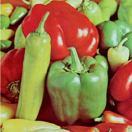
(a) Peppers [14].

(b) Direct, $38$ min.

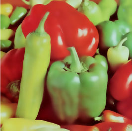
(c) MCSF, $16$ sec.

Fig. 3: Results for the $512\times 512$ Peppers image at $\sigma_{s}=5$ and $\sigma_{r}=80$. Parameters for MCSF are $N=10$ and $T=300$. The run-times are given in the caption. The MSE between (b) and (c) is $0.34$ dB.

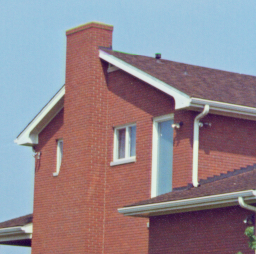
(a) House [14].

(b) Direct, $8.5$ min.

(c) MCSF, $5$ sec.

Fig. 4: Results for the $256\times 256$ House image at $\sigma_{s}=5$ and $\sigma_{r}=90$. The parameters for MCSF are $N=10$ and $T=300$. The MSE between (b) and (c) is $-1.48$ dB.

4 Results for Color Images

In this section, we present some results on natural color images for which $d=3$. In particular, we demonstrate that the proposed MCSF algorithm is both fast and accurate for color images in relation to the direct implementation. To quantify the approximation accuracy for a given color image $\boldsymbol{f}:\Omega\rightarrow\mathbb{R}^{3}$, we used the mean-squared error between $\mathcal{B}[\boldsymbol{f}]$ and $\mathcal{S}[\boldsymbol{f}]$ (the latter is the output of Algorithm 1) given by

$$\text{MSE}=\frac{1}{3|\Omega|}\sum_{k=1}^{3}\sum_{\boldsymbol{i}\in\Omega}\big{(}\mathcal{B}[\boldsymbol{f}]_{k}(\boldsymbol{i})-\mathcal{S}[\boldsymbol{f}]_{k}(\boldsymbol{i})\big{)}^{2},$$ (20)

where $\mathcal{B}[\boldsymbol{f}]_{k}$ and $\mathcal{S}[\boldsymbol{f}]_{k}$ are the $k$-th color channel. On a logarithmic scale, this corresponds to $10\log_{10}(\text{MSE})$ dB. For the experiments reported in this paper, we used an isotropic Gaussian kernel corresponding to $\mathbf{C}=\sigma_{r}^{2}\mathbf{I}$ in (1). In other words, $\mathbf{Q}=\mathbf{I}$, and $\alpha_{k}=1/\sigma_{r}$ for $k=1,2,3$.

The accuracy of the proposed algorithm is controlled by the order of the raised-cosine ($N$) and the number of trails ($T$). It is clear that we can improve the approximation accuracy by increasing $N$ and $T$. We illustrate this point with an example in Figure 5. We notice that MCSF can achieve sub-pixel accuracy when $N=10$ and $T>300$. We have noticed in our simulations that, for a fixed $T$, the accuracy tends to saturate beyond a certain $N$. This is demonstrated in Figure 5 using $N=10$ and $N=20$.

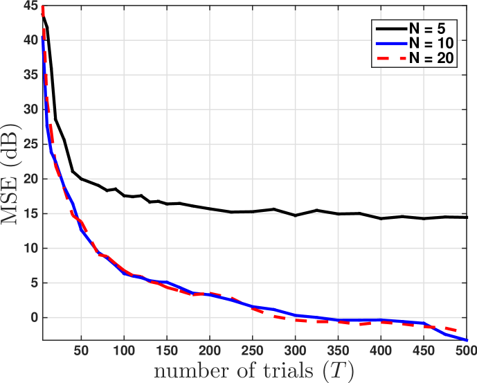
Fig. 5: Plot of the MSE given by (20) as a function of the number of Monte Carlo trails. The Dome image [3] was used for this experiment, and the parameters are $\sigma_{s}=1$ and $\sigma_{r}=30$. For a fixed $N$ and $T$, the MSE was averaged over $400$ Monte Carlo realizations.

Table 1: Comparison of the run-time of the direct implementation and Algorithm 1 on the $512\times 512$ Peppers image. The range parameter used is $\sigma_{r}=40$. The parameters of MCSF are $N=10$ and $T=300$. The computations were performed using Matlab $8.4$ on a $3.40$ GHz Intel $4$-core machine with $32$ GB memory.

Method $\backslash$ $\sigma_{s}$	$1$	$2$	$3$	$4$	$5$	$10$
Direct	116s	6.6m	14.6m	24.1m	36.5m	141m
MCSF	16.9s	17.1s	17.2s	17.3s	17.3s	17.5s

A comparison of the run-time of the direct implementation of (2) and that of the proposed algorithm is provided in Table 1. We notice that MCSF is few orders faster than the direct implementation, particularly for large $\sigma_{s}$. Indeed, following the fact that the convolutions in step 1 of Algorithm 1 can be computed in constant-time with respect to $\sigma_{s}$ [13], our algorithm has $O(1)$ complexity with respect to $\sigma_{s}$. As against this, the direct implementation scales as $O(\sigma_{s}^{2})$.

Finally, we present a visual comparison of the filtering for RGB images in Figures 2 and 3. Notice that the outputs are visually indistinguishable. As mentioned earlier, the authors in [1, 3] have observed that the application of the bilateral filter in the RGB color space can lead to color leakage, particularly at the sharp edges. The suggested solution was to perform the filtering in the CIE-Lab space [15]. In this regard, a comparison of the filtering in the CIE-Lab space is provided in Figure 4. In this case, we first performed a color transformation from the RGB to the CIE-Lab space, performed the filtering in the CIE-Lab space, and then transformed back to the RGB space. The filtered outputs are seen to be close, both visually and in terms of the MSE.

5 Conclusion

We proposed a fast algorithm for the bilateral filtering of vector-valued images. We applied the algorithm for filtering color images in the RGB and the CIE-Lab space. In particular, we demonstrated that a speedup of few orders can be achieved using the fast algorithm without introducing visible changes in the filter output (the latter fact was also quantified using the MSE). An important theoretical question arising from the work is the dependence of the order and the number of trials on the filtering accuracy. In future work, we will investigate this matter, and also look at various ways of improving the Monte Carlo integration [12]. We also plan to test the algorithm on other vector-valued images.

References

• [1] C. Tomasi and R. Manduchi, “Bilateral filtering for gray and color images,” Proc. IEEE International Conference on Computer Vision, pp. 839-846, 1998.
• [2] P. Kornprobst and J. Tumblin, Bilateral Filtering: Theory and Applications. Now Publishers Inc., 2009.
• [3] S. Paris and F. Durand, “A fast approximation of the bilateral filter using a signal processing approach,” International Journal of Computer Vision, vol. 81, no. 1, pp. 25-52, 2009.
• [4] B. Weiss, “Fast median and bilateral filtering,” Proc. ACM Siggraph, vol. 25, pp. 519-526, 2006.
• [5] F. Porikli, “Constant time $O(1)$ bilateral filtering,” Proc. IEEE Conference on Computer Vision and Pattern Recognition, pp. 1-8, 2008.
• [6] Q. Yang, K. H. Tan, and N. Ahuja, “Real-time $O(1)$ bilateral filtering,” Proc. IEEE Conference on Computer Vision and Pattern Recognition, pp. 557-564, 2009.
• [7] K. N. Chaudhury, D. Sage, and M. Unser, “Fast $O(1)$ bilateral filtering using trigonometric range kernels,” IEEE Transactions on Image Processing, vol. 20, no. 12, pp. 3376-3382, 2011.
• [8] K. Sugimoto and S. I. Kamata, “Compressive bilateral filtering,” IEEE Transactions on Image Processing, vol. 24, no. 11, pp. 3357-3369, 2015.
• [9] K. N. Chaudhury and S. Dabhade, “Fast and provably accurate bilateral filtering,” vol. 25, no. 6, pp. 2519-2528, IEEE Transactions on Image Processing, 2016.
• [10] K. N. Chaudhury, “Constant-time filtering using shiftable kernels,” IEEE Signal Processing Letters, vol. 18, no. 11, pp. 651-654, 2011.
• [11] K. N. Chaudhury, “Acceleration of the shiftable algorithm for bilateral filtering and nonlocal means,” IEEE Transactions on Image Processing, vol. 22, no. 4, pp. 1291-1300, 2013.
• [12] A. Doucet and X. Wang, “Monte Carlo methods for signal processing: a review in the statistical signal processing context,” IEEE Signal Processing Magazine, vol. 22, no. 6, pp. 152-170, 2005.
• [13] R. Deriche, “Recursively implementing the Gaussian and its derivatives,” Research Report, INRIA-00074778, 1993.
• [14] BM3D Image Database, http://www.cs.tut.fi/foi/GCF-BM3D.
• [15] G. Wyszecki and W. S. Styles, Color Science. Wiley, New York, 1982.