EUROPEAN ORGANIZATION FOR NUCLEAR RESEARCH (CERN)

​​​ CERN-EP-2016-083 LHCb-PAPER-2016-006 28 June 2016

Model-independent measurement of the CKM angle $\gamma$ using $B^{0}\rightarrow D{{K}^{*0}}$ decays with $D\rightarrow{{K}^{0}_{\mathrm{\scriptscriptstyle S}}}{{\pi}^{+}}{{\pi}^{-}}$ and ${{K}^{0}_{\mathrm{\scriptscriptstyle S}}}{{K}^{+}}{{K}^{-}}$

The LHCb collaboration

A binned Dalitz plot analysis of the decays ${{B}^{0}}\rightarrow D{{K}^{*0}}$, with $D\rightarrow{{K}^{0}_{\mathrm{\scriptscriptstyle S}}}{{\pi}^{+}}{{\pi}^{-}}$ and $D\rightarrow{{K}^{0}_{\mathrm{\scriptscriptstyle S}}}{{K}^{+}}{{K}^{-}}$, is performed to measure the observables $x_{\pm}$ and $y_{\pm}$, which are related to the CKM angle $\gamma$ and the hadronic parameters of the decays. The $D$ decay strong phase variation over the Dalitz plot is taken from measurements performed at the CLEO-c experiment, making the analysis independent of the $D$ decay model. With a sample of proton-proton collision data, corresponding to an integrated luminosity of 3.0 $\mbox{\,fb}^{-1}$, collected by the LHCb experiment, the values of the $C\!P$ violation parameters are found to be $x_{+}=0.05\pm 0.35\pm 0.02$, $x_{-}=-0.31\pm 0.20\pm 0.04$, $y_{+}=-0.81\pm 0.28\pm 0.06$ and $y_{-}=0.31\pm 0.21\pm 0.05$, where the first uncertainties are statistical and the second systematic. These observables correspond to values $\gamma$ = $(71\pm 20)^{\circ}$, $r_{B^{0}}=0.56\pm 0.17$ and $\delta_{B^{0}}=(204\,^{+21}_{-20})^{\circ}$. The parameters $r_{B^{0}}$ and $\delta_{B^{0}}$ are the magnitude ratio and strong phase difference between the suppressed and favoured $B^{0}$ decay amplitudes, and have been measured in a region of $\pm 50{\mathrm{\,Me\kern-1.00006ptV\!/}c^{2}}$ around the ${{K}^{*}}(892)^{0}$ mass and with the magnitude of the cosine of the ${{K}^{*}}(892)^{0}$ helicity angle larger than 0.4.

Published in JHEP 06 (2016) 131

© CERN on behalf of the LHCb collaboration, licence CC-BY-4.0.

 

1 Introduction

The Standard Model (SM) description of $C\!P$ violation can be tested through measurements of the angle $\gamma$ of the unitarity triangle of the Cabibbo-Kobayashi-Maskawa (CKM) matrix [1, 2], where $\gamma\equiv\mathrm{arg}(-V_{ud}^{\phantom{\ast}}V_{ub}^{\ast}/V_{cd}^{\phantom{\ast}}V_{cb}^{\ast})$. It is the only CKM angle easily accessible in tree-level processes and can be measured, with a small uncertainty from theory of $\delta\gamma/\gamma\leq 10^{-7}$ [3]. Hence, in the absence of new physics effects at tree level [4], a precision measurement of $\gamma$ provides an SM benchmark which can be compared with other CKM matrix observables that are more likely to be affected by physics beyond the SM. Such comparisons are currently limited by the uncertainty on direct measurements of $\gamma$, which is about $7^{\circ}$ [5, 6].

The CKM angle $\gamma$ is experimentally accessible through the interference between $\bar{b}\rightarrow\bar{c}u\bar{s}$ and $\bar{b}\rightarrow\bar{u}c\bar{s}$ transitions. The traditional golden mode is ${{{B}^{-}}}\rightarrow{D}{{K}^{-}}$, with charge-conjugation implied throughout, where $D$ represents a neutral $D$ meson reconstructed in a final state that is common to both ${D}^{0}$ and ${\kern 1.99997pt\overline{\kern-1.99997ptD}{}}{}^{0}$ decays. This mode has been studied at LHCb with a wide range of $D$ meson final states to measure observables with sensitivity to $\gamma$ [7, 8, 9, 10]. In addition to these studies, other $B$ decays have also been used with a variety of techniques to determine $\gamma$ [11, 12, 13, 14].

This paper presents an analysis in which the decay ${{B}^{0}}\rightarrow D{{K}^{*0}}$ provides sensitivity to the CKM angle $\gamma$ through the interfering amplitudes shown in Fig. 1. Here the ${K}^{*0}$ refers to the ${{K}^{*}}(892)^{0}$, and the charge of the kaon from the ${K}^{*0}$ unambiguously identifies the flavour of the decaying $B$ meson as ${B}^{0}$ or ${\kern 1.79993pt\overline{\kern-1.79993ptB}{}}{}^{0}$. Although the branching fraction of the ${{B}^{0}}\rightarrow D{{K}^{*0}}$ decay is an order of magnitude smaller than that of the ${{{B}^{-}}}\rightarrow D{{K}^{-}}$ decay [15], it is expected to exhibit larger $C\!P$-violating effects as the two colour-suppressed Feynman diagrams in Fig. 1 are comparable in magnitude. Measurements sensitive to $\gamma$ using the ${{B}^{0}}\rightarrow D{{K}^{*0}}$ decay mode were pioneered by the BaBar [16] and Belle [17] collaborations, and have been pursued by the LHCb collaboration [11, 14].

Figure 1: Feynman diagrams of the (left) ${{B}^{0}}\rightarrow{{D}^{0}}{{K}^{*0}}$ and (right) ${{B}^{0}}\rightarrow{{\kern 1.99997pt\overline{\kern-1.99997ptD}{}}{}^{0}}{{K}^{*0}}$ amplitudes, which interfere in the ${{B}^{0}}\rightarrow D{{K}^{*0}}$ decay.

The three-body self-conjugate decays $D\rightarrow{{K}^{0}_{\mathrm{\scriptscriptstyle S}}}{{\pi}^{+}}{{\pi}^{-}}$ and $D\rightarrow{{K}^{0}_{\mathrm{\scriptscriptstyle S}}}{{K}^{+}}{{K}^{-}}$, designated collectively as $D\rightarrow{{K}^{0}_{\mathrm{\scriptscriptstyle S}}}h^{+}h^{-}$, are accessible to both ${D}^{0}$ and ${\kern 1.99997pt\overline{\kern-1.99997ptD}{}}{}^{0}$. They have large variation of the strong phase over the Dalitz plot, and thus provide a powerful method to determine the angle $\gamma$. Sensitivity to $\gamma$ is obtained by comparing the distribution of events in the $D\rightarrow{{K}^{0}_{\mathrm{\scriptscriptstyle S}}}h^{+}h^{-}$ Dalitz plots of $B$ mesons reconstructed in each flavour, as described in Refs. [18, 19, 20]. To determine $\gamma$ from the comparison, input is required on the variation within the Dalitz plot of the strong-interaction phase difference between ${D}^{0}$ and ${\kern 1.99997pt\overline{\kern-1.99997ptD}{}}{}^{0}$ decays. An amplitude model of the ${{D}^{0}}\rightarrow{{K}^{0}_{\mathrm{\scriptscriptstyle S}}}h^{+}h^{-}$ decay can be used to provide this information and this technique has been used to study the ${{B}^{0}}\rightarrow D{{K}^{*0}}$, $D\rightarrow{{K}^{0}_{\mathrm{\scriptscriptstyle S}}}{{\pi}^{+}}{{\pi}^{-}}$ decay mode by BaBar [21] and LHCb [22]. In Ref. [22] the same dataset is used as the one analysed in this paper. An attractive alternative is to use model-independent measurements of the strong-phase difference variation over the Dalitz plot, which removes the need to assign model-related systematic uncertainties [19, 20]. Measurements of the strong-phase variation in binned regions of the Dalitz plot cannot be done with LHCb data alone, but can be accomplished using an analysis of quantum-correlated neutral $D$ meson pairs from $\psi(3770)$ decays, and have been made at the CLEO-c experiment [23]. These measurements have direct access to the strong-phase difference, which is not the case for the amplitude models based on fits to flavour-tagged $D$ decays only [24, 25]. The separation of data into binned regions of the Dalitz plot leads to a loss in statistical sensitivity in comparison to using an amplitude model; however, the advantage of using the measurements from CLEO is that the systematic uncertainties remain free of any model assumptions on the strong-phase difference. This model-independent method has been used by Belle [26] to study the ${{B}^{0}}\rightarrow D{{K}^{*0}}$, $D\rightarrow{{K}^{0}_{\mathrm{\scriptscriptstyle S}}}{{\pi}^{+}}{{\pi}^{-}}$ decay mode, and by LHCb [8] and Belle [27] to study ${{B}^{\pm}}\rightarrow D{{K}^{\pm}}$ decays.

In this paper, $pp$ collision data at a centre-of-mass energy $\sqrt{s}=7\,(8)\mathrm{\,Te\kern-1.00006ptV}$, accumulated by LHCb in 2011 (2012) and corresponding to a total integrated luminosity of $3.0\mbox{\,fb}^{-1}$, are exploited to perform a model-independent measurement of $\gamma$ in the decay mode ${{B}^{0}}\rightarrow D{{K}^{*0}}$, with $D\rightarrow{{K}^{0}_{\mathrm{\scriptscriptstyle S}}}{{\pi}^{+}}{{\pi}^{-}}$ and $D\rightarrow{{K}^{0}_{\mathrm{\scriptscriptstyle S}}}{{K}^{+}}{{K}^{-}}$. The yield of ${{B}^{0}}\rightarrow D{{K}^{*0}}$ with $D\rightarrow{{K}^{0}_{\mathrm{\scriptscriptstyle S}}}{{\pi}^{+}}{{\pi}^{-}}$ is twice that previously analysed at Belle [27] and the $D\rightarrow{{K}^{0}_{\mathrm{\scriptscriptstyle S}}}{{K}^{+}}{{K}^{-}}$ decay is included for the first time. This allows for a precise measurement of $x_{\pm},y_{\pm}$ using the techniques developed for similar analyses of ${{{B}^{-}}}\rightarrow{D}{{K}^{-}}$ decays [8].

The remainder of the paper is organised as follows. Section 2 describes the analysis framework. Section 3 describes the LHCb detector, and Sect. 4 presents the candidate selection and the parametrisation of the $B$ candidate invariant mass spectrum. Section 5 is concerned with the use of semileptonic decays in order to determine the populations in different bins of the ${{D}^{0}}\rightarrow{{K}^{0}_{\mathrm{\scriptscriptstyle S}}}h^{+}h^{-}$ Dalitz plot. Section 6 discusses the binned Dalitz plot fit and presents the measurements of the $C\!P$ violation parameters. The evaluation of systematic uncertainties is summarised in Sect. 7. The determination of the CKM angle $\gamma$ using the measured $C\!P$ parameters is described in Sect. 8.

2 Overview of the analysis

The favoured and suppressed ${B}^{0}$ decay amplitudes can be expressed as

$$A({{B}^{0}}\rightarrow{{\kern 1.99997pt\overline{\kern-1.99997ptD}{}}{}^{0}}X^{0}_{s};p) \equiv A_{c}(p)e^{i\delta_{c}(p)},$$ (1)

$$A({{B}^{0}}\rightarrow{{D}^{0}}X^{0}_{s};p) \equiv A_{u}(p)e^{i[\delta_{u}(p)+\gamma]},$$

where $p$ is the $\left(m^{2}(K\pi),m^{2}(D\pi)\right)$ coordinate on the ${{B}^{0}}\rightarrow{D}K\pi$ Dalitz plot, $A_{u}(p)$ and $A_{c}(p)$ are the moduli of the $b\rightarrow u$ and $b\rightarrow c$ amplitudes, and $\delta_{c,u}(p)$ represent the strong phases of the relevant decay amplitudes. The symbol $X^{0}_{s}$ refers to a resonant or nonresonant ${{K}^{+}}{{\pi}^{-}}$ pair, which could be produced by the decay of the ${K}^{*0}$ meson or by other contributions to the ${{B}^{0}}\rightarrow{D}{{K}^{+}}{{\pi}^{-}}$ final state. Similar expressions can be written for the ${\kern 1.79993pt\overline{\kern-1.79993ptB}{}}{}^{0}$ decay, where the parameter $\gamma$ enters with opposite sign. The natural width of the ${K}^{*0}$ (approximately $50{\mathrm{\,Me\kern-1.00006ptV\!/}c^{2}}$ [15]) must be considered when analysing these decays. In the region near the ${K}^{*0}$ mass there is interference between the signal ${K}^{*0}$ decay amplitude and amplitudes due to the other ${{B}^{0}}\rightarrow D{{K}^{+}}{{\pi}^{-}}$ Dalitz plot contributions, such as higher mass $K\pi$ resonances and nonresonant $K\pi$ decays. Hence, the magnitude ratio between the suppressed and favoured amplitudes $r_{{{B}^{0}}}$, the coherence factor $\kappa$ [28], and the effective strong phase difference $\delta_{{{B}^{0}}}$ depend on the region of the ${B}^{0}$ Dalitz plot to be analysed. These are defined as

$$r^{2}_{{{B}^{0}}} \equiv\frac{|A({{B}^{0}}\rightarrow{{D}^{0}}{{K}^{*0}})|^{2}}{|A({{B}^{0}}\rightarrow{{\kern 1.99997pt\overline{\kern-1.99997ptD}{}}{}^{0}}{{K}^{*0}})|^{2}}=\frac{\int_{{K}^{*0}}dp\,A_{u}^{2}(p)}{\int_{{{K}^{*0}}}dp\,A_{c}^{2}(p)},$$ (2)

$$\kappa e^{i\delta_{{{B}^{0}}}} \equiv\frac{\int_{{K}^{*0}}dp\,A_{c}(p)A_{u}(p)e^{i[\delta_{u}(p)-\delta_{c}(p)]}}{\sqrt{\int_{{K}^{*0}}dp\,A_{c}^{2}(p)}\sqrt{\int_{{K}^{*0}}dp\,A_{u}^{2}(p)}},$$ (3)

where $0\leq\kappa\leq 1$. For this analysis the integration is over $K^{+}\pi^{-}$ masses within $50{\mathrm{\,Me\kern-1.00006ptV\!/}c^{2}}$ of the known ${K}^{*0}$ mass [15] and an absolute value of the cosine of the ${K}^{*0}$ helicity angle $\theta^{\ast}$ greater than 0.4. The helicity angle $\theta^{\ast}$ is defined as the angle between the ${K}^{*0}$ daughter kaon momentum vector and the direction opposite to the ${B}^{0}$ momentum vector in the ${K}^{*0}$ rest frame. This region is chosen to obtain a large value of $\kappa$ and to facilitate combination with results in Refs. [11, 14], which impose the same limits. The coherence factor has recently been determined by the LHCb collaboration to be $\kappa=0.958\,^{+0.005}_{-0.010}\,{}^{+0.002}_{-0.045}$ [14], through an amplitude analysis that measures the $b\rightarrow c$ and $b\rightarrow u$ amplitudes in the ${{B}^{0}}\rightarrow DK^{+}\pi^{-}$ decay.

The amplitude of the ${D}^{0}$ meson decay at a particular point on the $D$ Dalitz plot is defined as $A_{D}(m^{2}_{-},m^{2}_{+})\equiv A(m^{2}_{-},m^{2}_{+})e^{i\delta(m^{2}_{-},m^{2}_{+})}$, where $m^{2}_{-}$ ($m^{2}_{+}$) is the invariant mass of the ${{K}^{0}_{\mathrm{\scriptscriptstyle S}}}h^{-}$ (${{K}^{0}_{\mathrm{\scriptscriptstyle S}}}h^{+}$) pair. Neglecting $C\!P$ violation in charm decays, which is known to be small [15], the charge-conjugated amplitudes are related by $A_{\overline{D}}(m^{2}_{-},m^{2}_{+})=A_{D}(m^{2}_{+},m^{2}_{-})$. The partial widths for the $B$ decays can be written as

$$d{\Gamma}({{\kern 1.79993pt\overline{\kern-1.79993ptB}{}}{}^{0}}\rightarrow D(\rightarrow{{K}^{0}_{\mathrm{\scriptscriptstyle S}}}h^{+}h^{-}) \overline{X}^{0}_{s};p,m^{2}_{-},m^{2}_{+})\propto$$ (4)

$$\bigl{\lvert}A_{c}(p)e^{i\delta_{c}(p)}A_{D}(m^{2}_{-},m^{2}_{+})+A_{u}(p)e^{i[\delta_{u}(p)-\gamma]}A_{\overline{D}}(m^{2}_{-},m^{2}_{+})\bigr{\rvert}^{2},$$

$$d{\Gamma}({{B}^{0}}\rightarrow D(\rightarrow{{K}^{0}_{\mathrm{\scriptscriptstyle S}}}h^{+}h^{-}) {X^{0}_{s}};p,m^{2}_{-},m^{2}_{+})\propto$$ (5)

$$\bigl{\lvert}A_{c}(p)e^{i\delta_{c}(p)}A_{\overline{D}}(m^{2}_{-},m^{2}_{+})+A_{u}(p)e^{i[\delta_{u}(p)+\gamma]}A_{D}(m^{2}_{-},m^{2}_{+})\bigr{\rvert}^{2}.$$

Expanding and integrating over the defined ${K}^{*0}$ region, one obtains

$$d{\Gamma} ({{\kern 1.79993pt\overline{\kern-1.79993ptB}{}}{}^{0}}\rightarrow D(\rightarrow{{K}^{0}_{\mathrm{\scriptscriptstyle S}}}h^{+}h^{-}){{\kern 1.99997pt\overline{\kern-1.99997ptK}{}}{}^{*0}};m^{2}_{-},m^{2}_{+})\propto$$ (6)

$$\bigl{\lvert}A_{D}(m^{2}_{-},m^{2}_{+})\bigr{\rvert}^{2}+r_{{{B}^{0}}}^{2}\bigl{\lvert}A_{D}(m^{2}_{+},m^{2}_{-})\bigr{\rvert}^{2}+2\kappa r_{{{B}^{0}}}\mathrm{Re}\big{[}A_{D}(m^{2}_{-},m^{2}_{+})A^{*}_{D}(m^{2}_{+},m^{2}_{-})e^{-i(\delta_{{{B}^{0}}}-\gamma)}\big{]},$$

$$d{\Gamma} ({{B}^{0}}\rightarrow D(\rightarrow{{K}^{0}_{\mathrm{\scriptscriptstyle S}}}h^{+}h^{-}){{{K}^{*0}}};m^{2}_{-},m^{2}_{+})\propto$$ (7)

$$\bigl{\lvert}A_{D}(m^{2}_{+},m^{2}_{-})\bigr{\rvert}^{2}+r_{{{B}^{0}}}^{2}\bigl{\lvert}A_{D}(m^{2}_{-},m^{2}_{+})\bigr{\rvert}^{2}+2\kappa r_{{{B}^{0}}}\mathrm{Re}\big{[}A_{D}(m^{2}_{+},m^{2}_{-})A^{*}_{D}(m^{2}_{-},m^{2}_{+})e^{-i(\delta_{{{B}^{0}}}+\gamma)}\big{]}.$$

The $D$ Dalitz plot is partitioned into bins symmetric under the exchange $m^{2}_{-}\leftrightarrow m^{2}_{+}$. The cosine of the strong-phase difference between the ${D}^{0}$ and ${\kern 1.99997pt\overline{\kern-1.99997ptD}{}}{}^{0}$ decay weighted by the decay amplitude and averaged in bin $i$ is called $c_{i}$ [19, 20], and is given by

$$c_{i} \equiv\frac{\int_{i}dm^{2}_{-}\,dm^{2}_{+}\,A(m^{2}_{-},m^{2}_{+})A(m^{2}_{+},m^{2}_{-})\cos[\delta(m^{2}_{-},m^{2}_{+})-\delta(m^{2}_{+},m^{2}_{-})]}{\sqrt{\int_{i}dm^{2}_{-}\,dm^{2}_{+}\,A^{2}(m^{2}_{-},m^{2}_{+})\int_{i}dm^{2}_{-}\,dm^{2}_{+}\,A^{2}(m^{2}_{+},m^{2}_{-})}},$$ (8)

where the integrals are evaluated over the phase space of bin $i$. An analogous expression can be written for $s_{i}$ which is the sine of the strong-phase difference weighted by the decay amplitude and averaged in the bin.

Measurements of $c_{i}$ and $s_{i}$ are provided by CLEO in four different $2\times 8$ binning schemes for the $D\rightarrow{{K}^{0}_{\mathrm{\scriptscriptstyle S}}}{{\pi}^{+}}{{\pi}^{-}}$ decay [23]. The bins are labelled from $-8$ to $+8$, excluding zero, where the bins containing a positive label satisfy the condition $m^{2}_{-}\geq m^{2}_{+}$. The binning scheme used in this analysis is referred to as the ‘modified optimal’ binning. The optimisation was performed assuming a strong-phase difference distribution given by the BaBar model presented in Ref. [24]. This modified optimal binning is described in Ref. [23] and was designed to be statistically optimal in a scenario where the signal purity is low. It is also more robust for analyses with low yields in comparison to the alternatives, as no individual bin is very small. For the ${{K}^{0}_{\mathrm{\scriptscriptstyle S}}}{{K}^{+}}{{K}^{-}}$ final state, the measurements of $c_{i}$ and $s_{i}$ are available in three variants containing a different number of bins, with the guiding model being that from the BaBar study described in Ref. [25]. For the present analysis the variant with the $2\times 2$ binning is chosen, given the very low signal yields expected in this decay. The measurements of $c_{i}$ and $s_{i}$ are not biased by the use of a specific amplitude model in defining the bin boundaries, which only affects this analysis to the extent that if the model gives a poor description of the underlying decay then there will be a reduction in the statistical sensitivity of the $\gamma$ measurement. The binning choices for the two decay modes are shown in Fig. 2.

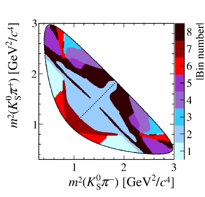
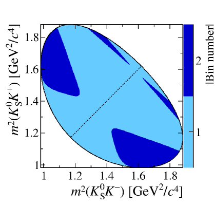
Figure 2: Binning schemes for (left) $D\rightarrow{{K}^{0}_{\mathrm{\scriptscriptstyle S}}}{{\pi}^{+}}{{\pi}^{-}}$ and (right) $D\rightarrow{{K}^{0}_{\mathrm{\scriptscriptstyle S}}}{{K}^{+}}{{K}^{-}}$. The diagonal line separates the positive and negative bin numbers, where the positive bins are in the region $m^{2}_{-}\geq m^{2}_{+}$.

The integrals of Eqs. (6) and (7) over the phase space of a Dalitz plot bin are proportional to the expected yield in that bin. The physics parameters of interest, $r_{{{B}^{0}}}$, $\delta_{{{B}^{0}}}$, and $\gamma$, are translated into four Cartesian variables [29, 30]. These are the measured observables and are defined as

$$x_{\pm}\equiv r_{{{B}^{0}}}\cos(\delta_{{{B}^{0}}}\pm\gamma)\;\mathrm{and}\;y_{\pm}\equiv r_{{{B}^{0}}}\sin(\delta_{{{B}^{0}}}\pm\gamma).$$ (9)

From Eqs. (6) and (7) it follows that

$$N_{\pm i}^{+} =n_{+}\left[F_{\mp i}+(x_{+}^{2}+y_{+}^{2})F_{\pm i}+2\kappa\sqrt{F_{+i}F_{-i}}(x_{+}c_{\pm i}-y_{+}s_{\pm i})\right],$$ (10)

$$N_{\pm i}^{-} =n_{-}\left[F_{\pm i}+(x_{-}^{2}+y_{-}^{2})F_{\mp i}+2\kappa\sqrt{F_{+i}F_{-i}}(x_{-}c_{\pm i}+y_{-}s_{\pm i})\right],$$ (11)

where $F_{i}$ are defined later in Eq. (12) and $N^{+}_{i}$ ($N^{-}_{i}$) is the expected number of ${B}^{0}$ (${\kern 1.79993pt\overline{\kern-1.79993ptB}{}}{}^{0}$) decays in bin $i$. The superscript on $N$ refers to the charge of the kaon from the ${K}^{*0}$ decay. The parameters $n_{+}$ and $n_{-}$ provide the normalisation, which can be different due to production, detection and $C\!P$ asymmetries between ${B}^{0}$ and ${\kern 1.79993pt\overline{\kern-1.79993ptB}{}}{}^{0}$ mesons. However the integrated yields are not used and the analysis is insensitive to such effects. The detector and selection requirements placed on the data lead to a non-uniform efficiency over the Dalitz plot. The efficiency profile for the signal candidates is given by $\eta=\eta(m^{2}_{-},m^{2}_{+})$. Only the relative efficiency from one point to another matters and not the absolute normalisation. The parameters $F_{i}$ are given by

$$F_{i}=\frac{\int_{i}dm^{2}_{-}dm^{2}_{+}|A_{D}(m^{2}_{-},m^{2}_{+})|^{2}\,\eta(m^{2}_{-},m^{2}_{+})}{\sum_{j}\int_{j}dm^{2}_{-}dm^{2}_{+}|A_{D}(m^{2}_{-},m^{2}_{+})|^{2}\,\eta(m^{2}_{-},m^{2}_{+})}$$ (12)

and are the fraction of decays in bin $i$ of the ${{D}^{0}}\rightarrow{{K}^{0}_{\mathrm{\scriptscriptstyle S}}}h^{+}h^{-}$ Dalitz plot.

The values of $F_{i}$ are determined from the control decay mode ${{B}^{0}}\rightarrow{{D}^{*-}}\mu^{+}\nu_{\mu}X$, where the ${D}^{*-}$ decays to ${\kern 1.99997pt\overline{\kern-1.99997ptD}{}}{}^{0}$ ${\pi}^{-}$ and the ${\kern 1.99997pt\overline{\kern-1.99997ptD}{}}{}^{0}$ decays to either the ${{K}^{0}_{\mathrm{\scriptscriptstyle S}}}{{\pi}^{+}}{{\pi}^{-}}$ or ${{K}^{0}_{\mathrm{\scriptscriptstyle S}}}{{K}^{+}}{{K}^{-}}$ final state. The symbol $X$, hereinafter omitted, indicates other particles which may be produced in the decay but are not reconstructed. Samples of simulated events are used to correct for the small differences in efficiency arising through necessary differences in selecting ${{B}^{0}}\rightarrow{{D}^{*-}}\mu^{+}\nu_{\mu}$ and ${{B}^{0}}\rightarrow D{{K}^{*0}}$ decays, which are discussed further in Sect. 5.

Effects due to ${D}^{0}$-${\kern 1.99997pt\overline{\kern-1.99997ptD}{}}{}^{0}$ mixing and $C\!P$ violation in ${K}^{0}$-${\kern 1.99997pt\overline{\kern-1.99997ptK}{}}{}^{0}$ mixing are ignored: the corrections are discussed in Refs. [31, 32] and are expected to be of order $0.2^{\circ}$ ($1^{\circ}$) for $D$ mixing ($C\!P$ violation in $K$ mixing) in ${{{B}^{-}}}\rightarrow D{{K}^{-}}$ decays. In both cases the size of the correction is reduced as the value of $r_{{{B}^{0}}}$ is expected to be approximately three times larger than the value of $r_{B}$ in ${{{B}^{-}}}\rightarrow D{{K}^{-}}$ decays. The effect of different nuclear interactions within the detector material for ${K}^{0}$ and ${\kern 1.99997pt\overline{\kern-1.99997ptK}{}}{}^{0}$ mesons is expected to be of a similar magnitude and is also ignored [33].

3 Detector and simulation

The LHCb detector [34, 35] is a single-arm forward spectrometer covering the pseudorapidity range $2<\eta<5$, designed for the study of particles containing $b$ or $c$ quarks. The detector includes a high-precision tracking system consisting of a silicon-strip vertex detector surrounding the $pp$ interaction region, a large-area silicon-strip detector located upstream of a dipole magnet with a bending power of about $4{\mathrm{\,Tm}}$, and three stations of silicon-strip detectors and straw drift tubes placed downstream of the magnet. The tracking system provides a measurement of momentum, $p$, of charged particles with a relative uncertainty that varies from 0.5% at low momentum to 1.0% at 200${\mathrm{\,Ge\kern-1.00006ptV\!/}c}$. The minimum distance of a track to a primary vertex (PV), the impact parameter (IP), is measured with a resolution of $(15+29/\mbox{$p_{\mathrm{T}}$}){\,\upmu\mathrm{m}}$, where $p_{\mathrm{T}}$ is the component of the momentum transverse to the beam, in ${\mathrm{\,Ge\kern-1.00006ptV\!/}c}$. Different types of charged hadrons are distinguished using information from two ring-imaging Cherenkov detectors. Photons, electrons and hadrons are identified by a calorimeter system consisting of scintillating-pad and preshower detectors, an electromagnetic calorimeter and a hadronic calorimeter. Muons are identified by a system composed of alternating layers of iron and multiwire proportional chambers. The online event selection is performed by a trigger, which consists of a hardware stage, based on information from the calorimeter and muon systems, followed by a software stage, which applies a full event reconstruction. The trigger algorithms used to select hadronic and semileptonic $B$ decay candidates are slightly different, due to the presence of the muon in the latter, and are described in Sects. 4 and 5.

In the simulation, $pp$ collisions are generated using Pythia [36, 37] with a specific LHCb configuration [38]. Decays of hadronic particles are described by EvtGen [39], in which final-state radiation is generated using Photos [40]. The interaction of the generated particles with the detector, and its response, are implemented using the Geant4 toolkit [41, 42] as described in Ref. [43].

4 Event selection and fit to the $B$ candidate invariant mass distribution

Decays of the ${K}^{0}_{\mathrm{\scriptscriptstyle S}}$ meson to the ${{\pi}^{+}}{{\pi}^{-}}$ final state are reconstructed in two different categories, the first involving ${K}^{0}_{\mathrm{\scriptscriptstyle S}}$ mesons that decay early enough for the pion track segments to be reconstructed in the vertex detector, the second containing ${K}^{0}_{\mathrm{\scriptscriptstyle S}}$ mesons that decay later such that track segments of the pions cannot be formed in the vertex detector. These categories are referred to as long and downstream. The candidates in the long category have better mass, momentum, and vertex resolution than those in the downstream category.

Signal events considered in the analysis must first fulfil hardware and software trigger requirements. At the hardware stage at least one of the two following criteria must be satisfied: either a particle produced in the decay of the signal $B$ candidate leaves a deposit with high transverse energy in the hadronic calorimeter, or the event is accepted because particles not associated with the signal candidate fulfil the trigger requirements. At least one charged particle should have a high $p_{\mathrm{T}}$ and a large $\chi^{2}_{\text{IP}}$ with respect to any PV, where $\chi^{2}_{\text{IP}}$ is defined as the difference in $\chi^{2}$ of a given PV fitted with and without the considered track. At the software stage, a multivariate algorithm [44] is used for the identification of secondary vertices that are consistent with the decay of a $b$ hadron. The software trigger designed to select ${{B}^{0}}\rightarrow D{{K}^{*0}}$ candidates requires a two-, three- or four-track secondary vertex with a large scalar sum of the $p_{\mathrm{T}}$ of the associated charged particles and a significant displacement from the PVs. The PVs are fitted with and without the $B$ candidate tracks, and the PV that gives the smallest $\chi^{2}_{\text{IP}}$ is associated with the $B$ candidate.

Combinatorial background is rejected primarily through the use of a multivariate approach with a boosted decision tree (BDT) [45, 46]. The signal and background training samples for the BDT are simulated signal events and candidates in data with reconstructed $B$ candidate mass in a sideband region. Loose selection criteria are applied to the training samples on all intermediate states ($D$, ${K}^{0}_{\mathrm{\scriptscriptstyle S}}$, ${K}^{*0}$). Separate BDTs are trained for candidates containing long and downstream ${K}^{0}_{\mathrm{\scriptscriptstyle S}}$ candidates. Due to the presence of the topologically indistinguishable ${{B}^{0}_{s}}\rightarrow D{{\kern 1.99997pt\overline{\kern-1.99997ptK}{}}{}^{*0}}$ decay, the available background event sample for the training is limited to the mass range 5500–$6000{\mathrm{\,Me\kern-1.00006ptV\!/}c^{2}}$. To make full use of all background candidates for the training of the BDTs, all events are divided into two sets at random. For each ${K}^{0}_{\mathrm{\scriptscriptstyle S}}$ category two BDTs are trained, using each set of events in the sideband. The results of each BDT training are applied to the events in the other sample. Hence, in total four BDTs are trained, and in this way the BDT applied to one set of events is trained with a statistically independent set of events.

Each BDT uses a total of 16 variables, of which the most discriminating are the $\chi^{2}$ of the kinematic fit of the whole decay chain (described below), the ${K}^{*0}$ transverse momentum, and the flight distance significance of the $B$ candidate from the associated PV. In the BDT for long ${K}^{0}_{\mathrm{\scriptscriptstyle S}}$ candidates, two further variables are found to provide high separation power: the flight distance significance of the ${K}^{0}_{\mathrm{\scriptscriptstyle S}}$ decay vertex from the PV and a variable characterising the flight distance significance of the ${K}^{0}_{\mathrm{\scriptscriptstyle S}}$ vertex from the $D$ vertex along the beam line. The remaining variables in the BDT are the $\chi^{2}_{\text{IP}}$ of the $B$ candidate, the sum of $\chi^{2}_{\text{IP}}$ of the two ${K}^{0}_{\mathrm{\scriptscriptstyle S}}$ daughter tracks, the sum of the $\chi^{2}_{\text{IP}}$ of all the other tracks, the vertex quality of the $B$ and $D$ candidates, the flight distance significance of the $D$ vertex from the PV, a variable characterising the flight distance significance between the $D$ and $B$ vertices along the beam line, the transverse momentum of each of the $D$ and $B$ candidates, the cosine of the angle between the $B$ momentum vector and the vector between the production and decay vertex, and the helicity angle $\theta^{\ast}$. It has been verified that the use of $\theta^{\ast}$ in the BDT has no significant impact on the value of $\kappa$. An optimal criterion on the BDT discriminator is determined with a series of pseudoexperiments to obtain the value that provides the best sensitivity to $x_{\pm},y_{\pm}$.

A kinematic fit [47] is imposed on the full $B$ decay chain. The fit constrains the $B$ candidate to point towards the PV, and the $D$ and ${K}^{0}_{\mathrm{\scriptscriptstyle S}}$ candidates to have their known masses [15]. This fit improves the $B$ mass resolution and therefore provides greater discrimination between signal and background; furthermore, it improves the resolution on the Dalitz plot and ensures that all candidates lie within the kinematically-allowed region of the $D\rightarrow{{K}^{0}_{\mathrm{\scriptscriptstyle S}}}h^{+}h^{-}$ Dalitz plot. The kinematic variables obtained in this fit are used to determine the physics parameters of interest and the $\chi^{2}$ of this fit is used in the BDT training.

To suppress background further, particle identification (PID) requirements are placed on both daughter tracks of the ${K}^{*0}$ to identify the kaon and the pion. This also removes the possibility of a second ${K}^{*0}$ candidate being built from the same pair of tracks with opposite particle hypotheses. The PID requirement on the kaon is tight, with an efficiency of 81%, and is necessary to suppress 98% of the background from ${{B}^{0}}\rightarrow D{{\rho}^{0}}$ decays where a pion from the ${\rho}^{0}$ decay is misidentified as a kaon. The absolute value of $\cos\theta^{\ast}$ is required to be greater than 0.4, as discussed in Sect. 2.

For the selection on the $D$ (${K}^{0}_{\mathrm{\scriptscriptstyle S}}$) mass, the mass is computed from a kinematic fit [47] that constrains the ${K}^{0}_{\mathrm{\scriptscriptstyle S}}$ ($D$) mass to its known value and the $B$ candidate to point towards the PV. The $D$ meson mass is required to be within $30{\mathrm{\,Me\kern-1.00006ptV\!/}c^{2}}$ of the nominal mass [15] which is three times the mass resolution. The long (downstream) ${K}^{0}_{\mathrm{\scriptscriptstyle S}}$ candidates are required to be within $14.4\,(19.9){\mathrm{\,Me\kern-1.00006ptV\!/}c^{2}}$ of their nominal mass which again corresponds to three times the mass resolution. In the case of $D\rightarrow{{K}^{0}_{\mathrm{\scriptscriptstyle S}}}{{K}^{+}}{{K}^{-}}$ candidates a loose PID cut is also placed on the kaon daughters of the $D$ to remove cross-feed from other $D\rightarrow{{K}^{0}_{\mathrm{\scriptscriptstyle S}}}h^{+}h^{-}$ decays. One further physics background is due to $D$ decays to four pions where two pions are consistent with a long ${K}^{0}_{\mathrm{\scriptscriptstyle S}}$ candidate. To suppress this background to negligible levels, a tight requirement is placed on the flight distance significance of the long ${K}^{0}_{\mathrm{\scriptscriptstyle S}}$ candidate from the $D$ vertex along the beam line.

While the selection is different for long and downstream ${K}^{0}_{\mathrm{\scriptscriptstyle S}}$ candidates, the small differences between the $B$ candidate mass resolution for the two categories observed in simulation are negligible for this analysis. This is because of the $D$ mass constraint applied in the kinematic fit. Therefore, both ${K}^{0}_{\mathrm{\scriptscriptstyle S}}$ categories are combined in the fit of the $B$ invariant mass distribution. All $B$ meson candidates with invariant mass between $5200$ and $5800{\mathrm{\,Me\kern-1.00006ptV\!/}c^{2}}$ are fitted together to obtain the signal and background yields.

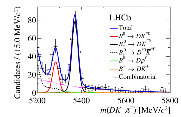
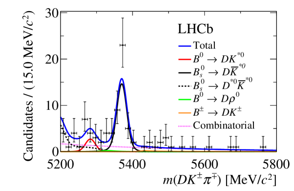
Figure 3: Invariant mass distributions of ${{B}^{0}}\rightarrow D{{K}^{*0}}$ candidates with (top) $D\rightarrow{{K}^{0}_{\mathrm{\scriptscriptstyle S}}}{{\pi}^{+}}{{\pi}^{-}}$ and (bottom) $D\rightarrow{{K}^{0}_{\mathrm{\scriptscriptstyle S}}}{{K}^{+}}{{K}^{-}}$. The fit results, including the signal and background components, are superimposed.

The invariant mass distributions of the selected candidates are shown in Fig. 3 for both $D$ decay modes. The ${B}^{0}$ and ${\kern 1.79993pt\overline{\kern-1.79993ptB}{}}{}^{0}$ candidates are summed. The result of an extended maximum likelihood fit to these distributions is superimposed. The fit is performed simultaneously for candidates from both $D$ decays, allowing parameters, unless otherwise stated, to be common between both $D$ decay categories. Figure 3 shows the various components that are considered in the fit to the invariant mass spectra. In addition to the signal ${{B}^{0}}\rightarrow D{{K}^{*0}}$ component, there are contributions from ${{B}^{0}_{s}}\rightarrow D{{\kern 1.99997pt\overline{\kern-1.99997ptK}{}}{}^{*0}}$, from ${{B}^{0}}\rightarrow D{{\rho}^{0}}$ where one pion is misidentified as a kaon, and from $B\rightarrow DK$ decays where one pion from the rest of the event is added to create a fake ${K}^{*0}$. A large background comes from ${{B}^{0}_{s}}\rightarrow{{D}^{*0}}{{\kern 1.99997pt\overline{\kern-1.99997ptK}{}}{}^{*0}}$ decays where the photon or neutral pion from the ${{D}^{*0}}$ decay is not reconstructed. The purpose of this fit is to determine the parametrisation of the signal and background components, and the size of the background contributions, which are used in the fit of partitioned regions of the Dalitz plot described in Sect. 6.

The ${{B}^{0}_{s}}\rightarrow D{{\kern 1.99997pt\overline{\kern-1.99997ptK}{}}{}^{*0}}$ and ${{B}^{0}}\rightarrow D{{K}^{*0}}$ decays are modelled by the same probability density function (PDF), a sum of two Crystal Ball [48] functions with common mean and width parameters. The mean for the ${B}^{0}_{s}$ meson is determined in the fit and the mean for the ${B}^{0}$ meson is required to be $87.19{\mathrm{\,Me\kern-1.00006ptV\!/}c^{2}}$ [15] lower. The width is allowed to vary in the fit and is required to be the same for the two decays. All other parameters are fixed from simulation. The combinatorial background is modelled by an exponential function with slope determined by the fit for the $D\rightarrow{{K}^{0}_{\mathrm{\scriptscriptstyle S}}}{{\pi}^{+}}{{\pi}^{-}}$ and $D\rightarrow{{K}^{0}_{\mathrm{\scriptscriptstyle S}}}{{K}^{+}}{{K}^{-}}$ categories separately. The PDF for ${{B}^{0}}\rightarrow D{{\rho}^{0}}$ decays is derived from simulation with additional data-driven corrections applied to take into account PID response differences between data and simulation [49]. This background is described with the sum of two Crystal Ball functions, whose parameters are obtained from the weighted simulated events. The $B\rightarrow DK$ background is treated in a similar fashion.

For the partially reconstructed background from ${{B}^{0}_{s}}\rightarrow{{D}^{*0}}{{\kern 1.99997pt\overline{\kern-1.99997ptK}{}}{}^{*0}}$ decays the distribution in the invariant mass spectrum is dependent on the helicity state of the ${D}^{*0}$ meson. The initial decay of the ${B}^{0}_{s}$ involves the decay of a pseudoscalar to two vector particles. Hence, due to angular momentum conservation there are three helicity amplitudes to consider, which can be labelled by the ${D}^{*0}$ helicity state $\lambda=-1,0,+1$. In the subsequent parity-conserving decay ${{D}^{*0}}\rightarrow{{D}^{0}}\{{{\pi}^{0}},\gamma\}$, the value of $\lambda$ and the spin of the missing neutral particle determines the distribution of the ${D}^{*0}$ helicity angle, which is defined as the angle between the missing neutral particle’s momentum vector and the direction opposite to the $B$ meson in the ${D}^{*0}$ rest frame. The resulting distributions for $\lambda=-1$ or $+1$ are identical and hence are grouped together. The functional forms of the underlying $DK\pi$ invariant mass spectrum, shown in Table 1, can be calculated based on $\lambda$, and the spin and mass of the missing particle. The parameters $a_{X}$ and $b_{X}$ are the kinematic endpoints of the reconstructed $DK\pi$ invariant mass, where $X$ is the particle that is not reconstructed. These distributions are further modified to take into account detector resolution and reconstruction efficiency. The parameters for the resolution and efficiency are determined from fits to simulated samples, while the endpoints are calculated using the masses of the particles involved.

Table 1: Functional forms of the $DK\pi$ invariant mass distribution, $m$, in partially reconstructed decays of ${{B}^{0}_{s}}\rightarrow({{D}^{*0}}\rightarrow{{D}^{0}}\{{{\pi}^{0}},\gamma\}){{\kern 1.99997pt\overline{\kern-1.99997ptK}{}}{}^{*0}}$, where either the ${\pi}^{0}$ or $\gamma$ is not reconstructed. The ${D}^{*0}$ helicity state is given by $\lambda$. The quantities $a_{X}$ and $b_{X}$ are the minimum and maximum kinematic boundaries of the reconstructed $DK\pi$ invariant mass, where $X$ is the particle that is missed.

Missed particle	$\lambda$	PDF
${{\pi}^{0}}$	0	$\left(m-\frac{a_{{\pi}^{0}}+b_{{\pi}^{0}}}{2}\right)^{2}$
${{\pi}^{0}}$	$-1$ or $+1$	$-(m-a_{{\pi}^{0}})(m-b_{{\pi}^{0}})$
$\gamma$	0	$-(m-a_{\gamma})(m-b_{\gamma})$
$\gamma$	$-1$ or $+1$	$\left(m-\frac{a_{\gamma}+b_{\gamma}}{2}\right)^{2}+\left(\frac{a_{\gamma}-b_{\gamma}}{2}\right)^{2}$

The lower range of the mass fit is $5200{\mathrm{\,Me\kern-1.00006ptV\!/}c^{2}}$. The removal of candidates with invariant mass below this value reduces the background from ${{B}^{0}}\rightarrow{{D}^{*0}}{{K}^{*0}}$ decays to a small level, which is neglected in the baseline fit. Other contributions such as $B^{\pm}\rightarrow Dh^{\pm}{{\pi}^{+}}{{\pi}^{-}}$, where one particle is missing and another may be misidentified, are also reduced to a negligible level.

With the large number of overlapping signal and background contributions it is not possible to let all yield parameters vary freely, especially as some background contributions are expected to have small yields. Therefore, the strategy employed is to constrain the ratio of these background yields to the ${{B}^{0}_{s}}\rightarrow D{{\kern 1.99997pt\overline{\kern-1.99997ptK}{}}{}^{*0}}$ contribution. The constraints are determined by taking into account all relevant branching fractions [15], fragmentation fractions [50] and selection efficiencies determined from simulation. This is possible for the contributions ${{B}^{0}}\rightarrow D{{\rho}^{0}}$ and $B\rightarrow DK$ where the branching fractions are measured. The ratio of ${{B}^{0}}\rightarrow D{{\rho}^{0}}$ ($B\rightarrow DK$) to ${{B}^{0}_{s}}\rightarrow D{{\kern 1.99997pt\overline{\kern-1.99997ptK}{}}{}^{*0}}$ is constrained in the fit to $R_{\rho}=(2.9\pm 0.8)\%$ ($R_{DK}=(4.2\pm 1.0)\%$). In the case of the ${{B}^{0}_{s}}\rightarrow{{D}^{*0}}{{\kern 1.99997pt\overline{\kern-1.99997ptK}{}}{}^{*0}}$ background, neither its branching fraction nor the relative fraction of the ${{D}^{*0}}$ helicity states has been measured. Therefore, information is taken from the higher statistics ${{B}^{0}_{s}}\rightarrow D(\rightarrow K\pi){{\kern 1.99997pt\overline{\kern-1.99997ptK}{}}{}^{*0}}$ decay, which has been studied by the LHCb collaboration [11]. In these Cabibbo-favoured decays the mass distribution is simpler since the ${{B}^{0}}\rightarrow D{{K}^{*0}}$ and ${{B}^{0}}\rightarrow{{D}^{*0}}{{K}^{*0}}$ decays are doubly Cabibbo-suppressed, hence allowing the shape parameters and yields for the ${{B}^{0}_{s}}\rightarrow D{{\kern 1.99997pt\overline{\kern-1.99997ptK}{}}{}^{*0}}$ and ${{B}^{0}_{s}}\rightarrow{{D}^{*0}}{{\kern 1.99997pt\overline{\kern-1.99997ptK}{}}{}^{*0}}$ decays to be reliably determined. The expected ratio $R_{s}$ between ${{B}^{0}_{s}}\rightarrow{{D}^{*0}}{{\kern 1.99997pt\overline{\kern-1.99997ptK}{}}{}^{*0}}$ and ${{B}^{0}_{s}}\rightarrow D{{\kern 1.99997pt\overline{\kern-1.99997ptK}{}}{}^{*0}}$ can be determined using the information from the analysis of $D\rightarrow K\pi$ decays, with a correction for the selection efficiencies. The ratio between the total yield of the ${{B}^{0}_{s}}\rightarrow{{D}^{*0}}{{\kern 1.99997pt\overline{\kern-1.99997ptK}{}}{}^{*0}}$ candidates with reconstructed mass above $5200{\mathrm{\,Me\kern-1.00006ptV\!/}c^{2}}$ and ${{B}^{0}_{s}}\rightarrow D{{\kern 1.99997pt\overline{\kern-1.99997ptK}{}}{}^{*0}}$ candidates is determined to be $R_{s}=(35\pm 14)\%$. The fraction of ${{B}^{0}_{s}}\rightarrow{{D}^{*0}}{{\kern 1.99997pt\overline{\kern-1.99997ptK}{}}{}^{*0}}$ candidates where $\lambda=0$ is determined to be $\alpha=0.72\pm 0.13$. The yields of the ${{B}^{0}_{s}}\rightarrow D{{\kern 1.99997pt\overline{\kern-1.99997ptK}{}}{}^{*0}}$, ${{B}^{0}}\rightarrow D{{K}^{*0}}$ and the combinatorial background are free parameters in the fit. Pseudoexperiments for this fit configuration show that only negligible biases are expected. The fitted yields and parameters of the fit are given in Table 2. The purity in the signal region, defined as $\pm 25{\mathrm{\,Me\kern-1.00006ptV\!/}c^{2}}$ around the ${B}^{0}$ mass measured in the fit, is 59% (44%) for the ${{K}^{0}_{\mathrm{\scriptscriptstyle S}}}{{\pi}^{+}}{{\pi}^{-}}$ (${{K}^{0}_{\mathrm{\scriptscriptstyle S}}}{{K}^{+}}{{K}^{-}}$) candidates. The background is dominated by combinatorial and ${{B}^{0}_{s}}\rightarrow{{D}^{*0}}{{\kern 1.99997pt\overline{\kern-1.99997ptK}{}}{}^{*0}}$ decays. Contributions from the other backgrounds considered are small.

Table 2: Results of the simultaneous fit to the invariant mass distribution of ${{B}^{0}}\rightarrow D{{K}^{*0}}$ decays, with the $D$ meson decaying to ${{K}^{0}_{\mathrm{\scriptscriptstyle S}}}{{\pi}^{+}}{{\pi}^{-}}$ and ${{K}^{0}_{\mathrm{\scriptscriptstyle S}}}{{K}^{+}}{{K}^{-}}$.

Variable	Fitted value and uncertainty
${B}^{0}_{s}$ mass	$5369.2$	${}^{+1.0}_{-1.0}\;{\mathrm{\,Me\kern-1.00006ptV\!/}c^{2}}$
Signal width parameter	$13.3$	${}^{+1.0}_{-0.9}\;{\mathrm{\,Me\kern-1.00006ptV\!/}c^{2}}$
${{K}^{0}_{\mathrm{\scriptscriptstyle S}}}{{K}^{+}}{{K}^{-}}$ exponential slope	$(-3.4$	${}^{+1.6}_{-1.4})\times 10^{-3}\;(\!{\mathrm{\,Me\kern-1.00006ptV\!/}c^{2}})^{-1}$
${{K}^{0}_{\mathrm{\scriptscriptstyle S}}}{{\pi}^{+}}{{\pi}^{-}}$ exponential slope	$(-5.4$	${}^{+0.9}_{-0.8})\times 10^{-3}\;(\!{\mathrm{\,Me\kern-1.00006ptV\!/}c^{2}})^{-1}$
$\alpha$	$0.74$	${}^{+0.13}_{-0.13}$
$R_{DK}$	$(4.3$	${}^{+1.0}_{-1.0})\times 10^{-2}$
$R_{\rho}$	$(3.0$	${}^{+0.8}_{-0.8})\times 10^{-2}$
$R_{s}$	$0.31$	${}^{+0.09}_{-0.09}$
$n({{B}^{0}}\rightarrow D{{K}^{*0}},{{K}^{0}_{\mathrm{\scriptscriptstyle S}}}{{\pi}^{+}}{{\pi}^{-}})$	$84$	${}^{+15}_{-14}$
$n({{B}^{0}_{s}}\rightarrow D{{\kern 1.99997pt\overline{\kern-1.99997ptK}{}}{}^{*0}},{{K}^{0}_{\mathrm{\scriptscriptstyle S}}}{{\pi}^{+}}{{\pi}^{-}})$	$194$	${}^{+18}_{-17}$
$n(\mathrm{combinatorial},{{K}^{0}_{\mathrm{\scriptscriptstyle S}}}{{\pi}^{+}}{{\pi}^{-}})$	$207$	${}^{+36}_{-35}$
$n({{B}^{0}}\rightarrow D{{K}^{*0}},{{K}^{0}_{\mathrm{\scriptscriptstyle S}}}{{K}^{+}}{{K}^{-}})$	$6.7$	${}^{+4.8}_{-4.2}$
$n({{B}^{0}_{s}}\rightarrow D{{\kern 1.99997pt\overline{\kern-1.99997ptK}{}}{}^{*0}},{{K}^{0}_{\mathrm{\scriptscriptstyle S}}}{{K}^{+}}{{K}^{-}})$	$36.3$	${}^{+7.1}_{-6.4}$
$n(\mathrm{combinatorial},{{K}^{0}_{\mathrm{\scriptscriptstyle S}}}{{K}^{+}}{{K}^{-}})$	$32.3$	${}^{+10.0}_{-9.0}$

The Dalitz plots for ${{B}^{0}}\rightarrow D{{K}^{*0}}$ candidates restricted to the signal region for the two $D\rightarrow{{K}^{0}_{\mathrm{\scriptscriptstyle S}}}h^{+}h^{-}$ final states are shown in Figs. 4 and 5. Separate plots are shown for ${B}^{0}$ and ${\kern 1.79993pt\overline{\kern-1.79993ptB}{}}{}^{0}$ decays.

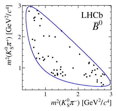
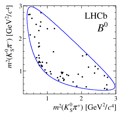
Figure 4: Dalitz plots of candidates in the signal region for $D\rightarrow{{K}^{0}_{\mathrm{\scriptscriptstyle S}}}{{\pi}^{+}}{{\pi}^{-}}$ decays from (left) ${{\kern 1.79993pt\overline{\kern-1.79993ptB}{}}{}^{0}}\rightarrow D{{\kern 1.99997pt\overline{\kern-1.99997ptK}{}}{}^{*0}}$ and (right) ${{B}^{0}}\rightarrow D{{K}^{*0}}$ decays. The solid blue line indicates the kinematic boundary.

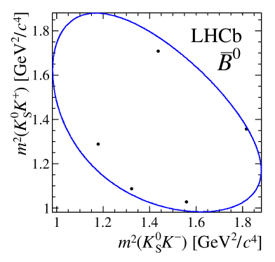
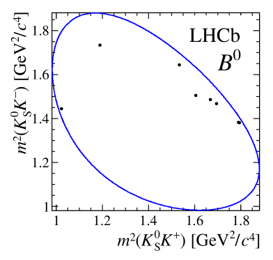
Figure 5: Dalitz plots of candidates in the signal region for $D\rightarrow{{K}^{0}_{\mathrm{\scriptscriptstyle S}}}{{K}^{+}}{{K}^{-}}$ decays from (left) ${{\kern 1.79993pt\overline{\kern-1.79993ptB}{}}{}^{0}}\rightarrow D{{\kern 1.99997pt\overline{\kern-1.99997ptK}{}}{}^{*0}}$ and (right) ${{B}^{0}}\rightarrow D{{K}^{*0}}$ decays. The solid blue line indicates the kinematic boundary.

5 Event selection and yield determination for ${{B}^{0}}\rightarrow{{D}^{*-}}\mu^{+}\nu_{\mu}$ decays

A sample of ${{B}^{0}}\rightarrow{{D}^{*-}}\mu^{+}\nu_{\mu}$, ${{D}^{*-}}\rightarrow{{\kern 1.99997pt\overline{\kern-1.99997ptD}{}}{}^{0}}{{\pi}^{-}}$, ${{\kern 1.99997pt\overline{\kern-1.99997ptD}{}}{}^{0}}\rightarrow{{K}^{0}_{\mathrm{\scriptscriptstyle S}}}h^{+}h^{-}$ decays is used to determine the quantities $F_{i}$, defined in Eq. (12), as the expected fractions of ${D}^{0}$ decays falling into Dalitz plot bin $i$, taking into account the efficiency profile of the signal decay. The semileptonic decay of the $B$ meson and the strong-interaction decay of the ${D}^{*\pm}$ meson allow the flavour of the ${D}^{0}$ meson to be determined from the charge of the muon and ${D}^{*\pm}$ daughter pion. This particular decay chain, involving a flavour-tagged ${D}^{0}$ decay, is chosen due to its high yield, low background level, and low mistag probability. The selection requirements are chosen to minimise changes to the efficiency profile with respect to that associated with the ${{B}^{0}}\rightarrow D{{K}^{*0}}$ channel and are the same as those listed in Ref. [8], with two exceptions. First, only events which pass the hardware trigger that selects muons with a transverse momentum $\mbox{$p_{\mathrm{T}}$}>1.48{\mathrm{\,Ge\kern-1.00006ptV\!/}c}$ are used. Those where the hardware trigger only satisfies the criterion of a high transverse energy deposit in the hadronic calorimeter are not considered. Second, the multivariate algorithm in the software trigger designed to select secondary vertices that are consistent with the decay of a $b$ hadron is identical to the one used for ${{B}^{0}}\rightarrow D{{K}^{*0}}$ candidates; an algorithm that also required the presence of a muon track was previously used. The changes remove approximately $20\%$ of the sample used in Ref. [8]; however, in simulated data they improve the agreement in the variation of the efficiency over the Dalitz plot between the ${{B}^{0}}\rightarrow D{{K}^{*0}}$ and ${{B}^{0}}\rightarrow{{D}^{*-}}\mu^{+}\nu_{\mu}$ decays.

The ${D}^{0}$ invariant mass, $m({{K}^{0}_{\mathrm{\scriptscriptstyle S}}}h^{+}h^{-})$, and the invariant mass difference $\Delta m\equiv m({{K}^{0}_{\mathrm{\scriptscriptstyle S}}}h^{+}h^{-}{{\pi}^{\pm}})-m({{K}^{0}_{\mathrm{\scriptscriptstyle S}}}h^{+}h^{-})$ are fitted simultaneously to determine the signal and background yields. No significant correlation between these two variables is observed within the ranges chosen for the fit. This two-dimensional parametrisation allows the yield of selected candidates to be measured in three categories: true ${{D}^{*\pm}}$ candidates (signal), candidates containing a true ${D}^{0}$ but a random soft pion (RSP) and candidates formed from random track combinations that fall within the fit range (combinatorial background). An example fit projection is shown in Fig. 6. The result of the two-dimensional extended unbinned maximum likelihood fit is superimposed. The fit is performed simultaneously for the two ${D}^{0}$ final states and the two ${K}^{0}_{\mathrm{\scriptscriptstyle S}}$ categories, with some parameters allowed to vary between categories. Candidates selected from data recorded at $\sqrt{s}=7$ and $8\mathrm{\,Te\kern-1.00006ptV}$ are fitted separately, due to their slightly different Dalitz plot efficiency profiles. The fit range is $1830<m({{K}^{0}_{\mathrm{\scriptscriptstyle S}}}h^{+}h^{-})<1910{\mathrm{\,Me\kern-1.00006ptV\!/}c^{2}}$ and $139.5<\Delta m<153.0{\mathrm{\,Me\kern-1.00006ptV\!/}c^{2}}$. The PDFs used to model the various components in the fit are unchanged from those used in Ref. [8], where further details can be found.

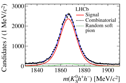
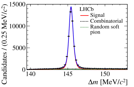
Figure 6: Result of the simultaneous fit to ${{B}^{0}}\rightarrow{{D}^{*-}}\mu^{+}\nu_{\mu}$, ${{D}^{*-}}\rightarrow{{\kern 1.99997pt\overline{\kern-1.99997ptD}{}}{}^{0}}(\rightarrow{{K}^{0}_{\mathrm{\scriptscriptstyle S}}}{{\pi}^{+}}{{\pi}^{-}}){{\pi}^{-}}$ decays with downstream ${K}^{0}_{\mathrm{\scriptscriptstyle S}}$ candidates, in 2012 data. A two-dimensional fit is performed in (left) $m({{K}^{0}_{\mathrm{\scriptscriptstyle S}}}h^{+}h^{-})$ and (right) $\Delta m$. The (blue) total fit PDF and the signal and background components are superimposed.

A total signal yield of approximately 90 000 (12 000) $D\rightarrow{{K}^{0}_{\mathrm{\scriptscriptstyle S}}}{{\pi}^{+}}{{\pi}^{-}}$ ($D\rightarrow{{K}^{0}_{\mathrm{\scriptscriptstyle S}}}{{K}^{+}}{{K}^{-}}$) candidates is obtained. The sample is three orders of magnitude larger than the ${{B}^{0}}\rightarrow D{{K}^{*0}}$ yield. The signal mass range is defined as 1840–$1890{\mathrm{\,Me\kern-1.00006ptV\!/}c^{2}}$ (1850–$1880{\mathrm{\,Me\kern-1.00006ptV\!/}c^{2}}$) in $m({{K}^{0}_{\mathrm{\scriptscriptstyle S}}}{{\pi}^{+}}{{\pi}^{-}})$ ($m({{K}^{0}_{\mathrm{\scriptscriptstyle S}}}{{K}^{+}}{{K}^{-}})$) and 143.9–$146.9{\mathrm{\,Me\kern-1.00006ptV\!/}c^{2}}$ in $\Delta m$. Within this range the background contamination is 3–6% depending on the category.

The two-dimensional fit in $m({{K}^{0}_{\mathrm{\scriptscriptstyle S}}}h^{+}h^{-})$ and $\Delta m$ of the ${{B}^{0}}\rightarrow{{D}^{*-}}\mu^{+}\nu_{\mu}$ decay is repeated in each Dalitz plot bin with all of the PDF parameters fixed, resulting in a raw control mode yield, $R_{i}$, for each bin $i$. The measured $R_{i}$ are not equivalent to the $F_{i}$ fractions required to determine the $C\!P$ parameters due to unavoidable differences from selection criteria in the efficiency profiles of the signal and control modes. Hence, a set of correction factors is determined from simulation. The efficiency profiles from simulation of $D\rightarrow{{K}^{0}_{\mathrm{\scriptscriptstyle S}}}{{\pi}^{+}}{{\pi}^{-}}$ decays are shown in Fig. 7. They show a variation of 50% between the highest and lowest efficiency regions, although the efficiency changes within a bin are not as large. The variation over the $D\rightarrow{{K}^{0}_{\mathrm{\scriptscriptstyle S}}}{{K}^{+}}{{K}^{-}}$ Dalitz plot is smaller, at approximately 35%.

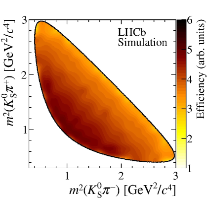
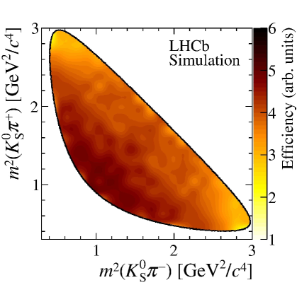
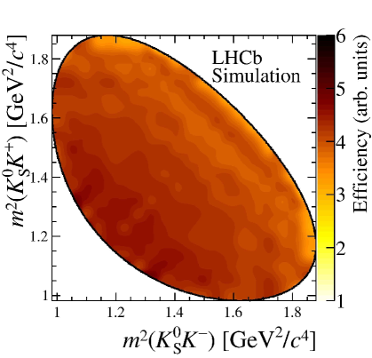
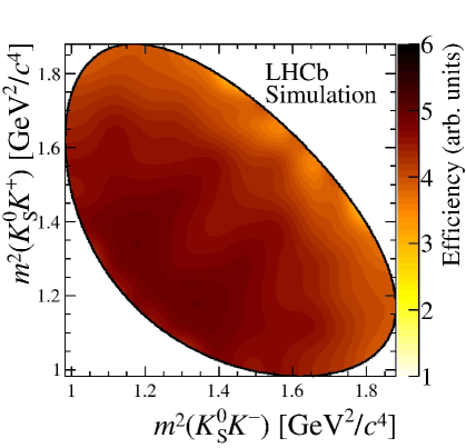
Figure 7: Example efficiency profiles of (left) ${{B}^{0}}\rightarrow D{{K}^{*0}}$ and (right) ${{B}^{0}}\rightarrow{{D}^{*-}}\mu^{+}\nu_{\mu}$ decays in the simulation. The top (bottom) plots are for $D\rightarrow{{K}^{0}_{\mathrm{\scriptscriptstyle S}}}{{\pi}^{+}}{{\pi}^{-}}$ ($D\rightarrow{{K}^{0}_{\mathrm{\scriptscriptstyle S}}}{{K}^{+}}{{K}^{-}}$) decays.

The raw yields of the control decay must be corrected to take into account the differences in efficiency profiles. For each Dalitz plot bin a correction factor is determined,

$$\xi_{i}\equiv\frac{\int_{i}dm^{2}_{-}\,dm^{2}_{+}\,|A_{D}(m^{2}_{-},m^{2}_{+})|^{2}\,\eta_{DK^{*0}}(m^{2}_{-},m^{2}_{+})}{\int_{i}dm^{2}_{-}\,dm^{2}_{+}\,|A_{D}(m^{2}_{-},m^{2}_{+})|^{2}\,\eta_{{{D}^{*}}\mu}(m^{2}_{-},m^{2}_{+})},$$ (13)

where $\eta_{DK^{*0}}$ and $\eta_{{{D}^{*}}\mu}$ are the efficiency profiles of the ${{B}^{0}}\rightarrow D{{K}^{*0}}$ and ${{B}^{0}}\rightarrow{{D}^{*-}}\mu^{+}\nu_{\mu}$ decays, respectively, and are determined with simulation. The amplitude models used to determine the Dalitz plot intensity for the correction factor are those from Ref. [24] and Ref. [25] for the ${{K}^{0}_{\mathrm{\scriptscriptstyle S}}}{{\pi}^{+}}{{\pi}^{-}}$ and ${{K}^{0}_{\mathrm{\scriptscriptstyle S}}}{{K}^{+}}{{K}^{-}}$ decays, respectively. The amplitude models used here only provide a description of the intensity distribution over the Dalitz plot and introduce no significant model dependence into the analysis. The correction factors are determined separately for data reconstructed with each ${K}^{0}_{\mathrm{\scriptscriptstyle S}}$ type, as the efficiency profile is different between the two ${K}^{0}_{\mathrm{\scriptscriptstyle S}}$ categories. This method of determining the $F_{i}$ parameters is preferable to using solely the amplitude models and ${{B}^{0}}\rightarrow D{{K}^{*0}}$ simulated events, since the method is data-driven and the efficiency correction causes deficiencies in the simulation and the model to cancel at first order. The correction factors are within 10$\%$ of unity. The $F_{i}$ values can be determined via the relation $F_{i}=h^{\prime}\xi_{i}R_{i}$, where $h^{\prime}$ is a normalisation factor such that the sum of all $F_{i}$ is unity. The $F_{i}$ parameters are determined for each year of data taking and ${K}^{0}_{\mathrm{\scriptscriptstyle S}}$ category separately and are then combined in the fraction observed in the ${{B}^{0}}\rightarrow D{{K}^{*0}}$ signal region in data. The total uncertainty on $F_{i}$ is 5% or less in all of the bins, and is a combination of the uncertainty on $R_{i}$ due to the size of the control channel, and the uncertainty on $\xi_{i}$ due to the limited size of the simulated samples. The two contributions are similar in size.

6 Dalitz plot fit to determine the $C\!P$-violating parameters $x_{\pm}$ and $y_{\pm}$

The Dalitz plot fit is used to measure the $C\!P$-violating parameters $x_{\pm}$ and $y_{\pm}$, as introduced in Sect. 2. Following Eqs. (10) and (11), these parameters can be determined from the populations of the ${B}^{0}$ and ${\kern 1.79993pt\overline{\kern-1.79993ptB}{}}{}^{0}$ Dalitz plot bins, given the external information of the $c_{i}$ and $s_{i}$ parameters from CLEO-c data, the values of $F_{i}$ from the semileptonic control decay modes and the measured value of $\kappa$.

Although the absolute numbers of ${B}^{0}$ and ${\kern 1.79993pt\overline{\kern-1.79993ptB}{}}{}^{0}$ decays integrated over the $D$ Dalitz plot have some dependence on $x_{\pm}$ and $y_{\pm}$, the sensitivity gained compared to using just the relations in Eqs. (10) and (11) is negligible [51]. Consequently, as stated previously, the integrated yields are not used and the analysis is insensitive to $B$ meson production and detection asymmetries.

The ${{B}^{0}}\rightarrow D{{K}^{*0}}$ data are split into four categories, one for each $D$ decay and then by the charge of the ${K}^{*0}$ daughter kaon. As in the case of the fit to the invariant mass, data from the two ${K}^{0}_{\mathrm{\scriptscriptstyle S}}$ categories are merged. Each category is then divided into the Dalitz plot bins shown in Fig. 2, where there are 16 bins for $D\rightarrow{{K}^{0}_{\mathrm{\scriptscriptstyle S}}}{{\pi}^{+}}{{\pi}^{-}}$ and 4 bins for $D\rightarrow{{K}^{0}_{\mathrm{\scriptscriptstyle S}}}{{K}^{+}}{{K}^{-}}$. Since the Dalitz plots for ${B}^{0}$ and ${\kern 1.79993pt\overline{\kern-1.79993ptB}{}}{}^{0}$ data are analysed separately, this gives a total of 40 bins. The PDF parameters for the signal and background invariant mass distributions are fixed to the values determined in the invariant mass fit described in Sect. 4.

The yield of the combinatorial background in each bin is a free parameter, apart from the yields in bins in which an auxiliary fit determines it to be negligible. It is necessary to set these to zero to facilitate the calculation of the covariance matrix. The total yield of ${{B}^{0}_{s}}\rightarrow D{{\kern 1.99997pt\overline{\kern-1.99997ptK}{}}{}^{*0}}$ decays integrated over the Dalitz plot for each category is a free parameter. The value of $r_{B}({{B}^{0}_{s}}\rightarrow D{{\kern 1.99997pt\overline{\kern-1.99997ptK}{}}{}^{*0}})$ is expected to be an order of magnitude smaller than $r_{{B}^{0}}$ due to suppression from CKM factors. Hence, the fractions in each Dalitz plot bin are assigned assuming that $C\!P$ violation in these decays are negligible, which is also consistent with observations in Ref. [14]. Therefore, the decay of the ${B}^{0}_{s}$ (${\kern 1.79993pt\overline{\kern-1.79993ptB}{}}{}^{0}_{s}$) meson contains a ${\kern 1.99997pt\overline{\kern-1.99997ptD}{}}{}^{0}$ (${D}^{0}$) meson. It is verified in simulation that the reconstruction efficiency over the $D$ Dalitz plot does not depend on the parent $B$ decay and hence the yield of ${{B}^{0}_{s}}\rightarrow D{{\kern 1.99997pt\overline{\kern-1.99997ptK}{}}{}^{*0}}$ decays in bin $i$ is given by the relevant total yield multiplied by $F_{-i}$.

The total yields of the ${{B}^{0}_{s}}\rightarrow{{D}^{*0}}{{\kern 1.99997pt\overline{\kern-1.99997ptK}{}}{}^{*0}}$, ${{B}^{0}}\rightarrow D{{\rho}^{0}}$ and $B\rightarrow DK$ backgrounds in each category are determined by multiplying the total yield of ${{B}^{0}_{s}}\rightarrow D{{\kern 1.99997pt\overline{\kern-1.99997ptK}{}}{}^{*0}}$ in that category by the values of $R_{s}$, $R_{\rho}$ and $R_{DK}$, respectively, that are listed in Table 2. The following assumptions are made about the Dalitz plot distributions of these backgrounds. The $C\!P$ violation in ${{B}^{0}_{s}}\rightarrow{{D}^{*0}}{{\kern 1.99997pt\overline{\kern-1.99997ptK}{}}{}^{*0}}$ decays is expected to be negligible as the underlying CKM factors are the same as that for ${{B}^{0}_{s}}\rightarrow D{{\kern 1.99997pt\overline{\kern-1.99997ptK}{}}{}^{*0}}$ decays. Hence, the ${{B}^{0}_{s}}\rightarrow{{D}^{*0}}{{\kern 1.99997pt\overline{\kern-1.99997ptK}{}}{}^{*0}}$ decays are distributed over the $D\rightarrow{{K}^{0}_{\mathrm{\scriptscriptstyle S}}}h^{+}h^{-}$ Dalitz plot in the same way as ${{B}^{0}_{s}}\rightarrow D{{\kern 1.99997pt\overline{\kern-1.99997ptK}{}}{}^{*0}}$ decays. The $D$ meson from ${{B}^{0}}\rightarrow D{{\rho}^{0}}$ decays is assumed to be an equal admixture of ${D}^{0}$ and ${\kern 1.99997pt\overline{\kern-1.99997ptD}{}}{}^{0}$ and hence the yield is distributed according to ($F_{+i}+F_{-i}$), because the pion misidentified as a kaon is equally likely to be of either charge. In the case of the $B\rightarrow DK$ decay, $C\!P$ violation is expected and the yield is distributed according to Eqs. (10) and (11), where the values of the $C\!P$ violating parameters are those determined in Ref. [8].

The ${{B}^{0}}\rightarrow D{{K}^{*0}}$ yield in each bin is determined using the total yield of ${{B}^{0}}\rightarrow D{{K}^{*0}}$ in each category, which is a free parameter, and Eqs. (10) and (11). The parameters of interest, $x_{\pm}$ and $y_{\pm}$, are allowed to vary. The values of $c_{i}$ and $s_{i}$ are constrained to their measured values from CLEO [23], assuming Gaussian errors and taking into account statistical and systematic correlations. The values of $F_{i}$ are fixed. The value of $\kappa$ is also fixed in the fit to the central value measured in Ref. [14].

An ensemble of 10 000 pseudoexperiments is generated to validate the fit procedure. In each pseudoexperiment the numbers and distributions of signal and background candidates are generated according to the expected distribution in data, taking care to smear the input values of $c_{i}$ and $s_{i}$. The full fit procedure is then performed. A variety of $x_{\pm}$ and $y_{\pm}$ values consistent with previous measurements is used [50]. Small biases in the central values, with magnitudes around $10\%$ of the statistical uncertainty, are observed in the pseudoexperiments. These biases are due to the low event yields in some of the bins and they reduce in simulated experiments with higher yields. The central values are corrected for the biases.

The results of the fit are $x_{+}=0.05\pm 0.35$, $x_{-}=-0.31\pm 0.20$, $y_{+}=-0.81\pm 0.28$, and $y_{-}=0.31\pm 0.21$. The statistical uncertainties are compatible with those predicted by the pseudoexperiments. The measured values of $(x_{\pm},y_{\pm})$ from the fit to data, with their likelihood contours, corresponding to statistical uncertainties only, are displayed in Fig. 8.

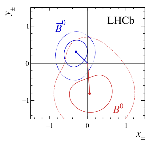
Figure 8: Confidence levels at (solid) 68.3% and (dotted) 95.5% for (red, light) $(x_{+},y_{+})$ and (blue, dark) $(x_{-},y_{-})$ as measured in ${{B}^{0}}\rightarrow D{{K}^{*0}}$ decays (statistical uncertainties only). The parameters $(x_{+},y_{+})$ relate to ${B}^{0}$ decays and $(x_{-},y_{-})$ refer to ${\kern 1.79993pt\overline{\kern-1.79993ptB}{}}{}^{0}$ decays. The points represent the best fit values.

The expected signature for a sample that exhibits $C\!P$ violation is that the two vectors defined by the coordinates $(x_{-},y_{-})$ and $(x_{+},y_{+})$ should both be non-zero in magnitude and have a non-zero opening angle. This opening angle is equal to $2\gamma$. No evidence for $C\!P$ violation is observed.

To investigate whether the binned fit gives an adequate description of the distribution of events over the Dalitz plot, the signal yield in each bin is fitted directly as a cross-check. A comparison of these yields and those predicted by the fitted values of $x_{\pm}$ and $y_{\pm}$ shows good agreement.

7 Systematic uncertainties

Systematic uncertainties are evaluated on the measurements of the Cartesian parameters and are presented in Table 3. The source of each systematic uncertainty is described in turn below. Unless otherwise described, the systematic uncertainties are determined from an ensemble of pseudoexperiments where the simulated data are generated in an alternative configuration, and fitted with the default method described in Sect. 6. The mean shift in the fitted values of $x_{\pm}$ and $y_{\pm}$ in comparison to their input values is taken as the systematic uncertainty. Uncertainties arising from the CLEO measurements are included within the statistical uncertainties since the values of $c_{i}$ and $s_{i}$ are constrained in the Dalitz plot fit. Their contribution to the statistical uncertainty is approximately 0.02 for $x_{\pm}$ and 0.05 for $y_{\pm}$.

Table 3: Summary of the systematic uncertainties for the parameters $x_{\pm},y_{\pm}$. The various sources of systematic uncertainties are described in the main text.

Source	$\sigma(x_{+})$	$\sigma(x_{-})$	$\sigma(y_{+})$	$\sigma(y_{-})$
Efficiency corrections	0.019	0.034	0.021	0.005
Efficiency combination	0.007	0.001	0.007	0.008
Mass fit: $\alpha$	0.002	0.005	0.021	0.020
Mass fit: ${{B}^{0}_{s}}\rightarrow{{D}^{*0}}{{\kern 1.99997pt\overline{\kern-1.99997ptK}{}}{}^{*0}}$	0.002	0.002	0.010	0.005
Mass fit: ${{B}^{0}}\rightarrow D{{\rho}^{0}}$	0.002	0.003	0.004	0.001
Mass fit: $B\rightarrow DK$	0.000	0.000	0.000	0.000
Mass fit: Signal shape	0.005	0.003	0.003	0.002
Mass fit: ${{B}^{0}}\rightarrow{{D}^{*0}}{{K}^{*0}}$	0.006	0.007	0.008	0.004
Mass fit: $B\rightarrow{{D}^{*0}}h$	0.001	0.001	0.007	0.005
Mass fit: $B\rightarrow D\pi\pi\pi$	0.001	0.002	0.001	0.003
Dalitz plot migration	0.003	0.004	0.007	0.003
Value of $\kappa$	0.001	0.011	0.008	0.002
Fitter bias	0.004	0.014	0.042	0.042
Total systematic	0.022	0.040	0.056	0.048

A systematic uncertainty arises from imperfect modelling in the simulation used to derive the efficiency correction in the determination of the $F_{i}$ parameters. To determine this systematic uncertainty, a conservative approach is used, where an alternative set of $F_{i}$ values is determined using only the amplitude models and simulated ${{B}^{0}}\rightarrow D{{K}^{*0}}$ decays. These alternative $F_{i}$ are used in the generation of pseudoexperiments to determine the systematic uncertainty. A further uncertainty on the $F_{i}$ parameters arises from the fractions in which the individual $F_{i}$ parameters from the differing categories (year of data taking and ${K}^{0}_{\mathrm{\scriptscriptstyle S}}$ type) are combined. A second alternate set of $F_{i}$ are obtained by combining the values of $F_{i}$ for each category using the fractions of data observed in the ${B}^{0}_{s}$ mass window. The fractions in the ${B}^{0}$ window are statistically consistent with those observed in the ${B}^{0}_{s}$ mass window. The associated uncertainty is determined through the use of pseudoexperiments which are generated with the alternate set of $F_{i}$ values.

Several systematic uncertainties are associated with the parametrisation of the invariant mass distribution. These arise from uncertainties in the shape of the ${{B}^{0}_{s}}\rightarrow{{D}^{*0}}{{\kern 1.99997pt\overline{\kern-1.99997ptK}{}}{}^{*0}}$ background, the size of the ${{B}^{0}}\rightarrow D{{\rho}^{0}}$ background, $C\!P$ violation in the $B\rightarrow DK$ background, the PDF shape used to describe the signal peak and the inclusion of backgrounds that are neglected in the nominal fit, because of their small yield.

The uncertainty in the shape of the ${{B}^{0}_{s}}\rightarrow{{D}^{*0}}{{\kern 1.99997pt\overline{\kern-1.99997ptK}{}}{}^{*0}}$ background arises from the relative contribution of the different ${D}^{*0}$ decay and helicity state components, each of which have a different $DK\pi$ invariant mass distribution. A different parametrisation of the data with the lower mass limit extending down to 4900${\mathrm{\,Me\kern-1.00006ptV\!/}c^{2}}$ results in a measurement $\alpha=0.9\pm 0.1$, in comparison to the value of $0.74\pm 0.13$ obtained in the fit described in Sect. 4. Accounting for the difference in mass range, the uncertainty is estimated by generating pseudoexperiments with $\alpha=0.91$, and is found to be 2$\times 10^{-3}$ or less in each of the $C\!P$ parameters.

A separate systematic uncertainty is evaluated for the relative fraction of ${{D}^{*0}}\rightarrow{{D}^{0}}{{\pi}^{0}}$ and ${{D}^{*0}}\rightarrow{{D}^{0}}\gamma$ decays in the ${{B}^{0}_{s}}\rightarrow{{D}^{*0}}{{\kern 1.99997pt\overline{\kern-1.99997ptK}{}}{}^{*0}}$ contribution. The uncertainties in the relative fractions are due to uncertainties in the branching fractions of the ${D}^{*0}$ decays and in the selection efficiencies determined in simulation. In this case the systematic uncertainty is small and is determined by fitting the data repeatedly with the fractions smeared around the central values.

The estimation of the ${{B}^{0}}\rightarrow D{{\rho}^{0}}$ yield ignores the ${{B}^{0}}\rightarrow D{{\pi}^{+}}{{\pi}^{-}}$ S-wave contributions, which will contribute if the misidentified ${{\pi}^{+}}{{\pi}^{-}}$ invariant mass falls within the ${K}^{*0}$ mass window. The amplitude analysis of ${{B}^{0}}\rightarrow D{{\pi}^{+}}{{\pi}^{-}}$ decays in Ref. [52] is used to determine that the potential size of the S-wave contribution could increase the apparent ${{B}^{0}}\rightarrow D{{\rho}^{0}}$ yield by approximately 50%. Assuming that the additional S-wave contribution will have the same $DK\pi$ invariant mass distribution, the systematic uncertainty on the $C\!P$ parameters is estimated by generating pseudoexperiments with the ${{B}^{0}}\rightarrow D{{\rho}^{0}}$ contribution increased by 50%. The resulting uncertainties on $x_{\pm},y_{\pm}$ are lower than 4$\times 10^{-3}$.

In the default fit the $C\!P$ parameters of the $B\rightarrow DK$ background are fixed to the central values measured in Ref. [8]. The fits to the data are repeated with multiple values of the $C\!P$ parameters of the $B\rightarrow DK$ decay, smeared according to the measured uncertainties and correlations, and the shifts in $x_{\pm},y_{\pm}$ are found to be less than 0.001.

An alternative PDF to describe the ${B}^{0}$ and ${B}^{0}_{s}$ signals is considered by taking the sum of three Gaussian functions. The mean and width of the primary Gaussian is determined by performing a mass fit to data with the relative means and widths of the two secondary Gaussians taken from simulation. The systematic uncertainty is small and is estimated by generating pseudoexperiments with this alternative PDF.

In the default mass fit the contributions of ${{B}^{0}}\rightarrow{{D}^{*0}}{{K}^{*0}}$, $B^{\pm}\rightarrow{{D}^{*0}}\pi^{\pm}$, $B^{\pm}\rightarrow{{D}^{*0}}K^{\pm}$ and $B^{\pm}\rightarrow D{{\pi}^{\pm}}{{\pi}^{+}}{{\pi}^{-}}$ decays are ignored as they are estimated to contribute approximately $2-3$ events each. A systematic uncertainty from neglecting each of these decays is evaluated. The ${{B}^{0}}\rightarrow{{D}^{*0}}{{K}^{*0}}$ decays can be described with the same PDFs as the ${{B}^{0}_{s}}\rightarrow{{D}^{*0}}{{\kern 1.99997pt\overline{\kern-1.99997ptK}{}}{}^{*0}}$ decays but shifted by the ${{B}^{0}_{s}}-{{B}^{0}}$ mass difference. The $B$ mass fit described in Sect. 4 is performed with this background included, where the yield of ${{B}^{0}}\rightarrow{{D}^{*0}}{{K}^{*0}}$ decays is constrained relative to that of the ${{B}^{0}_{s}}\rightarrow D{{\kern 1.99997pt\overline{\kern-1.99997ptK}{}}{}^{*0}}$ in a similar manner to the ${{B}^{0}_{s}}\rightarrow{{D}^{*0}}{{\kern 1.99997pt\overline{\kern-1.99997ptK}{}}{}^{*0}}$ decays. Although the addition of this background only has a small impact on the mass fit parameters, its $C\!P$ parameters are unknown. Hence, pseudoexperiments are generated with the ${{B}^{0}}\rightarrow{{D}^{*0}}{{K}^{*0}}$ background in three different $C\!P$ violating hypotheses and are fitted with the default configuration. The uncertainty is found to be less than 0.01 for all choices of the $C\!P$ parameters. Further pseudoexperiments are generated with $B^{\pm}\rightarrow{{D}^{*0}}h^{\pm}$ and $B^{\pm}\rightarrow D{{\pi}^{\pm}}{{\pi}^{+}}{{\pi}^{-}}$ decays, where their PDF shapes and yields are determined from simulation. Fitting the pseudoexperiments with the nominal fit demonstrates that the uncertainty due to ignoring these decays is 7$\times 10^{-3}$ or less for all $C\!P$ parameters.

The systematic uncertainty from the effect of candidates being assigned the wrong Dalitz plot bin number is considered. This can occur if reconstruction effects cause shifts in the measured values of $m^{2}_{+}$ and $m^{2}_{-}$ away from their true values. For both ${{B}^{0}}\rightarrow D{{K}^{*0}}$ and ${{B}^{0}}\rightarrow{{D}^{*-}}\mu^{+}\nu_{\mu}$ decays the resolution in $m^{2}_{+}$ and $m^{2}_{-}$ is approximately $0.005{\mathrm{\,Ge\kern-1.00006ptV^{2}\!/}c^{4}}$ ($0.006{\mathrm{\,Ge\kern-1.00006ptV^{2}\!/}c^{4}}$) for candidates with long (downstream) ${K}^{0}_{\mathrm{\scriptscriptstyle S}}$ decays. This is small compared to the typical width of a bin, but net migration can occur if the candidate lies close to the edge of a Dalitz plot bin. To first order, this effect is accounted for by use of the control channel, but residual effects enter due to the non-zero value of $r_{{B}^{0}}$ in the signal decay, causing a different distribution in the Dalitz plot. The uncertainty due to these residual effects is determined via pseudoexperiments, in which different input $F_{i}$ values are used to reflect the residual migration. The size of this possible bias is found to vary between 3$\times 10^{-3}$ and 7$\times 10^{-3}$.

The value of $\kappa$ has an associated uncertainty, and so pseudoexperiments are generated assuming the value $\kappa=0.912$, which corresponds to the central value of $\kappa$ lowered by one standard deviation. The mean shifts in $x_{\pm},y_{\pm}$ are of order 0.01. As described in Sect. 6, the central values of the fit parameters $x_{\pm}$ and $y_{\pm}$ are corrected by a fitter bias that is determined with pseudoexperiments. The systematic uncertainty is assigned using half the size of the correction.

The total experimental systematic uncertainty is determined by adding all sources in quadrature and is 0.02 on $x_{+}$, 0.04 on $x_{-}$, 0.06 on $y_{+}$, and 0.05 on $y_{-}$. These uncertainties are dominated by the efficiency corrections in $F_{i}$ and the fitter bias. The systematic uncertainties are less than 20% of the corresponding statistical uncertainties.

8 Results and interpretation

The results for $x_{\pm}$ and $y_{\pm}$ are

$$x_{+} =\phantom{-}0.05\pm 0.35\pm 0.02,$$

$$x_{-} =-0.31\pm 0.20\pm 0.04,$$

$$y_{+} =-0.81\pm 0.28\pm 0.06,$$

$$y_{-} =\phantom{-}0.31\pm 0.21\pm 0.05,$$

where the first uncertainties are statistical and the second are systematic. After accounting for all sources of uncertainty, the correlation matrix between the measured $x_{\pm}$, $y_{\pm}$ parameters for the full data set is obtained, and is given in Table 4. Correlations for the statistical uncertainties are determined by the fit. The systematic uncertainties are only weakly correlated and the correlations are ignored.

Table 4: Total correlation matrix, including statistical and systematic uncertainties, between the $x_{\pm}$, $y_{\pm}$ parameters used in the extraction of $\gamma$.

	$x_{+}$	$x_{-}$	$y_{+}$	$y_{-}$
$x_{+}$	$\phantom{-}1.00$	$\phantom{-}0.00$	$\phantom{-}0.13$	$-0.01$
$x_{-}$		$\phantom{-}1.00$	$-0.01$	$\phantom{-}0.14$
$y_{+}$			$\phantom{-}1.00$	$\phantom{-}0.02$
$y_{-}$				$\phantom{-}1.00$

The results for $x_{\pm}$ and $y_{\pm}$ can be interpreted in terms of the underlying physics parameters $\gamma$, $r_{{{B}^{0}}}$ and $\delta_{{{B}^{0}}}$. This interpretation is performed using a Neyman construction with Feldman-Cousins ordering [53], using the same procedure as described in Ref. [27], yielding confidence levels for the three physics parameters.

In Fig. 9, the projections of the three-dimensional surfaces containing the one and two standard deviation volumes (i.e., $\Delta\chi^{2}=1$ and 4) onto the $(\gamma,r_{{{B}^{0}}})$ and $(\gamma,\delta_{{{B}^{0}}})$ planes are shown; the statistical and systematic uncertainties on $x_{\pm}$ and $y_{\pm}$ are combined in quadrature. The solution for the physics parameters has a two-fold ambiguity, with a second solution corresponding to $(\gamma,\delta_{{{B}^{0}}})\rightarrow(\gamma+180^{\circ},\delta_{{{B}^{0}}}+180^{\circ})$. For the solution that satisfies $0<\gamma<180^{\circ}$, the following results are obtained:

$$r_{{{B}^{0}}} =0.56\pm 0.17,$$

$$\delta_{{{B}^{0}}} =(204\,^{+21}_{-20})^{\circ},$$

$$\gamma =(71\pm 20)^{\circ}.$$

The central value for $\gamma$ is consistent with the world average from previous measurements [5, 6]. The value for $r_{{{B}^{0}}}$, while consistent with current knowledge, has a central value that is larger than expected [16, 17, 26, 24]. The results are also consistent with, but cannot be combined with, the model-dependent analysis of the same dataset performed by LHCb [22].

A key advantage of having direct measurements of $x_{\pm}$ and $y_{\pm}$ is that there is only a two-fold ambiguity in the value of $\gamma$ from the trigonometric expressions. This means that when combined with the results of other $C\!P$ violation studies in ${{B}^{0}}\rightarrow D{{K}^{*0}}$ decays such as those in Ref. [11], these measurements will provide strong constraints on the hadronic parameters, and will provide improved sensitivity to $\gamma$ when combined with all other measurements.

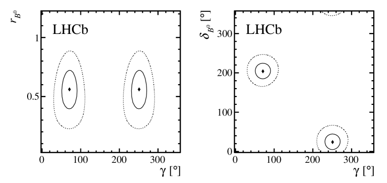
Figure 9: The three-dimensional confidence volumes projected onto the $(\gamma,r_{{{B}^{0}}})$ and $(\gamma,\delta_{{{B}^{0}}})$ planes. The confidence levels correspond to 68.3% and 95.5% confidence levels when projected onto one dimension and are denoted by solid and dotted contours, respectively. The diamonds mark the central values.

LHCb collaboration

R. Aaij³⁹, C. Abellán Beteta⁴¹, B. Adeva³⁸, M. Adinolfi⁴⁷, Z. Ajaltouni⁵, S. Akar⁶, J. Albrecht¹⁰, F. Alessio³⁹, M. Alexander⁵², S. Ali⁴², G. Alkhazov³¹, P. Alvarez Cartelle⁵⁴, A.A. Alves Jr⁵⁸, S. Amato², S. Amerio²³, Y. Amhis⁷, L. An^3,40, L. Anderlini¹⁸, G. Andreassi⁴⁰, M. Andreotti^17,g, J.E. Andrews⁵⁹, R.B. Appleby⁵⁵, O. Aquines Gutierrez¹¹, F. Archilli³⁹, P. d’Argent¹², A. Artamonov³⁶, M. Artuso⁶⁰, E. Aslanides⁶, G. Auriemma^26,n, M. Baalouch⁵, S. Bachmann¹², J.J. Back⁴⁹, A. Badalov³⁷, C. Baesso⁶¹, S. Baker⁵⁴, W. Baldini¹⁷, R.J. Barlow⁵⁵, C. Barschel³⁹, S. Barsuk⁷, W. Barter³⁹, V. Batozskaya²⁹, V. Battista⁴⁰, A. Bay⁴⁰, L. Beaucourt⁴, J. Beddow⁵², F. Bedeschi²⁴, I. Bediaga¹, L.J. Bel⁴², V. Bellee⁴⁰, N. Belloli^21,k, I. Belyaev³², E. Ben-Haim⁸, G. Bencivenni¹⁹, S. Benson³⁹, J. Benton⁴⁷, A. Berezhnoy³³, R. Bernet⁴¹, A. Bertolin²³, F. Betti¹⁵, M.-O. Bettler³⁹, M. van Beuzekom⁴², S. Bifani⁴⁶, P. Billoir⁸, T. Bird⁵⁵, A. Birnkraut¹⁰, A. Bizzeti^18,i, T. Blake⁴⁹, F. Blanc⁴⁰, J. Blouw¹¹, S. Blusk⁶⁰, V. Bocci²⁶, A. Bondar³⁵, N. Bondar^31,39, W. Bonivento¹⁶, A. Borgheresi^21,k, S. Borghi⁵⁵, M. Borisyak⁶⁷, M. Borsato³⁸, M. Boubdir⁹, T.J.V. Bowcock⁵³, E. Bowen⁴¹, C. Bozzi^17,39, S. Braun¹², M. Britsch¹², T. Britton⁶⁰, J. Brodzicka⁵⁵, E. Buchanan⁴⁷, C. Burr⁵⁵, A. Bursche², J. Buytaert³⁹, S. Cadeddu¹⁶, R. Calabrese^17,g, M. Calvi^21,k, M. Calvo Gomez^37,p, P. Campana¹⁹, D. Campora Perez³⁹, L. Capriotti⁵⁵, A. Carbone^15,e, G. Carboni^25,l, R. Cardinale^20,j, A. Cardini¹⁶, P. Carniti^21,k, L. Carson⁵¹, K. Carvalho Akiba², G. Casse⁵³, L. Cassina^21,k, L. Castillo Garcia⁴⁰, M. Cattaneo³⁹, Ch. Cauet¹⁰, G. Cavallero²⁰, R. Cenci^24,t, M. Charles⁸, Ph. Charpentier³⁹, G. Chatzikonstantinidis⁴⁶, M. Chefdeville⁴, S. Chen⁵⁵, S.-F. Cheung⁵⁶, V. Chobanova³⁸, M. Chrzaszcz^41,27, X. Cid Vidal³⁹, G. Ciezarek⁴², P.E.L. Clarke⁵¹, M. Clemencic³⁹, H.V. Cliff⁴⁸, J. Closier³⁹, V. Coco⁵⁸, J. Cogan⁶, E. Cogneras⁵, V. Cogoni^16,f, L. Cojocariu³⁰, G. Collazuol^23,r, P. Collins³⁹, A. Comerma-Montells¹², A. Contu³⁹, A. Cook⁴⁷, S. Coquereau⁸, G. Corti³⁹, M. Corvo^17,g, B. Couturier³⁹, G.A. Cowan⁵¹, D.C. Craik⁵¹, A. Crocombe⁴⁹, M. Cruz Torres⁶¹, S. Cunliffe⁵⁴, R. Currie⁵⁴, C. D’Ambrosio³⁹, E. Dall’Occo⁴², J. Dalseno⁴⁷, P.N.Y. David⁴², A. Davis⁵⁸, O. De Aguiar Francisco², K. De Bruyn⁶, S. De Capua⁵⁵, M. De Cian¹², J.M. De Miranda¹, L. De Paula², P. De Simone¹⁹, C.-T. Dean⁵², D. Decamp⁴, M. Deckenhoff¹⁰, L. Del Buono⁸, N. Déléage⁴, M. Demmer¹⁰, D. Derkach⁶⁷, O. Deschamps⁵, F. Dettori³⁹, B. Dey²², A. Di Canto³⁹, H. Dijkstra³⁹, F. Dordei³⁹, M. Dorigo⁴⁰, A. Dosil Suárez³⁸, A. Dovbnya⁴⁴, K. Dreimanis⁵³, L. Dufour⁴², G. Dujany⁵⁵, K. Dungs³⁹, P. Durante³⁹, R. Dzhelyadin³⁶, A. Dziurda²⁷, A. Dzyuba³¹, S. Easo^50,39, U. Egede⁵⁴, V. Egorychev³², S. Eidelman³⁵, S. Eisenhardt⁵¹, U. Eitschberger¹⁰, R. Ekelhof¹⁰, L. Eklund⁵², I. El Rifai⁵, Ch. Elsasser⁴¹, S. Ely⁶⁰, S. Esen¹², H.M. Evans⁴⁸, T. Evans⁵⁶, A. Falabella¹⁵, C. Färber³⁹, N. Farley⁴⁶, S. Farry⁵³, R. Fay⁵³, D. Fazzini^21,k, D. Ferguson⁵¹, V. Fernandez Albor³⁸, F. Ferrari¹⁵, F. Ferreira Rodrigues¹, M. Ferro-Luzzi³⁹, S. Filippov³⁴, M. Fiore^17,g, M. Fiorini^17,g, M. Firlej²⁸, C. Fitzpatrick⁴⁰, T. Fiutowski²⁸, F. Fleuret^7,b, K. Fohl³⁹, M. Fontana¹⁶, F. Fontanelli^20,j, D. C. Forshaw⁶⁰, R. Forty³⁹, M. Frank³⁹, C. Frei³⁹, M. Frosini¹⁸, J. Fu²², E. Furfaro^25,l, A. Gallas Torreira³⁸, D. Galli^15,e, S. Gallorini²³, S. Gambetta⁵¹, M. Gandelman², P. Gandini⁵⁶, Y. Gao³, J. García Pardiñas³⁸, J. Garra Tico⁴⁸, L. Garrido³⁷, P.J. Garsed⁴⁸, D. Gascon³⁷, C. Gaspar³⁹, L. Gavardi¹⁰, G. Gazzoni⁵, D. Gerick¹², E. Gersabeck¹², M. Gersabeck⁵⁵, T. Gershon⁴⁹, Ph. Ghez⁴, S. Gianì⁴⁰, V. Gibson⁴⁸, O.G. Girard⁴⁰, L. Giubega³⁰, V.V. Gligorov³⁹, C. Göbel⁶¹, D. Golubkov³², A. Golutvin^54,39, A. Gomes^1,a, C. Gotti^21,k, M. Grabalosa Gándara⁵, R. Graciani Diaz³⁷, L.A. Granado Cardoso³⁹, E. Graugés³⁷, E. Graverini⁴¹, G. Graziani¹⁸, A. Grecu³⁰, P. Griffith⁴⁶, L. Grillo¹², O. Grünberg⁶⁵, E. Gushchin³⁴, Yu. Guz^36,39, T. Gys³⁹, T. Hadavizadeh⁵⁶, C. Hadjivasiliou⁶⁰, G. Haefeli⁴⁰, C. Haen³⁹, S.C. Haines⁴⁸, S. Hall⁵⁴, B. Hamilton⁵⁹, X. Han¹², S. Hansmann-Menzemer¹², N. Harnew⁵⁶, S.T. Harnew⁴⁷, J. Harrison⁵⁵, J. He³⁹, T. Head⁴⁰, A. Heister⁹, K. Hennessy⁵³, P. Henrard⁵, L. Henry⁸, J.A. Hernando Morata³⁸, E. van Herwijnen³⁹, M. Heß⁶⁵, A. Hicheur², D. Hill⁵⁶, M. Hoballah⁵, C. Hombach⁵⁵, L. Hongming⁴⁰, W. Hulsbergen⁴², T. Humair⁵⁴, M. Hushchyn⁶⁷, N. Hussain⁵⁶, D. Hutchcroft⁵³, M. Idzik²⁸, P. Ilten⁵⁷, R. Jacobsson³⁹, A. Jaeger¹², J. Jalocha⁵⁶, E. Jans⁴², A. Jawahery⁵⁹, M. John⁵⁶, D. Johnson³⁹, C.R. Jones⁴⁸, C. Joram³⁹, B. Jost³⁹, N. Jurik⁶⁰, S. Kandybei⁴⁴, W. Kanso⁶, M. Karacson³⁹, T.M. Karbach^39,†, S. Karodia⁵², M. Kecke¹², M. Kelsey⁶⁰, I.R. Kenyon⁴⁶, M. Kenzie³⁹, T. Ketel⁴³, E. Khairullin⁶⁷, B. Khanji^21,39,k, C. Khurewathanakul⁴⁰, T. Kirn⁹, S. Klaver⁵⁵, K. Klimaszewski²⁹, M. Kolpin¹², I. Komarov⁴⁰, R.F. Koopman⁴³, P. Koppenburg⁴², M. Kozeiha⁵, L. Kravchuk³⁴, K. Kreplin¹², M. Kreps⁴⁹, P. Krokovny³⁵, F. Kruse¹⁰, W. Krzemien²⁹, W. Kucewicz^27,o, M. Kucharczyk²⁷, V. Kudryavtsev³⁵, A. K. Kuonen⁴⁰, K. Kurek²⁹, T. Kvaratskheliya³², D. Lacarrere³⁹, G. Lafferty^55,39, A. Lai¹⁶, D. Lambert⁵¹, G. Lanfranchi¹⁹, C. Langenbruch⁴⁹, B. Langhans³⁹, T. Latham⁴⁹, C. Lazzeroni⁴⁶, R. Le Gac⁶, J. van Leerdam⁴², J.-P. Lees⁴, R. Lefèvre⁵, A. Leflat^33,39, J. Lefrançois⁷, E. Lemos Cid³⁸, O. Leroy⁶, T. Lesiak²⁷, B. Leverington¹², Y. Li⁷, T. Likhomanenko^67,66, R. Lindner³⁹, C. Linn³⁹, F. Lionetto⁴¹, B. Liu¹⁶, X. Liu³, D. Loh⁴⁹, I. Longstaff⁵², J.H. Lopes², D. Lucchesi^23,r, M. Lucio Martinez³⁸, H. Luo⁵¹, A. Lupato²³, E. Luppi^17,g, O. Lupton⁵⁶, N. Lusardi²², A. Lusiani²⁴, X. Lyu⁶², F. Machefert⁷, F. Maciuc³⁰, O. Maev³¹, K. Maguire⁵⁵, S. Malde⁵⁶, A. Malinin⁶⁶, G. Manca⁷, G. Mancinelli⁶, P. Manning⁶⁰, A. Mapelli³⁹, J. Maratas⁵, J.F. Marchand⁴, U. Marconi¹⁵, C. Marin Benito³⁷, P. Marino^24,t, J. Marks¹², G. Martellotti²⁶, M. Martin⁶, M. Martinelli⁴⁰, D. Martinez Santos³⁸, F. Martinez Vidal⁶⁸, D. Martins Tostes², L.M. Massacrier⁷, A. Massafferri¹, R. Matev³⁹, A. Mathad⁴⁹, Z. Mathe³⁹, C. Matteuzzi²¹, A. Mauri⁴¹, B. Maurin⁴⁰, A. Mazurov⁴⁶, M. McCann⁵⁴, J. McCarthy⁴⁶, A. McNab⁵⁵, R. McNulty¹³, B. Meadows⁵⁸, F. Meier¹⁰, M. Meissner¹², D. Melnychuk²⁹, M. Merk⁴², A Merli^22,u, E Michielin²³, D.A. Milanes⁶⁴, M.-N. Minard⁴, D.S. Mitzel¹², J. Molina Rodriguez⁶¹, I.A. Monroy⁶⁴, S. Monteil⁵, M. Morandin²³, P. Morawski²⁸, A. Mordà⁶, M.J. Morello^24,t, J. Moron²⁸, A.B. Morris⁵¹, R. Mountain⁶⁰, F. Muheim⁵¹, D. Müller⁵⁵, J. Müller¹⁰, K. Müller⁴¹, V. Müller¹⁰, M. Mussini¹⁵, B. Muster⁴⁰, P. Naik⁴⁷, T. Nakada⁴⁰, R. Nandakumar⁵⁰, A. Nandi⁵⁶, I. Nasteva², M. Needham⁵¹, N. Neri²², S. Neubert¹², N. Neufeld³⁹, M. Neuner¹², A.D. Nguyen⁴⁰, C. Nguyen-Mau^40,q, V. Niess⁵, S. Nieswand⁹, R. Niet¹⁰, N. Nikitin³³, T. Nikodem¹², A. Novoselov³⁶, D.P. O’Hanlon⁴⁹, A. Oblakowska-Mucha²⁸, V. Obraztsov³⁶, S. Ogilvy⁵², O. Okhrimenko⁴⁵, R. Oldeman^16,48,f, C.J.G. Onderwater⁶⁹, B. Osorio Rodrigues¹, J.M. Otalora Goicochea², A. Otto³⁹, P. Owen⁵⁴, A. Oyanguren⁶⁸, A. Palano^14,d, F. Palombo^22,u, M. Palutan¹⁹, J. Panman³⁹, A. Papanestis⁵⁰, M. Pappagallo⁵², L.L. Pappalardo^17,g, C. Pappenheimer⁵⁸, W. Parker⁵⁹, C. Parkes⁵⁵, G. Passaleva¹⁸, G.D. Patel⁵³, M. Patel⁵⁴, C. Patrignani^20,j, A. Pearce^55,50, A. Pellegrino⁴², G. Penso^26,m, M. Pepe Altarelli³⁹, S. Perazzini^15,e, P. Perret⁵, L. Pescatore⁴⁶, K. Petridis⁴⁷, A. Petrolini^20,j, M. Petruzzo²², E. Picatoste Olloqui³⁷, B. Pietrzyk⁴, M. Pikies²⁷, D. Pinci²⁶, A. Pistone²⁰, A. Piucci¹², S. Playfer⁵¹, M. Plo Casasus³⁸, T. Poikela³⁹, F. Polci⁸, A. Poluektov^49,35, I. Polyakov³², E. Polycarpo², A. Popov³⁶, D. Popov^11,39, B. Popovici³⁰, C. Potterat², E. Price⁴⁷, J.D. Price⁵³, J. Prisciandaro³⁸, A. Pritchard⁵³, C. Prouve⁴⁷, V. Pugatch⁴⁵, A. Puig Navarro⁴⁰, G. Punzi^24,s, W. Qian⁵⁶, R. Quagliani^7,47, B. Rachwal²⁷, J.H. Rademacker⁴⁷, M. Rama²⁴, M. Ramos Pernas³⁸, M.S. Rangel², I. Raniuk⁴⁴, G. Raven⁴³, F. Redi⁵⁴, S. Reichert¹⁰, A.C. dos Reis¹, V. Renaudin⁷, S. Ricciardi⁵⁰, S. Richards⁴⁷, M. Rihl³⁹, K. Rinnert^53,39, V. Rives Molina³⁷, P. Robbe⁷, A.B. Rodrigues¹, E. Rodrigues⁵⁸, J.A. Rodriguez Lopez⁶⁴, P. Rodriguez Perez⁵⁵, A. Rogozhnikov⁶⁷, S. Roiser³⁹, V. Romanovsky³⁶, A. Romero Vidal³⁸, J. W. Ronayne¹³, M. Rotondo²³, T. Ruf³⁹, P. Ruiz Valls⁶⁸, J.J. Saborido Silva³⁸, N. Sagidova³¹, B. Saitta^16,f, V. Salustino Guimaraes², C. Sanchez Mayordomo⁶⁸, B. Sanmartin Sedes³⁸, R. Santacesaria²⁶, C. Santamarina Rios³⁸, M. Santimaria¹⁹, E. Santovetti^25,l, A. Sarti^19,m, C. Satriano^26,n, A. Satta²⁵, D.M. Saunders⁴⁷, D. Savrina^32,33, S. Schael⁹, M. Schiller³⁹, H. Schindler³⁹, M. Schlupp¹⁰, M. Schmelling¹¹, T. Schmelzer¹⁰, B. Schmidt³⁹, O. Schneider⁴⁰, A. Schopper³⁹, M. Schubiger⁴⁰, M.-H. Schune⁷, R. Schwemmer³⁹, B. Sciascia¹⁹, A. Sciubba^26,m, A. Semennikov³², A. Sergi⁴⁶, N. Serra⁴¹, J. Serrano⁶, L. Sestini²³, P. Seyfert²¹, M. Shapkin³⁶, I. Shapoval^17,44,g, Y. Shcheglov³¹, T. Shears⁵³, L. Shekhtman³⁵, V. Shevchenko⁶⁶, A. Shires¹⁰, B.G. Siddi¹⁷, R. Silva Coutinho⁴¹, L. Silva de Oliveira², G. Simi^23,s, M. Sirendi⁴⁸, N. Skidmore⁴⁷, T. Skwarnicki⁶⁰, E. Smith⁵⁴, I.T. Smith⁵¹, J. Smith⁴⁸, M. Smith⁵⁵, H. Snoek⁴², M.D. Sokoloff⁵⁸, F.J.P. Soler⁵², F. Soomro⁴⁰, D. Souza⁴⁷, B. Souza De Paula², B. Spaan¹⁰, P. Spradlin⁵², S. Sridharan³⁹, F. Stagni³⁹, M. Stahl¹², S. Stahl³⁹, S. Stefkova⁵⁴, O. Steinkamp⁴¹, O. Stenyakin³⁶, S. Stevenson⁵⁶, S. Stoica³⁰, S. Stone⁶⁰, B. Storaci⁴¹, S. Stracka^24,t, M. Straticiuc³⁰, U. Straumann⁴¹, L. Sun⁵⁸, W. Sutcliffe⁵⁴, K. Swientek²⁸, S. Swientek¹⁰, V. Syropoulos⁴³, M. Szczekowski²⁹, T. Szumlak²⁸, S. T’Jampens⁴, A. Tayduganov⁶, T. Tekampe¹⁰, G. Tellarini^17,g, F. Teubert³⁹, C. Thomas⁵⁶, E. Thomas³⁹, J. van Tilburg⁴², V. Tisserand⁴, M. Tobin⁴⁰, S. Tolk⁴³, L. Tomassetti^17,g, D. Tonelli³⁹, S. Topp-Joergensen⁵⁶, E. Tournefier⁴, S. Tourneur⁴⁰, K. Trabelsi⁴⁰, M. Traill⁵², M.T. Tran⁴⁰, M. Tresch⁴¹, A. Trisovic³⁹, A. Tsaregorodtsev⁶, P. Tsopelas⁴², N. Tuning^42,39, A. Ukleja²⁹, A. Ustyuzhanin^67,66, U. Uwer¹², C. Vacca^16,39,f, V. Vagnoni^15,39, S. Valat³⁹, G. Valenti¹⁵, A. Vallier⁷, R. Vazquez Gomez¹⁹, P. Vazquez Regueiro³⁸, C. Vázquez Sierra³⁸, S. Vecchi¹⁷, M. van Veghel⁴², J.J. Velthuis⁴⁷, M. Veltri^18,h, G. Veneziano⁴⁰, M. Vesterinen¹², B. Viaud⁷, D. Vieira², M. Vieites Diaz³⁸, X. Vilasis-Cardona^37,p, V. Volkov³³, A. Vollhardt⁴¹, D. Voong⁴⁷, A. Vorobyev³¹, V. Vorobyev³⁵, C. Voß⁶⁵, J.A. de Vries⁴², R. Waldi⁶⁵, C. Wallace⁴⁹, R. Wallace¹³, J. Walsh²⁴, J. Wang⁶⁰, D.R. Ward⁴⁸, N.K. Watson⁴⁶, D. Websdale⁵⁴, A. Weiden⁴¹, M. Whitehead³⁹, J. Wicht⁴⁹, G. Wilkinson^56,39, M. Wilkinson⁶⁰, M. Williams³⁹, M.P. Williams⁴⁶, M. Williams⁵⁷, T. Williams⁴⁶, F.F. Wilson⁵⁰, J. Wimberley⁵⁹, J. Wishahi¹⁰, W. Wislicki²⁹, M. Witek²⁷, G. Wormser⁷, S.A. Wotton⁴⁸, K. Wraight⁵², S. Wright⁴⁸, K. Wyllie³⁹, Y. Xie⁶³, Z. Xu⁴⁰, Z. Yang³, H. Yin⁶³, J. Yu⁶³, X. Yuan³⁵, O. Yushchenko³⁶, M. Zangoli¹⁵, M. Zavertyaev^11,c, L. Zhang³, Y. Zhang³, A. Zhelezov¹², Y. Zheng⁶², A. Zhokhov³², L. Zhong³, V. Zhukov⁹, S. Zucchelli¹⁵.

¹Centro Brasileiro de Pesquisas Físicas (CBPF), Rio de Janeiro, Brazil
²Universidade Federal do Rio de Janeiro (UFRJ), Rio de Janeiro, Brazil
³Center for High Energy Physics, Tsinghua University, Beijing, China
⁴LAPP, Université Savoie Mont-Blanc, CNRS/IN2P3, Annecy-Le-Vieux, France
⁵Clermont Université, Université Blaise Pascal, CNRS/IN2P3, LPC, Clermont-Ferrand, France
⁶CPPM, Aix-Marseille Université, CNRS/IN2P3, Marseille, France
⁷LAL, Université Paris-Sud, CNRS/IN2P3, Orsay, France
⁸LPNHE, Université Pierre et Marie Curie, Université Paris Diderot, CNRS/IN2P3, Paris, France
⁹I. Physikalisches Institut, RWTH Aachen University, Aachen, Germany
¹⁰Fakultät Physik, Technische Universität Dortmund, Dortmund, Germany
¹¹Max-Planck-Institut für Kernphysik (MPIK), Heidelberg, Germany
¹²Physikalisches Institut, Ruprecht-Karls-Universität Heidelberg, Heidelberg, Germany
¹³School of Physics, University College Dublin, Dublin, Ireland
¹⁴Sezione INFN di Bari, Bari, Italy
¹⁵Sezione INFN di Bologna, Bologna, Italy
¹⁶Sezione INFN di Cagliari, Cagliari, Italy
¹⁷Sezione INFN di Ferrara, Ferrara, Italy
¹⁸Sezione INFN di Firenze, Firenze, Italy
¹⁹Laboratori Nazionali dell’INFN di Frascati, Frascati, Italy
²⁰Sezione INFN di Genova, Genova, Italy
²¹Sezione INFN di Milano Bicocca, Milano, Italy
²²Sezione INFN di Milano, Milano, Italy
²³Sezione INFN di Padova, Padova, Italy
²⁴Sezione INFN di Pisa, Pisa, Italy
²⁵Sezione INFN di Roma Tor Vergata, Roma, Italy
²⁶Sezione INFN di Roma La Sapienza, Roma, Italy
²⁷Henryk Niewodniczanski Institute of Nuclear Physics Polish Academy of Sciences, Kraków, Poland
²⁸AGH - University of Science and Technology, Faculty of Physics and Applied Computer Science, Kraków, Poland
²⁹National Center for Nuclear Research (NCBJ), Warsaw, Poland
³⁰Horia Hulubei National Institute of Physics and Nuclear Engineering, Bucharest-Magurele, Romania
³¹Petersburg Nuclear Physics Institute (PNPI), Gatchina, Russia
³²Institute of Theoretical and Experimental Physics (ITEP), Moscow, Russia
³³Institute of Nuclear Physics, Moscow State University (SINP MSU), Moscow, Russia
³⁴Institute for Nuclear Research of the Russian Academy of Sciences (INR RAN), Moscow, Russia
³⁵Budker Institute of Nuclear Physics (SB RAS) and Novosibirsk State University, Novosibirsk, Russia
³⁶Institute for High Energy Physics (IHEP), Protvino, Russia
³⁷Universitat de Barcelona, Barcelona, Spain
³⁸Universidad de Santiago de Compostela, Santiago de Compostela, Spain
³⁹European Organization for Nuclear Research (CERN), Geneva, Switzerland
⁴⁰Ecole Polytechnique Fédérale de Lausanne (EPFL), Lausanne, Switzerland
⁴¹Physik-Institut, Universität Zürich, Zürich, Switzerland
⁴²Nikhef National Institute for Subatomic Physics, Amsterdam, The Netherlands
⁴³Nikhef National Institute for Subatomic Physics and VU University Amsterdam, Amsterdam, The Netherlands
⁴⁴NSC Kharkiv Institute of Physics and Technology (NSC KIPT), Kharkiv, Ukraine
⁴⁵Institute for Nuclear Research of the National Academy of Sciences (KINR), Kyiv, Ukraine
⁴⁶University of Birmingham, Birmingham, United Kingdom
⁴⁷H.H. Wills Physics Laboratory, University of Bristol, Bristol, United Kingdom
⁴⁸Cavendish Laboratory, University of Cambridge, Cambridge, United Kingdom
⁴⁹Department of Physics, University of Warwick, Coventry, United Kingdom
⁵⁰STFC Rutherford Appleton Laboratory, Didcot, United Kingdom
⁵¹School of Physics and Astronomy, University of Edinburgh, Edinburgh, United Kingdom
⁵²School of Physics and Astronomy, University of Glasgow, Glasgow, United Kingdom
⁵³Oliver Lodge Laboratory, University of Liverpool, Liverpool, United Kingdom
⁵⁴Imperial College London, London, United Kingdom
⁵⁵School of Physics and Astronomy, University of Manchester, Manchester, United Kingdom
⁵⁶Department of Physics, University of Oxford, Oxford, United Kingdom
⁵⁷Massachusetts Institute of Technology, Cambridge, MA, United States
⁵⁸University of Cincinnati, Cincinnati, OH, United States
⁵⁹University of Maryland, College Park, MD, United States
⁶⁰Syracuse University, Syracuse, NY, United States
⁶¹Pontifícia Universidade Católica do Rio de Janeiro (PUC-Rio), Rio de Janeiro, Brazil, associated to ^2
62University of Chinese Academy of Sciences, Beijing, China, associated to ^3
63Institute of Particle Physics, Central China Normal University, Wuhan, Hubei, China, associated to ^3
64Departamento de Fisica , Universidad Nacional de Colombia, Bogota, Colombia, associated to ^8
65Institut für Physik, Universität Rostock, Rostock, Germany, associated to ^12
66National Research Centre Kurchatov Institute, Moscow, Russia, associated to ^32
67Yandex School of Data Analysis, Moscow, Russia, associated to ^32
68Instituto de Fisica Corpuscular (IFIC), Universitat de Valencia-CSIC, Valencia, Spain, associated to ^37
69Van Swinderen Institute, University of Groningen, Groningen, The Netherlands, associated to <sup>42

a</sup>Universidade Federal do Triângulo Mineiro (UFTM), Uberaba-MG, Brazil
^bLaboratoire Leprince-Ringuet, Palaiseau, France
^cP.N. Lebedev Physical Institute, Russian Academy of Science (LPI RAS), Moscow, Russia
^dUniversità di Bari, Bari, Italy
^eUniversità di Bologna, Bologna, Italy
^fUniversità di Cagliari, Cagliari, Italy
^gUniversità di Ferrara, Ferrara, Italy
^hUniversità di Urbino, Urbino, Italy
ⁱUniversità di Modena e Reggio Emilia, Modena, Italy
^jUniversità di Genova, Genova, Italy
^kUniversità di Milano Bicocca, Milano, Italy
^lUniversità di Roma Tor Vergata, Roma, Italy
^mUniversità di Roma La Sapienza, Roma, Italy
ⁿUniversità della Basilicata, Potenza, Italy
^oAGH - University of Science and Technology, Faculty of Computer Science, Electronics and Telecommunications, Kraków, Poland
^pLIFAELS, La Salle, Universitat Ramon Llull, Barcelona, Spain
^qHanoi University of Science, Hanoi, Viet Nam
^rUniversità di Padova, Padova, Italy
^sUniversità di Pisa, Pisa, Italy
^tScuola Normale Superiore, Pisa, Italy
^uUniversità degli Studi di Milano, Milano, Italy
^†Deceased

References

- [1] N. Cabibbo, Unitary symmetry and leptonic decays, Phys. Rev. Lett. 10 (1963) 531
- [2] M. Kobayashi and T. Maskawa, CP violation in the renormalizable theory of weak interaction, Prog. Theor. Phys. 49 (1973) 652
- [3] J. Brod and J. Zupan, The ultimate theoretical error on from decays, JHEP 01 (2014) 051, arXiv:1308.5663
- [4] J. Brod, A. Lenz, G. Tetlalmatzi-Xolocotzi, and M. Wiebusch, New physics effects in tree-level decays and the precision in the determination of the quark mixing angle , Phys. Rev. D92 (2015) 033002, arXiv:1412.1446
- [5] J. Charles et al., CP violation and the CKM matrix: Assessing the impact of the asymmetric B factories, Eur. Phys. J. C41 (2005) 1, arXiv:hep-ph/0406184, updated results and plots available at http://ckmfitter.in2p3.fr
- [6] M. Bona et al., The unitarity triangle fit in the Standard Model and hadronic parameters from lattice QCD: A reappraisal after the measurements of and , JHEP 10 (2006) 081, arXiv:hep-ph/0606167, updated results and plots available at http://www.utfit.org
- [7] LHCb collaboration, R. Aaij et al., A study of violation in and decays with final states, Phys. Lett. B733 (2014) 36, arXiv:1402.2982
- [8] LHCb collaboration, R. Aaij et al., Measurement of the CKM angle using with , decays, JHEP 10 (2014) 097, arXiv:1408.2748
- [9] LHCb collaboration, R. Aaij et al., A study of violation in with the modes , and , Phys. Rev. D91 (2015) 112014, arXiv:1504.05442
- [10] LHCb collaboration, R. Aaij et al., Measurement of observables in and with two- and four-body meson decays, arXiv:1603.08993, submitted to Phys. Lett. B
- [11] LHCb collaboration, R. Aaij et al., Measurement of violation parameters in decays, Phys. Rev. D90 (2014) 112002, arXiv:1407.8136
- [12] LHCb collaboration, R. Aaij et al., Measurement of asymmetry in decays, JHEP 11 (2014) 060, arXiv:1407.6127
- [13] LHCb collaboration, R. Aaij et al., Study of and decays and determination of the CKM angle , Phys. Rev. D92 (2015) 112005, arXiv:1505.07044
- [14] LHCb collaboration, R. Aaij et al., Constraints on the unitarity triangle angle from Dalitz plot analysis of decays, arXiv:1602.03455, submitted to Phys. Rev. Lett.
- [15] Particle Data Group, K. A. Olive et al., Review of particle physics, Chin. Phys. C38 (2014) 090001, and 2015 update
- [16] BaBar collaboration, B. Aubert et al., Search for transitions in decays, Phys. Rev. D80 (2009) 031102
- [17] Belle collaboration, K. Negishi et al., Search for the decay followed by , Phys. Rev. D86 (2012) 011101, arXiv:1205.0422
- [18] D. Atwood, I. Dunietz, and A. Soni, Improved methods for observing CP violation in and measuring the CKM phase , Phys. Rev. D63 (2001) 036005
- [19] A. Giri, Y. Grossman, A. Soffer, and J. Zupan, Determining using with multibody decays, Phys. Rev. D68 (2003) 054018, arXiv:hep-ph/0303187
- [20] A. Bondar, Proceedings of BINP special analysis meeting on Dalitz analysis, 24-26 Sep. 2002, unpublished
- [21] BaBar collaboration, B. Aubert et al., Constraints on the CKM angle from a Dalitz analysis of , Phys. Rev. D79 (2009) 072003, arXiv:0805.2001
- [22] LHCb collaboration, R. Aaij et al., Measurement of the CKM angle using with decays, arXiv:1605.01082, submitted to JHEP
- [23] CLEO collaboration, J. Libby et al., Model-independent determination of the strong-phase difference between and () and its impact on the measurement of the CKM angle , Phys. Rev. D82 (2010) 112006, arXiv:1010.2817
- [24] BaBar collaboration, B. Aubert et al., Improved measurement of the CKM angle in decays with a Dalitz plot analysis of decays to and , Phys. Rev. D78 (2008) 034023, arXiv:0804.2089
- [25] BaBar collaboration, P. del Amo Sanchez et al., Evidence for direct CP violation in the measurement of the Cabibbo-Kobayashi-Maskawa angle with decays, Phys. Rev. Lett. 105 (2010) 121801, arXiv:1005.1096
- [26] Belle collaboration, K. Negishi et al., First model-independent Dalitz analysis of , decay, Prog. Theor. Exp. Phys. 2016 043C01, arXiv:1509.01098
- [27] Belle collaboration, H. Aihara et al., First measurement of with a model-independent Dalitz plot analysis of , decay, Phys. Rev. D85 (2012) 112014, arXiv:1204.6561
- [28] M. Gronau, Improving bounds on in and , Phys. Lett. B557 (2003) 198, arXiv:hep-ph/0211282
- [29] BaBar collaboration, B. Aubert et al., Measurement of the Cabibbo-Kobayashi-Maskawa angle in decays with a Dalitz analysis of , Phys. Rev. Lett. 95 (2005) 121802, arXiv:hep-ex/0504039
- [30] B. Yabsley, Neyman and Feldman-Cousins intervals for a simple problem with an unphysical region, and an analytic solution, arXiv:hep-ex/0604055
- [31] A. Bondar, A. Poluektov, and V. Vorobiev, Charm mixing in a model-independent analysis of correlated decays, Phys. Rev. D82 (2010) 034033, arXiv:1004.2350
- [32] Y. Grossman and M. Savastio, Effects of – mixing on determining from , JHEP 03 (2014) 008, arXiv:1311.3575
- [33] LHCb collaboration, R. Aaij et al., Measurement of asymmetry in and decays, JHEP 07 (2014) 041, arXiv:1405.2797
- [34] LHCb collaboration, A. A. Alves Jr. et al., The LHCb detector at the LHC, JINST 3 (2008) S08005
- [35] LHCb collaboration, R. Aaij et al., LHCb detector performance, Int. J. Mod. Phys. A30 (2015) 1530022, arXiv:1412.6352
- [36] T. Sjöstrand, S. Mrenna, and P. Skands, PYTHIA 6.4 physics and manual, JHEP 05 (2006) 026, arXiv:hep-ph/0603175
- [37] T. Sjöstrand, S. Mrenna, and P. Skands, A brief introduction to PYTHIA 8.1, Comput. Phys. Commun. 178 (2008) 852, arXiv:0710.3820
- [38] I. Belyaev et al., Handling of the generation of primary events in Gauss, the LHCb simulation framework, J. Phys. Conf. Ser. 331 (2011) 032047
- [39] D. J. Lange, The EvtGen particle decay simulation package, Nucl. Instrum. Meth. A462 (2001) 152
- [40] P. Golonka and Z. Was, PHOTOS Monte Carlo: A precision tool for QED corrections in and decays, Eur. Phys. J. C45 (2006) 97, arXiv:hep-ph/0506026
- [41] Geant4 collaboration, J. Allison et al., Geant4 developments and applications, IEEE Trans. Nucl. Sci. 53 (2006) 270
- [42] Geant4 collaboration, S. Agostinelli et al., Geant4: A simulation toolkit, Nucl. Instrum. Meth. A506 (2003) 250
- [43] M. Clemencic et al., The LHCb simulation application, Gauss: Design, evolution and experience, J. Phys. Conf. Ser. 331 (2011) 032023
- [44] V. V. Gligorov and M. Williams, Efficient, reliable and fast high-level triggering using a bonsai boosted decision tree, JINST 8 (2013) P02013, arXiv:1210.6861
- [45] L. Breiman, J. H. Friedman, R. A. Olshen, and C. J. Stone, Classification and regression trees, Wadsworth international group, Belmont, California, USA, 1984
- [46] R. E. Schapire and Y. Freund, A decision-theoretic generalization of on-line learning and an application to boosting, Jour. Comp. and Syst. Sc. 55 (1997) 119
- [47] W. D. Hulsbergen, Decay chain fitting with a Kalman filter, Nucl. Instrum. Meth. A552 (2005) 566, arXiv:physics/0503191
- [48] T. Skwarnicki, A study of the radiative cascade transitions between the Upsilon-prime and Upsilon resonances, PhD thesis, Institute of Nuclear Physics, Krakow, 1986, DESY-F31-86-02
- [49] A. Powell et al., Particle identification at LHCb, PoS ICHEP2010 (2010) 020, LHCb-PROC-2011-008
- [50] Heavy Flavor Averaging Group, Y. Amhis et al., Averages of -hadron, -hadron, and -lepton properties as of summer 2014, arXiv:1412.7515, updated results and plots available at http://www.slac.stanford.edu/xorg/hfag/
- [51] T. Gershon, J. Libby, and G. Wilkinson, Contributions to the width difference in the neutral system from hadronic decays, Phys. Lett. B750 (2015) 338, arXiv:1506.08594
- [52] LHCb collaboration, R. Aaij et al., Dalitz plot analysis of decays, Phys. Rev. D92 (2015) 032002, arXiv:1505.01710
- [53] G. J. Feldman and R. D. Cousins, A unified approach to the classical statistical analysis of small signals, Phys. Rev. D57 (1998) 3873, arXiv:physics/9711021