Deriving the extinction to young stellar objects using [FeII] near-infrared emission lines.
Prescriptions from GIANO high-resolution spectra

Abstract

The near-infrared emission lines of Fe⁺ at $1.257$, $1.321$, and $1.644$ $\mu$m share the same upper level; their ratios can then be exploited to derive the extinction to a line emitting region once the relevant spontaneous emission coefficients are known. This is commonly done, normally from low-resolution spectra, in observations of shocked gas from jets driven by Young Stellar Objects. In this paper we review this method, provide the relevant equations, and test it by analyzing high-resolution ($R\sim 50000$) near-infrared spectra of two young stars, namely the Herbig Be star HD 200775 and the Be star V1478 Cyg, which exhibit intense emission lines. The spectra were obtained with the new GIANO echelle spectrograph at the Telescopio Nazionale Galileo. Notably, the high-resolution spectra allowed checking the effects of overlapping telluric absorption lines. A set of various determinations of the Einstein coefficients are compared to show how much the available computations affect extinction derivation. The most recently obtained values are probably good enough to allow reddening determination within 1 visual mag of accuracy. Furthermore, we show that [FeII] line ratios from low-resolution pure emission-line spectra in general are likely to be in error due to the impossibility to properly account for telluric absorption lines. If low-resolution spectra are used for reddening determinations, we advice that the ratio $1.644/1.257$, rather than $1.644/1.321$, should be used, being less affected by the effects of telluric absorption lines.

1 Introduction

Emission lines are instrumental in deriving the physical conditions of nebular sources associated with young stars in the Galaxy. E. g., Nisini et al. (2005) showed that the physical conditions in Herbig-Haro objects and jets from young stellar objects (YSOs) can be obtained from various diagnostic line ratios emitted by a number of atoms and ions in a wavelength interval ranging from the optical to the near-infrared (NIR). Out of these, the [FeII] line are of particular interest. Jets from YSOs are usually very rich in [FeII] lines at ultraviolet, optical, and NIR wavelengths, allowing sampling of regions in a wide range of physical conditions (Giannini et al. 2013, Giannini et al.  2015b). Hollenbach & McKee (1989) already predicted that [FeII] lines at $1.7$ and $1.3$ $\mu$m are good tracers of $J$ shocks in dense ($\gtrsim 10^{5}$ cm^-3) gas.

However, jets from YSOs are usually heavily embedded in gas and dust, thus an accurate knowledge of the extinction is needed to fully exploit the diagnostic power of multiple line ratios. In this respect, the [FeII] lines at $1.6440$, $1.3209$, and $1.2570$ $\mu$m all arise from the same upper level, i. e. $3d^{6}(^{5}D)4s$ ($a^{4}D_{7/2}$), and in principle can be used to derive extinction provided the spontaneous emission coefficients are known with good accuracy. Nisini et al. (2005) noted that the ratio [FeII] $1.644/1.257$ yielded a systematically higher (by roughly a factor of 2) extinction compared to the $1.644/1.321$ ratio in their low resolution spectra of jet HH1. In addition, they checked that the $1.644/1.257$ ratio led to $A_{V}$ values higher than estimated from optical observations for a number of HH objects. They suggested that these facts point to inaccuracies in the theoretical transition probabilities available. Massi et al. (2008) cautioned against the possibility that the discrepancy between ratios could arise from inaccuracies in the telluric absorption correction caused by the $1.257$ $\mu$m line falling in the region of the ${}^{1}\Delta_{g}$ absorption band of atmospheric O₂. Giannini et al. (2015a) tried determining the Einstein spontaneous emission rates of the three Fe⁺ lines using X-shooter spectra of HH1, still finding a few cases of discrepancies between their determination and data from the literature.

During one of the commissioning cycles with the NIR high-resolution spectrometer GIANO, which has been available at the Telescopio Nazionale Galileo since 2013, we obtained spectra of a small sample of bright Be and Herbig Ae/Be stars as a test case. These are relatively extincted objects, so we are interested in deriving their reddening with high accuracy. Thus, we have decided to further investigate the issue of the [FeII] lines by both exploiting the high-spectral resolution capabilities provided by GIANO, and considering the most recent computations of the Einstein coefficients (Bautista et al. 2015). We have also examined the effects of using different extinction laws. The fact that the emission lines are superimposed on continuum spectra allows one to also have a simultaneous view of the telluric absorption lines. Our aim was ultimately to obtain a few prescriptions on extinction and Einstein coefficient determination from NIR spectroscopic observations of the [FeII] lines. In this paper we review this method using the high-resolution spectra as templates, discussing the relevant formulae involved and the expected error budgets. The paper layout is the following. In Sect. 2 we outline the observations and data reduction. We discuss the issues related with flux calibration in Sect. 3 and correction of the line integrated fluxes for telluric line absorption in Sect. 4. In Sect. 5 we explain how to derive extinction from line ratios and discuss the effects of systematic errors. In Sect. 6 we analyze the implications pointed at by our data. Finally, Sect. 7 is a summary of our results. Some useful additional documentation is in appendix. Appendix A gives some more details on data reduction, Appendix B discusses some flux calibration issues, and Appendix C contains three figures showing the typical telluric absorption spectra in wide spectral windows around the [FeII] line wavelengths.

2 Observations and data reduction

The stars that we use as benchmarks are three bright objects classified as Herbig Ae/Be star candidates in the literature, namely HD 200775 (catalog ), V1478 Cyg (catalog ), and V1686 Cyg (catalog ). These stars are characterized by strong emission lines originated in the circumstellar environment. Their spectra were obtained with the high-resolution NIR spectrometer GIANO (R$\approx$50000) in the night of July 30, 2013, during the instrument commissioning phase. GIANO is a cross-dispersed spectrograph covering the wavelength range between $0.97-2.4$ $\mu$m in a single exposure, via 49 spectral orders. Except a few narrow spectral intervals at wavelengths $>1.7$ $\mu$m, most of the band is imaged on a $2048\times 2048$ pixels, HgCdTe detector. Two ZBLAN fibers with a sky-projected diameter of $\sim 1$ arcsec (hereby A and B) are used to transfer two spots $\sim 3$ arcsec apart from the telescope focal plane to the slit, so that two spectra are obtained simultaneously. More details can be found in Origlia et al. (2013). We took spectra of the stars by the nodding-on-fiber technique, i.e. by observing the object alternatively through fiber A and fiber B with the same exposure time. This technique allows canceling the background emission and any detector biases by simply subtracting frame B from frame A. The integration time of each spectrum was of 300 s. Further details on data reduction are given in Appendix A. Unfortunately, the $1.321$ $\mu$m line is not detected (or only barely detected above the noise) and the $1.644$ $\mu$m is clearly affected by a telluric absorption line in the spectrum of V1686 Cyg. As a consequence, we will use the data from this star only to assess the goodness of the intercalibration in Appendix B, being the [FeII] line correction extremely critical. The spectra extracted in the wavelength ranges of interest, normalized to the continuum, are shown in Figs. 1 and 2.

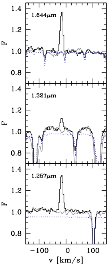
Figure 1: [FeII] emission lines (solid histogram) towards HD 200775 at $1.644$ $\mu$m (upper panel), $1.321$ $\mu$m (middle panel) and $1.257$ $\mu$m (bottom panel). The solid gray line shows the spectrum of the telluric star Hip 89584 around the [FeII] lines, while the dotted blue line outlines the telluric transmission obtained by an atmospheric model with a spectral resolution R=100000. All fluxes are plotted as a function of radial velocity $V$, assuming $V=0$ for a line emitted at the systemic velocity, and are normalized to the continuum.

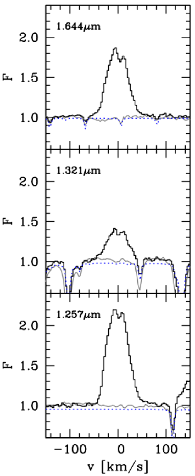
Figure 2: Same as Fig. 1, but for V1478 Cyg.

3 Intercalibration of line fluxes

Accurate line ratio derivation needs accurate flux or line ratio calibration. In principle this can be obtained either from the source spectra themselves, if known, or by observing stars during the night whose NIR spectra are known with accuracy (spectrophotometric standards). Basically, if the underlying target continuum is used, the calibrated flux is given by:

$$F_{{\rm cal},\lambda}=F_{{\rm meas},\lambda}\times\frac{A\lambda^{\alpha}}{C_{\lambda}}$$ (1)

where $F_{{\rm meas},\lambda}$ is the measured line integrated flux (in counts times wavelength), $C_{\lambda}$ is the measured continuum flux (in counts) outside the line, and $A\lambda^{\alpha}$ is the source continuum flux density (i. e., ${\rm d}F/{\rm d}\lambda$) from a fit, e. g., to the 2MASS photometry.

One problem of using the target continuum is a possible spectral variability of our sources, in addition there are no observations of spectrophotometric standards available during the night, either. However, we note that, as far as line ratios are requested, what is actually needed is an intercalibration between different wavelength ranges rather than flux calibration, which is less demanding. This can be achieved by using spectra of telluric standard stars and/or stars of known spectra which do not exhibit variability. In practice, the measured line ratio $F_{\rm meas}(\lambda_{1})/F_{\rm meas}(\lambda_{2})$, where $F_{\rm meas}(\lambda)$ is the integrated line flux (in counts by wavelength), can be calibrated multiplying it by a line-ratio calibration factor given by:

$$X=\frac{F_{\rm meas,s}(\lambda_{2})}{F_{\rm meas,s}(\lambda_{1})}\frac{S_{\rm s}(\lambda_{1})}{S_{\rm s}(\lambda_{2})}$$ (2)

where $F_{\rm meas,s}(\lambda)$ is the flux measured at $\lambda$ (in counts) from the continuum of a star of known spectrum and $S_{\rm s}(\lambda)$ is its theoretical continuum flux density at $\lambda$. This method has the advantage that the effects of changes of seeing and air mass between target and calibrator integrations mostly cancel out in the ratio.

Unfortunately, only the three targets were observed during the night of 30. Nevertheless, a few suitable sources were observed on the nights before and after. This should not be of major concern, since one can expect that, as a first approximation, continuum telluric absorption only depends on the atmospheric gas column density. Thus, line-ratio calibration factors should remain almost constant in time, at least on nearby nights. What is bound to exhibit changes is the absorption in the narrow wavelength regions dominated by telluric absorption lines. Therefore, normalized flux ratios obtained from stars of known spectra can be used as correcting factors for calibrating line ratios in the target spectra, as long as the emission lines of interest do not overlap strong telluric absorption lines.

We have checked the consistency of line-ratio calibration factors in time by using spectra of a telluric standard star, namely Hip 89584 (catalog ) (an O6.5 V star), of VEGA (catalog ) (A0 V, two observations 5 hr apart), of HD 188001 (catalog ) (O7 Iabf), and of HD 190429A (catalog ) (O4 If) taken on the night of 29 July, plus two spectra of VEGA (7 hrs apart) taken on the night of 31 July. These were reduced using the same procedure as that used for the targets. As discussed in Appendix B, we found that the calibration factors exhibit only small variations throughout the nights of 29 and 31, supporting our view that similar values can be applied to the spectra taken on 30. Therefore, the line ratios were calibrated using the mean factors derived from Hip 89584, HD 188001, and HD 190429A, listed in Table 5 in Appendix B. The values from VEGA, although consistent with the others, were not included since its observations were actually pointing tests. We estimate that the calibration uncertainty on the relevant line ratios is of order of 5-10 %.

Table 1: Integrated fluxes of the [FeII] emission lines from the stars HD 200775 and V1478 Cyg, at $1.644$, $1.321$, and $1.257$ $\mu$m, normalized to that at $1.644$ $\mu$m. Also listed: the line equivalent width, full width at half maximum, and central velocity with respect to the systemic velocity, and the extinction from the literature.

Object	$A_{V}$	$\lambda_{c}$	Int. Flux	Eq. width	$FWHM$	$v_{r}$
		($\mu$m)		(nm)	(km s-1)	(km s-1)
HD 200775	$1.8$–3(a)	1.64389	1	$-0.032$	10.76	-16.68
		1.32082	$0.32\pm 0.03$	$-0.006$	8.48	-16.82
		1.25694	$1.14\pm 0.06$	$-0.019$	11.18	-16.42
V1478 Cyg	10–10.7(b)	1.64392	1	$-0.219$	46.81	-1.03
		1.32084	$0.26\pm 0.01$	$-0.074$	48.02	-1.37
		1.25696	$0.86\pm 0.02$	$-0.265$	48.52	-0.50

4 Correction of absorption from telluric lines

Correction of absorption from telluric lines overlapping the emission lines is as critical as a good intercalibration to obtaining accurate line ratios. As shown in Sect. 5, a systematic error of 10 % in the integrated line flux is enough to cause an error of $\sim 1$ mag in the extinction. In this section we compare the uncertainty inherent telluric correction in both low- and medium- or high-resolution spectra. High-resolution spectra have the advantage of allowing an accurate mapping of the telluric lines, e. g. through spectra of telluric standard stars.

As far as our GIANO spectra are concerned, any correction for atmospheric absorption lines relies on the spectrum of the telluric standard Hip 89584, which was taken on the previous night, and simulations with the ESO Cerro Paranal Advanced Sky Model (Noll et al., 2012, hereafter ASM), which is based on the HITRAN database (Rothman et al., 2009). The spectra displayed in Figs. 1 and 2 demonstrate that all telluric features in the Hip 89584 spectrum are retrieved by ASM, so that we can safely assume that the location of the telluric absorption lines is well known and can be obtained through this code in the narrow spectral windows we are studying.

Figures 1 and 2 clearly show how much telluric absorption lines can affect the integrated flux measurements, as well. The emission lines at both $1.644$ and $1.321$ $\mu$m encompass telluric absorption lines; if this is not properly taken into account, the integrated flux will be underestimated. The middle panel of Fig. 1, shows that the $1.321$ $\mu$m line coincides with a faint atmospheric absorption line. This line is very faint: measurements on the ASM models and on the telluric star spectrum point to a change in transparency of only 1–4 %. Yet, because what is actually measured is the absorbed line plus continuum integrated flux minus the unabsorbed continuum flux density (outside the line) by the line width, this enhances the line flux lost. It can easily be seen that the systematic error in the measured integrated flux, $\Delta f_{\rm meas}$, is given by:

$$\frac{\Delta f_{\rm meas}}{f_{\rm meas}}\sim\frac{\Delta f}{f}+C\times(1-T\frac{\Delta\lambda_{\rm abs}}{\Delta\lambda_{\rm line}})$$ (3)

where $f$ is the actual emission line integrated flux, $\Delta f$ the line integrated flux absorbed, $C$ is the ratio of continuum flux density to line peak flux density, $T$ is the minimum transparency inside the telluric line, $\Delta\lambda_{\rm abs}$ is the width of the absorption line, and $\Delta\lambda_{\rm line}$ the width of the emission line. From Fig. 1 the emission line peak is less than $1/10$ of the continuum (i.e. $C\sim 10$). Thus, the equation above shows that the line integrated flux may be underestimated by more than 10 % if $\Delta\lambda_{\rm abs}\sim\Delta\lambda_{\rm line}$. The same problem of course affects the $1.321$ $\mu$m line towards V1478 Cyg, but in this case the line peak is $\sim 1/2.5$ times the continuum and the emission line is much broader, so the underestimate in integrated flux is negligible. Note that this effect increases with increasing $C$. On the other hand, pure line emission spectra ($C=0$), like in Herbig-Haro objects, are much less affected.

Methods to correct medium- and high-resolution NIR spectra for telluric line absorption are described, e. g., in Kausch et al. (2015). We used a correction scheme similar to that performed by the STSDAS routine TELLURIC, which is based on the Beer’s law, exploiting the telluric standard star spectrum. This was applied to the $1.644$ and $1.321$ $\mu$m [FeII] lines and we estimate that the effect of telluric line absorption is reduced to a few percent of the measured integrated line flux in the $1.321$ $\mu$m line after correction. The [FeII] line fluxes, normalized to the $1.644$ $\mu$m line and corrected for telluric absorption, are given in Table 1.

We point out now one possible problem with telluric absorption correction in low-resolution spectra. Using ASM, we have simulated the atmospheric absorption in three spectral windows centered at the [FeII] line rest wavelengths (see Fig. 3). The wavelengths have been converted into radial velocities and the spectral windows span an interval ranging from $-500$ to $500$ km s^-1, which should be large enough for most galactic observations of jets from YSOs and young stars. We have overplotted a high resolution ($R=50000$) spectrum, a medium resolution ($R=10000$) one, and two low resolution ones ($R=1000$ and $R=1500$). The atmospheric transmission has been estimated by assuming airmass $1.3$ and average standard values for the remaining parameters. Wider spectral intervals with the high-resolution telluric absorption spectra as a function of wavelength are displayed in Appendix C, Figs. 4, 5, and 6. One has to keep in mind that Herbig Haro and jet feature spectra are pure line spectra, therefore emission lines falling between telluric absorption lines remain unaffected by them although they are widened by the spectrograph instrumental profile at low resolution. Thus, they must be corrected using the transmission values outside the telluric lines. But one cannot achieve this by using continuum spectra of telluric standard stars. This because a correcting function is usually obtained by dividing the observed standard spectrum by a synthetic stellar spectrum. However, the observed spectrum is not just a transmission function of wavelength multiplied by a stellar spectrum, it is also convolved by an instrumental function. Since the transmission function can be roughly described as a smooth continuum component plus a number of narrow absorption lines, if the instrumental function is broad as in low resolution spectra, the convolution product in a point is affected by nearby absorption lines and results in a stronger absorption between telluric lines.

If the target exhibits a pure emission line spectrum with no or faint underlying continuum, and the emission line of interest lies outside any deep telluric line, the observed line profile is just the product of the intrinsic line profile and the smooth continuum absorption component convolved by the instrumental function. Absorption lines are of no consequence at all in this case. They do not enter in any way and the effective smooth absorption is not enhanced as is the case of a star spectrum. The effect can be roughly evaluated by looking at the middle panel of Fig. 3; the smoothing of the telluric absorption lines due to the low spectral resolution produces a pseudo-continuum with a lower transmission, $T^{\prime}(\lambda)$, than the actual one, $T(\lambda)$, in the regions between absorption lines. So, if the $1.321$ $\mu$m line falls between telluric absorption lines, it will be systematically overcorrected (by a factor $T/T^{\prime}$) by using the telluric standard star technique. From Fig. 3, the overcorrection can be estimated to be $>10$ %, a value leading to a systematic underestimate of $A_{V}$ $>1$ mag, as shown by Eq. 5. But the situation is even worse, since we have identified the telluric lines as water vapor lines, hence exhibiting the most extreme variability. Towards some objects, the $1.321$ $\mu$m line may coincide with one of the telluric absorption lines, so the reverse would happen: the line flux would be undercorrected and the extinction systematically overestimated. Interestingly, Fig. 3 shows that medium resolution spectra are unaffected by the problem and in any case telluric absorption lines can easily be retrieved.

On the other hand, the $1.257$ $\mu$m line is less likely to have similar problems. Only if it coincides with one of the two O₂ lines of the ${}^{1}\Delta_{g}$ band (which is centered at $1.27$ $\mu$m) shown in the bottom panel of Fig. 3, $A_{V}$ will result underestimated. As a consequence, the $1.257$ $\mu$m line is much more suitable for deriving $A_{V}$ from low resolution spectra. The upper panel of Fig. 3 indicates that the $1.644$ $\mu$m line, as well, is bound to be slightly overcorrected most of the times because of the absorption from lines of the 2$\nu_{3}$ band of CH₄ (which is centered at $1.66$ $\mu$m) and of CO₂. In some extreme cases it may coincide with one of the two deeper lines and underestimate the extinction. This would roughly affect the extinction from the two line ratios in the same way.

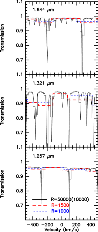
Figure 3: Atmospheric transmission model around the [FeII] emission features at $1.644$ $\mu$m (upper panel), $1.321$ $\mu$m (middle panel) and $1.257$ $\mu$m (bottom panel). The solid black line is a model computed with a spectral resolution R=50000, the black histogram one computed with R=10000, the dashed red line one computed with R=1500 and the blue dotted line one computed with R=1000. The absorption lines in the upper panel are CH₄ and CO₂ (the faintest ones), those in the middle panel are H₂O, and those in the bottom panel are O₂.

Absorption from overlapping telluric lines is therefore a non-negligible source of systematic errors in measuring NIR line ratios both from low- and high-resolution spectra. However, low-resolution emission-line spectra cannot be corrected to high precision in regions with a high number of atmospheric lines, like around $1.321$ $\mu$m, whereas high-resolution spectra allow mapping the location of telluric lines with respect to the emission lines with high accuracy through observations of telluric standard stars or models of atmospheric transmission. In the medium- and high-resolution cases, the methods available to correct for telluric line absorption appear able to constrain the uncertainty on the integrated line fluxes within few percent, provided the overlapping telluric lines are faint enough to absorb $\lesssim 10$ % of the integrated flux. More intense absorption may be difficult to constrain below $\sim 10$ % even in high-resolution spectra.

5 Deriving extinction from [FeII] line ratios

It can easily be found that the relationship between observed and intrinsic line ratios, and extinction is the following:

$$\log{\frac{F_{\lambda_{1}}}{F_{\lambda_{2}}}}=\frac{A_{\lambda_{2}}-A_{\lambda_{1}}}{2.5}+\log{\frac{I_{\lambda_{1}}}{I_{\lambda_{2}}}}$$ (4)

where $F_{\lambda_{1}},F_{\lambda_{2}}$ are the observed line fluxes, $I_{\lambda_{1}},I_{\lambda_{2}}$ are the intrinsic line fluxes, and $A_{\lambda_{1}},A_{\lambda_{2}}$ are the extinction values (in magnitudes) at wavelengths $\lambda_{1}$ and $\lambda_{2}$, respectively. If the lines originate from the same upper level, like [FeII] $1.644$, $1.321$, and $1.257$ ${\mu}$m, then in the optically thin case the ratio of intrinsic line fluxes is simply given by the ratio of the corresponding spontaneous emission coefficients, which is constant and in principle known, multiplied by the ratio of line central frequencies. $A_{\lambda_{1}}andA_{\lambda_{2}}$ can be expressed in terms of $A_{V}$ by adopting an extinction law $A_{\lambda}/A_{V}$, where $A_{V}$ is the extinction in the photometric $V$ band. Thus, Eq. 4 can be rewritten as:

$$A_{V}=\left[2.5/\left(\frac{A_{\lambda_{2}}-A_{\lambda_{1}}}{A_{V}}\right)\right]\times\left(\log{\frac{F_{\lambda_{1}}}{F_{\lambda_{2}}}}-\log{\frac{I_{\lambda_{1}}}{I_{\lambda_{2}}}}\right).$$ (5)

Values of $2.5/(A_{\lambda_{2}}-A_{\lambda_{1}})/A_{V}$ are listed in Table 2 for a few different extinction laws. Table 3 lists a few determinations of the intrinsic line ratios (see also the discussion in Sect. 6). From Eq. 5 the effect of systematic errors $\Delta F_{\lambda}$ on the measured fluxes is easily computed. This amounts to:

$$\Delta A_{V}=\left[2.5/\left(\frac{A_{\lambda_{2}}-A_{\lambda_{1}}}{A_{V}}\right)\right]\times$$

$$\left[\log\left({1+\frac{\Delta F_{\lambda_{1}}}{F_{\lambda_{1}}}}\right)-\log\left({1+\frac{\Delta F_{\lambda_{2}}}{F_{\lambda_{2}}}}\right)\right]$$ (6)

E. g., by using the extinction law of Fitzpatrick (1999) for $R_{V}=3.1$ (see Table 2) and assuming $\Delta F_{\lambda_{1}}=0$ one obtains $\Delta A_{V}\sim-1.2,-1.5$ for $\Delta F_{\lambda_{2}}/F_{\lambda_{2}}\sim 0.1$, $\lambda_{1}\sim 1.644$ $\mu$m and $\lambda_{2}\sim 1.257,1.321$ $\mu$m, and $\Delta A_{V}\sim 1.2,1.5$ for $\Delta F_{\lambda_{2}}/F_{\lambda_{2}}\sim-0.1$, $\lambda_{1}\sim 1.644$ $\mu$m and $\lambda_{2}\sim 1.257,1.321$ $\mu$m. The same figures are obtained for a systematic error $\Delta X/X\sim\pm 0.1$ on the line ratio calibration factor $X$, provided that $\Delta F_{\lambda_{2}}/F_{\lambda_{2}}$ is set equal to 0 and $\Delta F_{\lambda_{1}}/F_{\lambda_{1}}$ is replaced by $\Delta X/X$. This shows that the accuracy of the extinction derived is extremely sensitive to that of the measured line fluxes or line ratios.

Table 2: $2.5/(\frac{A_{\lambda_{2}}-A_{\lambda_{1}}}{A_{V}})$ for different extinction laws and $\lambda_{1}=1.644$ $\mu$m.

	$R_{V}=3.1$		$R_{V}=5.0$
Ext. law	$\lambda_{2}=1.257$ $\mu$m	$\lambda_{2}=1.321$ $\mu$m	$\lambda_{2}=1.257$ $\mu$m	$\lambda_{2}=1.321$ $\mu$m
RL85	23.70	30.46
CCM89	25.48	32.59	21.99	28.12
F99	28.70	37.26	27.65	36.55

The intrinsic error $\sigma F_{\lambda}$ on the measured flux $F_{\lambda}$ propagates to give the following error on the derived extinction:

$$\sigma A_{V}=0.43\times\left[2.5/\left(\frac{A_{\lambda_{2}}-A_{\lambda_{1}}}{A_{V}}\right)\right]\times$$

$$\sqrt{\left(\frac{\sigma F_{\lambda_{1}}}{F_{\lambda_{1}}}\right)^{2}+\left(\frac{\sigma F_{\lambda_{2}}}{F_{\lambda_{2}}}\right)^{2}}$$ (7)

From Table 1 and in the same assumptions as above, it can be easily found a range $\sigma A_{V}\sim 0.6-1.5$, which are comparable with the systematic errors due to calibration.

6 Discussion

The purpose of this section is applying the relations provided in the previous section to our measured Fe⁺ line ratios, deriving a set of extinction values, and comparing them with those found in the literature. This is a purely didactic exercise, since the extinction given in the literature for our targets is a photospheric extinction, whereas the Fe⁺ is likely to arise in outermost, less reddened regions. The extinction determination to our targets is widely discussed in Hernández et al. (2004) (HD200775) and Cohen et al. (1985) (V1478 Cyg). As for HD200775, Hernández et al. (2004) compare optical colors and intrinsic colors (from the star spectral type) obtaining $A_{V}$ in the range $1.8-3$ mag, which appears quite robust. Cohen et al. (1985) discuss a few diagnostics for V1478 Cyg, all pointing to an extinction $A_{V}$ in the range $10-10.7$ mag; values as low as $A_{V}=8$ seems unlikely. Although these photospheric extinction values can only provide an upper limit to the values yielded by [FeII] line ratios, a comparison is quite a useful exercise for highlighting the different results from the available Einstein coefficient computations and the effects from the various sources of errors.

We derived the extinction to the stars HD 200775 and V1478 Cyg out of the two line ratios $1.644/1.257$ and $1.644/1.321$, from Eq. 5. We used the measured line ratios given in Table 1 and the intrinsic line ratios of Nussbaumer & Storey (1988), as in Nisini et al. (2005), the empirical determinations of Giannini et al. (2015a), and the values discussed in Bautista et al. (2015), including their recommended values. We tested the effect of changing the extinction law by using the relation given by Draine (1989), that of Rieke & Lebofsky (1985) as in Nisini et al. (2005), and that of Fitzpatrick (1999) for $R_{V}=5.0$. Hernández et al. (2004) found that most HAe/Be stars in their sample exhibit a reddening better characterized by $R_{V}=5.0$; the extinction curves of Fitzpatrick (1999) allow us to investigate the effect of changing $R_{V}$. The results are listed in Table 4. We note that only the errors due to the measured fluxes have been taken into account. Systematic errors in the calibration coefficients (which we have estimated $\sim 5-10$ %) may induce shifts of $\sim 0.5-1.5$ mag (at most).

We rule out the Einstein coefficients which lead to extinctions more than one sigma either below zero or above the $A_{V}$ values quoted in Table 1 for at least one of the two stars. Namely, the ones labeled BPeTFDAc and Q96 (Bautista et al., 2015). That labeled SST can probably be discarded, as well. The upper limits of Giannini et al. (2015a) give a systematically lower extinction compared with the other theoretical values, therefore we tentatively exclude them from our analysis. The remaining sets of Einstein coefficients lead to $A_{V}$ in the range $0.3-3.6$ mag for HD 200775, which agree with the range $1.8-3$ mag given in Table 1, and in the range $2.5-6.9$ mag for V1478 Cyg, below the values $10-10.7$ mag given in Table 1, all systematically lower. The two line ratios always yield reddening values consistent with each other within errors. The differences caused by changing the extinction law adopted become important at high reddening.

However, if we restrict our analysis to the most likely values of the Einstein coefficients, e. g. the recommended set of Bautista et al. (2015), the lower limits of Giannini et al. (2015a), and the computation by Nussbaumer & Storey (1988), we find $A_{V}\sim 1-2$ mag ($R_{V}=5$) for HD 200775, and $A_{V}\sim 2.5-5$ for V1478 Cyg. These are systematically lower than the extinctions given in Table 1 (note that $A_{V}\sim 3$ for HD 200775 when assuming $R_{V}=5$, as recommended by Hernández et al. (2004)). The intrinsic line ratios entering Eq. 5 are listed in Table 3 for the three sets of Einstein coefficients and in the case of optically thick emission (blackbody at 3000, 5000, 10000, 15000, and 20000 K), as well. By comparing Eq. 5 and Table 3 it is easily seen that optically thick emission would yield highly discrepant values of $A_{V}$ from the two line ratios, shifting them in opposite directions by a few magnitudes, confirming that the line intensities are in the optically thin case for both stars.

Table 3: Intrinsic line ratios ($\frac{I_{\lambda_{1}}}{I_{\lambda_{2}}}$ in Eq. 5) from the most recent values of the Einstein coefficients, with $\lambda_{1}=1.644$ $\mu$m. Also listed, values in the optically thick case.

Source	$\lambda_{2}=1.257$ $\mu$m	$\lambda_{2}=1.321$ $\mu$m
Rec	0.80	2.91
Gia15min	0.83	3.03
NS88	0.96	3.45
Opt. thick A	1.50	1.42
Opt. thick B	2.05	1.81
Opt. thick C	2.50	2.12
Opt. thick D	2.65	2.22
Opt. thick E	2.72	2.26

Table 4: $A_{V}$ as a function of the adopted Einstein coefficients (first column) for HD 200775 and V1478 Cyg. $A_{V}^{a}$ and $A_{V}^{b}$ are computed from the $1.644/1.257$ and $1.644/1.321$ line ratios, respectively.

HD 200775	$A_{V,D}^{a}$	$A_{V,D}^{b}$	$A_{V,F}^{a}$	$A_{V,F}^{b}$	$A_{V,R}^{a}$	$A_{V,R}^{b}$
SST	$-1.0\pm 0.5$	$-2.0\pm 1.3$	$-1.1\pm 0.6$	$-2.4\pm 1.5$	$-0.9\pm 0.5$	$-1.9\pm 1.2$
HFR	$0.4\pm 0.5$	$-0.1\pm 1.3$	$-0.5\pm 0.6$	$-0.2\pm 1.5$	$0.4\pm 0.5$	$-0.1\pm 1.2$
HFRnew	$3.0\pm 0.5$	$3.1\pm 1.3$	$3.3\pm 0.6$	$3.6\pm 1.5$	$2.8\pm 0.5$	$2.9\pm 1.2$
CIV3	$1.9\pm 0.5$	$1.9\pm 1.3$	$2.1\pm 0.6$	$2.2\pm 1.5$	$1.8\pm 0.5$	$1.8\pm 1.2$
BPeTFDAc	$-5.3\pm 0.5$	$-6.4\pm 1.3$	$-6.0\pm 0.6$	$-7.4\pm 1.5$	$-5.0\pm 0.5$	$-6.0\pm 1.2$
Q96	$7.9\pm 0.5$	$10.3\pm 1.3$	$8.9\pm 0.6$	$11.9\pm 1.5$	$7.4\pm 0.5$	$9.6\pm 1.2$
7-config	$1.1\pm 0.5$	$2.3\pm 1.3$	$1.3\pm 0.6$	$2.7\pm 1.5$	$1.0\pm 0.5$	$2.2\pm 1.2$
TFDAc	$0.3\pm 0.5$	$0.5\pm 1.3$	$0.4\pm 0.6$	$0.6\pm 1.5$	$0.3\pm 0.5$	$0.5\pm 1.2$
Rec	$1.0\pm 0.5$	$1.1\pm 1.3$	$1.1\pm 0.6$	$1.3\pm 1.5$	$0.9\pm 0.5$	$1.0\pm 1.2$
Gia15max	$-0.4\pm 0.5$	$-0.2\pm 1.3$	$-0.4\pm 0.6$	$-0.3\pm 1.5$	$-0.3\pm 0.5$	$-0.2\pm 1.2$
Gia15min	$0.6\pm 0.5$	$0.8\pm 1.3$	$0.7\pm 0.6$	$1.0\pm 1.5$	$0.6\pm 0.5$	$0.8\pm 1.2$
NS88	$2.0\pm 0.5$	$1.6\pm 1.3$	$2.2\pm 0.6$	$1.9\pm 1.5$	$1.9\pm 0.5$	$1.5\pm 1.2$
V1478 Cyg	$A_{V,D}^{a}$	$A_{V,D}^{b}$	$A_{V,F}^{a}$	$A_{V,F}^{b}$	$A_{V,R}^{a}$	$A_{V,R}^{b}$
SST	$2.0\pm 0.2$	$0.8\pm 0.8$	$2.2\pm 0.2$	$0.9\pm 0.9$	$1.8\pm 0.2$	$0.7\pm 0.7$
HFR	$3.4\pm 0.2$	$2.7\pm 0.8$	$3.8\pm 0.2$	$3.2\pm 0.9$	$3.2\pm 0.2$	$2.5\pm 0.7$
HFRnew	$5.9\pm 0.2$	$6.0\pm 0.8$	$6.7\pm 0.2$	$6.9\pm 0.9$	$5.5\pm 0.2$	$5.6\pm 0.7$
CIV3	$4.9\pm 0.2$	$4.8\pm 0.8$	$5.5\pm 0.2$	$5.5\pm 0.9$	$4.5\pm 0.2$	$4.6\pm 0.7$
BPeTFDAc	$-2.4\pm 0.2$	$-3.6\pm 0.8$	$-2.7\pm 0.2$	$-4.1\pm 0.9$	$-2.2\pm 0.2$	$-3.3\pm 0.7$
Q96	$10.9\pm 0.2$	$13.1\pm 0.8$	$12.3\pm 0.2$	$15.2\pm 0.9$	$10.2\pm 0.2$	$12.2\pm 0.7$
7-config	$4.1\pm 0.2$	$5.1\pm 0.8$	$4.6\pm 0.2$	$6.0\pm 0.9$	$3.8\pm 0.2$	$4.8\pm 0.7$
TFDAc	$3.3\pm 0.2$	$3.3\pm 0.8$	$3.7\pm 0.2$	$3.9\pm 0.9$	$3.1\pm 0.2$	$3.1\pm 0.7$
Rec	$4.0\pm 0.2$	$3.9\pm 0.8$	$4.5\pm 0.2$	$4.6\pm 0.9$	$3.7\pm 0.2$	$3.7\pm 0.7$
Gia15max	$2.6\pm 0.2$	$2.6\pm 0.8$	$2.9\pm 0.2$	$3.0\pm 0.9$	$2.4\pm 0.2$	$2.4\pm 0.7$
Gia15min	$3.6\pm 0.2$	$3.7\pm 0.8$	$4.0\pm 0.2$	$4.2\pm 0.9$	$3.3\pm 0.2$	$3.4\pm 0.7$
NS88	$5.0\pm 0.2$	$4.4\pm 0.8$	$5.6\pm 0.2$	$5.2\pm 0.9$	$4.6\pm 0.2$	$4.2\pm 0.7$

On the other hand, most of the Einstein coefficients yielding extinctions inside the range limited by the photospheric value also lead to extinctions which differ at most by $\sim 2.5$ mag. In particular, the Einstein coefficients recommended by Bautista et al. (2015) result in extinctions quite similar as those obtained from the lower limits of Giannini et al. (2015a) through observations. This points to the latest determinations leading to uncertainties not larger than $\sim 1$ mag.

It is interesting to investigate the discrepancies reported in the literature between $A_{V}$ as determined from the two line ratios. Nisini et al. (2005) found that the extinction towards HH1 estimated from the $1.644/1.257$ ratio is a factor $\sim 2$ systematically larger than that estimated from the $1.644/1.321$ ratio when using the Einstein coefficients of Nussbaumer & Storey (1988) and low spectral resolution data. On the one hand, we note from Table 4 that the extinction obtained using the Einstein coefficients of Bautista et al. (2015) (or the lower limit of Giannini et al. (2015a)) is $\sim 1-2$ mag lower than that obtained using the Einstein coefficients of Nussbaumer & Storey (1988), which mostly removes the discrepancy pointed out by Nisini et al. (2005) on the $1.644/1.257$ ratio vs. optical determination. On the other hand, the difference in extinction of the two ratios obtained using the Einstein coefficients of Nussbaumer & Storey (1988) is $\sim 0.5$ mag, but nonetheless within the errors propagated from the signal to noise ratios of the single lines.

Analogously, Giannini et al. (2015a) found intrinsic ratios $I(1.321\mu{\rm m})/I(1.644\mu{\rm m})$ larger than expected from a few literature observations of jet features (see their Fig. 3). We note that these, as well, are mostly data from low spectral resolution spectra (SofI and ISAAC). Low resolution spectra appear unsuitable for deriving accurate extinction or the Einstein coefficients of the [FeII] lines due to the insufficient correction of the atmospheric absorption achievable (see Sect. 4). In this case we recommend that the extinction be derived from the $1.644/1.257$ ratio rather than the $1.644/1.321$, i. e. the one less affected by telluric absorption lines.

7 Conclusions

We have reviewed the commonly used technique of deriving extinction to young stellar objects through [FeII] line ratios $1.644/1.257$ $\mu$m and $1.644/1.321$ $\mu$m, all lines arising from the same upper level. In particular, we have provided the relevant equations, discussed all the main sources of systematic errors, and roughly tested the most recent determinations of the Einstein coefficients available in the literature. We have checked the method by attempting to derive the extinction of a Herbig Be star (HD 200775) and a Be star (V1478 Cyg) from high ($R\sim 50000$) resolution spectra obtained with the GIANO spectrometer. High resolution spectra are particularly suitable for a direct assessment of the effect of telluric absorption. In addition, the broad band of GIANO allows simultaneous acquisition at all relevant wavelengths, making line-ratio calibration easier.

Although we have shown that the most recent determinations of the Einstein coefficients (e. g., the recommended values of Bautista et al. (2015)) are probably accurate enough to derive $A_{V}$ to within 1 mag of error, we found that both the calibration and the telluric absorption correction is critical. In addition, we have shown that a $>10$ % error in the line integrated fluxes measured is enough to produce a $>1$ mag error in $A_{V}$. So, an accurate determination of reddening requires high-signal-to-noise line fluxes. The most accurate extinction values we are able to provide for our targets are $A_{V}=1.1\pm 0.6$ for the Herbig B star HD 200775, to compare with $A_{V}\sim 3$ found in the literature, and $A_{V}=3.7\pm 0.2$ for V1478 Cyg, to compare with $A_{V}\sim 10$ found in the literature. This discrepancy arises from the fact that [FeII] lines originate from less extincted regions than the central stars.

We have also discussed the problems affecting low resolution ($R\sim 1000-1500$) spectra and shown that the commonly adopted technique of correcting the telluric absorption by exploiting continuum spectra of standard stars can induce significant calibration errors in emission line-only spectra (Herbig Haro objects, jets from young stellar objects). In particular, the $1.321$ $\mu$m line falls in a spectral window characterized by deep absorption lines of H₂O, so its flux is prone to be overestimated, but could also be heavily underestimated in extreme cases. If low resolution spectra of [FeII] are used to derive $A_{V}$, we advice that this should be derived from the $1.644/1.257$ ratio only, which is less likely to be significantly affected by the telluric absorption correction. Medium resolution spectra ($R\sim 10000$) appear unaffected by the problem and in any case telluric absorption lines are easily retrieved at this resolution.

Both the determination of $A_{V}$ and the empirical determination of the Einstein coefficients from NIR [FeII] lines should be done exploiting high resolution spectra, taking particular care to calibrate and correct the spectra for telluric absorption.

Finally, we note that the problem of the telluric correction of NIR low resolution spectra using standard stars can affect ratios from a large number of different lines, as well. Therefore, we advice that telluric absorption simulations (e. g., with the ESO ASM) be performed case by case to investigate the issue.

Appendix A Data reduction

All spectral orders obtained through a GIANO exposure are output in a single image. To reduce these 2D spectra, extract the one-dimensional (1D) spectra, and wavelength-calibrate them, we used the ECHELLE package in IRAF and some ad-hoc scripts gathered in the GIANO_TOOLS package. Note that a GIANO image actually contains two spectra (one per optical fiber). Each fiber output is also split in two different light sources over the slit by using an image slicer, so each order on the 2D subtracted image is composed of 4 close-by parallel tracks, two per fiber (see, e. g., Fig. 1 of Origlia et al. (2013)). The spectra were flat-fielded by using exposures on a continuum reference lamp and bad-pixel corrected. A polynomial was fit to the peak positions of each (high signal-to-noise) track of the continuum-lamp reference spectrum. The 1D target spectra were extracted from the 2D images by summing 4 pixels around the loci defined by the polynomials, in the direction perpendicular to the dispersion. For wavelength calibration we took spectra of a reference U-Ne lamp. The resulting wavelength accuracy is better than $0.01$ nm (see http://www.bo.astro.it/giano/documents/), i. e., better than $1.5-3$ km s^-1 (we note that the achieved spectral resolution amounts to $\sim 6$ km s^-1). Finally, all four 1D spectra per order extracted from each A$-$B image were summed together to improve the signal-to-noise ratio. Wavelengths were converted into radial velocities in the spectral regions around the [FeII] lines and the radial velocities were referred to the systemic velocity so that the rest (laboratory) wavelength of each line lies at zero velocity. This allows one to visually identify radial motions (outflows, inflows) with respect to the parent star when plotting the spectra as a function of radial velocity. We searched the literature for the star radial velocities either in the heliocentric or in the local standard of rest. HD 200775 is a binary system with members of similar mass, so we used the relation of Alecian et al. (2008) to correct velocities to the heliocentric standard. The hydrogen emission lines appear roughly centered at 0 km s^-1 in the rest frame of the secondary star, whereas they are slightly red-shifted in the rest frame of the primary one. This favors the less massive member as the Herbig Be star of the pair, in contrast to Benisty et al. (2013), who associated the Herbig Be star with the more massive member. As for V1478 Cyg, radial velocities in the local standard of rest are from Gordon et al. (2001).

Appendix B Notes on line flux ratio calibration

In principle, one can correct the 1D spectra for instrumental sensitivity and continuum atmospheric absorption by using $J,H,K$ photometry of the targets themselves from the 2MASS Point Source Catalog. In a simple case, assuming that the source continuum spectra are well approximated by power laws, $J,H,K$ fluxes are fit by a $F_{\lambda}=A\lambda^{\alpha}$ law, where $A$ and $\alpha$ are free parameters. Then, one can use a linear least-square in logarithmic form and calibrate the flux density for each line through Eq. 1, by measuring the continuum level (in counts) in narrow spectral intervals adjacent to the lines. Although this entails a systematic error in line fluxes if continuum- and line-emitting regions are not spatially coincident, line ratios are unaffected as long as a correction for absorption from overlapping telluric lines is also applied where needed (see Sect. 4).

However, one has to keep in mind that Herbig Ae/Be stars are typically variable in flux. So, if their NIR spectral slopes change as well, deriving $A,\alpha$ from the 2MASS photometry (carried out long before our observations) is not adequate to calibrate our targets. An error in the spectral slope enters the calibration with large effects, causing systematic errors in $A_{V}$. By combining Eq. 5 and Eq. 1, and approximating the calibration error to a systematic error $\Delta\alpha$ on the exponent of the calibrating continuum flux, one obtains:

$$\Delta A_{V}=\Delta\alpha\times 2.5\log{(\frac{\lambda_{1}}{\lambda_{2}})}/[(A_{\lambda_{2}}-A_{\lambda_{1}})/A_{V}].$$ (B1)

Using the extinction law of Fitzpatrick (1999) for $R_{V}=3.1$, one obtains:

$$\Delta A_{V}=3.54\times\Delta\alpha$$ (B2)

from the $1.644/1.321$ ratio and

$$\Delta A_{V}=3.35\times\Delta\alpha$$ (B3)

from the $1.644/1.257$ ratio. The extinction obtained from Eq. 5 is then quite sensitive to calibration errors, as well.

In fact, V1478 Cyg is known to be highly variable in the optical ($\sim 2$ mag in $B$ and $\sim 1$ mag in $R$, Gvaramadze & Menten (2012), whereas HD 200775 exhibits either no significant variations in $B$ and $V$ (Halbedel, 1989) or of just a few hundredth of a magnitude in the optical (Sudzius & Sperauskas 1996).

As explained in Sect. 3, direct calibration of line ratios using reference spectra of stars of known continuum is easier and allows circumventing many problems. The basic relation is given by Eq. 2. Since no observations of standard stars of known spectra were performed on the night of July 30, a basic step is checking that the normalized line ratios from the star spectra taken on the nights of July 29 and 31 do not exhibit significant changes. If so, one can assume that the continuum atmospheric absorption between telluric lines mostly depends on the air column density and that seeing variations affect the fraction of light fed into the fibers almost independently on wavelengths. We have checked the variations of $X$ (as defined in Eq. 2) in time by using the spectra of the stars listed in Sect. 3 The line-ratio calibration factors obtained from these stars are listed in Table 5, along with those obtained from the target continuum spectra by using their 2MASS photometry. Table 5 also includes calibration factors for ratios $2.14/1.25$ $\mu$m and $2.14/1.70$ $\mu$m, wavelength intervals selected for being devoid of telluric absorption lines. For Hip 89584, we also derived the line-ratio calibration factors by using a blackbody to compute a scaled continuum flux. We adopted a blackbody temperature of 42280 K, the effective temperature of an O6.5 V star according to Vacca, Garmany & Shull (1996). The spectrum was shifted in wavelength to account for the source radial velocity of $-53$ km s^-1. By comparing the source NIR colors from the 2MASS Point Source Catalog and those of an unreddened O6.5 V star as given by Koornneef (1983) and using the extinction law of Fitzpatrick (1999) for $R_{V}=3.1$, we obtained $A_{V}\sim 1.97$. The blackbody spectrum was then reddened by this amount, as well. We found that the line-ratio calibration factors obtained for Hip 89584 using the reddened blackbody are within $1.5$ % of those derived by simply using a fit to the 2MASS NIR fluxes. Therefore, we only used the latter method in deriving the correction coefficients, which should be accurate enough at least for the O stars.

Table 5: Line-ratio calibration factors for selected line wavelength ratios. Also listed, those obtained from the targets by using their 2MASS fluxes.

Target	Calibrator	Date and time	$1.644/1.257$	$1.644/1.321$	$2.14/1.25$	$2.14/1.70$
		of observation
	VEGA	2013-07-29/22:14:38	$0.274$	$0.340$	$0.094$	$0.425$
	Hip 89584	2013-07-29/23:27:10	$0.278$	$0.340$	$0.100$	$0.441$
	HD 188001	2013-07-30/00:53:24	$0.269$	$0.329$	$0.090$	$0.417$
	HD 190429A	2013-07-30/01:06:38	$0.264$	$0.322$	$0.096$	$0.430$
	VEGA	2013-07-30/03:36:33	$0.274$	$0.342$	$0.097$	$0.422$
HD 200775		2013-07-31/03:41:41	$0.394$	$0.447$	$0.152$	$0.467$
V1686 Cyg		2013-07-31/03:50:49	$0.501$	$0.559$	$0.322$	$0.712$
V1478 Cyg		2013-07-31/04:32:31	$0.275$	$0.335$	$0.100$	$0.459$
	VEGA	2013-07-31/20:39:41	$0.269$	$0.340$	$0.086$	$0.407$
	VEGA	2013-08-01/03:20:47	$0.294$	$0.360$	$0.124$	$0.445$

Clearly, the line-ratio correction factors remained constant within at list a 10 % during the whole night of 29 for every wavelength pair. The picture gets worse on the night of 31. The line-ratio correction factors to apply to the [FeII] wavelengths, however, still remained constant within a 10 %. Furthermore, all the night mean values are within 10 % of each other. The line-ratio correction factors obtained from the 2MASS photometry of V1478 Cyg are within 10 % of the mean values of the other two nights, with those for the [FeII] wavelengths within 5 %. This suggests that its NIR spectral slope has not varied significantly. Conversely, the line-ratio correction factors obtained from the 2MASS photometry of both HD 200775 and V1686 Cyg are very different from all others, suggesting that their NIR spectral slopes have significantly changed.

The small variations exhibited by the line-ratio calibration factors for different stars throughout two nights strongly points towards confirming our assumptions of them being only weakly sensitive to weather and seeing variations on close-by nights. This should still allow us to obtain calibrated [FeII] line ratios with an accuracy within 5-10 %.

Appendix C Telluric absorption spectra in the [FeII] region

Figure 4: Atmospheric transmission around the [FeII] emission features at $1.644$ $\mu$m computed with a spectral resolution R=50000. The absorption lines are CH₄ and CO₂ (the fainter ones). The spectrum is obtained with the ESO Cerro Paranal Advanced Sky Model.

Figure 5: Atmospheric transmission around the [FeII] emission features at $1.321$ $\mu$m computed with a spectral resolution R=50000. The absorption lines are H₂O. The spectrum is obtained with the ESO Cerro Paranal Advanced Sky Model.

Figure 6: Atmospheric transmission around the [FeII] emission features at $1.257$ $\mu$m computed with a spectral resolution R=50000. The absorption lines are O₂. The spectrum is obtained with the ESO Cerro Paranal Advanced Sky Model.

References

- Alecian et al. (2008) Alecian, E., Catala, C., Wade, G. A., et al. 2008, MNRAS, 385, 391
- Bautista et al. (2015) Bautista, M. A., Fivet, V., Ballance, C., et al. 2015, ApJ, 808, 174
- Benisty et al. (2013) Benisty, M., Perraut, K., Mourard, D., et al. 2013, A&A, 555, A113
- Cardelli et al. (1989) Cardelli, J. A., Clayton, G. C., & Mathis, J. S. 1989, ApJ, 345, 245
- Cohen et al. (1985) Cohen, M., Bieging, J. H., Dreher, J. W., & Welch, W. J. 1985, ApJ, 292, 249
- Draine (1989) Draine, B. T. 1989, ESA-SP290, 93
- Fitzpatrick (1999) Fitzpatrick, E. L. 1999, PASP, 111, 63
- Giannini et al. (2013) Giannini, T., Nisini, B., Antoniucci, S., et al. 2013, ApJ, 778, 71
- Giannini et al. (2015a) Giannini, T., Antoniucci, S., Nisini, B., et al. 2015a, ApJ, 798, 33
- Giannini et al. (2015b) Giannini, T., Antoniucci, S., Nisini, B., Bacciotti, F., & Podio, L. 2015b, ApJ, 814, 52
- Gordon et al. (2001) Gordon, M. A., Holder, B. P., Jisonna, L. J., Jr., Jorgenson, R. A., & Strelnitski, V. S. 2001, ApJ, 559, 402
- Gvaramadze et al. (2012) Gvaramadze, V. V. & Menten, K. M. 2012, A&A, 541, A7
- Halbedel (1989) Halbedel, E. M. 1989, PASP, 101, 1004
- Hernández et al. (2004) Hernández, J., Calvet, N., Briceño, C., Hartmann, L., & Berlind, P. 2004, AJ, 127, 1682
- Hollenbach et al. (1989) Hollenbach, D. & McKee, C. F. 1989, ApJ, 342, 306
- Kausch et al. (2015) Kausch, W., Noll, S., Smette, A., et al. 2015, A&A, 576, A78
- Koornneef (1983) Koornneef, J. 1983, A&A, 128, 84
- Massi et al. (2008) Massi, F., Codella, C., Brand, J., di Fabrizio, L., & Wouterloot, J. G. A. 2008, A&A, 490, 1079
- Nisini et al. (2005) Nisini, B., Bacciotti, F., Giannini, T., et al. 2005, A&A, 441, 159
- Noll et al. (2012) Noll, S., Kausch, W., Barden, M., et al. 2012, A&A, 543, A92
- Nussbaumer et al. (1988) Nussbaumer, H. & Storey, P. J. 1988, A&A, 193, 327
- Origlia et al. (2013) Origlia, L., Oliva, E., Maiolino, R., et al. 2013, A&A, 560, A46
- Rieke et al. (1985) Rieke, G. H. & Lebofsky, M. J. 1985, ApJ, 288, 618
- Rothman et al. (2009) Rothman, L. S., Gordon, I. E., Barbe, A., et al. 2009, JQS&RT, 110, 533
- Sudzius et al. (1996) Sudzius, J. & Sperauskas, J. 1996, Astron. Nachr., 317, 349
- Vacca et al. (1996) Vacca, W. D., Garmany, C. D., & Shull, J. M. 1996, ApJ, 460, 914