Poincaré trace inequalities in $BV(\mathbb{B}^{n})$ with nonstandard normalization

Abstract

Extremal functions are exhibited in Poincaré trace inequalities for functions of bounded variation in the unit ball ${\mathbb{B}}^{n}$ of the $n$-dimensional Euclidean space ${{\mathbb{R}}^{n}}$. Trial functions are subject to either a vanishing mean value condition, or a vanishing median condition in the whole of ${\mathbb{B}}^{n}$, instead of just on $\partial{\mathbb{B}}^{n}$, as customary. The extremals in question take a different form, depending on the constraint imposed. In particular, under the latter constraint, unusually shaped extremal functions appear. A key step in our approach is a characterization of the sharp constant in the relevant trace inequalities in any admissible domain $\Omega\subset{{\mathbb{R}}^{n}}$, in terms of an isoperimetric inequality for subsets of $\Omega$.

1 Introduction

Let $\Omega$ be a bounded connected open set – briefly, a domain – in ${{\mathbb{R}}^{n}}$, $n\geq 2$. Under suitable regularity assumptions on its boundary $\partial\Omega$, a linear trace operator is defined on the space $BV(\Omega)$ of real-valued functions of bounded variation in $\Omega$. Such an operator maps any function $u\in BV(\Omega)$ into a function $\widetilde{u}\in L^{1}(\partial\Omega)$, the Lebesgue space of integrable functions on $\partial\Omega$ with respect to the $(n-1)$-dimensional Hausdorff measure ${\cal H}^{n-1}$. Moreover, the operator

(1.1) $$BV(\Omega)\ni u\mapsto\widetilde{u}\in L^{1}(\partial\Omega)$$

is bounded; namely, there exists a constant $C$ such that

(1.2) $$\|\widetilde{u}\|_{L^{1}(\partial\Omega)}\leq C\|u\|_{BV(\Omega)}$$

for every $u\in BV(\Omega)$. Here,

(1.3) $$\|u\|_{BV(\Omega)}=\|u\|_{L^{1}(\Omega)}+\|Du\|(\Omega),$$

the standard norm in $BV(\Omega)$, where $\|Du\|(\Omega)$ denotes the total variation in $\Omega$ of the vector-valued Radon measure $Du$.

Poincaré type inequalities also hold, with the full norm $\|u\|_{BV(\Omega)}$ replaced by just $\|Du\|(\Omega)$, provided that trial functions $u$ are normalized by an appropriate operator $BV(\Omega)\ni u\mapsto T(u)\in\mathbb{R}$. The relevant inequalities take the form

(1.4) $$\|\widetilde{u}-T(u)\|_{L^{1}(\partial\Omega)}\leq C\|Du\|(\Omega)$$

for $u\in BV(\Omega)$. A classical choice for $T(u)$ is the mean value ${\rm mv}_{\partial\Omega}(\widetilde{u})$ of $\widetilde{u}$ over $\partial\Omega$, given by ${\rm mv}_{\partial\Omega}(\widetilde{u})=\frac{1}{{\cal H}^{n-1}(\partial\Omega)}\int_{\partial\Omega}\widetilde{u}(x)\,d{\cal H}^{n-1}(x)$. Another customary option is to take $T(u)={\rm med}_{\partial\Omega}(\widetilde{u})$, the median of $\widetilde{u}$ on $\partial\Omega$, defined as ${{\rm med}}_{\partial\Omega}(\widetilde{u})=\inf\{t\in\mathbb{R}:{\cal H}^{n-1}(\{\widetilde{u}>t\})\leq{\cal H}^{n-1}(\partial\Omega)/2\}$. General assumptions on the operator $T$ for (1.4) to hold can be exhibited via a specialization of an abstract result from [Zi, Lemma 4.1.3].

In the present paper we focus on the unconventional cases when either

$$T(u)={\rm mv}_{\Omega}(u),$$

where ${\rm mv}_{\Omega}(u)=\frac{1}{|\Omega|}\int_{\Omega}u(x)\,dx$, the mean value of $u$ in $\Omega$, or

$$T(u)={\rm med}_{\Omega}(u),$$

where ${{\rm med}}_{\Omega}(u)=\inf\{t\in\mathbb{R}:|\{u>t\}|\leq|\Omega|/2\}$, the median of $u$ in $\Omega$. Here, $|\cdot|$ denotes Lebesgue measure. These choices make inequality (1.4) nonstandard, in that its left-hand side combines quantities depending both on $\widetilde{u}$ and on $u$.

We are concerned with the problem of the optimal constant $C$ in (1.4) for these two choices of $T$. Our contribution amounts to a characterization of such optimal constants in terms of geometric constants of isoperimetric type, and, primarily, to the explicit description of the extremal functions in the case when $\Omega$ is a ball. In fact, due to the scaling invariance of the relevant inequalities, we shall deal, without loss of generality, with the unit ball $\mathbb{B}^{n}$, centered at $0$, in $\mathbb{R}^{n}$.

Interestingly, the extremals in question differ substantially according to whether $T(u)={\rm mv}_{\mathbb{B}^{n}}(u)$ or $T(u)={{\rm med}}_{\mathbb{B}^{n}}(u)$. As in all known sharp Poincaré type inequalities for functions of bounded variation, in both cases extremal functions are characteristic functions of subsets $\mathbb{B}^{n}$. As far as the inequality

(1.5) $$\|\widetilde{u}-{\rm mv}_{\mathbb{B}^{n}}(u)\|_{L^{1}(\partial\mathbb{B}^{n})}\leq C\|Du\|(\mathbb{B}^{n}),$$

with an optimal constant $C$, is concerned, extremals turn out to be characteristic functions of half-balls. Hence, inequality (1.5) shares the same extremals with the more standard Poincaré trace inequality in $BV({\mathbb{B}}^{n})$ with ${\rm mv}_{\partial\mathbb{B}^{n}}$ normalization (at least for $n\geq 3$) [Ci3], and with the mean value Poincaré inequality in the whole of $\mathbb{B}^{n}$ [Ci1].
By contrast, characteristic functions of a striking kind of sets are extremals in the inequality

(1.6) $$\|\widetilde{u}-{\rm med}_{\mathbb{B}^{n}}(u)\|_{L^{1}(\partial\mathbb{B}^{n})}\leq C\|Du\|(\mathbb{B}^{n})$$

with optimal constant $C$. Unlike the case when $T(u)={{\rm med}}_{\partial\mathbb{B}^{n}}(u)$, where characteristic functions of half-balls are still extremals [BM], the extremals in (1.6) are characteristic functions of half-moon shaped subsets of $\mathbb{B}^{n}$. In particular, such extremals are not even convex. The isoperimetric nature of the optimal constant in inequality (1.6), to which we alluded above, helps in accounting for this seemingly surprising conclusion.

The geometric characterizations of the sharp constant in inequalities (1.5) and (1.6) are established in Section 2, where some definitions and basic facts from the theory of functions of bounded variation and of sets of finite perimeter are also recalled. The results of Section 2 are then exploited in Sections 3 and 4 as point of departure for the proof of sharp forms of inequalities (1.5) and (1.6), respectively. Variant inequalities, where $|\Omega|/2$ is replaced with an arbitrary fraction of $|\Omega|$ in the definition of median, or where trial functions $u$ are required to vanish on a subset of $\Omega$ of prescribed measure, are also considered in Sections 2 and 4.

We conclude this section by mentioning that trace inequalities in Sobolev type spaces, involving optimal constants, have been extensively investigated in the literature. Contributions along this line of research include [AFV, AMR, BGP, Bro, BrF, Ci2, CFNT, DDM, Es1, MV1, MV2, Ma1, Ma2, Ma3, Na, Ro, W]. Sharp forms of Poincaré type inequalities for Sobolev functions and functions of bounded variation, involving norms of $u$ in the whole of $\Omega$, are the object of [BK, BoV, BrV, Ci1, DG, DN, EFKNT, ENT, FNT, GW, Le]. In particular, the paper [NR] deals with Poincaré type inequalities for norms on $\Omega$ of functions from the Sobolev space $W^{1,2}(\Omega)$, subject to a normalization on their traces, which are, in a sense, complementary to those considered here.

2 Isoperimetric constants

Let $E$ be a measurable set in ${{\mathbb{R}}^{n}}$. The essential boundary $\partial^{M}E$ of $E$ is defined as the complement in $\mathbb{R}^{n}$ of the sets of points of densities $0$ and $1$ with respect to $E$. One has that $\partial^{M}E$ is a Borel set, and $\partial^{M}E\subset\partial E$, the topological boundary of $E$.
The set $E$ is said to be of finite perimeter relative to an open set $\Omega\subset{{\mathbb{R}}^{n}}$ if $D\chi_{E}$, the distributional derivative of the characteristic function $\chi_{E}$ of $E$, is a vector-valued Radon measure in $\Omega$ with finite total variation in $\Omega$. The perimeter of $E$ relative to $\Omega$ is defined as

(2.1) $$P(E;\Omega)=\|D\chi_{E}\|(\Omega).$$

A result from geometric measure theory tells us that $E$ is of finite perimeter in $\Omega$ if and only if ${\cal H}^{n-1}(\partial^{M}E\cap\Omega)<\infty$; moreover,

(2.2) $$P(E;\Omega)={\cal H}^{n-1}(\partial^{M}E\cap\Omega)$$

[Fe, Theorem 4.5.11]. A domain $\Omega$ in $\mathbb{R}^{n}$ will be called admissible if ${\cal H}^{n-1}(\partial\Omega)<\infty$, ${\cal H}^{n-1}(\partial\Omega\setminus\partial^{M}\Omega)=0$, and

(2.3) $$\min\{{\cal H}^{n-1}(\partial^{M}E\cap\partial\Omega)\,,{\cal H}^{n-1}(\partial\Omega\setminus\partial^{M}E)\}\leq C{\cal H}^{n-1}(\partial^{M}E\cap\Omega)$$

for some positive constant $C$ and every measurable set $E\subset\Omega$ [Zi, Definition 5.10.1]. In particular, any Lipschitz domain is an admissible domain.
If $\Omega$ is an admissible domain, the boundary trace $\widetilde{u}$ of a function $u\in BV(\Omega)$ is well defined for ${\cal H}^{n-1}$-a.e. $x\in\partial\Omega$ as

(2.4) $$\widetilde{u}(x)=\lim_{r\to 0}\frac{1}{|B_{r}(x)\cap\Omega|}\int_{B_{r}(x)\cap\Omega}u(y)\,dy\,,$$

where $B_{r}(x)$ denotes the ball centered at $x$, with radius $r$ [Ma3, Corollary 9.6.5]. The assumption that $\Omega$ be an admissible domain is necessary and sufficient for $\widetilde{u}$ to belong to $L^{1}(\partial\Omega)$ for every function $u\in BV(\Omega)$ – see [AG] and [Ma3, Theorem 9.5.2]. Moreover, $L^{1}(\partial\Omega)$ cannot be replaced with any smaller Lebesgue space independent of $u$.
Alternate notions of the boundary trace of a function of bounded variation can be found in the literature. One definition relies upon the notion of upper and lower approximate limits of the extension of $u$ by $0$ outside $\Omega$ [Zi, Definition 5.10.5]. Another possible definition is that of rough trace in the sense of [Ma3, Section 9.5.1]. Both of them coincide with $\widetilde{u}$, up to subsets of $\partial\Omega$ of ${\cal H}^{n-1}$-measure zero.
If $\Omega$ is a Lipschitz domain, and the function $u$ enjoys some additional regularity property, such as membership to the Sobolev space $W^{1,1}(\Omega)$, then the trace of $u$ on $\partial\Omega$ defined as the limit of the restrictions to $\partial\Omega$ of approximating sequences of smooth functions on $\overline{\Omega}$ also agrees with $\widetilde{u}$ for ${\cal H}^{n-1}$-a.e. point on $\partial\Omega$.

Given an admissible domain $\Omega$, let us denote by $C_{\rm mv}(\Omega)$ the optimal constant in the inequality

(2.5) $$\|\widetilde{u}-{\rm mv}_{\Omega}(u)\|_{L^{1}(\partial\Omega)}\leq C_{\rm mv}(\Omega)\|Du\|(\Omega)$$

for $u\in BV(\Omega)$. Our first result asserts that $C_{\rm mv}(\Omega)$ agrees with the isoperimetric constant

(2.6) $$K_{\rm mv}(\Omega)=\sup_{E\subset\Omega}\frac{|E|\,{\cal H}^{n-1}(\partial\Omega\setminus\partial^{M}E)+|\Omega\setminus E|\,{\cal H}^{n-1}(\partial^{M}E\cap\partial\Omega)}{|\Omega|\,{\cal H}^{n-1}(\partial^{M}E\cap\Omega)}.$$

Here, and in similar occurrences in what follows, we tacitly assume that the supremum is extended over non-negligible subsets $E$ of $\Omega$.

Theorem 2.1

Let $\Omega$ be an admissible domain in ${{\mathbb{R}}^{n}}$, with $n\geq 2$. Then

(2.7) $$C_{\rm mv}(\Omega)=K_{\rm mv}(\Omega).$$

Equality holds in (2.5) for some nonconstant function $u$ if and only if the supremum is attained in (2.6) for some set $E$. In particular, if $E$ is an extremal set in (2.6), then the function $a\chi_{E}+b$ is an extremal function in (2.5) for every $a\in\mathbb{R}\setminus\{0\}$ and $b\in\mathbb{R}$.

Remark 2.2

Inequality (2.5), with $C_{\rm mv}(\Omega)=K_{\rm mv}(\Omega)$, holds in particular, for every function $u$ in the Sobolev space $W^{1,1}(\Omega)$, since the latter is contained in $BV(\Omega)$. For any such function $u$, the total variation $\|Du\|(\Omega)$ agrees with $\|\nabla u\|_{L^{1}(\Omega)}$, where $\nabla u$ denotes the weak gradient of $u$. The constant $C_{\rm mv}(\Omega)$ continues to be optimal in $W^{1,1}(\Omega)$, since any function $u\in BV(\Omega)$ can be approximated by a sequence of functions $u_{k}\in W^{1,1}(\Omega)$ in such a way that

$$\hbox{$\widetilde{u_{k}}=\widetilde{u}$ \quad and \quad$\lim_{k\to\infty}\|\nabla u_{k}\|_{L^{1}(\Omega)}=\|Du\|(\Omega)$}.$$

The existence of the sequence $\{u_{k}\}$ follows, for instance, from [Gi, Theorem 1.17 and Remark 1.18]. Of course, the last part of the statement of Theorem 2.1 does not apply when dealing with Sobolev functions, since characteristic functions of subsets of $\Omega$ are not weakly differentiable.

Proof of Theorem 2.1. Let us begin by showing that

(2.8) $$C_{\rm mv}(\Omega)\leq K_{\rm mv}(\Omega),$$

namely that

(2.9) $$\|\widetilde{u}-{\rm mv}_{\Omega}(u)\|_{L^{1}(\partial\Omega)}\leq C_{\rm mv}(\Omega)\|Du\|(\Omega)$$

for $u\in BV(\Omega)$. Define $u_{+}=\frac{u+|u|}{2}$ and $u_{-}=\frac{|u|-u}{2}$, the positive and the negative parts of $u$. Since $u=u_{+}-u_{-}$ and $\widetilde{u}=\widetilde{\,u_{+}\,}-\widetilde{\,u_{-}\,}$,

(2.10) $$\|\widetilde{u}-{\rm mv}_{\Omega}(u)\|_{L^{1}(\partial\Omega)}\leq\|\widetilde{\,u_{+}\,}-{\rm mv}_{\Omega}(u_{+})\|_{L^{1}(\partial\Omega)}+\|\widetilde{\,u_{-}\,}-{\rm mv}_{\Omega}(u_{-})\|_{L^{1}(\partial\Omega)}.$$

Moreover, by [Ma3, Corollary 9.1.2],

(2.11) $$\|Du\|(\Omega)=\|D(u_{+})\|(\Omega)+\|D(u_{-})\|(\Omega).$$

Thus, we may assume that $u\geq 0$ in (2.8), in which case

(2.12) $$\widetilde{u}(x)=\int_{0}^{\infty}\chi_{\{\widetilde{u}\geq t\}}(x)\,dt\qquad\hbox{for ${\cal H}^{n-1}$-a.e. $x\in\partial\Omega$,}$$

and

(2.13) $${\rm mv}_{\Omega}(u) =\frac{1}{|\Omega|}\int_{\Omega}u(x)\,dx=\frac{1}{|\Omega|}\int_{\Omega}\bigg{(}\int_{0}^{\infty}\chi_{\{u\geq t\}}(x)\,dt\bigg{)}\,dx$$

$$=\frac{1}{|\Omega|}\int_{0}^{\infty}\bigg{(}\int_{\Omega}\chi_{\{u\geq t\}}(x)\,dx\bigg{)}\,dt=\frac{1}{|\Omega|}\int_{0}^{\infty}|\{u\geq t\}|\,dt.$$

Hence, the following chain holds:

(2.14) $$\|\widetilde{u}-{\rm mv}_{\Omega}(u)\|_{L^{1}(\partial\Omega)} =\int_{\partial\Omega}\bigg{|}\widetilde{u}(x)-\frac{1}{|\Omega|}\int_{\Omega}u(y)\,dy|\bigg{|}d{\cal H}^{n-1}(x)$$

$$=\int_{\partial\Omega}\bigg{|}\int_{0}^{\infty}\chi_{\{\widetilde{u}\geq t\}}(x)\,dt-\frac{1}{|\Omega|}\int_{0}^{\infty}|\{u\geq t\}|dt\bigg{|}d{\cal H}^{n-1}(x)$$

$$\leq\int_{\partial\Omega}\int_{0}^{\infty}\bigg{|}\chi_{\{\widetilde{u}\geq t\}}(x)-\frac{1}{|\Omega|}\int_{0}^{\infty}|\{u\geq t\}|\bigg{|}dt\,d{\cal H}^{n-1}(x)$$

$$=\int_{0}^{\infty}\int_{\partial\Omega}\bigg{|}\chi_{\{\widetilde{u}\geq t\}}(x)-\frac{1}{|\Omega|}\int_{0}^{\infty}|\{u\geq t\}|\bigg{|}d{\cal H}^{n-1}(x)\,dt$$

$$=\frac{1}{|\Omega|}\int_{0}^{\infty}\big{[}{\cal H}^{n-1}(\{\widetilde{u}\geq t\})(|\Omega|-|\{u\geq t\}|)$$

$$\quad\quad\quad+({\cal H}^{n-1}(\partial\Omega)-{\cal H}^{n-1}(\{\widetilde{u}\geq t\}))|\{u\geq t\}|\big{]}\,dt.$$

One has that,

(2.15) $${\cal H}^{n-1}(\{\widetilde{u}\geq t\})={\cal H}^{n-1}(\partial^{M}\{u\geq t\}\cap\partial\Omega)\quad\hbox{for a.e. $t>0$}$$

(see e.g. [Ci3, Equation (2.6)]). On the other hand, by (2.6),

(2.16) $${\cal H}^{n-1}(\partial^{M}\{u\geq t\}\cap\partial\Omega)(|\Omega|-|\{u\geq t\}|)+{\cal H}^{n-1}(\partial\Omega\setminus\partial^{M}\{u\geq t\})|\{u\geq t\}|\\ \leq K_{\rm mv}(\Omega)|\Omega|\,{\cal H}^{n-1}(\partial^{M}\{u\geq t\}\cap\Omega)\quad\hbox{for a.e. $t>0$.}$$

From (2.14), (2.15) and (2.16) we infer that

(2.17) $$\|\widetilde{u}-{\rm mv}_{\Omega}(u)\|_{L^{1}(\partial\Omega)} =\frac{1}{|\Omega|}\int_{0}^{\infty}\big{[}{\cal H}^{n-1}(\partial^{M}\{u\geq t\}\cap\partial\Omega)(|\Omega|-|\{u\geq t\}|)$$

$$\quad\quad\quad+({\cal H}^{n-1}(\partial\Omega)-{\cal H}^{n-1}(\partial^{M}\{u\geq t\}\cap\partial\Omega))|\{u\geq t\}|\big{]}\,dt$$

$$=\frac{1}{|\Omega|}\int_{0}^{\infty}\big{[}{\cal H}^{n-1}(\partial^{M}\{u\geq t\}\cap\partial\Omega)(|\Omega|-|\{u\geq t\}|)$$

$$\quad\quad\quad+{\cal H}^{n-1}(\partial\Omega\setminus\partial^{M}\{u\geq t\})|\{u\geq t\}|\big{]}\,dt$$

$$\leq K_{\rm mv}(\Omega)\int_{0}^{\infty}{\cal H}^{n-1}(\partial^{M}\{u\geq t\}\cap\Omega)\,dt.$$

Finally, the coarea formula for $BV$-functions [Zi, Theorem 5.4.4] tells us that

(2.18) $$\int_{0}^{\infty}{\cal H}^{n-1}(\partial^{M}\{u\geq t\}\cap\Omega)\,dt=\|Du\|(\Omega).$$

Combining equations (2.17) and (2.18) yields inequality (2.8).
In order to prove the reverse inequality in (2.8), namely that

(2.19) $$C_{\rm mv}(\Omega)\geq K_{\rm mv}(\Omega),$$

consider any set $E\subset\Omega$ of finite perimeter in $\Omega$. Since, by (2.15), $\widetilde{\chi_{E}}=\chi_{\partial^{M}E\cap\partial\Omega}$ outside a set of ${\cal H}^{n-1}$ measure zero on $\partial\Omega$,

(2.20) $$\|\widetilde{\chi_{E}}-{\rm mv}_{\Omega}(\chi_{E})\|_{L^{1}(\partial\Omega)} =\int_{\partial\Omega}\Big{|}\chi_{\partial^{M}E\cap\partial\Omega}(x)-\tfrac{|E|}{|\Omega|}\Big{|}d{\cal H}^{n-1}(x)$$

$$=\frac{1}{|\Omega|}\big{(}|E|\,{\cal H}^{n-1}(\partial\Omega\setminus\partial^{M}E)+|\Omega\setminus E|\,{\cal H}^{n-1}(\partial^{M}E\cap\partial\Omega)\big{)}.$$

On the other hand, by (2.1) and (2.2),

(2.21) $$\|D\chi_{E}\|(\Omega)={\cal H}^{n-1}(\partial^{M}E\cap\Omega).$$

Hence, the choice of trial functions $u$ of the form $\chi_{E}$ in inequality (2.5) tells us that

(2.22) $$|E|\,{\cal H}^{n-1}(\partial\Omega\setminus\partial^{M}E)+|\Omega\setminus E|\,{\cal H}^{n-1}(\partial^{M}E\cap\partial\Omega)\leq C_{\rm mv}(\Omega)|\Omega|{\cal H}^{n-1}(\partial^{M}E\cap\Omega)$$

for every set $E$ of finite perimeter in $\Omega$, whence (2.19) follows.
Assume now that $E$ is any set at which the supremum is attained in (2.6). Thus,

(2.23) $$K_{\rm mv}(\Omega) =C_{\rm mv}(\Omega)\geq\frac{\|\widetilde{\chi_{E}}-{\rm mv}_{\Omega}(\chi_{E})\|_{L^{1}(\partial\Omega)}}{\|D\chi_{E}\|(\Omega)}$$

$$=\frac{|E|\,{\cal H}^{n-1}(\partial\Omega\setminus\partial^{M}E)+|\Omega\setminus E|\,{\cal H}^{n-1}(\partial^{M}E\cap\partial\Omega)}{|\Omega|\,{\cal H}^{n-1}(\partial^{M}E\cap\Omega)}=K_{\rm mv}(\Omega).$$

Consequently, equality holds in the inequality in (2.23). This means that $\chi_{E}$, and hence $a\chi_{E}+b$ for every $a\neq 0$ and $b\in\mathbb{R}$, is an extremal in (2.5). Conversely, assume that $u$ is an extremal in (2.5), i.e. $u$ is nonconstant, and equality holds in (2.5). A close inspection of the proof of (2.8) reveals that equality must hold in the inequality in (2.17), applied with $u$ replaced with $u_{+}$ and $u_{-}$. Hence, equality has to hold in (2.16), with $u$ replaced with $u_{+}$ and $u_{-}$, for a.e. $t\geq 0$. This tells us that the sets $\{u_{\pm}\geq t\}$ are extremals in (2.6) for a.e. $t\in[0,{\rm esssup}\,u_{\pm})$.        

We next take into account inequalities with ${\rm med}_{\Omega}$ normalization. Let us call $C_{\rm med}({\Omega})$ the optimal constant in the inequality

(2.24) $$\|\widetilde{u}-{\rm med}_{\Omega}(u)\|_{L^{1}(\partial\Omega)}\leq C_{\rm med}({\Omega})\|Du\|(\Omega)$$

for $u\in BV(\Omega)$. The isoperimetric constant which now comes into play is defined as

(2.25) $$K_{\rm med}({\Omega})=\sup_{\tiny\begin{array}[]{c}{E\subset\Omega}\\ |E|\leq|\Omega|/2\end{array}}\frac{{\cal H}^{n-1}(\partial^{M}E\cap\partial\Omega)}{{\cal H}^{n-1}(\partial^{M}E\cap\Omega)}.$$

Theorem 2.3

Let $\Omega$ be an admissible domain in ${{\mathbb{R}}^{n}}$, with $n\geq 2$. Then

(2.26) $$C_{\rm med}({\Omega})=K_{\rm med}({\Omega}).$$

Equality holds in (2.24) for some nonconstant function $u$ if and only if the supremum is attained in (2.25) for some set $E$. In particular, if $E$ is an extremal in (2.25), then the function $a\chi_{E}+b$ is an extremal in (2.24) for every $a\in\mathbb{R}\setminus\{0\}$ and $b\in\mathbb{R}$.

Theorem 2.3 is a special case of a slightly more general result, which is the content of Theorem 2.4 below. Its statement involves the following definitions. Given $\sigma\in(0,1)$, set

(2.27) $${{\rm med}}_{\Omega,\sigma}(u)=\inf\{t\in\mathbb{R}:|\{u>t\}|\leq\sigma|\Omega|\},$$

and denote by $C_{\rm med}({\Omega,\sigma})$ the optimal constant in the trace inequality

(2.28) $$\|\widetilde{u}-{\rm med}_{\Omega,\sigma}(u)\|_{L^{1}(\partial\Omega)}\leq C_{\rm med}({\Omega,\sigma})\|Du\|(\Omega)$$

for $u\in BV(\Omega)$. Moreover, define

(2.29) $$K_{\rm med}({\Omega,\sigma})=\sup_{\tiny\begin{array}[]{c}{E\subset\Omega}\\ |E|\leq|\sigma|\Omega|\end{array}}\frac{{\cal H}^{n-1}(\partial^{M}E\cap\partial\Omega)}{{\cal H}^{n-1}(\partial^{M}E\cap\Omega)}.$$

Theorem 2.4

Let $\Omega$ be an admissible domain in ${{\mathbb{R}}^{n}}$, with $n\geq 2$, and let $\sigma\in(0,1)$. Set $\rho=\max\{\sigma,1-\sigma\}$. Then

(2.30) $$C_{\rm med}({\Omega,\sigma})=K_{\rm med}({\Omega,\rho}).$$

Equality holds in (2.28) for some nonconstant function $u$ if and only if the supremum is attained in (2.29) for some set $E$. In particular, if $E$ is an extremal set in (2.29), then the function $a\chi_{E}+b$ is an extremal in (2.28) for every $a\in\mathbb{R}\setminus\{0\}$ and $b\in\mathbb{R}$.

Proof. We begin by proving that

(2.31) $$C_{\rm med}({\Omega,\sigma})\leq K_{\rm med}({\Omega,\rho}).$$

Inequality (2.31) will follow if we show that

(2.32) $$\|\widetilde{u}\|_{L^{1}(\partial\Omega)}\leq K_{\rm med}(\Omega)\|Du\|(\Omega)$$

for every $u\in BV(\Omega)$ such that ${\rm med}_{\Omega,\sigma}(u)=0$. For any such $u$,

(2.33) $$|\{x\in\Omega:u_{\pm}(x)\geq t\}|\leq\rho|\Omega|\quad\hbox{for $t>0$.}$$

Furthermore,

(2.34) $$\|\widetilde{u}\|_{L^{1}(\partial\Omega)}\leq\|\widetilde{\,u_{+}\,}\|_{L^{1}(\partial\Omega)}+\|\widetilde{\,u_{-}\,}\|_{L^{1}(\partial\Omega)}.$$

By (2.34) and (2.11), it suffices to prove inequality (2.32) in the case when $u\geq 0$ and

(2.35) $$|\{x\in\Omega:u(x)\geq t\}|\leq\rho|\Omega|\quad\hbox{for $t>0$.}$$

Let $u$ be any function in $BV(\Omega)$ satisfying these properties. Owing to (2.15),

(2.36) $$\|\widetilde{u}\|_{L^{1}(\partial\Omega)} =\int_{\partial\Omega}\widetilde{u}(x)\,d{\cal H}^{n-1}(x)=\int_{\partial\Omega}\int_{0}^{\infty}\chi_{\{\widetilde{u}\geq t\}}(x)\,dtd{\cal H}^{n-1}(x)$$

$$=\int_{0}^{\infty}\int_{\partial\Omega}\chi_{\{\widetilde{u}\geq t\}}(x)\,{\cal H}^{n-1}(x)\,dt=\int_{0}^{\infty}{\cal H}^{n-1}(\{\widetilde{u}\geq t\})\,dt$$

$$=\int_{0}^{\infty}{\cal H}^{n-1}(\partial^{M}\{u\geq t\}\cap\partial\Omega)\,dt.$$

On the other hand, by (2.35) and (2.29),

(2.37) $${\cal H}^{n-1}(\partial^{M}\{u\geq t\}\cap\partial\Omega)\leq K_{\rm med}({\Omega,\rho}){\cal H}^{n-1}(\partial^{M}\{u\geq t\}\cap\Omega)\quad\hbox{for a.e. $t>0$.}$$

Coupling (2.36) with (2.37) yields

(2.38) $$\|\widetilde{u}\|_{L^{1}(\partial\Omega)}\leq K_{\rm med}({\Omega,\rho})\int_{0}^{\infty}{\cal H}^{n-1}(\partial^{M}\{u\geq t\}\cap\Omega)\,dt.$$

Inequality (2.32) follows from (2.38) and (2.18).
We next prove that

(2.39) $$C_{\rm med}({\Omega,\sigma})\geq K_{\rm med}({\Omega,\rho}).$$

Let $E\subset\Omega$ be such that ${\cal H}^{n-1}(\partial^{M}E\cap\Omega)<\infty$ and $|E|\leq\rho|\Omega|$. Then, either ${\rm med}_{\Omega,\sigma}(\chi_{E})=0$, or ${\rm med}_{\Omega,\sigma}(-\chi_{E})=0$, according to whether $\sigma\geq\tfrac{1}{2}$ or $\sigma\leq\tfrac{1}{2}$. Since $\pm\chi_{E}\in BV(\Omega)$, either $u=\chi_{E}$ or $u=-\chi_{E}$ is an admissible trial function in (2.28). By (2.36),

(2.40) $$\|\widetilde{\pm\chi_{E}}\|_{L^{1}(\partial\Omega)}={\cal H}^{n-1}(\partial^{M}E\cap\partial\Omega).$$

From (2.28), (2.40) and (2.21) we deduce that

(2.41) $${\cal H}^{n-1}(\partial^{M}E\cap\partial\Omega)\leq C_{\rm med}({\Omega,\sigma}){\cal H}^{n-1}(\partial^{M}E\cap\Omega),$$

whence (2.39) follows.
Now, assume that $E$ is any set with ${\cal H}^{n-1}(\partial^{M}E\cap\Omega)<\infty$ and $|E|\leq\rho|\Omega|$, at which equality is attained in (2.29). In particular, either ${\rm med}_{\Omega,\sigma}(\chi_{E})=0$, or ${\rm med}_{\Omega,\sigma}(-\chi_{E})=0$. Thus, owing to (2.40) and (2.21),

(2.42) $$K_{\rm med}({\Omega,\rho})=C_{\rm med}({\Omega,\sigma})\geq\frac{{\cal H}^{n-1}(\partial^{M}E\cap\partial\Omega)}{{\cal H}^{n-1}(\partial^{M}E\cap\Omega)}=K_{\rm med}(\Omega,\rho).$$

This shows that equality holds in the inequality in (2.42). Therefore, either $\chi_{E}$, or $-\chi_{E}$ is an extremal function in (2.28), and hence $a\chi_{E}+b$ is an extremal function for every $a\in\mathbb{R}\setminus\{0\}$ and $b\in\mathbb{R}$.
Conversely, assume that equality holds in (2.28) for some function $u\in BV(\Omega)$. We may clearly assume that ${\rm med}_{\Omega,\sigma}=0$. It is easily seen via an inspection of the proof of (2.28) that then equality must hold in (2.37), with $u$ replaced by $u_{+}$ and $u_{-}$, for a.e. $t>0$. Hence, the sets $\{u_{\pm}\geq t\}$ are extremals in (2.29) for a.e. $t\in[0,{\rm esssup}\,u_{\pm})$.        

The constant given by (2.29) also enters in a trace inequality for functions subject to a different normalization.

Theorem 2.5

Let $\Omega$ be an admissible domain in ${{\mathbb{R}}^{n}}$, with $n\geq 2$, and let $\sigma\in(0,1)$. Then

(2.43) $$\|\widetilde{u}\|_{L^{1}(\partial\Omega)}\leq K_{\rm med}({\Omega,\sigma})\|Du\|(\Omega)$$

for every $u\in BV(\Omega)$ such that

$$|\{u=0\}|\geq\sigma|\Omega|.$$

Equality holds in (2.43) for some function $u$ which does not vanish identically if and only if equality holds in (2.29) for some set $E$. In particular, if $E$ is an extremal set in (2.29), then the function $a\chi_{E}$ is an extremal in (2.43) for every $a\in\mathbb{R}\setminus\{0\}$.

The proof of Theorem 2.5 is completely analogous to (and even simpler than) that of Theorem 2.4, and will be omitted.

Remark 2.6

Considerations as in Remark 2.2 hold in connection with Theorems 2.3, 2.4 and 2.5 as well. These results thus provide a geometric characterization of the optimal constant in the pertaining trace inequalities also for functions from the Sobolev space $W^{1,1}(\Omega)$.

3 A trace inequality on $\mathbb{B}^{n}$ with mean value normalization

In the remaining part of this paper, the geometric characterizations of the sharp constants in the Poincaré trace inequalities provided by Theorems 2.1 and 2.4 are specialized to the case when the ground domain $\Omega$ agrees with the ball ${\mathbb{B}}^{n}$. Its peculiar geometry enables us to exhibit the extremal subsets in the associated isoperimetric problems, and hence the extremal functions in the relevant trace inequalities. In the light of Remarks 2.2 and 2.6, the resulting inequalities are not only sharp in $BV({\mathbb{B}}^{n})$, but also in $W^{1,1}({\mathbb{B}}^{n})$.
This section is devoted to the problem of the optimal constant $C_{\rm mv}({\mathbb{B}}^{n})$ in the mean value inequality

(3.1) $$\|\widetilde{u}-{\rm mv}_{{\mathbb{B}}^{n}}(u)\|_{L^{1}(\partial{\mathbb{B}}^{n})}\leq C_{\rm mv}({\mathbb{B}}^{n})\|Du\|({\mathbb{B}}^{n})$$

for $u\in BV({\mathbb{B}}^{n})$. Its solution reads as follows.

Theorem 3.1

Let $n\geq 2$. Then

$$C_{\rm mv}({\mathbb{B}}^{n})=\frac{n\omega_{n}}{2\omega_{n-1}}.$$

Equality holds in (3.1) if u agrees with the characteristic function of a half-ball.

Theorem 3.1 is a straightforward consequence of Theorem 2.1 and of Theorem 3.2 below.

Theorem 3.2

Let $n\geq 2$. Then

(3.2) $$K_{\rm mv}({\mathbb{B}}^{n})=\frac{n\omega_{n}}{2\omega_{n-1}}.$$

Half-balls are extremal sets for $K_{\rm mv}({\mathbb{B}}^{n})$ (see Figure 1).

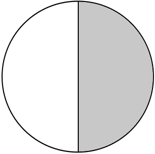
Figure 1: Half-balls are extremal sets for $K_{\rm mv}({\mathbb{B}}^{n})$

Symmetrization, and other ad hoc geometric arguments, enable us to restrict the analysis of possible extremal sets for $K_{\rm mv}({\mathbb{B}}^{n})$ to a two-parameter family of subsets of ${\mathbb{B}}^{n}$, which are the complement in ${\mathbb{B}}^{n}$ of another ball $B$.
Specifically, let $O$ and $P$ be the centers of ${\mathbb{B}}^{n}$ and $B$, and, with reference to Figure 2 (for $n=2$), let $E_{\vartheta,\varphi}={\mathbb{B}}^{n}\setminus B$, where $\vartheta$ denotes the angle between the positive $x_{1}$-half-axis and the radius of ${\mathbb{B}}^{n}$ issued from a point $M\in\partial{\mathbb{B}}^{n}\cap\partial B$, and $\varphi$ denotes the angle between the same half-axis and the radius of $B$ through $M$. The couple $(\vartheta,\varphi)$ belongs to the set

(3.3) $$\Upsilon=\{(\vartheta,\varphi):0<\vartheta<\pi,0\leq\varphi<\vartheta\}.$$

The endpoint case when $\varphi=0$ corresponds to the borderline situation when $B$ is a half-space, and hence $E_{\vartheta,0}$ is a spherical segment.
In fact, in the proof of Theorem 3.2, we shall only need to consider sets $E_{\vartheta,\varphi}$ such that $B\nsubseteq{\mathbb{B}}^{n}$, and

$${\cal H}^{n-1}(\partial^{M}E_{\vartheta,\varphi}\cap\partial{\mathbb{B}}^{n})\geq{\cal H}^{n-1}(\partial{\mathbb{B}}^{n}\setminus\partial^{M}E_{\vartheta,\varphi}),$$

namely couples $(\vartheta,\varphi)$ from the set

(3.4) $$\Theta=\{(\vartheta,\varphi)\in\mathbb{R}^{2}:\tfrac{\pi}{2}\leq\vartheta<\pi,\>0\leq\varphi<\vartheta\}.$$

Denote by $r$ the radius of $B$, and observe that, if $\varphi>0$, then

$$r=\frac{\sin\vartheta}{\sin\varphi}.$$

Relevant geometric quantities associated with the set $E_{\vartheta,\varphi}$ can be expressed in terms of the functions $\Psi_{k}$ and $\Phi_{k}$ defined, for $k\in\mathbb{N}\cup\{0\}$, by

(3.5) $$\Psi_{k}(t)=\int_{0}^{t}\sin^{k}\tau\,d\tau,$$

and

(3.6) $$\Phi_{k}(t)=\int_{0}^{t}\cos^{k}\tau\,d\tau,$$

for $t\in[0,\pi]$. The following equations are easily verified:

(3.7) $$\Psi_{k}(t)=\frac{k-1}{k}\Psi_{k-2}(t)-\frac{1}{k}\cos t\,\sin^{k-1}t,$$

(3.8) $$\Phi_{k}(t)=\frac{k-1}{k}\Phi_{k-2}(t)+\frac{1}{k}\cos^{k-1}t\sin t,$$

for $k\geq 2$ and $t\in[0,\pi]$.

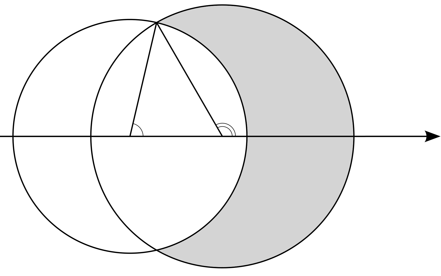
Figure 2: The set $E_{\vartheta,\varphi}$

Computations show that

(3.9) $${\cal H}^{n-1}(\partial^{M}E_{\vartheta,\varphi}\cap\partial{\mathbb{B}}^{n})=(n-1)\omega_{n-1}\Psi_{n-2}(\vartheta),$$

(3.10) $${\cal H}^{n-1}(\partial^{M}E_{\vartheta,\varphi}\cap{\mathbb{B}}^{n})=(n-1)\omega_{n-1}\Psi_{n-2}(\varphi)\Big{(}\frac{\sin\vartheta}{\sin\varphi}\Big{)}^{n-1},$$

for $(\vartheta,\varphi)\in\Upsilon$, where $\omega_{n}=|{\mathbb{B}}^{n}|$, namely $\omega_{n}=\frac{\pi^{n/2}}{\Gamma(1+n/2)}$. Moreover,

(3.11) $$|E_{\vartheta,\varphi}|=\omega_{n-1}\left(\Psi_{n}(\vartheta)-\Psi_{n}(\varphi)\left(\frac{\sin\vartheta}{\sin\varphi}\right)^{n}\right),$$

and

(3.12) $$|{\mathbb{B}}^{n}\setminus E_{\vartheta,\varphi}|=\omega_{n-1}\left(\Psi_{n}(\pi-\vartheta)+\Psi_{n}(\varphi)\left(\frac{\sin\vartheta}{\sin\varphi}\right)^{n}\right).$$

Note that equations (3.9)–(3.12) also hold for $\varphi=0$, which corresponds to the case when $E_{\vartheta,0}$ is the intersection of ${\mathbb{B}}^{n}$ with a half-space, provided that their right-hand sides are extended by continuity.
The following equations will be used below without further mentioning:

(3.13) $$\omega_{n}=\omega_{n-1}\Psi_{n}(\pi),$$

(3.14) $$n\omega_{n}=(n-1)\omega_{n-1}\Psi_{n-2}(\pi),$$

(3.15) $$\Psi_{k}(\pi)-\Psi_{k}(t)=\Psi_{k}(\pi-t),$$

(3.16) $$\Psi_{k}(t)-\Psi_{k}(\pi-\vartheta)=2\Phi_{k}(t-\tfrac{\pi}{2})$$

for $k\geq 0$ and $t\in[0,\pi]$.

Given a set $E\subset{\mathbb{B}}^{n}$, let us denote by ${\cal Q}_{\rm mv}(E)$ the quotient appearing in (2.6) for $\Omega={\mathbb{B}}^{n}$, namely

(3.17) $${\cal Q}_{\rm mv}(E)=\frac{|E|\,{\cal H}^{n-1}(\partial{\mathbb{B}}^{n}\setminus\partial^{M}E)+|{\mathbb{B}}^{n}\setminus E|\,{\cal H}^{n-1}(\partial^{M}E\cap\partial{\mathbb{B}}^{n})}{|{\mathbb{B}}^{n}|\,{\cal H}^{n-1}(\partial^{M}E\cap{\mathbb{B}}^{n})}.$$

In particular, owing to (3.9)–(3.11),

(3.18) $${\cal Q}_{\rm mv}(E_{\vartheta,\varphi})=\frac{\displaystyle n\omega_{n}^{2}-4(n-1)\omega_{n-1}^{2}\Phi_{n-2}(\vartheta-\tfrac{\pi}{2})\left(\Phi_{n}(\vartheta-\tfrac{\pi}{2})-\Psi_{n}(\varphi)\frac{\sin^{n}\vartheta}{\sin^{n}\varphi}\right)}{\displaystyle 2(n-1)\omega_{n-1}\omega_{n}\Psi_{n-2}(\varphi)\frac{\sin^{n-1}\vartheta}{\sin^{n-1}\varphi}}$$

for $(\vartheta,\varphi)\in\Theta$, where the expression on the right-hand side is extended by continuity for $\varphi=0$.

The following technical lemma will be needed in our proof of Theorem 3.2.

Lemma 3.3

Let $n\geq 2$, and let

$$\Lambda=\{(t,s)\in\mathbb{R}^{2}:0\leq t<\tfrac{\pi}{2},\>0\leq s<t+\tfrac{\pi}{2}\}.$$

Define the function $F:\Lambda\to\mathbb{R}$ as

(3.19) $$F(t,s)=\displaystyle 1-4\frac{n-1}{n}\frac{\omega_{n-1}^{2}}{\omega_{n}^{2}}\Phi_{n-2}(t)\left(\Phi_{n}(t)-\Psi_{n}(s)\frac{\cos^{n}t}{\sin^{n}s}\right)-(n-1)\Psi_{n-2}(s)\frac{\cos^{n-1}t}{\sin^{n-1}s}$$

for $(t,s)\in\Lambda$, where the right-hand side is extended by continuity for $s=0$. Then

(3.20) $$F(t,s)\leq F(0,0)=0\quad\hbox{for $(t,s)\in\Lambda$ ,}$$

and the equality holds in the first inequality only if $(t,s)=(0,0)$. Hence, $F$ attains its maximum in $\Lambda$ only at $(0,0)$.

Proof. Assume first that $t=0$. One has that

$$F(0,s)=1-(n-1)\frac{\Psi_{n-2}(s)}{\sin^{n-1}s},\qquad\hbox{for $s\in(0,\tfrac{\pi}{2}]$.}$$

If $g:[0,\tfrac{\pi}{2}]\to\mathbb{R}$ is the function defined by $g(s)=\sin^{n-1}s-(n-1)\Psi_{n-2}(s)$ for $s\in[0,\tfrac{\pi}{2}]$, then $g(0)=0$ and $g^{\prime}(s)<0$ for $s\in(0,\tfrac{\pi}{2}]$. Hence, inequality (3.20) follows for $t=0$.
Next, fix any $t\in(0,\tfrac{\pi}{2})$. Equation (3.7), with $k=n$, ensures that

(3.21) $$\frac{\partial F}{\partial s}(t,s)=(n-1)\frac{\cos^{n-1}t}{\sin^{n+1}t}\big{[}\sin^{n-1}s-(n-1)\Psi_{n-2}(s)\cos s\big{]}\big{[}C_{n}\Phi_{n-2}(t)\cos t-\sin s\big{]}$$

for $s\in(0,t+\tfrac{\pi}{2})$, where

(3.22) $$C_{n}=\frac{4\omega_{n-1}^{2}}{n\omega_{n}^{2}}.$$

It is easily seen that

$$\sin^{n-1}s-(n-1)\Psi_{n-2}(s)\cos s>0$$

for $s\in(0,\pi]$. Thus, on setting

(3.23) $$f_{n}(t)=C_{n}\Phi_{n-2}(t)\cos t,$$

one has that $\frac{\partial F}{\partial s}(t,s)=0$ if

(3.24) $$\sin s=f_{n}(t).$$

We claim that

(3.25) $$0<f_{n}(t)<1\qquad\hbox{for $t\in(0,\tfrac{\pi}{2})$.}$$

The first inequality in (3.25) is trivial. The second inequality can be established by induction. If $n=2$, then $f_{2}(t)=\frac{8}{\pi^{2}}t\cos t$, and an elementary analysis of $f_{2}^{\prime}(t)$ ensures that

$$\max_{t\in(0,\tfrac{\pi}{2}]}f_{2}(t)=\max_{t\in(0,\tfrac{\pi}{3}]}f_{2}(t)\leq\frac{8}{3\pi}<1.$$

If $n=3$, then $f_{3}(t)=\frac{3}{4}\sin t\cos t$, whence

$$f_{3}(t)\leq\frac{3}{4}<1\qquad\hbox{for $t\in(0,\tfrac{\pi}{2})$.}$$

Finally,

$$f_{n+2}(t)=C_{n+2}\Phi_{n}(t)\cos t\leq C_{n+2}\Phi_{n-2}(t)\cos t=\frac{n(n+2)}{(n+1)^{2}}f_{n}(t)\leq f_{n}(t),$$

for every $n\geq 2$, where the first inequality holds since $\Phi_{n}\leq\Phi_{n-2}$. This completes the proof of (3.25).
As a consequence of (3.25), equation (3.24) admits an unique solution $s_{t}$ in $(0,\tfrac{\pi}{2}]$, given by

(3.26) $$s_{t}=\arcsin(C_{n}\Phi_{n-2}(t)\cos t).$$

Moreover, $C_{n}\Phi_{n-2}(t)\cos t-\sin s<0$, if $s_{t}<s<\min\{\pi-s_{t},t+\tfrac{\pi}{2}\}$, and $C_{n}\Phi_{n-2}(t)\cos t-\sin s\geq 0$ otherwise. Hence,

(3.27) $$\sup_{s\in(0,t+\tfrac{\pi}{2})}F(t,s)=\max\Big{\{}F(t,s_{t}),\lim_{s\rightarrow(t+\tfrac{\pi}{2})^{-}}F(t,s)\Big{\}}.$$

Thus, inequality (3.20) will follow if we show that

(3.28) $$\lim_{s\rightarrow(t+\tfrac{\pi}{2})^{-}}F(t,s)<0$$

and $F(t,s_{t})<0$, namely

(3.29) $$\Phi_{n}(t)\sin s_{t}+\frac{\cos^{n}t}{\sin^{n-1}s_{t}}(\Psi_{n-2}(s_{t})-\Psi_{n}(s_{t}))-\frac{1}{n-1}\cos t>0.$$

As far as inequality (3.28) is concerned, note that

(3.30) $$\lim_{s\rightarrow(t+\tfrac{\pi}{2})^{-}}F(t,s) =\displaystyle 1-4\frac{n-1}{n}\frac{\omega_{n-1}^{2}}{\omega_{n}^{2}}\textstyle\Phi_{n-2}(t)\left(\Phi_{n}(t)-\Psi_{n}(t+\tfrac{\pi}{2})\right)-(n-1)\Psi_{n-2}(t+\tfrac{\pi}{2})=$$

$$=\Big{(}1+\frac{2(n-1)\omega_{n-1}}{n\omega_{n}}\Phi_{n-2}(t)\Big{)}\left(1-\frac{n\omega_{n}}{2\omega_{n-1}}\right),$$

where the second equality holds thanks to the fact that

$$\Psi_{n}(t+\tfrac{\pi}{2})=\Psi_{n}(\tfrac{\pi}{2})+\Phi_{n}(t)=\frac{\omega_{n}}{2\omega_{n-1}}+\Phi_{n}(t),$$

and

$$\Psi_{n-2}(t+\tfrac{\pi}{2})=\Psi_{n-2}(\tfrac{\pi}{2})+\Phi_{n-2}(t)=\frac{n\omega_{n}}{2(n-1)\omega_{n-1}}+\Phi_{n-2}(t).$$

Observe that

(3.31) $$a_{n}=\frac{n\omega_{n}}{\omega_{n-1}}>2\qquad\hbox{for $n\geq 2$.}$$

Inequality (3.31) follows by induction, from the fact that $a_{2}=\pi>2$, $a_{3}=4>1$ and

(3.32) $$a_{n+2}=\frac{n+1}{n}a_{n}>a_{n},$$

for $n\geq 2$, inasmuch as

(3.33) $$\frac{a_{n+2}}{a_{n}}=\frac{\frac{(n+2)\omega_{n+2}}{\omega_{n+1}}}{\frac{n\omega_{n}}{\omega_{n-1}}}=\frac{n+2}{n}\frac{\Gamma(1+\frac{n}{2})\Gamma(1+\frac{n+1}{2})}{\Gamma(1+\frac{n+2}{2})\Gamma(1+\frac{n-1}{2})}=\frac{n+2}{n}\frac{n+1}{n+2}=\frac{n+1}{n}.$$

Equation (3.28) is a consequence of (3.30) and (3.31).
Let us now focus on inequality (3.29). We begin by showing that

(3.34) $$\Psi_{n-2}(s)-\Psi_{n}(s)\geq\frac{1}{n-1}\sin^{n-1}s-\frac{1}{n+2}\sin^{n+1}s\qquad\hbox{for $s\in[0,\tfrac{\pi}{2}]$.}$$

To see this, define $h:[0,\tfrac{\pi}{2}]\to\mathbb{R}$ as

$$h(s)=\Psi_{n-2}(s)-\Psi_{n}(s)-\frac{1}{n-1}\sin^{n-1}s+\frac{1}{n+2}\sin^{n+1}s\quad\hbox{for $s\in[0,\tfrac{\pi}{2}]$,}$$

and notice that

$$h^{\prime}(s)=h_{1}(s)\sin^{n-2}s\cos s\quad\hbox{for $s\in[0,\tfrac{\pi}{2}]$,}$$

where $h_{1}(s)=\cos s-1+\frac{n+1}{n+2}\sin^{2}s$. An analysis of the monotonicity properties of $h_{1}$ tells us that there exists $\bar{s}\in(0,\tfrac{\pi}{2})$ such that $h(s)$ is increasing in $[0,\bar{s}]$ and decreasing in $[\bar{s},\tfrac{\pi}{2}]$. Therefore, inequality (3.34) will follow if we show that

(3.35) $$\Psi_{n-2}(\tfrac{\pi}{2})-\Psi_{n}(\tfrac{\pi}{2})-\frac{1}{n-1}+\frac{1}{n+2}>0.$$

Since

$$\Psi_{n}(\tfrac{\pi}{2})=\frac{\omega_{n}}{2\omega_{n-1}}\quad\hbox{and}\quad\Psi_{n-2}(\tfrac{\pi}{2})=\frac{n\omega_{n}}{2(n-1)\omega_{n-1}},$$

on setting

$$b_{n}=\frac{(n+2)\omega_{n}}{\omega_{n-1}},$$

inequality (3.35) is equivalent to

(3.36) $$b_{n}>6\qquad\hbox{for $n\geq 2$.}$$

Inequality (3.36) trivially holds for $n=2,3$. Also,

$$b_{n+2}=(n+4)\frac{\omega_{n+2}}{\omega_{n+1}}=b_{n}\frac{(n+4)(n+1)}{(n+2)^{2}}>b_{n}$$

for $n\geq 2$. Hence, inequality (3.36) follows by induction. The proof of (3.34) is thereby complete.
On recalling (3.26) and (3.34), and making use of (3.8), in order to accomplish the prove of inequality (3.29) it thus suffices to show that

(3.37) $$\frac{n-1}{n}C_{n}\Phi_{n-2}(t)^{2}-\frac{1-\cos^{n-1}t}{n-1}+C_{n}\Phi_{n-2}(t)\cos^{n-1}t\left(\frac{\sin t}{n}-\frac{C_{n}}{n+2}\Phi_{n-2}(t)\cos^{2}t\right)>0.$$

Assume first that $n\geq 3$, and define the functions

(3.38) $$k_{n}(t)=\frac{n-1}{n}C_{n}\Phi_{n-2}(t)^{2}-\frac{1-\cos^{n-1}t}{n-1},$$

(3.39) $$\kappa_{n}(t)=\frac{\sin t}{n}-\frac{C_{n}}{n+2}\Phi_{n-2}(t)\cos^{2}t$$

for $t\in(0,\tfrac{\pi}{2})$. Let us first take into account the function $k_{n}$. If $n=3$, then

(3.40) $$k_{3}(t)=0\qquad\hbox{ for every $t\in(0,\tfrac{\pi}{2})$.}$$

When $n\geq 4$, one has that

$$k_{n}^{\prime}(t)=\left(2\frac{n-1}{n}C_{n}\Phi_{n-2}(t)-\sin t\right)\cos^{n-2}t.$$

We claim that there exists $\bar{t}\in(0,\tfrac{\pi}{2})$ such that $k_{n}(t)$ is increasing in $(0,\bar{t}\,]$ and decreasing in $[\bar{t},\tfrac{\pi}{2})$. Our claim follows from the fact that $k_{n}^{\prime}(0)=0$ and

(3.41) $$2\frac{n-1}{n}C_{n}\Phi_{n-2}(\tfrac{\pi}{2})<1.$$

The latter property is in turn a consequence of the equality

$$2\frac{n-1}{n}C_{n}\Phi_{n-2}(\tfrac{\pi}{2})=\frac{4\omega_{n-1}}{n\omega_{n}}=\frac{4}{a_{n}},$$

where $a_{n}$ is the sequence defined by (3.31), owing to (3.32), and to the fact that $a_{3}=4$ and that $a_{4}=\frac{8}{3}\pi>4$, by the first equality in (3.33). Altogether, since $k_{n}(0)=k_{n}(\tfrac{\pi}{2})=0$, we have proved that, if $n\geq 4$, then

(3.42) $$k_{n}(t)>0\qquad\hbox{for $t\in(0,\tfrac{\pi}{2})$.}$$

Consider next the function $\kappa_{n}$. One has that

(3.43) $$\kappa_{n}^{\prime}(t)=\frac{\cos t}{n}\left(1-\frac{nC_{n}}{n+2}\cos^{n-1}t+\frac{2nC_{n}}{n+2}\Phi_{n-2}(t)\sin t\right)\quad\hbox{for $t\in(0,\tfrac{\pi}{2})$.}$$

We claim that

(3.44) $$\frac{n}{n+2}C_{n}<1\quad\hbox{for $n\geq 2$.}$$

To verify inequality (3.44), observe that both the subsequence $\frac{2n}{2n+2}C_{2n}$ and the subsequence $\frac{2n+1}{(2n+1)+2}C_{2n+1}$ are increasing. This is a consequence of the inequality $\frac{n}{n+2}C_{n}<\frac{n+2}{n+4}C_{n+2}$, which holds for every $n\geq 2$ and follows from the fact that $\Gamma(s+1)=s\Gamma(s)$ for every $s\in\mathbb{R}$. On the other hand, Stirling’s formula implies that

$$\frac{n}{n+2}C_{n}=\frac{4\omega_{n-1}^{2}}{(n+2)\omega_{n}^{2}}\leq\lim_{n}\frac{4\omega_{n-1}^{2}}{(n+2)\omega_{n}^{2}}=\tfrac{\pi}{2}<1.$$

Combining these pieces of information yields inequality (3.44). Owing to this inequality, we infer from (3.43) that $\kappa_{n}^{\prime}(t)>0$ for $t\in(0,\tfrac{\pi}{2})$. Hence, since $\kappa_{n}(0)=0$,

(3.45) $$\kappa_{n}(t)>0\qquad\hbox{for $t\in(0,\tfrac{\pi}{2})$.}$$

Coupling either (3.40) or (3.42), with (3.45) yields (3.37), and hence inequality (3.29) for $n\geq 3$.

Let us finally consider the case when $n=2$. Observe that, in this case, the left-hand side of (3.37) equals

$$\tilde{k}+C_{2}\Phi_{0}(t)\tilde{\kappa}(t)\cos t\qquad\hbox{for $t\in(0,\tfrac{\pi}{2})$,}$$

where we have set

(3.46) $$\tilde{k}(t)=k_{2}(t)+\frac{16}{\pi^{4}}t^{2}\cos t=\frac{4}{\pi^{4}}t^{2}(\pi^{2}+4\cos t)-1+\cos t,$$

(3.47) $$\tilde{\kappa}(t)=\kappa_{2}(t)-\frac{2}{\pi^{2}}t=\frac{1}{2}\sin t-\frac{2}{\pi^{2}}t(1+\cos^{2}t).$$

We claim that

(3.48) $$m_{1}(t)\equiv t-\frac{\pi^{2}}{2}\sqrt{\frac{1-\cos t}{\pi^{2}+4\cos t}}>0 \hbox{for $t\in(0,\tfrac{\pi}{2})$},$$

(3.49) $$m_{2}(t)\equiv\frac{\sin t}{1+\cos^{2}t}-\frac{4}{\pi^{2}}t>0 \qquad\hbox{for $t\in(0,\tfrac{\pi}{2})$}.$$

Inequalities (3.48) and (3.49) imply $\tilde{k}(t)>0$ and $\tilde{\kappa}(t)>0$, and hence (3.37) follows, thus establishing inequality (3.29) also for $n=2$. It just remains to prove inequalities (3.48) and (3.49). An analysis of monotonicity properties of the function $m_{1}(t)$ tells us that there exists $\tilde{t}\in(0,\tfrac{\pi}{2})$ such that $m_{1}(t)$ is increasing in $(0,\tilde{t}\,]$ and decreasing in $[\tilde{t},\tfrac{\pi}{2})$. Inequality (3.48) hence follows, since $m_{1}(0^{+})=m_{1}(\tfrac{\pi}{2}^{-})=0$.
As for (3.49), a study of the sign of $m_{2}^{\prime\prime}(t)$ tells us that there exists $\hat{t}\in(0,\tfrac{\pi}{2})$ such that $m_{2}(t)$ is convex in $(0,\hat{t}\,]$, and concave in $[\hat{t},\tfrac{\pi}{2})$. This piece of information, combined with the fact that $m_{2}(0^{+})=0$, $m_{2}^{\prime}(0^{+})=\frac{\pi^{2}-8}{2\pi^{2}}>0$ and $m_{2}(\tfrac{\pi}{2}^{-})=\frac{\pi-2}{\pi}>0$, yields (3.49).        

Given a measurable set $E\subset{\mathbb{B}}^{n}$, we denote by $E^{\sharp}$ the spherical symmetral of $E$ about the half-axis $X=\{(x_{1},\dots,x_{n}):x_{1}\geq 0,x_{2}=\dots=x_{n}=0\}$. The set $E^{\sharp}$ is defined as the subset of ${\mathbb{B}}^{n}$ such that the intersection of $E^{\sharp}$ with any sphere $S$ centered at $0$ is a spherical cap, centered at $S\cap X$, such that ${\cal H}^{n-1}(E^{\sharp}\cap S)={\cal H}^{n-1}(E\cap S)$. In particular, $E^{\sharp}$ is symmetric about the $x_{1}$-axis.
The very definition of spherical symmetrization, and the use of polar coordinates, ensure that

(3.50) $$|E|=|E^{\sharp}|$$

for every measurable subset $E$ of ${\mathbb{B}}^{n}$. The definition of spherical symmetrization again tells us that

(3.51) $${\cal H}^{n-1}(\partial E^{\sharp}\cap\partial{\mathbb{B}}^{n})={\cal H}^{n-1}(\partial E\cap\partial{\mathbb{B}}^{n})$$

if $E$ is a sufficiently regular subset of ${\mathbb{B}}^{n}$. Moreover, a classical property of spherical symmetrization entails that it does not increase perimeter relative to ${\mathbb{B}}^{n}$ of regular subsets $E$ of ${\mathbb{B}}^{n}$; namely

(3.52) $${\cal H}^{n-1}(\partial E^{\sharp}\cap{\mathbb{B}}^{n})\leq{\cal H}^{n-1}(\partial E\cap{\mathbb{B}}^{n}),$$

see e.g. [Ka]. In fact, equations (3.51) and (3.52) will be exploited when $E$ is just the intersection of ${\mathbb{B}}^{n}$ with a polyhedron. This will suffice for our purposes, since we shall make use of a result from [Ma3, Lemma 9.4.1/3] which tells us that, given any measurable set $E\subset{\mathbb{B}}^{n}$ such that ${\cal H}^{n-1}(\partial^{M}E)<\infty$, there exists a sequence of polyhedra $\{P_{k}\}$ in ${{\mathbb{R}}^{n}}$ with the following properties. Define $Q_{k}=P_{k}\cap{\mathbb{B}}^{n}$ for $k\in\mathbb{N}$. Then

(3.53) $$\lim_{k\to\infty}\chi_{Q_{k}}=\chi_{E}$$

in $L^{1}({\mathbb{B}}^{n})$,

(3.54) $$\lim_{k\to\infty}{\cal H}^{n-1}(\partial Q_{k}\cap{\mathbb{B}}^{n})={\cal H}^{n-1}(\partial^{M}E\cap{\mathbb{B}}^{n}),$$

and

(3.55) $$\lim_{k\to\infty}{\cal H}^{n-1}(\partial Q_{k}\cap\partial{\mathbb{B}}^{n})={\cal H}^{n-1}(\partial^{M}E\cap\partial{\mathbb{B}}^{n}).$$

Proof of Theorem 3.2. Let ${\cal Q}_{\rm mv}$ be the functional defined by (3.17). Since for any measurable set $E\subset{\mathbb{B}}^{n}$ such that ${\cal H}^{n-1}(\partial^{M}E)<\infty$ there exists a sequence of polyhedra $\{P_{k}\}$ satisfying (3.53)–(3.55), one has that

(3.60) $$\sup_{E\subset{\mathbb{B}}^{n}}{\cal Q}_{\rm mv}(E) =\sup_{\tiny\begin{array}[]{c}{Q=P\cap{\mathbb{B}}^{n}}\\ P\hbox{ is a polyhedron}\end{array}}{\cal Q}_{\rm mv}(Q)\leq\sup_{\tiny\begin{array}[]{c}{Q=P\cap{\mathbb{B}}^{n}}\\ P\hbox{ is a polyhedron}\end{array}}{\cal Q}_{\rm mv}(Q^{\sharp})$$

(3.63) $$\leq\sup_{\tiny\begin{array}[]{c}{E\subset{\mathbb{B}}^{n}}\\ E=E^{\sharp}\end{array}}{\cal Q}_{\rm mv}(E)\leq\sup_{E\subset{\mathbb{B}}^{n}}{\cal Q}_{\rm mv}(E).$$

Note that the first equality in (3.60) holds by (3.53)–(3.55), and the first inequality by (3.50) and (3.51). Hence,

$$K_{\rm mv}({\mathbb{B}}^{n})=\sup_{E\subset{\mathbb{B}}^{n}}{\cal Q}_{\rm mv}(E)=\sup_{\tiny\begin{array}[]{c}{E\subset{\mathbb{B}}^{n}}\\ E=E^{\sharp}\end{array}}{\cal Q}_{\rm mv}(E).$$

Thus, we may limit ourselves to maximize ${\cal Q}_{\rm mv}(E)$ in the class of sets $E$ such that $E=E^{\sharp}$, and hence, in particular, $\partial^{M}E\cap\partial{\mathbb{B}}^{n}$ is a spherical cap (or an empty set) on $\partial{\mathbb{B}}^{n}$. Since the functional ${\cal Q}_{\rm mv}(E)$ is invariant under replacements of $E$ with ${\mathbb{B}}^{n}\setminus E$, we may also assume that ${\cal H}^{n-1}(\partial^{M}E\cap\partial{\mathbb{B}}^{n})\geq{\cal H}^{n-1}(\partial{\mathbb{B}}^{n}\setminus\partial^{M}E)$. Let us also observe that ${\cal Q}_{\rm mv}(E)$ cannot achieve its maximum at any set $E$ such that ${\cal H}^{n-1}(\partial{\mathbb{B}}^{n}\setminus\partial^{M}E)=0$. Indeed, if this equality holds, then ${\cal H}^{n-1}(\partial^{M}E\cap{\mathbb{B}}^{n})={\cal H}^{n-1}(\partial^{M}({\mathbb{B}}^{n}\setminus E)\cap{\mathbb{B}}^{n})={\cal H}^{n-1}(\partial^{M}({\mathbb{B}}^{n}\setminus E))$, and hence

(3.64) $${\cal Q}_{\rm mv}(E)=\frac{|{\mathbb{B}}^{n}\setminus E|{\cal H}^{n-1}(\partial{\mathbb{B}}^{n})}{|{\mathbb{B}}^{n}|{\cal H}^{n-1}(\partial^{M}({\mathbb{B}}^{n}\setminus E))}\leq 1<\frac{n\omega_{n}}{2\omega_{n-1}}.$$

Observe that the last inequality in (3.64) holds by (3.31). The first inequality is instead a consequence of the fact that, by the standard isoperimetric theorem, the ratio $\frac{|{\mathbb{B}}^{n}\setminus E|}{{\cal H}^{n-1}(\partial^{M}({\mathbb{B}}^{n}\setminus E))}$ does not decrease if ${\mathbb{B}}^{n}\setminus E$ is replaced with a ball of equal Lebesgue measure, and that it increases if the ball is replaced with a larger ball. On the other hand, the rightmost side of (3.64) agrees with the functional ${\cal Q}_{\rm mv}$ evaluated at a half-ball. Altogether,

(3.65) $$\sup_{E\subset{\mathbb{B}}^{n}}{\cal Q}_{\rm mv}(E)=\sup_{E\in\mathcal{E}}{\cal Q}_{\rm mv}(E)\,,$$

where

(3.66) $$\mathcal{E}=\{E\subset{\mathbb{B}}^{n}:E\,\hbox{is measurable}\,,E=E^{\sharp},\,{\cal H}^{n-1}(\partial^{M}E\cap\partial{\mathbb{B}}^{n})\geq{\cal H}^{n-1}(\partial{\mathbb{B}}^{n}\setminus\partial^{M}E)>0\}.$$

Given $t\in\mathbb{R}$, define the half-space

(3.67) $$H_{t}=\{x\in\mathbb{R}^{n}:x_{1}>t\},$$

and set $\bar{t}=\sup\{t\in\mathbb{R}:H_{t}\supset\partial^{M}E\cap\partial{\mathbb{B}}^{n}\}$. Then either $|H_{\bar{t}}\cap{\mathbb{B}}^{n}|>|E|$, or $|H_{\bar{t}}\cap{\mathbb{B}}^{n}|\leq|E|$.
Assume first that $|H_{\bar{t}}\cap{\mathbb{B}}^{n}|>|E|$, and consider a ball $B$ such that $B\cap\partial{\mathbb{B}}^{n}=\partial H_{\bar{t}}\cap\partial{\mathbb{B}}^{n}$ and $|{\mathbb{B}}^{n}\setminus B|=|E|$. Define

$$\widetilde{E}=({\mathbb{B}}^{n}\backslash E)\cup(B\backslash{\mathbb{B}}^{n}).$$

Clearly,

$$|\widetilde{E}|=|B|,$$

and, by the isoperimetric property of the ball,

$${\cal H}^{n-1}(\partial\widetilde{E})\geq{\cal H}^{n-1}(\partial B).$$

On the other hand,

$${\cal H}^{n-1}(\partial\widetilde{E})={\cal H}^{n-1}(\partial B\cap({{\mathbb{R}}^{n}}\setminus{\mathbb{B}}^{n}))+{\cal H}^{n-1}(\partial^{M}E\cap{\mathbb{B}}^{n}),$$

and

$${\cal H}^{n-1}(\partial B)={\cal H}^{n-1}(\partial B\cap({{\mathbb{R}}^{n}}\setminus{\mathbb{B}}^{n}))+{\cal H}^{n-1}(\partial B\cap{\mathbb{B}}^{n}).$$

Hence,

$${\cal H}^{n-1}(\partial B\cap{\mathbb{B}}^{n})\leq{\cal H}^{n-1}(\partial^{M}E\cap{\mathbb{B}}^{n}).$$

On setting $\widehat{E}={\mathbb{B}}^{n}\backslash B$, one has that $|\widehat{E}|=|E|$ and

$${\cal Q}_{\rm mv}(E)\leq{\cal Q}_{\rm mv}(\widehat{E}).$$

Suppose next that $|H_{\bar{t}}\cap{\mathbb{B}}^{n}|\leq|E|$. Then the set $\widehat{E}=H_{\bar{t}}\cap{\mathbb{B}}^{n}$ satisfies the inequalities $|\widehat{E}|\leq|E|$, and ${\cal H}^{n-1}(\partial E\cap{\mathbb{B}}^{n})\geq{\cal H}^{n-1}(\partial H_{\bar{t}}\cap{\mathbb{B}}^{n})={\cal H}^{n-1}(\partial\widehat{E}\cap{\mathbb{B}}^{n})$, whence

$${\cal Q}_{\rm mv}(E)\leq{\cal Q}_{\rm mv}(\widehat{E}).$$

Altogether, we have shown that

(3.68) $$K_{\rm mv}({\mathbb{B}}^{n})=\sup_{\scriptstyle E\in{\cal A}}{\cal Q}_{\rm mv}(E),$$

where ${\cal A}$ denotes the collection of those subsets $E$ of ${\mathbb{B}}^{n}$ such that $E$ is the complement in ${\mathbb{B}}^{n}$ of either a ball, or of a half-space, with ${\cal H}^{n-1}(\partial^{M}E\cap\partial{\mathbb{B}}^{n})\geq{\cal H}^{n-1}(\partial{\mathbb{B}}^{n}\setminus\partial^{M}E)>0$.
In view of (3.68), in order to conclude our proof it remains to show that

(3.69) $$\sup_{\scriptstyle E\in{\cal A}}{\cal Q}_{\rm mv}(E)\leq\frac{n\omega_{n}}{2\omega_{n-1}}.$$

We may thus focus on the case when $E=E_{\vartheta,\varphi}$ for some $(\vartheta,\varphi)\in\Theta$, where $\Theta$ is defined in (3.4). In other words, we have to show that

(3.70) $${\cal Q}_{\rm mv}(E_{\vartheta,\varphi})\leq\frac{n\omega_{n}}{2\omega_{n-1}},\qquad(\vartheta,\varphi)\in\Theta,$$

the equality being attained if $(\vartheta,\varphi)=(\tfrac{\pi}{2},0)$, in which case $E_{\tfrac{\pi}{2},0}$ is a half-ball.
Owing to formula (3.18), the conclusion follows from Lemma 3.3.        

4 A trace inequality on $\mathbb{B}^{n}$ with median normalization

Our concern in this section is to detect the extremal functions in the Poincaré trace inequality

(4.1) $$\|\widetilde{u}-{\rm med}_{{\mathbb{B}}^{n},\sigma}(u)\|_{L^{1}(\partial{\mathbb{B}}^{n})}\leq C_{\rm med}({\mathbb{B}}^{n},\sigma)\|Du\|({\mathbb{B}}^{n}),$$

with optimal constant $C_{\rm med}({\mathbb{B}}^{n},\sigma)$, for $u\in BV({\mathbb{B}}^{n})$. Recall that ${\rm med}_{{\mathbb{B}}^{n},\sigma}(u)$ denotes the $\sigma$-median of $u$, defined as in (2.27), which agrees with the usual median ${\rm med}_{{\mathbb{B}}^{n}}(u)$ when $\sigma=\tfrac{1}{2}$.
This is the content of the following theorem.

Theorem 4.1

Let $n\geq 2$ and let $\sigma\in(0,1)$. Set $\rho=\max\{\sigma,1-\sigma\}$. Then equality holds in (4.1) if $u$ is the characteristic function of the half-moon shaped set $E_{\vartheta_{\rho},\varphi_{\rho}}$ as in Figure 2, where $(\vartheta_{\rho},\varphi_{\rho})$ is the unique solution in the set $\Upsilon$ (defined by (3.3)) to the system

(4.2) $$\quad\left\{\begin{array}[]{l}\displaystyle\frac{\Psi_{n-2}(\varphi)}{\Psi_{n-2}(\vartheta)}\frac{\sin^{n}\vartheta}{\sin^{n}\varphi}=1-{\frac{\rho(n-1)\Psi_{n-2}(\pi)\cos\vartheta}{(n-1)\cos\vartheta\,\Psi_{n-2}({\vartheta})-\sin^{n-1}\vartheta}}\\ \\ \displaystyle\frac{\cos\varphi}{\sin\varphi}=\frac{\cos\vartheta}{\sin\vartheta}\left(1-{\frac{\rho(n-1)\Psi_{n-2}(\pi)}{(n-1)\cos^{2}\vartheta\,\Psi_{n-2}({\vartheta})-\sin^{n-1}\vartheta\cos\vartheta}}\right).\end{array}\right.$$

Theorem 4.1 follows from Theorem 2.4, via the next result.

Theorem 4.2

Let $n\geq 2$ and let $\sigma\in(0,1)$. Then the set $E_{\vartheta_{\sigma},\varphi_{\sigma}}$, defined as in Theorem 4.1 with $\rho$ replaced with $\sigma$, is extremal for $K_{\rm med}({\mathbb{B}}^{n},\sigma)$ (Figure 3).

Theorem 4.2 is in turn a straightforward consequence of Lemmas 4.3 and 4.4 below. The former enables us to reduce the detection of extremals for $K_{\rm med}({\mathbb{B}}^{n},\sigma)$ to the class of sets of the form $E_{\vartheta,\varphi}$ with $(\vartheta_{\rho},\varphi_{\rho})\in\Upsilon$. The latter identifies $E_{\vartheta_{\sigma},\varphi_{\sigma}}$, with $(\vartheta_{\sigma},\varphi_{\sigma})$ solving (4.2) with $\rho$ replaced with $\sigma$, as the unique extremal for $K_{\rm med}({\mathbb{B}}^{n},\sigma)$ in this special class.

In what follows, we denote by ${\cal Q}_{\rm med}(E)$ the functional of $E$ that is maximized on the right-hand side of (2.29), namely

(4.3) $${\cal Q}_{\rm med}(E)=\frac{{\cal H}^{n-1}(\partial^{M}E\cap\partial{\mathbb{B}}^{n})}{{\cal H}^{n-1}(\partial^{M}E\cap{\mathbb{B}}^{n})}.$$

We also set

(4.4) $${\cal B}=\{E\subset{\mathbb{B}}^{n}:E={\mathbb{B}}^{n}\setminus B,\hbox{$B$ is a ball or a half-space}\,{\cal H}^{n-1}(\partial{\mathbb{B}}^{n}\setminus\partial^{M}E)>0\}.$$

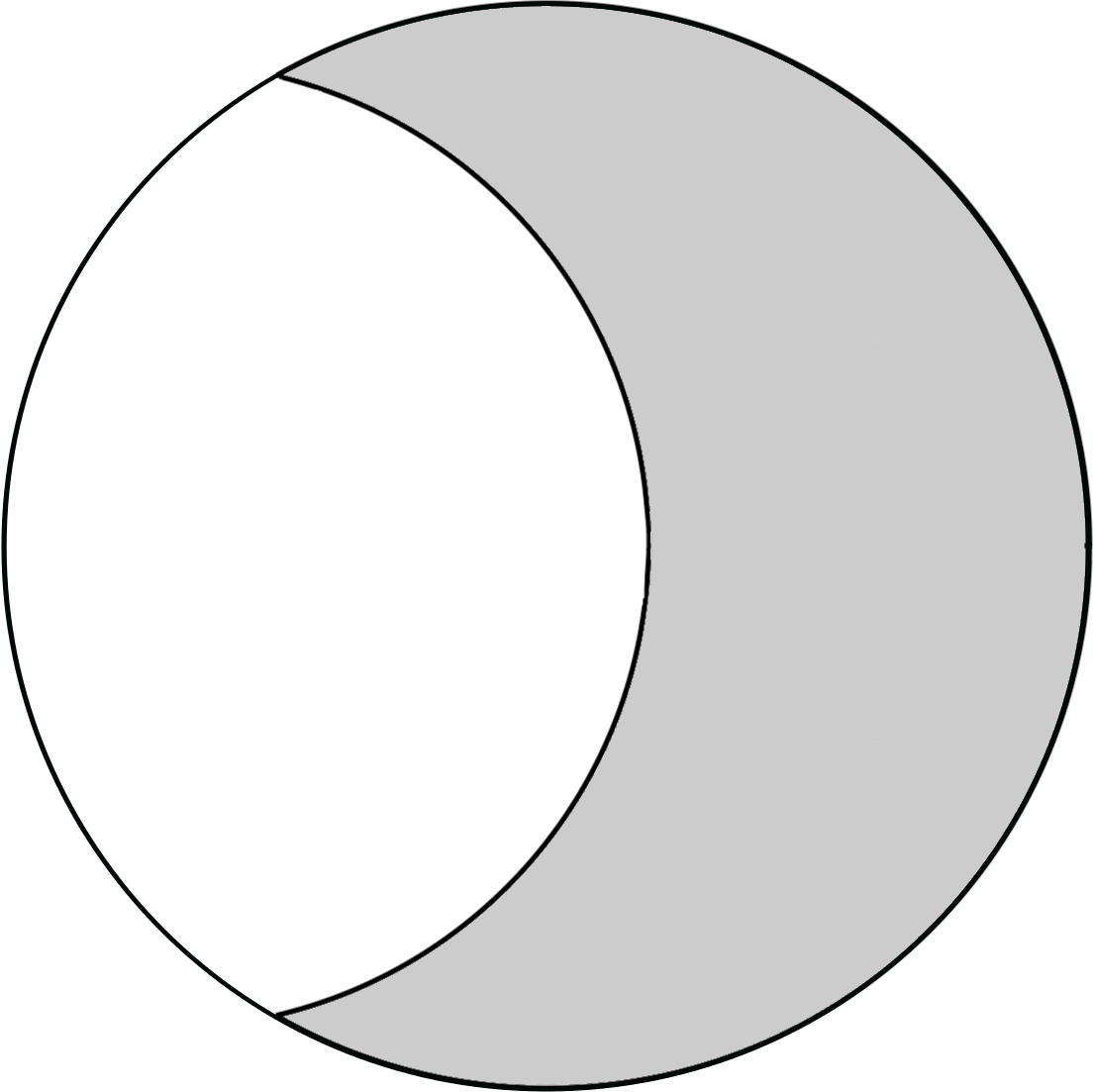
Figure 3: A half-moon shaped extremal set for $K_{\rm med}({\mathbb{B}}^{n},\sigma)$

Lemma 4.3

Let $n\geq 2$, and let $\sigma\in(0,1)$. Then,

(4.5) $$\sup_{|E|\leq\sigma|{\mathbb{B}}^{n}|}{\cal Q}_{\rm med}(E)=\sup_{\tiny\begin{array}[]{c}{E\in\cal{B}}\\ |E|=\sigma|{\mathbb{B}}^{n}|\end{array}}{\cal Q}_{\rm med}(E),$$

where ${\cal B}$ is defined by (4.4).

Proof. Given any measurable set $E\subset{\mathbb{B}}^{n}$ of finite perimeter in ${\mathbb{B}}^{n}$, consider a sequence of polyhedra $\{P_{k}\}$ satisfying (3.53)–(3.55). Fix any $k\in\mathbb{N}$. By properties (3.51) and (3.52) of spherical symmetrization, for every $\varepsilon>0$ and $\delta\in(0,1-\sigma)$, there exists $\overline{k}\in\mathbb{N}$ such that, if $k\geq\overline{k}$, then

(4.6) $$|Q_{k}^{\sharp}|\leq(1+\delta)|E|\,,$$

and

(4.7) $${\cal Q}_{\rm med}(E)\leq\frac{{\cal H}^{n-1}(\partial Q_{k}^{\sharp}\cap\partial{\mathbb{B}}^{n})+\varepsilon}{{\cal H}^{n-1}(\partial Q_{k}^{\sharp}\cap{\mathbb{B}}^{n})-\varepsilon}.$$

Owing to the arbitrariness of $\varepsilon$, inequalities (4.6) and (4.7) imply that

(4.8) $$\sup_{|E|\leq\sigma|{\mathbb{B}}^{n}|}{\cal Q}_{\rm med}(E)\leq\sup_{\tiny\begin{array}[]{c}{E=E^{\sharp}}\\ |E|\leq(\sigma+\delta)|{\mathbb{B}}^{n}|\end{array}}{\cal Q}_{\rm med}(E).$$

We next show that, for every $\delta$ as above,

(4.9) $$\sup_{\tiny\begin{array}[]{c}{E=E^{\sharp}}\\ |E|\leq(\sigma+\delta)|{\mathbb{B}}^{n}|\end{array}}{\cal Q}_{\rm med}(E)=\sup_{\tiny\begin{array}[]{c}{E\in\cal B}\\ |E|\leq(\sigma+\delta)|{\mathbb{B}}^{n}|\end{array}}{\cal Q}_{\rm med}(E).$$

An argument analogous to that in the proof of (3.64) tells us that, if $E$ is any subset of ${\mathbb{B}}^{n}$ such that ${\cal H}^{n-1}(\partial{\mathbb{B}}^{n}\setminus\partial^{M}E)=0$, then

$${\cal Q}_{\rm med}(E)=\frac{{\cal H}^{n-1}(\partial{\mathbb{B}}^{n})}{{\cal H}^{n-1}(\partial({\mathbb{B}}^{n}\setminus E))}\leq 1<\frac{n\omega_{n}}{2\omega_{n-1}}.$$

Moreover, the last expression agree with the functional ${\cal Q}_{\rm med}$ evaluated at a half-ball in ${\mathbb{B}}^{n}$. We may thus assume that the sets $E$ on the right-hand side of (4.9) fulfil the condition

(4.10) $${\cal H}^{n-1}(\partial{\mathbb{B}}^{n}\setminus\partial^{M}E)>0.$$

Let $E$ be subset of ${\mathbb{B}}^{n}$ such that $E=E^{\sharp}$, $|E|\leq(\sigma+\delta)|{\mathbb{B}}^{n}|$ and (4.10) holds. Define $\bar{t}=\sup\{t\in\mathbb{R}:H_{t}\supset\partial^{M}E\cap\partial{\mathbb{B}}^{n}\}$, where $H_{t}$ stands for the half-space introduced in the proof of Theorem 3.2. Assume first that $|H_{\bar{t}}\cap{\mathbb{B}}^{n}|>|E|$. Consider a ball $\widehat{B}$ such that $\widehat{B}\cap\partial{\mathbb{B}}^{n}=\partial H_{\bar{t}}\cap\partial{\mathbb{B}}^{n}$ and $|{\mathbb{B}}^{n}\backslash\widehat{B}|=|E|$. Set

$$\widetilde{E}=({\mathbb{B}}^{n}\backslash E)\cup(\widehat{B}\backslash{\mathbb{B}}^{n}).$$

Clearly,

$$|\widetilde{E}|=|\widehat{B}|,$$

and, by the isoperimetric property of the ball,

$${\cal H}^{n-1}(\partial\widetilde{E})\geq{\cal H}^{n-1}(\partial\widehat{B}).$$

On the other hand,

$${\cal H}^{n-1}(\partial\widetilde{E})={\cal H}^{n-1}(\partial\widehat{B}\cap({{\mathbb{R}}^{n}}\setminus{\mathbb{B}}^{n}))+{\cal H}^{n-1}(\partial^{M}E\cap{\mathbb{B}}^{n}),$$

and

$${\cal H}^{n-1}(\partial\widehat{B})={\cal H}^{n-1}(\partial\widehat{B}\cap({{\mathbb{R}}^{n}}\setminus{\mathbb{B}}^{n}))+{\cal H}^{n-1}(\partial\widehat{B}\cap{\mathbb{B}}^{n}).$$

Hence,

$${\cal H}^{n-1}(\partial\widehat{B}\cap{\mathbb{B}}^{n})\leq{\cal H}^{n-1}(\partial^{M}E\cap{\mathbb{B}}^{n}).$$

Now, if we define $\widehat{E}={\mathbb{B}}^{n}\backslash\widehat{B}$, then $|\widehat{E}|=|E|$ and

(4.11) $${\cal Q}_{\rm med}(E)\leq{\cal Q}_{\rm med}(\widehat{E}).$$

In the case when $|H_{\bar{t}}\cap B|\leq|E|$, the set $\widehat{E}$ defined as $\widehat{E}=H_{\bar{t}}\cap{\mathbb{B}}^{n}$ has the property that $|\widehat{E}|\leq|E|$ and inequality (4.11) still holds. Altogether, equation (4.9) is established. From (4.8) and (4.9) we deduce that

(4.12) $$\sup_{|E|\leq\sigma|{\mathbb{B}}^{n}|}{\cal Q}_{\rm med}(E)\leq\sup_{\tiny\begin{array}[]{c}{E\in\cal B}\\ |E|\leq(\sigma+\delta)|{\mathbb{B}}^{n}|\end{array}}{\cal Q}_{\rm med}(E).$$

In order to accomplish the proof of (4.5), it remains to show that (4.12) continues to hold with $\delta=0$. To verify this fact, choose $\delta=\frac{1}{k}$, with $k\in\mathbb{N}$, in (4.12), and denote by $E_{k}$ a set from $\cal B$ such that $|E_{k}|\leq\sigma+\frac{1}{k}$ and

(4.13) $${\cal Q}_{\rm med}(E_{k})\geq\sup_{\tiny\begin{array}[]{c}{E\in\cal B}\\ |E|\leq(\sigma+1/k)|{\mathbb{B}}^{n}|\end{array}}{\cal Q}_{\rm med}(E)-\frac{1}{k}.$$

Thus,

(4.14) $$\sup_{|E|\leq\sigma|{\mathbb{B}}^{n}|}{\cal Q}_{\rm med}(E)\leq{\cal Q}_{\rm med}(E_{k})+\frac{1}{k}.$$

If there exist infinitely many values of $k$ such that $|E_{k}|\leq\sigma$, then (4.5) immediately follows from (4.14). If, on the contrary, $\sigma<|E_{k}|\leq\sigma+\frac{1}{k}$ for all, but finitely many values of $k$, then there exists a subsequence $E_{k_{j}}$ and a set $E\in\cal B$ such that $E_{k_{j}}\to E$, and $|E|=\sigma$, and (4.5) follows also in this case.        

Now, observe that, by (3.9) and (3.10),

(4.15) $${\cal Q}_{\rm med}(E_{\vartheta,\varphi})=\frac{\Psi_{n-2}(\vartheta)\sin^{n-1}\varphi}{\Psi_{n-2}(\varphi)\sin^{n-1}\vartheta}\quad\hbox{for $(\vartheta,\varphi)\in\Upsilon$,}$$

where, as usual, the function on right-hand side is extended by continuity for $\varphi=0$. Let us denote by $G:\Upsilon\to[0,\infty)$ this function, namely

(4.16) $$G(\vartheta,\varphi)=\frac{\Psi_{n-2}(\vartheta)\sin^{n-1}\varphi}{\Psi_{n-2}(\varphi)\sin^{n-1}\vartheta}\quad\hbox{for $(\vartheta,\varphi)\in\Upsilon$.}$$

Also, define, for $\sigma\in(0,1)$,

(4.17) $$\Xi(\sigma)=\{(\vartheta,\varphi)\in\Upsilon:\,|E_{\vartheta,\varphi}|\leq\sigma|{\mathbb{B}}^{n}|\}.$$

Lemma 4.4

Let $n\geq 2$, and let $\sigma\in(0,1)$. Then system (4.2), with $\rho$ replaced with $\sigma$, has a unique solution $(\vartheta_{\sigma},\varphi_{\sigma})\in\Upsilon$, and

(4.18) $$\max_{(\vartheta,\varphi)\in\Xi}{\cal Q}_{\rm med}(E_{\vartheta,\varphi})={\cal Q}_{\rm med}(E_{\vartheta_{\sigma},\varphi_{\sigma}}).$$

Proof. Let $\beta\in(0,\sigma]$. Equation (3.11) entails that

(4.19) $$|E_{\vartheta,\varphi}|=\beta|{\mathbb{B}}^{n}|$$

if and only if

(4.20) $$\frac{\Psi_{n}(\vartheta)}{\sin^{n}\vartheta}-\beta\frac{\Psi_{n}(\pi)}{\sin^{n}\vartheta}-\frac{\Psi_{n}(\varphi)}{\sin^{n}\varphi}=0.$$

In the borderline case when $\varphi=0$, which corresponds to a set $E_{\vartheta,0}$ obtained as the intersection of ${\mathbb{B}}^{n}$ with a half-space, one has that

(4.21) $$G(\vartheta,0)=(n-1)\frac{\Psi_{n-2}(\vartheta(\beta))}{\sin^{n-1}\vartheta(\beta)},$$

where $\vartheta(\beta)\in(0,\pi)$ obeys

(4.22) $$\Psi_{n}(\vartheta(\beta))=\beta\Psi_{n}(\pi).$$

Observe that the function on the right-hand side of (4.21) is strictly increasing with respect to $\vartheta(\beta)$, and the latter is a strictly increasing function of $\beta$. Hence the maximum of $G(\vartheta,0)$ under the constraint (4.19), with $\beta\in(0,\sigma]$, is achieved for $\beta=\sigma$.
Similarly, the function $G$ cannot attain its maximum at a couple $(\vartheta,\varphi)$ with $\varphi>0$, unless condition (4.19) is fulfilled with $\beta=\sigma$. This is verified on recalling the geometric meaning of the function $G$. Indeed, assume, by contradiction, that $G$ attains its maximum at some point $(\vartheta,\varphi)$ with $\varphi>0$. Then the corresponding set $E_{\vartheta,\varphi}$ is the complement in ${\mathbb{B}}^{n}$ of some ball. Let $H_{t}$ be the half-space defined as in (3.67) for $\in\mathbb{R}$, set $E_{t}=(E\cup H_{t})\cap{\mathbb{B}}^{n}$, and

$$\widehat{t}=\inf\{t:H_{t}\cap B\subset E_{\vartheta,\varphi}\}.$$

Then there exists $t<\widehat{t}$ such that still $|E_{t}|<\sigma|{\mathbb{B}}^{n}|$, but ${\cal Q}_{\rm med}(E_{t})>{\cal Q}_{\rm med}(E_{\vartheta,\varphi})$, inasmuch as ${\cal H}^{n-1}(\partial E_{t}\cap{\mathbb{B}}^{n})<{\cal H}^{n-1}(\partial E_{\vartheta,\varphi}\cap{\mathbb{B}}^{n})$.
In view of the above consideration, the maximum on the left-hand side of (4.18) agrees with the maximum of the function $G$ on the set $\Upsilon$ under the constraint

(4.23) $$\frac{\Psi_{n}(\vartheta)}{\sin^{n}\vartheta}-\sigma\frac{\Psi_{n}(\pi)}{\sin^{n}\vartheta}-\frac{\Psi_{n}(\varphi)}{\sin^{n}\varphi}=0.$$

Note that, if $(\vartheta,\varphi)$ fulfils equation (4.23), then $\vartheta\geq\vartheta(\sigma)$. Actually, if $\varphi=0$, then $\vartheta=\vartheta(\sigma)$. On the other hand, in the case when $\varphi>0$, one has that $|E_{\vartheta(\sigma),\varphi}|<|E_{\vartheta(\sigma),0}|=\sigma|{\mathbb{B}}^{n}|$. Consequently, $\vartheta>\vartheta(\sigma)$, since (4.23) is equivalent to $|E_{\vartheta(\sigma),\varphi}|=\sigma|{\mathbb{B}}^{n}|$. Equation (4.23) implicitly defines $\vartheta$ as a function of $\varphi$. Indeed, using the notation $\vartheta(\beta)$ introduced in (4.22), both the function $\xi_{\sigma}:[\vartheta(\sigma),\pi)\to[0,\infty)$, given by

(4.24) $$\xi_{\sigma}(\vartheta)=\frac{\Psi_{n}(\vartheta)}{\sin^{n}\vartheta}-\sigma\frac{\Psi_{n}(\pi)}{\sin^{n}\vartheta}\quad\hbox{for $\vartheta\in[\vartheta(\sigma),\pi)$,}$$

and the function $\eta:[0,\pi)\to[0,\infty)$, given by

(4.25) $$\eta(\varphi)=\frac{\Psi_{n}(\varphi)}{\sin^{n}\varphi}\quad\hbox{for $\varphi\in[0,\pi)$,}$$

are bijective. Thus, on defining the (strictly increasing) function $f:[0,\pi)\to[\vartheta(\sigma),\pi)$ as

(4.26) $$f(\varphi)=\xi_{\sigma}^{-1}(\eta(\varphi))\quad\hbox{for $\varphi\in(0,\pi)$,}$$

equation (4.23) is equivalent to

(4.27) $$\vartheta=f(\varphi).$$

Note that

(4.28) $$\varphi<f(\varphi),$$

and hence $(f(\varphi),\varphi)\in\Xi$ for $\varphi\in[0,\pi)$. Altogether, one has that

(4.29) $$\sup_{(\vartheta,\varphi)\in\Xi}G(\vartheta,\varphi)=\sup_{\varphi\in[0,\pi)}G(f(\varphi),\varphi).$$

The set of critical points of the function $(0,\pi)\ni\varphi\mapsto G(f(\varphi),\varphi)$ agrees with the set of the solutions to the system

(4.30) $$\left\{\begin{subarray}{c}\displaystyle\frac{\Psi_{n-2}(\varphi)}{\sin^{n}\varphi}=\frac{\Psi_{n-2}(\vartheta)}{\sin^{n}\vartheta}\frac{(n-1)\cos\vartheta(\Psi_{n-2}(\vartheta)-\sigma\Psi_{n-2}(\pi))-\sin^{n-1}\vartheta}{(n-1)\cos\vartheta\,\Psi_{n-2}(\vartheta)-\sin^{n-1}\vartheta}\qquad\qquad\qquad\>\>\\ \\ \\ \displaystyle\frac{(n-1)\Psi_{n-2}(\varphi)-\cos\varphi\,\sin^{n-1}\varphi}{\sin^{n}\varphi}=\frac{(n-1)(\Psi_{n-2}(\vartheta)-\sigma\Psi_{n-2}(\pi))-\cos\vartheta\,\sin^{n-1}\vartheta}{\sin^{n}\vartheta},\end{subarray}\right.$$

where $\vartheta$ and $\varphi$ are related as in (4.27), and the second equation is obtained from (4.23), via (3.7). On making use of the first equation in (4.30) to rewrite the second one, and defining the function $g:(0,\pi)\to\mathbb{R}$ as

$$g(\vartheta)=\frac{\sigma(n-1)\Psi_{n-2}(\pi)}{(n-1)\cos\vartheta\,\Psi_{n-2}(\vartheta)-\sin^{n-1}\vartheta}\qquad\hbox{for $\vartheta\in(0,\pi)$,}$$

system (4.30) reads

(4.31) $$\qquad\qquad\left\{\begin{array}[]{l}\displaystyle\frac{\Psi_{n-2}(\varphi)}{\Psi_{n-2}(\vartheta)}\frac{\sin^{n}\vartheta}{\sin^{n}\varphi}=1-{g(\vartheta)}{\cos\vartheta}\\ \\ \displaystyle\frac{\cos\varphi}{\sin\varphi}=\frac{\cos\vartheta}{\sin\vartheta}-\frac{g(\vartheta)}{\sin\vartheta}.\end{array}\right.$$

System (4.31) agrees with (4.2), with $\rho$ replaced by $\sigma$. Also,

(4.32) $$g(\vartheta)<0\quad\hbox{for $\vartheta\in(0,\pi).$}$$

Solving the first equation of (4.31) for $g(\vartheta)$, and plugging the resulting expression for $g(\vartheta)$ in the second equation yield

(4.33) $$G(f(\varphi),\varphi)=\frac{1}{\cos(f(\varphi)-\varphi)}.$$

In conclusion, on defining $F:(0,\pi)\to\mathbb{R}$ as

$$F(\varphi)=G(f(\varphi),\varphi)-\frac{1}{\cos(f(\varphi)-\varphi)}\quad\hbox{for $\varphi\in(0,\pi)$,}$$

one has that

(4.34) $$\{\varphi\in(0,\pi):\varphi\mbox{ is critical for }G(f(\varphi),\varphi)\}=\{\varphi\in(0,\pi):F(\varphi)=0\}.$$

Computations show that

(4.35) $$f^{\prime}(\varphi)-1={\frac{n\sin^{n+1}\vartheta\Psi_{n}(\varphi)}{\sin^{n}\varphi[\sin^{n+1}\vartheta-n\cos\vartheta(\Psi_{n}(\vartheta)-\sigma\Psi_{n}(\pi))]}}\left({\frac{\cos\vartheta}{\sin\vartheta}}-{\frac{\cos\varphi}{\sin\varphi}}\right)$$

for $\varphi\in(0,\pi)$ and $\vartheta=f(\varphi)$. Owing to the second equation in (4.31) and to (4.32),

$$\left({\frac{\cos\vartheta}{\sin\vartheta}}-{\frac{\cos\varphi}{\sin\varphi}}\right)<0.$$

On the other hand,

$$\sin^{n+1}\vartheta-n\cos\vartheta(\Psi_{n}(\vartheta)-\sigma\Psi_{n}(\pi))>0,$$

since the function on the left-hand side may only achieve a positive minimum. Hence, equation (4.35) ensures that

(4.36) $$f^{\prime}(\varphi)-1<0\qquad\hbox{for $\varphi\in(0,\pi)$.}$$

Owing to (4.28), one has that $0\leq f(\varphi)-\varphi\leq f(\varphi)\leq\pi$ for $\varphi\in(0,\pi)$. Therefore,

$$\frac{d}{d\varphi}\bigg{(}\frac{1}{\cos(f(\varphi)-\varphi)}\bigg{)}=\frac{\sin(f(\varphi)-\varphi)}{\cos^{2}(f(\varphi)-\varphi)}(f^{\prime}(\varphi)-1)<0$$

for $\varphi\in(0,\pi)$. On the other hand, since $\lim_{\varphi\rightarrow 0^{+}}f(\varphi)=\vartheta(\sigma)$,

$$\lim_{\varphi\rightarrow 0^{+}}G(f(\varphi),\varphi)=(n-1)\frac{\Psi_{n-2}(\vartheta(\sigma))}{\sin^{n-1}\vartheta(\sigma)},$$

and hence

$$\lim_{\varphi\rightarrow 0^{+}}F(\varphi)=\begin{cases}(n-1)\frac{\Psi_{n-2}(\vartheta(\sigma))}{\sin^{n-1}\vartheta(\sigma)}-\frac{1}{\cos\vartheta(\sigma)}\quad&\hbox{if $\sigma\neq\tfrac{1}{2}$}\\ -\infty\quad&\hbox{if $\sigma=\tfrac{1}{2}$.}\end{cases}$$

Next, $\lim_{\varphi\rightarrow\pi^{-}}f(\varphi)=\pi$. Hence, one can deduce that $\lim_{\varphi\rightarrow\pi^{-}}G(f(\varphi),\varphi)=(1-\sigma)^{-\frac{n-1}{n}}$, and therefore

$$\lim_{\varphi\rightarrow\pi^{-}}F(\varphi)=\left(\frac{1}{1-\sigma}\right)^{\frac{n-1}{n}}-1>0.$$

In conclusion, if $\sigma\in(0,\tfrac{1}{2}]$, then $F$ is a continuously differentiable function on $(0,\pi)$, whose derivative, by (4.34), is positive at every point where $F$ vanishes. Moreover, $\lim_{\varphi\rightarrow 0^{+}}F(\varphi)<0$, since $\vartheta(\sigma)\in(0,\tfrac{\pi}{2}]$ and (4.32) holds, and $\lim_{\varphi\rightarrow\pi^{-}}F(\varphi)>0$.
If, instead, $\sigma\in(\tfrac{1}{2},1)$, then $\vartheta(\sigma)\in(\tfrac{\pi}{2},\pi)$, and since $f(0)=\vartheta(\sigma)$ and $f(\pi)-\pi=0$, there exists a unique $\varphi(\sigma)\in(0,\pi)$ such that $f(\varphi(\sigma))-\varphi(\sigma)=\tfrac{\pi}{2}$. Thus, $F$ is a continuously differentiable function on $]0,\pi[\setminus\{\varphi(\sigma)\}$, whose derivative is positive at every point where $F$ vanishes, and such that $\lim_{\varphi\rightarrow 0^{+}}F(\varphi)>0$, $\lim_{\varphi\rightarrow\varphi(\sigma)^{-}}F(\varphi)=+\infty$, $\lim_{\varphi\rightarrow\varphi(\sigma)^{+}}F(\varphi)=-\infty$, $\lim_{\varphi\rightarrow\pi^{-}}F(\varphi)>0$.
In both cases, the set $\{\varphi\in(0,\pi):F(\varphi)=0\}$ consists of exactly one point $\varphi_{\sigma}\in(0,\pi)$, whence, by (4.34),

(4.37) $$\{\varphi\in(0,\pi):\varphi\mbox{ is critical for }G(f(\varphi),\varphi)\}=\{\varphi_{\sigma}\}.$$

One can verify that the derivative of $G(f(\varphi),\varphi)$ is positive in a right neighborhood of $0$, and negative in a left neighborhood of $\pi$. Therefore, the critical point $\varphi_{\sigma}$ for $G(f(\varphi),\varphi)$ is its unique maximum point. On setting $\vartheta_{\sigma}=f(\varphi_{\sigma})$, we have thus established (4.18), where $(\vartheta_{\sigma},\varphi_{\sigma})$ is the unique solution in $\Upsilon$ to system (4.2) with $\rho$ replaced by $\sigma$. The proof is complete.        

Remark 4.5

In the special case when $n=2$ and $\sigma=1/2$, the point $\varphi_{1/2}$ satisfies the system

$$\left\{\begin{array}[]{l}f(\varphi_{1/2})=2\varphi_{1/2}\\ \\ \varphi_{1/2}(1-4\cos^{2}\varphi_{1/2})=2\sin\varphi_{1/2}\cos\varphi_{1/2}(\frac{\pi}{8}-\sin^{2}\varphi_{1/2}),\end{array}\right.$$

where $f$ is defined as in (4.26). In particular, the first equation tells us that $\varphi_{1/2}=\tfrac{1}{2}\vartheta_{1/2}$, and hence it entails that the point $P$ in Figure 2 belongs to $\partial\mathbb{B}^{2}$.

Acknowledgements. This research was partly supported by the research project of MIUR (Italian Ministry of Education, University and Research) Prin 2012, n. 2012TC7588, “Elliptic and parabolic partial differential equations: geometric aspects, related inequalities, and applications”, and by GNAMPA of the Italian INdAM (National Institute of High Mathematics).

References

- [AFV] A.Alvino, A.Ferone & R.Volpicelli, Sharp Hardy inequalities in the half-space with trace remainder term, Nonlinear Anal. 75 (2012), 5466–5472.
- [AMR] F.Andreu, J.M.Mazón, & J.D.Rossi, The best constant for the Sobolev trace embedding from into , Nonlinear Anal. 59 (2004), 1125–1145.
- [AG] G.Anzellotti & M.Giaquinta, Funzioni e tracce, Rend. Sem. Mat. Univ. Padova 60 (1978), 1–21.
- [BK] M.Belloni & B.Kawohl, A symmetry problem related to Wirtinger’s and Poincaré’s inequality, J. Diff. Eq. 156 (1999), 211–218.
- [BGP] E.Berchio, F.Gazzola & D.Pierotti, Gelfand type elliptic problems under Steklov boundary conditions, Ann. Inst. Henri Poincaré Anal. Non Linéaire 27 (2010), 315–335.
- [BoV] V.Bouchez & J.Van Schaftingen, Extremal functions in Poincaré-Sobolev inequalities for functions of bounded variation, in Nonlinear Elliptic Partial Differential Equations, Amer. Math. Soc., Contemporary Mathematics 540, 2011, 47–58.
- [BrF] L.Brasco & G.Franzina, An anisotropic eigenvalue problem of Stekloff type and weighted Wulff inequalities, Nonlinear Diff. Equat. Appl. (NoDEA), 20 (2013), 1795–1830.
- [BrV] H.Brezis & J.Van Schaftingen, Circulation integrals and critical Sobolev spaces: problems of sharp constants, Perspectives in partial differential equations, harmonic analysis and applications, Proc. Sympos. Pure Math. 79, Amer. Math. Soc. Providence, RI, 2008, 33–47.
- [Bro] F. Brock, An isoperimetric inequality for eigenvalues of the Stekloff problem, Z. Angew. Math. Mech. 81 (2001), 69–71.
- [BM] Yu.D.Burago & V.G.Maz’ya, Some questions of potential theory and function theory for domains with non-regular boundaries, Zap. Nauchn. Sem. Leningrad. Otdel. Mat. Inst. Steklov. (LOMI) 3 (1967), 1–152 (Russian); English translation: Seminars in Mathematics, V.A. Steklov Mathematical Institute, Leningrad, Consultants Bureau, New York, 3 (1969) 1–68.
- [Ci1] A.Cianchi, A sharp form of Poincaré type inequalites on balls and spheres, Z. Angew. Math. Phys. (ZAMP) 40 (1989), 558–569.
- [Ci2] A.Cianchi, Moser–Trudinger trace inequalities, Adv. Math. 217 (2008), 2005–2044.
- [Ci3] A.Cianchi, A sharp trace inequality for functions of bounded variation in the ball, Proc. Royal Soc. Edinburgh 142A (2012), 1179–1191.
- [CFNT] A.Cianchi, V.Ferone, C.Nitsch & C.Trombetti, Balls minimize trace constants in BV, J. Reine Angew. Math. (Crelle J.), to appear.
- [CP1] A.Cianchi & L.Pick, Sobolev embeddings into spaces of Campanato, Morrey, and Hölder type, J. Math. Anal. Appl. 282 (2003), 128–150.
- [DDM] J.Davila, L.Dupaigne & M.Montenegro, The extremal solution of a boundary reaction problem, Comm. Pure Appl. Analysis 7 (2008) 795–817.
- [DG] F.Della Pietra & N.Gavitone, Symmetrization for Neumann anisotropic problems and related questions, Advanced Nonlinear Studies 12 (2012), 219–235.
- [DN] A.V.Dem’yanov & A.I.Nazarov, On the existence of an extremal function in Sobolev embedding theorems with a limit exponent, Algebra i Analiz 17 (2005), 105–140 (Russian); English translation: St. Petersburgh Math. J. 17 (2006), 773–796.
- [Es1] J.F.Escobar, Sharp constant in a Sobolev trace inequality, Indiana Univ. Math. J. 37 (1988), 687–698.
- [Es2] J.F.Escobar, An isoperimetric inequality and the first Steklov eigenvalue, J. Funct. Anal. 165 (1999), 101–116.
- [ENT] L.Esposito, C.Nitsch & C.Trombetti, Best constants in Poincaré inequalities for convex domains, J. Convex Analysis 20 (2013), 253–264.
- [EFKNT] L.Esposito, V.Ferone, B.Kawohl, C.Nitsch & C.Trombetti, The longest shortest fence and sharp Poincaré-Sobolev inequalities, Arch. Rational. Mech. Anal. 206 (2012), 821–851.
- [Fe] H.Federer, “Geometric measure theory”, Springer, Berlin, 1969.
- [FNT] V.Ferone, C.Nitsch & C.Trombetti, A remark on optimal weighted Poincaré inequalities for convex domains, Atti Accad. Naz. Lincei Rend. Lincei Mat. Appl. 23 (2012), 467–475.
- [GW] P.Girão & T.Weth, The shape of extremal functions for Poincaré-Sobolev-type inequalities in a ball, J. Funct. Anal. 237 (2006), 194–233.
- [Gi] E.Giusti, “Minimal surfaces and functions of bounded variation”, Birkhäuser, Basel, 1984.
- [Ka] B.Kawohl, “Rearrangements and convexity of level sets in PDE”, Lecture Notes in Math. 1150, Springer-Verlag, Berlin, 1985.
- [Le] M.Leckband, A rearrangement based proof for the existence of extremal functions for the Sobolev-Poincaré inequality on , J. Math. Anal. Appl. 363 (2010), 690–696.
- [MV1] F.Maggi & C.Villani, Balls have the worst best Sobolev constants, J. Geom. Anal. 15 (2005), 83–121.
- [MV2] F.Maggi & C.Villani, Balls have the worst best Sobolev inequalities II. Variants and extensions, Calc. Var. Partial Differential Equations 31 (2008), 47–74.
- [Ma1] V.G.Maz’ya, Classes of regions and imbedding theorems for function spaces, Dokl. Akad. Nauk. SSSR 133 (1960), 527–530 (Russian); English translation: Soviet Math. Dokl. 1 (1960), 882–885.
- [Ma2] V.G.Maz’ya, Classes of sets and imbedding theorems for function spaces, Dissertation MGU, Moscow, 1962 (Russian).
- [Ma3] V.G.Maz’ya, “Sobolev spaces with applications to elliptic partial differential equations”, Springer, Heidelberg, 2011.
- [NR] A.I.Nazarov & S.I.Repin, Exact constants in Poincar type inequalities for functions with zero mean boundary traces, Math. Methods Appl. Sci. 38 (2015), 3195–3207.
- [Na] B.Nazaret, Best constant in Sobolev trace inequalities on the half-space, Nonlinear Anal. 65 (2006), 1977–1985.
- [Ro] J.D.Rossi, First variations of the best Sobolev trace constant with respect to the domain, Canad. Math. Bull. 51 (2008), 140–145.
- [W] R. Weinstock, Inequalities for a classical eigenvalue problem, J. Rational Mech. Anal. 3 (1954), 745–753.
- [Zi] W.P.Ziemer, “Weakly differentiable functions”, Springer-Verlag, New York, 1989.