Optimal undulating swimming for a single fish-like body and for a pair of interacting swimmers

Abstract

We establish through numerical simulation conditions for optimal undulatory propulsion for a single fish, and for a pair of hydrodynamically interacting fish, accounting for linear and angular recoil. We first employ systematic 2D simulations to identify conditions for minimal propulsive power of a self-propelled fish, and continue with targeted 3D simulations for a danio-like fish. We find that the Strouhal number, phase angle between heave and pitch at the trailing edge, and angle of attack are principal parameters. Angular recoil has significant impact on efficiency, while optimized body bending requires maximum bending amplitude upstream of the trailing edge. For 2D simulations, imposing a deformation based on measured displacement for carangiform swimming provides efficiency of 40%, which increases for an optimized profile to 57%; for a 3D fish, the corresponding increase is from 22% to 35%; all at Reynolds number 5000.

Next, we turn to 2D simulation of two hydrodynamically interacting fish. We find that the upstream fish benefits energetically only for small distances. In contrast, the downstream fish can benefit at any position that allows interaction with the upstream wake, provided its body motion is timed appropriately with respect to the oncoming vortices. For an in-line configuration, one body length apart, the optimal efficiency of the downstream fish can increase to 66%; for an offset arrangement it can reach 81%. This proves that in groups of fish, energy savings can be achieved for downstream fish through interaction with oncoming vortices, even when the downstream fish lies directly inside the jet-like flow of an upstream fish.

1 Introduction

The grace and agility of swimming fish and marine mammals have excited the curiosity of scientists for a long time. For example, the the Northern pike (Enox Lucius) can reach accelerations up to $25g$ (Harper & Blake, 1990); the European eel (Anguilla Anguilla) annually swims over $5000$ km across the Atlantic Ocean while fasting (Ginneken et al., 2005); fish employing body undulation as their primary means of propulsion greatly surpass all engineered vehicles in terms of fast-starting and maneuvering capabilities. In the hope of shedding light to the fluid mechanisms behind the aquatic animals’ extraordinary performance, biologists, hydrodynamicists and engineers have observed fish swimming (Gray, 1933; Videler & Hess, 1984; Tytell, 2004), measured their metabolic rates (Bainbridge, 1961; Webb, 1971), proposed hydrodynamic principles and scaling laws (Gero, 1952; Lighthill, 1960; Triantafyllou et al., 1991; Gazzola et al., 2014; van Weerden et al., 2014), and built robots replicating the function of fish (Triantafyllou & Triantafyllou, 1995; Stefanini et al., 2012; Sefati et al., 2013; Ijspeert, 2014).

With the increase in computational power, computational fluid dynamics (CFD) provides an attractive alternative means of studying fish swimming because of the detailed flow images it can convey(Deng et al., 2013). Since the viscous simulations of a two-dimensional self-propelled anguilliform swimmer by Carling et al. (1998), a variety of methods have been developed to simulate fish swimming. These methods range from arbitrary Eulerian-Lagrangian methods with deformable mesh (Kern & Koumoutsakos, 2006), to immersed boundary methods (Borazjani & Sotiropoulos, 2008; Shirgaonkar et al., 2009; Liu et al., 2011; Bergmann et al., 2014), to multiparticle collision dynamics methods (Reid et al., 2012) and viscous vortex particle methods (Eldredge, 2006). CFD is a unique complement to experiments on live fish that can potentially give access to full three-dimensional flow structures as well as local forces and power. The application of CFD to the study of fish swimming is still in its infancy, while a number of modelling decisions also need to be made. Once these modelling and numerical questions are resolved, CFD becomes a very powerful tool providing unmatched detail of the flow properties, while allowing wide parametric searches through systematic changes in the body geometry or the swimming kinematics. As a result, there has recently been a number of publications reporting efforts in optimizing fish shape and/or swimming motion (Kern & Koumoutsakos, 2006; van Rees et al., 2013; Eloy, 2013; Tokić & Yue, 2012). In this paper we first present a methodology for simulating fish swimming in which the impact of modelling choices are carefully quantified. We use this methodology to investigate efficient swimming for an undulating body.

In addition to optimizing their self-generated flow structures, fish may be able to use the flow patterns from another swimming fish to save energy. Whether energy saving is an important reason for schooling has long been a matter of discussion. Weihs (1973) is one of the few papers proposing a hydrodynamic theory of schooling, viz. that fish can save energy by swimming in a ‘diamond’ configuration, taking advantage of areas of reduced average oncoming velocity that form between adjacent propulsive wakes. Partridge & Pitcher (1979) later commented that saithe, herring and cod do not swim in the diamond pattern, which led Pitcher (1986) to write that “no valid evidence of hydrodynamic advantage has been produced, and existing evidence contradicts most aspects of the only quantitative testable theory published.” Yet, as pointed out by Abrahams & Colgan (1987), such conclusions may be premature because they ignore the potential trade-offs involved in school functions. Indeed, despite the difficulty of assessing the importance of energy saving in schooling due to the dynamic nature of schools, there has been experimental evidence that fish located in the rear part of a school spend less energy than those in the front (Killen et al., 2012). A recent paper suggests that in a fish school, individuals in every position have reduced costs of swimming, compared to when they swim at the same speed but alone (Marras et al., 2014). Further, the recent finding that ibises in a flock position themselves and phase their motion such that they can take advantage of the vortices left by the ibis in front of them, suggests that analogous mechanisms might be found for fish schools as well (Portugal et al., 2014). In this paper we investigate the mechanisms by which two fish swimming as a pair can save energy.

By optimizing fish-like swimming kinematics and comparing them with the parameters observed for various fish species, we can shed light on the processes that led to the development of the swimming characteristics of each species, while from an engineering point of view we can derive new design principles for propulsion, inspired by efficient living organisms, potentially even exceeding their performance (van Rees et al., 2013). By investigating strategies for fish-to-fish hydrodynamic interaction, we can shed light on fish school formation and assess its potential hydrodynamic benefits. In § 2, we discuss modelling considerations for the simulation of fish swimming and briefly present the governing equations numerical details specific to fish swimming simulations. We use the model and numerical method to optimize the gait of an undulating fish-like foil in open-water (§ 3.1) and the positioning and timing for a pair of undulating fish-like foils (§ 4).

2 Methods: modelling and simulations

Aquatic animals exhibit a wide variety of designs and propulsion modes. However, most fish and cetaceans generate thrust by bending their bodies into a backward-traveling wave that extends to the caudal fin, a type of swimming often classified as body and/or caudal fin (BCF) locomotion (Sfakiotakis et al., 1999). In the present paper, we investigate the efficiency of BCF propulsion, with particular examples drawn from eels that undulate their whole body (anguilliform motion), as well as saithe and mackerel that only undulate the aft third of their body (carangiform motion) (Breder, 1926). For expedient calculations and since the swimming motion bends the body as a plate, i.e. it is quasi-two-dimensional, we first use two-dimensional simulations to investigate the impact of various kinematic parameters and then compare the results with three-dimensional simulations of a three-dimensional, danio-shaped body.

2.1 Fish shape and swimming motion

In order to capture the main parameters of BCF swimming while keeping the problem complexity manageable, we model the main body of the fish and its caudal fin but not the other fins or details on the body such as scales, finlets, and other protrusions. We represent a swimming fish by a neutrally buoyant undulating body of length $L=1$, as illustrated in figure 1. For the two-dimensional simulations, a NACA0012 shape is chosen at rest, whereas a danio-shaped body, shown in figure 2, is used for the 3D simulations. The body propels itself at average speed $U_{s}$ in a fluid of kinematic viscosity $\nu$ and density $\rho$ by oscillating its mid-line in the transverse direction $y$. The leading edge of the body at rest is located at $x=0$ and its trailing edge at $x=1$.

In 2D simulations, we will refer to the body as a ‘fish’ rather than a flexible foil to avoid confusion with the caudal fin, and with non-self-propelled flexible foils used as propulsors.

We employ traveling wave kinematics including recoil that resemble those observed in fish according to either carangiform or anguilliform swimming. The lateral displacement, $h$, of a point located at $x$ along the foil is given at time $t$ by:

$$h(x,t) =h_{0}(x,t)+B(x,t)+y_{1}(x)$$

$$=a_{0}A(x)\sin\big{(}2\pi(x/\lambda-ft+\phi)\big{)}+B(x,t)+y_{1}(x)$$

$$=g(x)\sin\big{(}2\pi(ft+\psi(x))\big{)}+y_{1}(x)$$ (1)

where $A(x)$, with $A(1)=1$, is the envelope of the qprescribed backward traveling wave of wavelength $\lambda$ and frequency $f$,

$$B(x,t)=\left(a_{r}+b_{r}x\right)\sin\big{(}2\pi(ft+\phi_{r})\big{)}$$ (2)

is the recoil term due to the hydrodynamic forces on the fish, and

$$y_{1}(x)=C(x^{2}+\gamma x+\beta)$$ (3)

can be used for steering (see Appendix B) by adding camber to the fish, while $\gamma$ and $\beta$ ensure that linear and angular momentum are conserved through the deformation. $y_{1}$ is necessary to ensure stability but, in steady regime, $y_{1}\ll a_{0}$.

Figure 1: Schematic showing the fish model parameters. An elongated body of length $L$ undulates in a flow of speed $U_{s}$ with a wave traveling backward at speed $f\lambda$ and amplitude $a$ at the trailing edge.

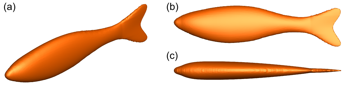
Figure 2: Three-dimensional fish geometry based on a giant danio.

The parameter $a_{0}$ determines the amplitude of the deformation $h_{0}$ at the trailing edge. It is adjusted through a feedback control loop to ensure that the average net drag on the foil is $0$, as described in Appendix B. $h_{0}(x,t)$ can be used without the recoil and steering terms in order to prescribe the full kinematics of the swimmer, in which case $h(x,t)=h_{0}(x,t)$. For a freely moving body with prescribed deformation, the recoil is computed from the hydrodynamic forces on the body. In the latter case, the envelope of the actual displacement is given by $g(x)$, with peak to peak amplitude at the trailing edge given by $a=2g(1)$.

The prescribed kinematics of a carangiform swimmer, based on the experimental observation of steadily swimming saithe (Videler & Hess, 1984; Videler, 1993), is often modeled as:

$$a_{0}=0.1,\quad A(x)=1-0.825(x-1)+1.625(x^{2}-1),\quad\lambda=1,\quad B(x,t)=0.$$ (4)

This motion is for example used in Borazjani & Sotiropoulos (2008); Dong & Lu (2007) and, in the rest of the paper, will be referred to as the carangiform gait. Experimental observations of American eels (Tytell & Lauder, 2004) provide that anguilliform motion can be represented by:

$$a_{0}=0.1,\quad A(x)=1+0.323(x-1)+0.310(x^{2}-1),\quad\lambda=1,\quad B(x,t)=0.$$ (5)

Figure 3(a) shows the prescribed envelope $A(x)$ for the carangiform (resp. anguilliform) swimmer defined in equation 4 (resp. equation 5). Figure 3(b) illustrates the resulting mid-line displacement in the presence of the recoil term.

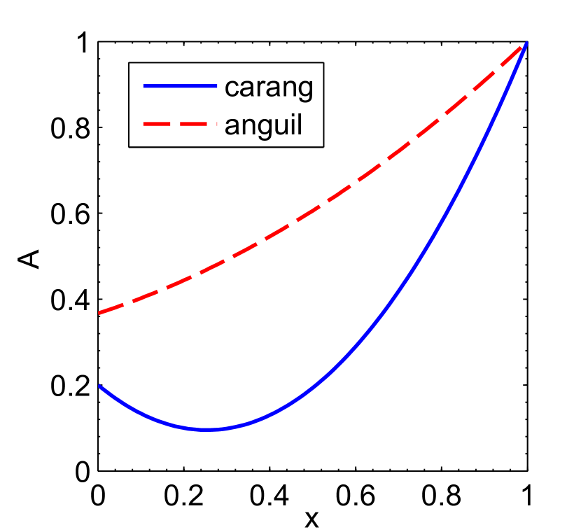
(a) Prescribed amplitude envelopes

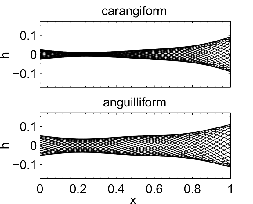
(b) Mid-line displacement

Figure 3: Carangiform and anguilliform motion for $f=1.8$ and $a_{0}=0.1$ at Reynolds number $\mbox{{Re}}=5000$ with recoil.

2.2 Kinematic parameters

The goal of this paper is to identify kinematic parameters that minimize the self-propelled swimming power $P_{in}$ for a given speed (Reynolds number) and body shape. In order to quantify the fitness of each motion, the quasi-propulsive efficiency $\eta_{QP}$ is used, which compares $P_{in}$ to the useful power, i.e. the resistance $R$ of the rigid-straight towed body at the same speed $U_{s}$ times the speed: $\eta_{QP}=RU_{s}/\overline{P_{in}}$. Indeed, as discussed in Maertens et al. (2015), the Froude propulsive efficiency is not appropriate here as it is zero for a self-propelled body.

For rigid flapping foils, the parameters that characterize the motion and its performance have been extensively studied (Anderson et al., 1998; Read et al., 2003)). The principal kinematic parameters are the Strouhal number and the maximum nominal angle of attack, and, to a lesser degree, the heave amplitude to chord ratio, and the phase angle between heave and pitch; all, typically, measured at $25\%$ of the chord. The Strouhal number is a wake parameter, since it characterizes the dynamics of the (unstable) wake (Triantafyllou et al., 1991, 1993); hence the width of the wake must, in principle, be used as the characteristic length. However, the width of the wake is unavailable beforehand, so this characteristic length is approximated typically by the peak to peak motion of the trailing edge. Hence, for an undulating flexible foil, we define the Strouhal number, heave amplitude, pitch angle and nominal angle of attack at the trailing edge. These parameters and others used throughout this paper are summarized in table 1. While the motion cannot be characterized by these parameters alone, they play an important role in determining the swimming efficiency. Changing the amplitude of motion and Strouhal number can be achieved through parameters like $a_{0}$ and $f$ (though, for a given motion and average velocity, there is a unique amplitude that ensures a steady velocity), but the pitch amplitude $\theta_{\max}$ and maximum angle of attack $\alpha_{\max}$ cannot be directly controlled. Therefore, when optimizing the swimming gait, it is important to choose a parametrization that allows to adjust the pitch and angle of attack amplitudes independently of the heave amplitude and Strouhal number. This is best done by changing parameters that control the derivative of the prescribed envelope $A(x)$ at the trailing edge.

In this study, the lateral flexing motion (i.e. the lateral motion after the linear and angular recoil are subtracted) is characterized by four parameters: the frequency, amplitude, and two parameters controlling the shape of $A(x)$, the envelope of the unsteady bending motion. With prescribed frequency, the amplitude is adjusted to ensure self-propulsion, while the two remaining parameters are varied systematically in order to identify the values that minimize the swimming power (equivalently, maximize the quasi-propulsive efficiency $\eta_{QP}$) for a given Reynolds number and body flexing shape. In order to explore a wide range of motions, two different parametrizations are used for $A(x)$: a quadratic envelope and a Gaussian envelope (see details in § 3.1). The wavelength of the traveling wave is fixed, equal to the body length, and the maximum amplitude is adjusted to ensure the average swimming speed of the self-propelled fish results in Reynolds number $\mbox{{Re}}=5000$. The linear and angular recoil terms are computed by integration of the hydrodynamic forces.

Name	Symbol	Expression
Power coefficient	$C_{P}$	$2P_{in}/(\rho U_{s}^{3}L)$
Quasi-propulsive efficiency	$\eta_{QP}$	$RU_{s}/\overline{P_{in}}$
Reynolds number	Re	$U_{s}L/\nu$
Strouhal number	$St$	$fa/U_{s}$
Pitch angle	$\theta$
Angle of attack	$\alpha$
Peak to peak heave	$a$
heave-pitch phase angle	$\psi$

Table 1: Kinematic and other dimensionless parameters.

2.3 Governing equations and numerical implementation

In a self-propelled swimming body, its motion is determined by the coupled fluid-body dynamics. The physical parameters are non-dimensionalized by the fish body length $L$, its intended average cruising speed $U_{s}$, and the density of water $\rho$.

In order to solve the coupled fluid/body problem described above, we adapted the 2nd order boundary data immersion method (BDIM) presented in Maertens & Weymouth (2015). The validation of the numerical method presented in this section for simulating self-propelled undulating bodies is presented in Appendix A. For the two-dimensional simulations, constant velocity $\vec{u}=\vec{U}_{s}$ is used on the inlet ($x=-6$), periodic boundary conditions on the upper and lower boundaries ($y=\pm 2.4$), and a zero gradient exit condition with global flux correction ($x=7$). The Cartesian grid is uniform near the fish with grid size $\,\mathrm{d}x=\,\mathrm{d}y=1/160$ and uses a $2\%$ geometric expansion ratio for the spacing in the far-field, as illustrated in figure 4. The three-dimensional simulations are run on a $6\times 3\times 3$ domain with constant velocity $\vec{u}=\vec{U}_{s}$ on the inlet, a zero gradient exit condition with with global flux correction and periodic boundary conditions along $y$ and $z$ boundaries. The Cartesian grid is uniform near the fish with grid size $\,\mathrm{d}x=\,\mathrm{d}y=\,\mathrm{d}z=1/100$ and uses a $4\%$ geometric expansion ratio for the spacing in the far-field.

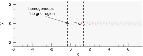
Figure 4: Flow configuration for the undulating NACA0012 simulations. The vorticity field for the carangiform motion with $f=1.8$ and zero mean drag is shown as an example.

The fluid and body equations are integrated over the fluid and body domains, respectively, $\Omega_{f}$ and $\Omega_{b}$, with a kernel of radius $\epsilon=2\,\mathrm{d}x$. The BDIM equations for the smoothed velocity field $\vec{u}_{\epsilon}$ are valid over the complete domain $\Omega=\Omega_{f}\cup\Omega_{b}$ and enforce the no-slip boundary condition at the interface. These equations, integrated from time $t$ to time $t_{+}=t+\Delta t$, are:

$$\vec{u}_{\epsilon}(t_{+})=\;\vec{v}(t_{+})+\left(\mu_{0}^{\epsilon}(d)+\mu_{1}^{\epsilon}(d)\frac{\partial}{\partial n}\right)\big{(}\vec{u}_{\epsilon}(t)-\vec{v}(t_{+})+\vec{R}_{\Delta t}-\vec{\partial P}_{\Delta t}\big{)}$$ (6a)

$$\vec{\nabla}\cdot\vec{u}_{\epsilon}(t_{+})=0$$ (6b)

where $\vec{v}$ is the velocity field associated with the closest body, $\hat{n}$ the unitary normal to the closest fluid/solid boundary (pointing toward the fluid), and $d$ the signed distance to the closest boundary ($d>0$ within the fluid, $d<0$ inside a body). $\mu_{0}^{\epsilon}$ and $\mu_{1}^{\epsilon}$ are respectively the zeroth and first central moments of the smooth delta kernel (see Maertens & Weymouth (2015) for more details). The pressure impulse $\vec{\partial P}_{\Delta t}$ and $\vec{R}_{\Delta t}$ accounting for all the non-pressure terms are defined as:

$$\vec{R}_{\Delta t}(\vec{u})=\int_{t_{0}}^{t_{0}+\Delta t}\left[-\left(\vec{u}\cdot\vec{\nabla}\right)\vec{u}+\nu\nabla^{2}\vec{u}\right]\ \text{d}t\text{ ,}\qquad\vec{\partial P}_{\Delta t}=\int_{t_{0}}^{t_{0}+\Delta t}\frac{1}{\rho}\vec{\nabla}p\ \text{d}t.$$ (7)

In order to simplify the equations of motion, we consider motion within the $(x,\,y)$ plane, such that the translational velocity of the body center of mass (COM), $\vec{v}_{c}$, is a two-dimensional vector $(v_{c}^{x},\,v_{c}^{y})$, and its rotation velocity is $\omega_{b}=\omega_{b}^{z}$. We then define the generalized velocity $\boldsymbol{V}$, location $\boldsymbol{X}$, and force $\boldsymbol{F}$ vectors, as well as the generalized mass matrix $\mathbf{M}$:

$$\boldsymbol{V}=\begin{pmatrix}v_{c}^{x}\\ v_{c}^{y}\\ \omega_{b}\end{pmatrix},\quad\boldsymbol{X}=\frac{\text{d}\boldsymbol{V}}{\text{d}t},\quad\boldsymbol{F}=\begin{pmatrix}F^{x}_{h}\\ F^{y}_{h}\\ M_{c}^{z}\end{pmatrix},\quad\mathbf{M}=\begin{pmatrix}m&0&0\\ 0&m&0\\ 0&0&I_{c}\end{pmatrix},$$ (8)

where $\vec{F}_{h}$ is the hydrodynamic force on the body, $m$ is the mass of the body which has density $\rho_{b}=\rho$ and $I_{c}$ its moment of inertia with respect to the COM. The motion of the body is governed by:

$$\frac{\text{d}}{\text{d}t}\left(\mathbf{M}\boldsymbol{V}\right)=\boldsymbol{F}.$$ (9)

The coupled dynamic equations are discretized using a sequentially staggered Euler explicit integration scheme with Heun’s corrector. Sequentially staggered schemes are computationally efficient, but for large added mass they become unconditionally unstable (Förster et al., 2007), regardless of the particular scheme used. In order to stabilize the numerical scheme, we introduce the virtual added mass matrix $\mathbf{M_{a}}$.

The virtual added mass, which is used in an implicit added mass scheme (Connell & Yue, 2007; Zhu & Shoele, 2008; Peng & Zhu, 2009), can eliminate the instability due to large added mass, but its exact value will not affect the results. In the case of an undulating fish, the coefficients of the matrix can be estimated from the added mass of the fish at zero angle of attack, or heuristically tuned to avoid instability. In the present simulations, the virtual added mass is a diagonal matrix with value $[0\ 11m\ 13m]$.

We also define the total mass as:

$$\mathbf{M_{T}}=\mathbf{M}+\mathbf{M_{a}}.$$ (10)

With these new definitions, we integrate equation 9 over a time-step $\Delta t$ in the form:

$$\boldsymbol{V}(t+\Delta t)=\boldsymbol{V}(t)+\mathbf{M_{T}}^{-1}\int_{t}^{t+\Delta t}\left[\boldsymbol{F}+\mathbf{M_{a}}\frac{\text{d}\boldsymbol{V}}{\text{d}\tau}\right]\text{d}\tau.$$ (11)

At each time step $t_{n}$, the fluid and body velocities, $\vec{u}_{n}=\vec{u}_{\epsilon}(t_{n})$ and $\vec{v}_{n}=\vec{v}(t_{n})$ respectively, are calculated from the velocities and forces at the previous time steps according to equations 6 and 11.

2.4 The importance of recoil

Equation 11 determines the recoil $B(x,t)$ resulting from the prescribed motion $h_{0}(x,t)$ and the related hydrodynamic forces $\boldsymbol{F}$. Due to the significant added complexity incurred by the recoil term, most of the earlier simulation studies neglected it (Borazjani & Sotiropoulos, 2008; Dong & Lu, 2007). However, the amplitude of this term, and its impact on the estimated swimming power are substantial (Reid et al., 2012), as illustrated below.

We consider first the carangiform motion of Eq. 4 with frequency $f=2.1$. Figure 5(a) shows the dimensionless linear and angular momentum for the self-propelled fish, including the recoil, as determined by the hydrodynamic forces and adaptive amplitude $a_{0}$. The angular and transverse momentum are larger than the longitudinal momentum, but the three amplitudes are comparable. However, the non-dimensional moment of inertia of the fish is much smaller than its mass:

$$m=0.081,\,\qquad I_{c}=0.0045,$$ (12)

where the mass and moment of inertia are non-dimensionalized by the length $L$ and density $\rho$. Therefore, whereas the linear momentum results in velocities smaller than $3\%$ of the free-stream $U_{s}$, the rotation of the fish generates velocities at the trailing edge up to $40\%$ of the free-stream, as shown in Figure 5(b). This observation suggests that, whereas the longitudinal motion of the fish might be negligible, the transverse motion, and specifically the motion due to the free-rotation, are important.

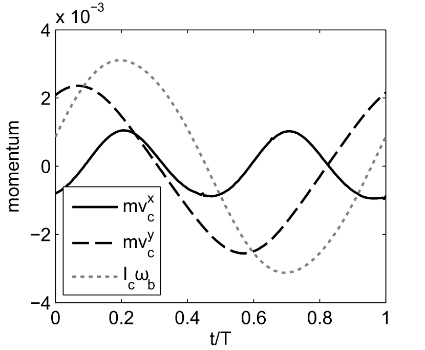
(a) Linear and angular momentum

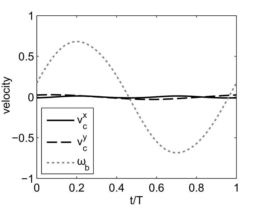
(b) Velocity and rotation rate

Figure 5: (a) Linear and angular momentum and (b) corresponding velocities for a neutrally buoyant self-propelled NACA0012 with carangiform motion at frequency $f=1/T=2.1$.

In order to further illustrate this result, figure 6 shows the quasi-propulsive efficiency as a function of frequency for the carangiform and anguilliform motions with and without recoil. The figure shows that, at all frequencies, the undulation with recoil requires more power than the undulation without recoil. Therefore, simulations that do not allow for recoil are likely to underestimate the swimming power, as discussed in Reid et al. (2009). The figure also shows that the optimal frequency without recoil might differ from the optimal frequency with recoil. In the cases studied here, the optimal frequency for the carangiform undulation without recoil is around $f=1.6$, while with recoil it is around $f=2.1$.

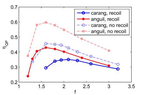
Figure 6: Quasi-propulsive efficiency as a function of frequency for the carangiform and anguilliform motions with and without recoil.

In summary, we have shown here that the impact of the pitch motion of the fish on swimming performance is significant. In order to estimate meaningful values of fish swimming efficiency, it is critical to allow for recoil.

2.5 Gait optimization procedure

Eloy (2013) and Tokić & Yue (2012) combined an evolutionary algorithm with Lighthill’s potential flow slender-body model to simultaneously optimize the shape and kinematics, using, respectively, $22$ and $9$ parameters. In this paper we employ viscous simulations that are far more demanding computationally, hence we parameterize the amplitude $A(x)$ using only two parameters, because the small number of parameters allows us to find an optimum with a reduced number of evaluations, and it also facilitates the visualization and interpretation of the results.

For a given kinematic parametrization and frequency, the envelope $A(x)$ is optimized using derivative-free optimization (Rios & Sahinidis, 2013). We apply the BOBYQA algorithm that performs bound-constrained optimization using an iteratively constructed quadratic approximation for the objective function (Powell, 2009). For each set of parameters, the viscous simulation is run for $15$ non-dimensional time units, and the average power coefficient $\overline{C_{P}}$ across the last $10$ undulation periods is calculated. Based on the values of $\overline{C_{P}}$, the implementation of BOBYQA provided by the NLopt free C library (Johnson, n.d.) interfaced with Matlab computes the next set of parameters. In order to avoid finding a local minimum due to numerical noise, after the algorithm has converged, it is run again using the previously found minimum as a starting point.

3 Efficiency of swimming in open-water

The goal in this section is to identify undulatory gaits that require the minimum amount of power ($\overline{P_{in}}$) to drive an elongated body at speed $U_{s}$, such that the Reynolds number is $\mbox{{Re}}=5000$. In other words, we want to maximize the quasi-propulsive efficiency $\eta_{QP}$ of the self-propelled undulating body and identify the key parameters under the constraints of fixed body size and shape, as well as Reynolds number. We first consider a two-dimensional NACA0012-shaped fish and then apply the results to a three-dimensional danio-shaped body.

3.1 Gait optimization for a two-dimensional foil

For several values of undulation frequency, we optimize the deformation envelope $A(x)$. $A(x)$ has been traditionally modeled by a quadratic function, of the form:

$$A(x)=1+c_{1}(x-1)+c_{2}(x^{2}-1).$$ (13)

In the figures we parametrize each envelope by $A(0)$ and $A(1/2)$, the envelope amplitude at the leading edge and mid-chord respectively (the amplitude at the trailing edge being constrained to $A(1)=1$). Indeed, $A(0)$ and $A(1/2)$ are more meaningful than $c_{1}$ and $c_{2}$ and can easily be restricted to a rectangle. First, we fix the undulation frequency to $f=1.8$ and optimize the quadratic envelope $A(x)$, restricting $A(0)$ to positive values. Figure 7a shows the efficiency as a function of $A(0)$ and $A(1/2)$. The carangiform envelope used in previous sections is denoted by a black square, and the anguilliform gait through a diamond. It is clear that the envelopes above the dashed line, which are concave envelopes with a peak upstream from the trailing edge, have good efficiency. The efficiency decreases very quickly below the dashed line, as the envelope becomes convex with an increasing amplitude at the trailing edge. Therefore, the envelope traditionally used to model carangiform swimming is inefficient, whereas the anguilliform envelope, which is closer to a straight line, is much more efficient. Among the concave envelopes, $A(0)=0$ seems best, together with $1\leq A(1/2)\leq 1.7$, where the efficiency reaches a value of $48\%$. Since the optimal quadratic gait saturates the constraint $A(0)\geq 0$, we then fix the leading edge amplitude to $A(0)=0$ and optimize the undulation frequency $f$ and the second envelope parameter $A(1/2)$. Figure 7b shows the efficiency as a function of $f$ and $A(1/2)$. Here again, around the optimal point, the efficiency is not very sensitive to the exact value of $f$ and $A(1/2)$. The optimal quadratic envelope ($A(0)=0$, $A(1/2)=1$, $A(1)=1$) has a maximum amplitude at $x=3/4$ and reaches an efficiency of $\eta_{QP}=49\%$ around $f=1.6$.

Figure 7: $\eta_{QP}$ as a function of $A(0)$ or $f$ and $A(1/2)$ for quadratic envelopes. The black dots show the location of the points that have been used to build the thin-plate smoothing spline ($\mathsf{tpaps}$ function in Matlab with smoothing parameter $p=0.999$) represented in color. (a): fixed frequency $f=1.8$. The carangiform and anguilliform motions are respectively denoted by a black square and a black diamond, and a dashed line shows the location of linear envelopes (points below this line correspond to convex envelopes, while above it the envelopes are concave). (b): fixed leading edge value $A(0)=0$.

A quadratic envelope has been traditionally used to describe the displacement envelope of undulating fish which is maximum at the trailing edge, but the envelope of the curvature amplitude in saithe and mackerel has a distinctive peak around the peduncle section Videler & Hess (1984). The results from figure 7 also suggest that the efficiency is higher if the deformation is largest upstream of the trailing edge rather than at the trailing edge itself. Such envelopes can be better modeled by a Gaussian function of the form:

$$A(x)=\exp\left({-\left(\frac{x-x_{1}}{\delta}\right)^{2}+\left(\frac{1-x_{1}}{\delta}\right)^{2}}\right),$$ (14)

where $x_{1}$ parametrizes the location of the peak and $\delta$ its width, as shown in figure 8. With the Gaussian function, it is easy to change the pitch and angle of attack amplitudes at the tail by adjusting the location and width of the peak. Since the Gaussian envelope is always positive, the entire $(x_{1},\,\delta)$ space can be used to search for an optimal gait without running into degenerate gaits.

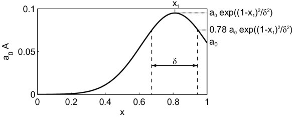
Figure 8: Definition of the parameters for a Gaussian envelope.

Figure 9 shows the efficiency as a function of $x_{1}$ and $\delta$ in the neighborhood of the optimal envelope for $\lambda=1$ and five frequencies ranging from $f=1.5$ to $f=2.7$. For all frequencies, the efficiency decreases very rapidly as $\delta$ is decreased below its optimal value, while the efficiency is much less sensitive to increases above this optimal value. Moreover, while for all frequencies it is possible to find a region in the $(x_{1},\,\delta)$ space that reaches an efficiency of $50\%$ (see table 2(a) for details), the optimal envelope clearly depends on the frequency.

Figure 9: $\eta_{QP}$ as a function of $x_{1}$ and $\delta$ near the optimum for Gaussian envelopes. (a): $f=1.5$, (b): $f=1.8$, (c): $f=2.1$, (d): $f=2.4$, (e): $f=2.7$, (f): colorbar. The black dots show the location of the points that have been used to build the thin-plate smoothing spline ($\mathsf{tpaps}$ function in Matlab with smoothing parameter $p=0.999$) represented in color.

At low frequency, gaits with undulations of the entire body ($x_{1}=0.73$ and $\delta=0.52$ at $f=1.5$) are most efficient, while at high frequency, the undulations should be restricted to a narrow region ($\delta=0.21$ at $f=2.7$) located around $25\%$ of the trailing edge ($x_{1}=0.88$ at $f=2.7$). However, for all frequencies, the optimized deformation envelope $A(x)$, shown in figure 10a, is qualitatively similar to the curvature envelope from Videler & Hess (1984), with a small amplitude at the leading edge, a peak $10$ to $30\%$ from the trailing edge, and a sharp decrease in amplitude at the trailing edge. Moreover, for all frequencies, the amplitude of the peak is very close to $0.1$.

The corresponding displacement envelopes $g(x)$ are shown in figure 10b. The displacement envelopes are qualitatively similar to the carangiform displacement envelope from Videler & Hess (1984), with a minimum amplitude around $x=0.25$ and a maximum amplitude at the trailing edge. While the amplitude at the leading edge decreases by a factor of two from $f=1.5$ to $f=1.8$, it remains almost constant for $f$ from $2.1$ to $2.7$ with a value $g(0)=0.02$ very close to that of Videler & Hess (1984).

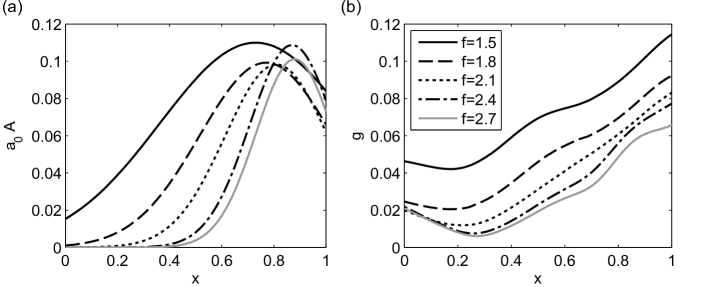
Figure 10: Optimized (a) prescribed deformation envelopes and (b) displacement envelopes for the Gaussian parametrization. $\lambda=1$ and $f=[1.5,\,1.8,\,2.1,\,2.4,\,2.7]$.

It is interesting to note that, since quadratic envelopes can only result in functions with a wide peak, they can reach the same efficiency as the wide peak Gaussian envelopes at low frequency ($f=1.5$), but not at high frequency ($f=2$) where a sharp peak is advantageous.

3.2 Characterization of efficient swimming gaits for a two-dimensional fish

We showed in the previous section that, by changing the location and width of the peak in a Gaussian deformation envelope, a very efficient gait can be designed for a large range of undulation frequencies.

Figure 11 shows the deformed fish for three optimized gaits. As expected from figure 10, at $f=1.5$ the entire length of the fish undergoes noticeable deformation and displacement, resulting in a swimming motion that is similar to that of an anguilliform swimmer, with a moderate curvature along the entire body: the deformation of the fish matches the large wavelength trajectory of the trailing edge and thus avoids the efficiency loss associated with a large angle of attack. At higher frequency, the front half of the fish undergoes virtually no deformation, resulting in a swimming motion very similar to a carangiform ($f=2.1$) or even a thuniform ($f=2.7$) swimmer. At this frequency, the region that would correspond to the peduncle deforms with a very large curvature caused by the sharp peak in the Gaussian envelope. This allows the deformation of the fish to match the small wavelength trajectory of the trailing edge and thus avoid the efficiency loss associated with a large angle of attack.

Figure 11: Superimposed body outlines over one undulation period for three frequencies.

Figure 12 shows the deformed fish and vorticity snapshots for the five optimized gaits at $t/T=0\ (\text{mod }1)$, where $T=1/f$ is the undulation period. With a Gaussian deformation envelope, a peak width specifically tailored to the undulation frequency allows for reduced angle of attack at all frequencies. This helps the boundary layer remain attached, as previously observed for waves traveling faster than the free stream (Taneda, 1977; Shen et al., 2003). As for thrust-producing flapping foils, a reverse Kármán vortex street forms in the wake. The width and wavelength of the reverse Kármán vortex street decreases with increasing undulation frequency, and secondary small vortices develop at low frequency.

Figure 12: Snapshots of vorticity for optimized gaits at $t/T=0\ (\text{mod }1)$. (a): $f=1.5$, (b): $f=1.8$, (c): $f=2.1$, (d): $f=2.4$, (e): $f=2.7$, (f): colorbar.

Table 2(a) summarizes the parameters and properties of the five optimized gaits. The quasi-propulsive efficiency $\eta_{QP}$ of these undulatory gaits is of prime interest. The efficiency reaches $57\%$ for $f=2.7$, whereas the least efficient frequency, $f=1.5$ reaches $\eta_{QP}=49\%$. An other important parameter is the Strouhal number, which is close to $St=0.35$. The consistency of the Strouhal number for the optimized envelopes across frequencies suggests that, for a given Reynolds number, there exists an optimal Strouhal number that can be reached with a large range of frequencies. Like the Strouhal number, the maximum pitch angle $\theta_{\max}$ and maximum angle of attack $\alpha_{\max}$ are almost constant across the five optimized gaits, with a value close to $\theta_{\max}=31^{\circ}$ and $\alpha_{\max}=17^{\circ}$. The corresponding phase angle between the heave and pitch of the trailing edge is $\psi=82^{\circ}$. The results from this optimization show that, as in rigid flapping foils, the efficiency of undulating fish is primarily driven by the Strouhal number, angle of attack, heave motion (or pitch motion), and heave-pitch phase angle, all at the trailing edge. The optimal Strouhal number, pitch angle, and angle of attack can be attained by tuning the envelope peak for each frequency.

$f$	$x_{1}$	$\delta$	$a_{0}$	$a$	$\theta_{\max}(^{\circ})$	$\alpha_{\max}(^{\circ})$	$\psi(^{\circ})$	$St$	$\overline{C_{P}}$	$\eta_{QP}$
$1.5$	$0.73$	$0.52$	$0.084$	$0.23$	$31$	$17$	$82$	$0.34$	$0.093$	$0.49$
$1.8$	$0.77$	$0.36$	$0.066$	$0.18$	$28$	$19$	$82$	$0.33$	$0.089$	$0.52$
$2.1$	$0.81$	$0.28$	$0.062$	$0.16$	$29$	$20$	$81$	$0.35$	$0.087$	$0.53$
$2.4$	$0.87$	$0.23$	$0.079$	$0.15$	$35$	$16$	$82$	$0.37$	$0.083$	$0.56$
$2.7$	$0.88$	$0.21$	$0.073$	$0.13$	$34$	$15$	$84$	$0.36$	$0.081$	$0.57$

(a) Optimized envelopes at several frequencies.

$f$	$x_{1}$	$\delta$	$a_{0}$	$a$	$\theta_{\max}(^{\circ})$	$\alpha_{\max}(^{\circ})$	$\psi(^{\circ})$	$St$	$\overline{C_{P}}$	$\eta_{QP}$
$1.8$	$0.65$	$0.50$	$0.050$	$0.17$	$22$	$22$	$82$	$0.30$	$0.097$	$0.45$
$1.8$	$0.78$	$0.49$	$0.068$	$0.18$	$26$	$21$	$78$	$0.32$	$0.093$	$0.47$
$1.8$	$0.80$	$0.29$	$0.082$	$0.22$	$36$	$17$	$84$	$0.40$	$0.096$	$0.46$
$1.8$	$0.85$	$0.31$	$0.101$	$0.22$	$37$	$16$	$82$	$0.40$	$0.095$	$0.46$
$1.8$	$0.90$	$0.37$	$0.103$	$0.21$	$35$	$19$	$78$	$0.38$	$0.094$	$0.46$
$1.8$	$0.90$	$0.25$	$0.186$	$0.32$	$53$	$10$	$87$	$0.57$	$0.140$	$0.31$

(b) Examples of envelopes around the optimal gait at $f=1.8$.

Table 2: Parameters and properties of gaits with Gaussian envelopes. Motion parameters are the frequency $f$, peak location $x_{1}$, peak width $\delta$ and amplitude $a_{0}$. Properties are the peak to peak displacement amplitude at the trailing edge $a$, maximum pitch angle at the trailing edge $\theta_{\max}$, maximum angle of attack $\alpha_{\max}$, heave and pitch phase angle $\psi$, Strouhal number $St$, time-averaged power coefficient $\overline{C_{P}}$ and the quasi-propulsive efficiency $\eta_{QP}$.

In order to better understand the impact of $x_{1}$ and $\delta$ on the gait properties, table 2(b) summarizes these properties for several values of $x_{1}$ and $\delta$ near the optimum for $f=1.8$. As the location of the peak moves aft and its width decreases, the portion of the fish undergoing significant deformation reduces, therefore a larger amplitude is necessary to ensure that enough thrust is produced. As a result, the Strouhal number and maximum pitch angle increase. This observation also allows us to interpret the optimization results. For a fixed envelope $A(x)$, the Strouhal number of a self-propelled undulating fish increases with decreasing frequency. In order to mitigate this effect, an envelope with widespread undulations (small $x_{1}$ and large $\delta$) that can produce the same thrust with smaller amplitude makes it possible to reach the optimal Strouhal number even at low frequency. Similarly, at high Reynolds number, a large $x_{1}$ and a small $\delta$ make it possible to generate the required thrust at the optimal Strouhal number. When the undulation frequency reaches about $2.5$, the optimal envelope parameters reach a plateau at $x_{1}\approx 0.9$ and $\delta\approx 0.2$.

Figure 13 shows the pressure field and body velocity for the optimized envelopes with frequency $f=[1.5,\,2.1,\,2.7]$ at their respective time of minimum and maximum power. For $f=1.5$ (figures 13a,b) and $f=2.7$ (figures 13e,f), there are three distinct sections along the upper side of the fish: high pressure near the leading edge, low pressure in the middle and high pressure near the trailing edge (and the opposite on the other side). In figures 13b,f, these sections almost exactly match transverse velocity of respectively positive, negative, and positive sign, resulting in very large instantaneous swimming power. Conversely, in figures 13a,e, the sign of the transverse velocity is reversed, resulting in a significant negative swimming power. For $f=2.1$, the pressure changes along the fish are smaller, and the pressure is close to zero along a large portion of the fish. Moreover, unlike for $f=2.7$, the sign changes in pressure do not match the sign changes in transverse velocity. For instance, at $t/T=0$, the pressure along the bottom side of the fish near the trailing edge is positive (not shown here), which would result in a positive swimming power. Therefore, the minimum power is reached at a later time $t/T=0.12$, at which point the amplitude is largest in areas where the pressure is close to zero, resulting in a very small power. Similarly, the maximum power reached at $t/T=0.34$ is not as large as for $f=2.7$ because the sections of high pressure do not exactly match the sections of large transverse velocity.

It must be pointed out that there are additional parameters affecting the efficiency of an undulating fish, since the efficiency ranges from $\eta_{QP}=0.49$ at $f=1.5$ to $\eta_{QP}=0.57$ at $f=2.7$. Shen et al. (2003) found that a slip ratio around $s_{r}=0.8$ ($f=1.2$) is optimal for a body undergoing traveling wave motion of constant amplitude, in order to reduce separation effects and turbulence intensity. In our case, however, these results do not strictly apply because the undulations have a non-constant envelope, and especially for higher frequency are confined to a small section of the fish.

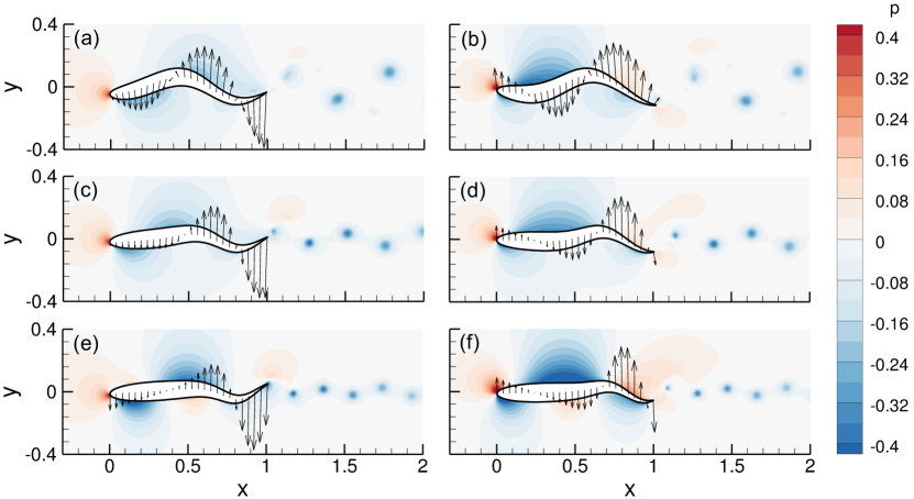
Figure 13: Snapshots of pressure field with arrows showing the body velocity. (a, b): optimized Gaussian envelope at $f=1.5$; (c, d): optimized Gaussian envelope at $f=2.1$; (e, f): optimized Gaussian envelope at $f=2.7$. (a, c): $t/T=0.12\ (\text{mod }1)$ (minimum power for $f=1.5$ and $f=2.1$); (e): $t/T=0\ (\text{mod }1)$ (minimum power for $f=2.7$); (b, d): $t/T=0.34\ (\text{mod }1)$ (maximum power for $f=1.5$ and $f=2.1$; (f): $t/T=0.29\ (\text{mod }1)$ (maximum power for $f=2.7$).

3.3 Application to a three-dimensional danio-shaped swimmer

We have so far modeled a fish by a two-dimensional fish-like flexible foil. However, fish have a highly three-dimensional geometry. In particular, most carangiform and thunniform swimmers are characterized by a region of reduced depth, around $20\%$ from the trailing edge, the peduncle. In order to model this region of reduced added mass with a two-dimensional geometry, it might be more appropriate to model a fish with a separate foil for the tail, as illustrated in figure 14. The fish model shown in this figure undulates with the optimized gait at frequency $f=2.4$ identified earlier, and the performance ($\eta_{QP}=0.54$) is very close to that obtained with a single foil, indicating that the results are robust to changes in the geometry.

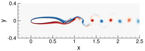
Figure 14: Snapshot of the vorticity field around a two-dimensional fish with a separate tail fin.

In the rest of this section, we consider a simplified three-dimensional fish shape, shown in figure 2, which is based on a giant danio (Devario aequipinnatu). For this geometry, we fix the undulation frequency to $f=2.4$ and optimize a Gaussian envelope for quasi-propulsive efficiency (for a fixed swimming speed $U_{s}$, we minimize the expanded power $\overline{P_{in}}$). In figure 15 we compare how $\eta_{QP}$ changes with the envelope parameters $x_{1}$ and $\delta$ for a two-dimensional fish and for the three-dimensional shape. The efficiency is generally lower with the three-dimensional shape, but the dependence on $x_{1}$ and $\delta$ is very similar for both geometries: the most efficient gaits are for $0.8<x_{1}<0.9$ and $0.2<\delta<0.3$ with a sharp decrease in efficiency for $\delta<0.2$. This shows that, even though three-dimensional effects reduce the swimming efficiency, most of the conclusions about BCF swimming drawn from the two-dimensional study extend to three-dimensional shapes.

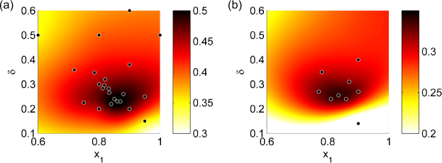
Figure 15: $\eta_{QP}$ as a function of $x_{1}$ and $\delta$ near the optimum for (a) $2D$ and (b) $3D$ geometries with $f=2.4$. The black dots show the location of the points that have been used to build the thin-plate smoothing spline ($\mathsf{tpaps}$ function in Matlab with smoothing parameter $p=0.999$) represented in color.

The parameters and properties of the optimized gait for $f=2.4$ are compared to those of the carangiform gait in table 3. Like in the 2D case, the optimization decreases the power consumption by $50\%$ compared with the carangiform gait. As in 2D, the optimized gait manages to bring the phase angle between the heave and pitch motion of the trailing edge close to $90^{\circ}$, which significantly reduces the angle of attack. As a result, the optimized gait for the three-dimensional fish shape have a pitch angle, phase angle and angle of attack very close to the optimized gait for the two-dimensional fish. However, since the 3D effects reduce the thrust produced by the undulating motion, the Strouhal number is higher than in 2D, especially for the carangiform gait.

$f$	$x_{1}$	$\delta$	$a_{0}$	$a$	$\theta_{\max}(^{\circ})$	$\alpha_{\max}(^{\circ})$	$\psi(^{\circ})$	$St$	$\overline{C_{P}}$	$\eta_{QP}$
$3.0$	carangiform		$0.099$	$0.18$	$34$	$41$	$59$	$0.53$	$0.035$	$0.22$
$2.4$	$0.84$	$0.26$	$0.085$	$0.18$	$37$	$17$	$87$	$0.43$	$0.023$	$0.34$

Table 3: Parameters and properties of 3D undulating gaits. Properties are the peak to peak displacement amplitude at the trailing edge $a$, maximum pitch angle at the trailing edge $\theta_{\max}$, maximum angle of attack $\alpha_{\max}$, heave and pitch phase angle $\psi$, Strouhal number $St$, time-averaged power coefficient $\overline{C_{P}}$, and the quasi-propulsive efficiency $\eta_{QP}$. The optimized gait at $f=2.4$ is compared to the carangiform gait at $f=3$.

Figure 16 shows the deformation envelope $A(x)$ and the displacement envelope $g(x)$ for the carangiform gait at $f=3$ and for the optimized gait. The superimposed body outlines for the optimized gait shown in figure 17b also look very similar to the body outlines of the optimized motions in 2D: the deformation of the tail follows the trajectory of the trailing edge, resulting in an efficient low angle of attack. The body outlines for the carangiform motion, on the other hand, show that the pitch of the tail is out of phase with its velocity (phase angle far from $90^{\circ}$), which results in a very inefficient gait, with a large angle of attack.

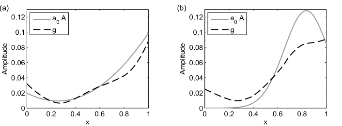
Figure 16: Prescribed deformation envelope $a_{0}A(x)$ and displacement envelope $g(x)$ for (a) carangiform gait with $f=3$ and (b) optimized gait with $f=2.4$.

Finally, we show the flow structure around the 3D fish model for both gaits in figure 18. The performance difference between the two gaits is accompanied by noticeable differences in the wake structure of the two swimmers. For both gaits, figures 18a and 18b show wakes comprised of two interconnected vortex loops per cycle, together with other smaller structures. In particular, the structure in the wake of the optimized motion is complex, with many vortex tubes interlaced with each other. Indeed, as can also be seen in the vorticity field at $z=0$ (figure 18d), the deformation at the peduncle is quite large for the optimized gait, resulting in vortex tubes separating from the main body and then interacting with the structures shed from the tail.

Figure 17: Superimposed body outlines over one undulation period for (a) the carangiform motion and (b) the optimized gait.

Borazjani & Sotiropoulos (2010) also observed in their 3D simulations that, for Strouhal number greater than $St=0.3$, the wake structure observed in 2D, dominated by a single vortex pair (or ring in 3D), transitions to vortex loops wrapping around each other. Dong et al. (2006) showed that the same phenomenon happens to elliptical flapping foils of finite aspect ratio: at low aspect ratio/large Strouhal number, two vortex rings are shed each cycle. As the aspect ratio increases or the Strouhal number decreases, the tip vortices do not merge together any more and the wake consists of interconnected loops. As the Strouhal number further decreases or the aspect ratio increases, the three-dimensional effects become even weaker and the linkage between tip vortices disappears. At this point, the 3D wake looks similar to the (reverse) Kármán vortex street observed in 2D.

In the carangiform example shown here, the tip vortices merge, while with the optimized gait, which has a lower Strouhal number and angle of attack, they do not. At higher Reynolds number, the Strouhal number would be smaller and a wake similar to that observed in 2D would probably emerge. Figure 18c,d shows that, near the tail, the vorticity in the $z=0$ plane looks very similar to that behind a 2D foil. However, under the influence of the tip vortices, the vortex sheets shed by the tail do not evolve into two strong vortices as in 2D. As a result, whereas the pressure field around the undulating fish-like shape is very similar to the pressure around an undulating airfoil, the pressure signature in the wake shown at the plane $z=0$ is very weak (18e,f). However, the pressure signature in the plane $z=0.06$, just above the peduncle is much stronger (18g,h).

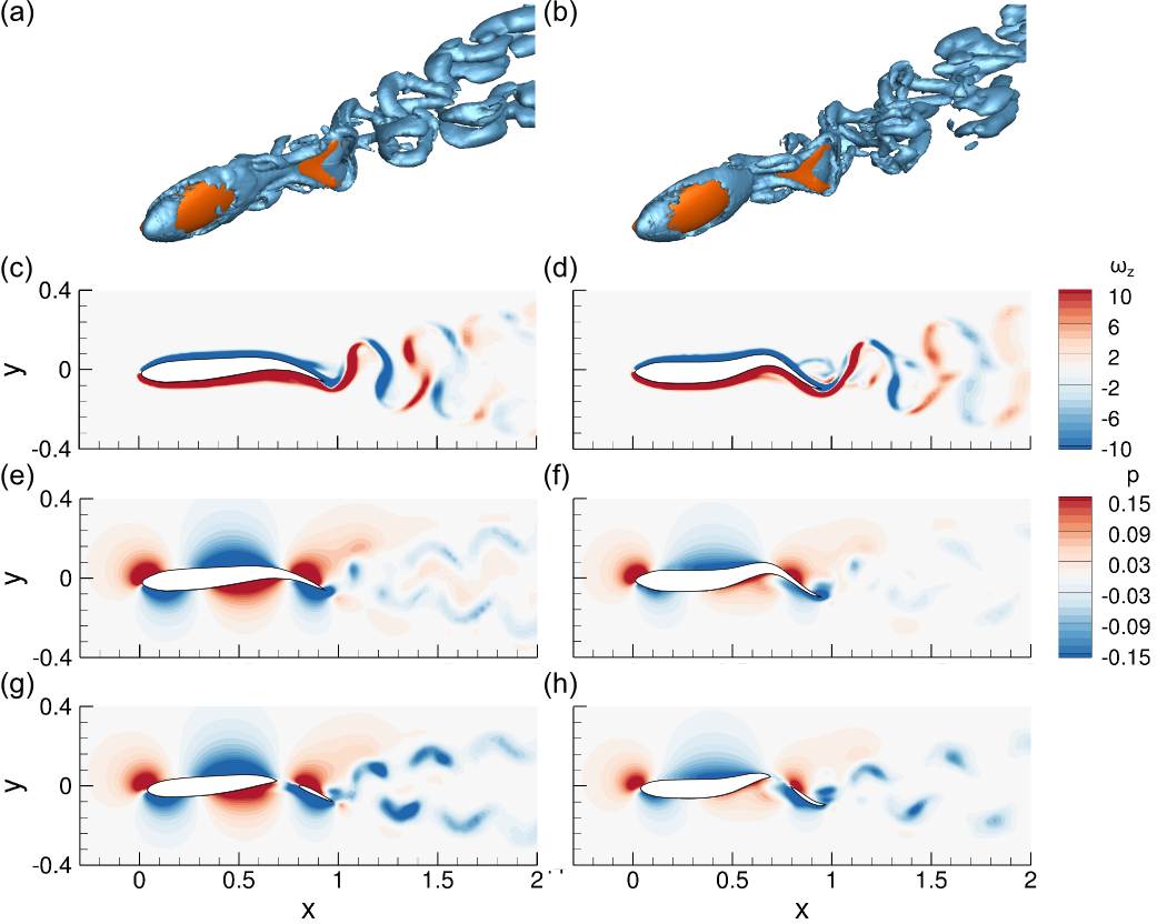
Figure 18: Snapshots of the flow around a three-dimensional fish with (a,c,e,f) a carangiform and (b,d,g,h) an optimized gait . (a,b): Three-dimensional vortical structures visualized using the $\lambda_{2}$-criterion; (c,d): $z$ component of the vorticity in the $z=0$ plane; (e,f): pressure in the $z=0$ plane; (g,h): pressure in the $z=0.06$ plane.

Figure 19 shows a magnified view of the vortex structures generated by the carangiform motion. A red line shows the formation of a clear vortex ring at the trailing edge of the tail between figures 19a and 19c. In figure 19e, the vortex ring is fully formed and detached from the tail. Since the vortex rings are oblique, they produce a large transverse velocity, which is inefficient and results in waste of energy. We also see a spanwise narrowing of the vortex rings as they convect downstream, as also observed in the simulations of Blondeaux et al. (2005) and Dong et al. (2006) for a respectively rectangular and elliptical pitching and heaving foil.

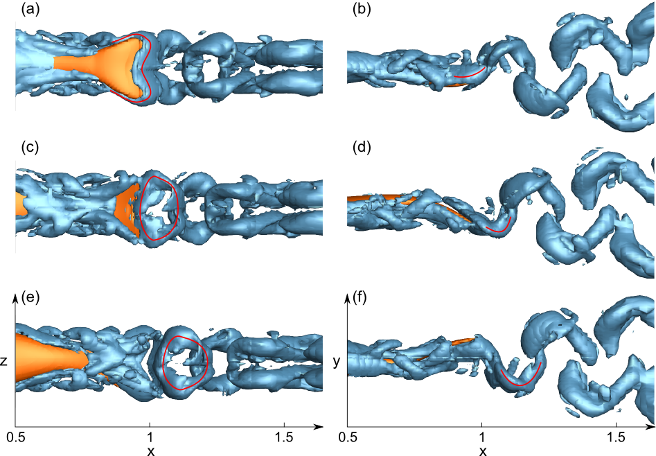
Figure 19: (a,c,e) Side-view and (b,d,f) top-view of the vortex structures at several time-steps for the carangiform gait. (a,b): $t/T=0.1\ (\text{mod }1)$; (c,d): $t/T=0.4\ (\text{mod }1)$; (e,f): $t/T=0.7\ (\text{mod }1)$. A red line shows the formation of a vortex ring.

Figure 20 shows a magnified view of the vortex structures generated by the optimized gait. The structure of the wake is more intricate than for the carangiform motion. In particular, instead of one set of interconnected vortex tubes, there are two sets of tubes, marked in red and green in the figure. The loop marked in red is the same as observed for the carangiform gait, but at this lower Strouhal number, it never fully closes into a clearly defined vortex ring. The tubes marked in green are formed upstream of the tail and are shed from the body as a result of the large curvature at the peduncle. The resulting vortex tubes are interlaced with the vortex loops from the tail with which they have a phase difference of close to $180^{\circ}$.

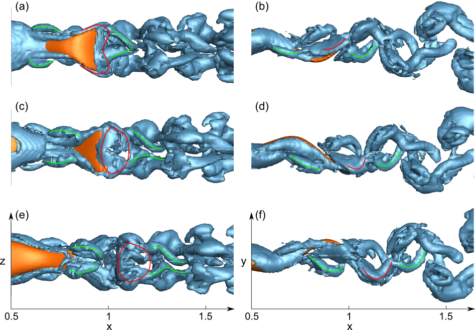
Figure 20: (a,c,e) Side-view and (b,d,f) top-view of the vortex structures at several time-steps for the optimized gait. (a,b): $t/T=0.1\ (\text{mod }1$; (c,d): $t/T=0.4\ (\text{mod }1$; (e,f): $t/T=0.7\ (\text{mod }1$. A red line shows a vortex shed from the tail that never fully develops into a ring, while green lines show the vortices shed from the body.

For a three-dimensional fish shape with two-dimensional undulation, as for a two-dimensional foil, the Strouhal number, pitch angle (or heave motion), nominal angle of attack and phase angle at the trailing edge are the key parameters for efficient swimming. The optimization results in a lower Strouhal number and angle of attack, which reduces the three-dimensional effects observed behind the non-optimized gait, such as formation of inefficient oblique vortex ring chains. With the optimized gait, the production of thrust is also distributed between the body and the tail, which shedd vortex structures with opposite phase. It has been shown with turbines, for instance, that distributing the thrust production (or energy capture) could significantly improve the efficiency, and it is possible that fish use the same process. Finally, while we used a simplified fish geometry with a two-dimensional undulation, fish can also rely on three-dimensional motion of their dorsal and pectoral fins to save energy (Lauder & Madden, 2007; Drucker & Lauder, 2001).

4 Energy saving in two fish swimming in close proximity

The experimental study by Gopalkrishnan et al. (1994) and the theoretical study by Streitlien et al. (1996) demonstrated that flapping rigid foils placed within a Kármán street can extract significant energy from the flow through vorticity control. Subsequently, it was documented that live fish swimming within a Kármán vortex street formed behind a cylinder tend to synchronize their motion to the oncoming cylinder vortices. This allows them to significantly reduce the energy spent to hold station (Liao et al., 2003b, a; Akanyeti & Liao, 2013), or even generate propulsive force with no input power as evidenced by the passive propulsion of anaesthesized fish (Beal et al., 2006). The phenomenon of fish Kármán gaiting has been explained by the faculty of fish to sense and harness the energy of the vortices.

Since a foil or a fish can extract energy from the vortices in a Kármán street, in principle there is no reason why they could not extract energy from the vortices in a reverse Kármán street. Boschitsch et al. (2014) recently showed that the net propulsive efficiency of a pitching foil located behind a similarly pitching foil could be anywhere between $0.5$ and $1.5$ times that of an isolated foil, depending on the phase. This indicates that the energy extracted from the vortices in a reverse Kármán street more than compensates for the effect of increased drag caused by the jet forming in a reverse Kármán street (unlike the energetically beneficial drag wake forming behind a bluff body). Despite the strong evidence that it is possible to harness the energy of individual vortices within a reverse Kármán street, there is no conclusive evidence that fish actually do harness this energy. Liao summarizes in his review of fish swimming in altered flows that “no hydrodynamic or physiological data exist to evaluate the hypothesis that fish can increase swimming performance by taking advantage of the wake of other members” (Liao, 2007).

Due to the difficulty of experimentally measuring the swimming power of individual fish in a school, simulations can provide valuable information to help clarify this issue. Hence, we consider next a pair of undulating fish-like foils. We have shown in the previous section that a two-dimensional fish, undulating in open-water, can attain a quasi-propulsive efficiency of almost $60\%$ by optimizing its gait. The goal in this section is to determine whether, by working as a pair, fish can further reduce the power required to travel at constant speed $U_{s}$.

4.1 Flow in the wake of a self-propelled undulating fish

The flow in the wake of a self-propelled undulating fish consists of vortices of alternating sign. The vorticity snapshot in figure 21a shows that the vortices decrease in strength under the effect of diffusion, but this is a slow process and the wake is primarily characterized by its periodicity. Figure 21b shows that the vortices are arranged in such a way that the flow along the $y=0$ axis is faster than the ambient flow (jet-like flow), whereas the flow away from the centerline moves slower than the ambient flow; consistent with the momentum-less wake, on average, of a self-propelled body (Triantafyllou et al., 1993). As a result, the time-averaged vorticity field in figure 21c is characterized by four shear layers of alternating sign, resulting in a jet along the centerline with strips of slowed-down flow on either side, as shown in figure 21d.

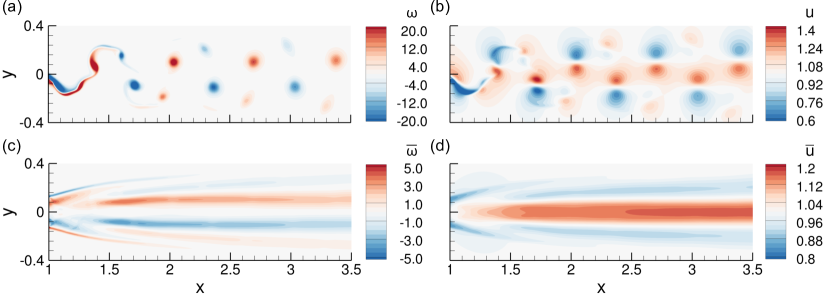
Figure 21: Wake behind a self-propelled undulating fish for the optimized gait with Gaussian envelope and $\lambda=1$ at frequency $f=1.5$. (a): instantaneous vorticity field; (b): instantaneous $x$-velocity field; (c): time-averaged vorticity field; (d): time-averaged $x$-velocity field.

The reverse Kármán vortex street behind a self-propelled undulating fish is characterized by its periodic structure with vortices moving parallel to the $y=0$ axis in stable formation. The vorticity at longitudinal distance $d$ from the trailing edge in the wake of an undulating fish can be modeled as:

$$\omega(d,y,t)=\omega_{y}(y,t)\,\omega_{d}(d)\sin\big{(}2\pi\left(\phi_{1}(d)-ft\right)\big{)},\qquad\phi_{1}(d)=d/\lambda_{w}+\phi_{w},$$ (15)

where the frequency $f$ is given by the undulation frequency and the wavelength $\lambda_{w}$ and phase $\phi_{w}$ of the wake need to be determined. For the five optimized gaits with Gaussian envelope and $\lambda=1$ presented in § 3.1, we estimated from the vorticity field the phase $\phi_{1}$ at several distances $d$ along the wake. In figure 22a we show the phase $\phi_{1}$ as a function of the distance $d$, as well as the least squares linear fit for each swimming gait. The coefficients for the linear fit are summarized in table 4. For all the gaits, the phase is essentially proportional to the distance $d$, with a coefficient of proportionality very close to the undulation frequency $f$. Since $\lambda_{w}=fc_{w}$, where $c_{w}$ is the speed at which the vortices travel in the wake, this result shows that the vortices travel at the same speed as the free-stream. Moreover, for the five gaits considered, the phase at $d=0$ is around $0.25$, which means that the vortices are shed by the fish when the trailing edge has maximum transverse velocity. Finally, we confirm these observations by plotting $\phi_{1}$ as a function of $fd$ in figure 22b. Assuming $c_{w}=1$, the least-squares estimate ($\pm$ standard deviation) of the phase $\phi_{w}$ is:

$$\phi_{w}=0.24\pm 0.02.$$ (16)

From now on, $\lambda_{w}=1/f$ and $\phi_{w}=0.25$ will be used to estimate the phase $\phi_{1}$ encountered by a downstream fish whose leading edge is located at distance $d$ from the upstream fish.

Figure 22: Vorticity phase in the wake of self-propelled undulating fish as a function of (a) distance and (b) distance times frequency. For each frequency, the optimized gait with Gaussian envelope is used.

Gait parameters			$\phi_{1}$ linear fit		$c_{w}=1$
$f$	$x_{1}$	$\delta$	$1/\lambda_{w}$	$\phi_{w}$	$\phi_{1}-fd$
$1.5$	$0.73$	$0.52$	$1.52$	$0.19$	$0.22$
$1.8$	$0.77$	$0.36$	$1.77$	$0.26$	$0.24$
$2.1$	$0.81$	$0.28$	$2.07$	$0.30$	$0.26$
$2.4$	$0.87$	$0.23$	$2.37$	$0.29$	$0.26$
$2.7$	$0.88$	$0.21$	$2.65$	$0.29$	$0.25$

Table 4: Parameters of the gaits used in the wake vorticity phase estimate and fitted phase and wavelength for the vorticity in the wake. An estimate of the phase $\phi_{w}$ assuming a phase speed $c_{w}=\lambda_{w}/f=1$ is also provided.

Whereas the pressure signature in the wake shown at the plane $z=0$ is very weak (18e,f), the pressure signature in the plane $z=0.06$, just above the peduncle is much stronger (18g,h), and could still be used by a downstream fish to reduce its swimming energy.

4.2 Effect of phase and distance for two fish in-line

Here we consider two fish-like foils following each other and undulating at frequency $f=1.5$ with the optimized gait for this frequency, as illustrated in figure 24. The amplitude of undulation, $a_{0}$, is adjusted independently for each fish to ensure that both fish are in a stable position and produce zero net thrust on average. We vary the distance $d$ between the trailing edge of the upstream fish and the leading edge of the downstream fish, as well as $\phi$, the phase of the downstream fish motion as defined in Eq. 2.1. An important parameter will be $\Delta\phi$, the phase difference between the motion of the downstream fish leading edge and the vortices it encounters: $\Delta\phi=\phi-\phi_{1}(d)$. In order to measure the impact of the pair configuration on each fish, we define $R(C_{P})$ (resp. $R(a_{0})$), the ratio of the power coefficient (resp. amplitude) in the pair configuration over the power coefficient (resp. amplitude) for the corresponding gait in open water.

Both fish can benefit from swimming in pair, but the trends are very different. The swimming power and amplitude of the upstream fish is virtually independent of the phase of the downstream fish, as shown in figure 23a. For large separations $d$, the downstream fish does not impact the upstream fish whose efficiency is then almost the same as in open-water. However, as the downstream fish gets close ($d<0.5$), the high pressure around the leading edge of the downstream fish ‘pushes’ the upstream foil, regardless of their phase difference. As a result, the upstream fish can reduce its swimming amplitude, expending less power than it would in open-water. At $d=0.25$, the undulation amplitude is reduced by $10\%$, resulting in $28\%$ energy saving, corresponding to a quasi-propulsive efficiency (based on the towed drag on open-water) of $\eta_{QP}=69\%$.

Figure 23: Time-averaged power coefficient $\overline{C_{P}}$ and amplitude $a_{0}$ for (a) the upstream fish as a function of ditance $d$ and (b) the downstream fish as a function of phase $\Delta\phi$. The solid (resp. dashed) line marks the average value with respect to the phase (resp. distance) and the shaded area indicates the range of values reached across the various distances (resp. phases).

For the downstream fish, the situation is very different. Even when the upstream fish is several chord lengths ahead, the downstream fish encounters its wake. The performance of the downstream fish is determined by its interaction with the vortices of the wake. It appears from 23b that the swimming power of the downstream fish depends primarily on the phase difference $\Delta\phi$ between its undulation and the encountered vortices. Regardless of the distance $d$, the swimming power of the downstream fish is low if $\Delta\phi$ is between $0.7$ and $1$, and it is high if $\Delta\phi$ is between $0.1$ and $0.5$. Like for the upstream fish, the reduced swimming power results from a reduced undulation amplitude $a_{0}$, but despite a more significant reduction in amplitude ($27\%$ for $\Delta\phi=0.8$), the power reduction does not exceed that of the upstream fish. For the downstream fish, a maximum energy saving of $24\%$ is reached at $\Delta\phi=0.85$, corresponding to an efficiency of $\eta_{QP}=65\%$.

Figure 24 shows the vorticity field around the two fish undulating with frequency $f=1.5$ at distance $d=1$ for the phase $\Delta\phi=0.83$ that minimizes the swimming power of the downstream fish. At $t/T-\phi=0.25$, the downstream fish approaches the negative vortex (at $x=-0.1$ on its left) as it is turning its “head” (leading edge) to the right. This acceleration of the head causes a low pressure on the left side of the head, as shown in figure 25e. Due to its position, the approaching negative vortex causes an increase in the longitudinal velocity, as shown in figure 25b, which results in an increased stagnation pressure (figure 25f). However, this vortex also generates a large transverse velocity with negative sign, as shown in figure 25d. As a result, the effects of the head motion are amplified by the incoming vortex, displacing the stagnation point downstream on the right side and deepening the low pressure on the left side (figure 25f). While the energy required by the fish to rotate its head is increased, the drag is decreased, despite the faster flow encountered by the fish.

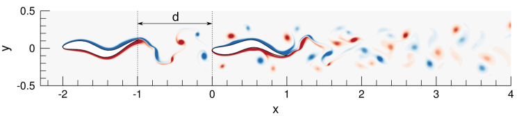
Figure 24: Snapshot of the vorticity field for two fish undulating at $f=1.5$ with separation distance $d=1$ and optimal phase $\Delta\phi=0.83$ at time $t/T-\phi=0.25\ (\text{mod }1)$. The color axis is the same as in figure 12.

At the same time, the positive vortex located at $x=0.2$ on the right side of the fish thickens the boundary layer and significantly accelerates the flow in a region where the fish undulation already accelerates it (figure 25a,b). This interaction between the vortex and the fish results in a very large pressure drop around $x=0.3$ that also contributes to the reduction in drag while increasing the swimming power. The vortices are convected downstream at a speed which is substantially lower than the phase speed of the fish deformation. Further downstream, the distance between the vortices and the fish increases, and their interaction becomes weaker. At the trailing edge, the phase between the vortices and the fish motion is close to $\pi$, such that the positive vortex reaches $x=1$ as the trailing edge of the fish is at its leftmost position. This vortex will be shed just upstream of the same sign vortex shed by the downstream fish. The resulting wake configuration is unstable and it takes several body lengths for the wake to reorganize into two pairs of opposite sign vortices per cycle.

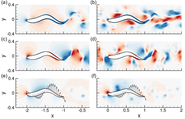
Figure 25: Snapshot of the velocity and pressure field for two fish undulating at $f=1.5$ with separation $d=1$ and optimal phase $\Delta\phi=0.83$. (a,b) $x$-velocity; (c,d): $y$-velocity; (e,f): pressure and arrows showing the velocity of the fish. (a,c,e): upstream fish at $t/T=0.25\ (\text{mod }1)$; (b,d,f): downstream fish at $t/T-\phi=0.25\ (\text{mod }1)$. The same color axis as in figure 13 is used for the pressure, and the same as in figure 21b is used for the velocity (centered in $0$ for the $y$-velocity).

The results presented in this section are consistent with the experimental results from thrust producing rigid pitching foils in an in-line configuration (Boschitsch et al., 2014). We found that for small separation distance the propulsive efficiency of the upstream fish is greatly improved. We also showed that the efficiency of the downstream fish only weakly depends on the separation distance, the primary parameter being the phase difference between the wake from the upstream fish and the undulating motion of the downstream fish. If the undulation amplitude was fixed, the downstream fish would experience an increased drag and decreased power for $0\leq\Delta\phi\leq 0.5$, whereas it would experience a decreased drag and increase power for $0.5\leq\Delta\phi\leq 1$. For a self-propelled fish, the energetic benefits of a reduced amplitude resulting from a reduced drag overcome the power increase caused by the vortices.

4.3 Effect of frequency for two undulating fish in-line

Next, we fix the distance between the two fish to $d=1$ and vary their undulation frequency. For frequencies $f=[1.5,\,1.8,\,2.1]$, their optimized Gaussian envelope is used, for which the parameters are summarized in table 4. Figure 26 shows that most of the conclusions drawn in § 4.2 still hold as the undulation frequency is increased. While the upstream fish is mostly unaffected by the presence and phase of the downstream fish, the undulation amplitude of the downstream fish is largest for $0\leq\Delta\phi\leq 0.5$ and smallest for $0.5\leq\Delta\phi\leq 1$. However, the correlation between amplitude and power coefficient is not as strong any more, and the exact value of the optimal phase depends on the frequency. For instance, at $f=2.1$, the amplitude is minimum for $\Delta\phi=0.85$, but the power coefficient is minimum for $\Delta\phi=0$. Whereas with $f=1.5$ most phases result in an increased amplitude and power coefficient, with $f=1.8$ and $f=2.1$, the amplitude and power coefficient of the downstream fish never exceed that of the upstream fish. Therefore, at these frequencies, it is always beneficial to swim in the wake of an undulating fish, despite the increased average velocity of the encountered flow.

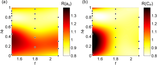
Figure 26: Ratio of (a) amplitude and (b) power coefficient as a function of frequency $f$ and phase $\Delta\phi$ for two fish swimming in-line at distance $d=1$. The ratios are defined with respect to the corresponding gait in open water. The black dots show the location of the points that have been used to build the thin-plate smoothing spline ($\mathsf{tpaps}$ function in Matlab with smoothing parameter $p=0.999$) represented in color.

At frequency $f=1.8$, the results for the optimal phase, shown in figure 27, are very similar to those described in the previous section for $f=1.5$, with the vortices from the upstream fish reinforcing the effect of the body undulation. However, the wake at this frequency is narrower; therefore the vortices are closer to the fish and they lose more strength through their interaction with the boundary layer. Moreover, since the distance between two consecutive vortices is proportional to the undulation frequency, the vortices are spaced closer to each other. The resulting wake is dominated by two single vortices shed by the downstream fish, each accompanied by weaker vortices of opposite sign from the upstream fish. This is identical to the destructive vortex interaction mode of a flapping foil within a Kármán street in Gopalkrishnan et al. (1994), which has been associated with increased efficiency.

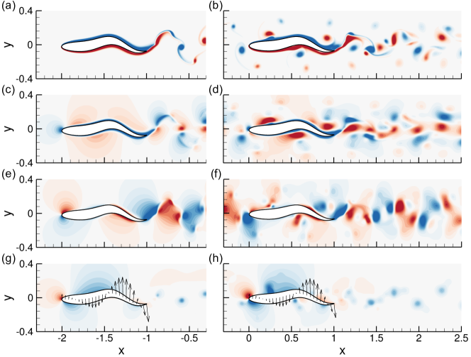
Figure 27: Snapshot of the vorticity, velocity and pressure field for two fish undulating at $f=1.8$ with separation distance $d=1$ and optimal phase $\Delta\phi=0.87$. (a,b) vorticity; (c,d) $x$-velocity; (e,f): $y$-velocity; (g,h): pressure and arrows showing the velocity of the fish. (a,c,e,g): upstream fish at $t/T=0.25\ (\text{mod }1)$; (b,d,f,h): downstream fish at $t/T-\phi=0.25\ (\text{mod }1)$. The same color axis as in figure 13 is used for the pressure, and the same as in figures 21a and b for vorticity and velocity (centered in $0$ for the $y$-velocity).

Figure 28 illustrates the cases of the downstream fish undulating with the phase providing the worse swimming efficiency for $f=1.8$. In this configuration, the vortices from the upstream fish counteract the effects of the undulating motion of the downstream fish. As the fish turns its head to the right, displacing the stagnation point to the right and causing a low pressure on the left side of the head, the positive $y$-velocity caused by the approaching positive vortex has the opposite effect. The high velocity regions caused by the vortices along the fish correspond to low velocity regions from the undulating motion. Finally, when the vortices from the upstream fish reach the trailing edge, they merge with the same sign vortices from the downstream fish. The resulting wake is very stable and is a classical reverse Kármán vortex street much wider than the one behind a single fish. This corresponds precisely to the constructive interaction mode of a flapping foil within a Kármán street in Gopalkrishnan et al. (1994), which has been shown to have reduced efficiency.

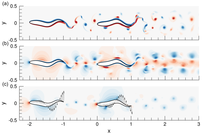
Figure 28: Snapshots of (a) vorticity, and (b) pressure field for two fish undulating at $f=1.8$ with separation distance $d=1$ and phase $\Delta\phi=0.38$ at $t/T-\phi=0.25\ (\text{mod }1)$. The same color axis as in figure 21a is used for the vorticity and the same as figure 13 for the pressure.

As the frequency increases further, the vortices from the upstream fish lose even more energy through interaction with the boundary layer of the downstream fish; therefore for each period of oscillation the wake behind the two fish contains a pair of single vortices, as shown in figure 29. Moreover, since the efficiency of the downstream fish mostly depends on the phase of the leading edge with respect to the arrival of the upstream fish reverse Kármán street vortices, the phase of the trailing edge with respect to the incoming vortices in the optimal configuration changes with frequency.

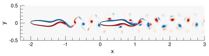
Figure 29: Snapshot of the vorticity field for two fish undulating at $f=2.1$ with separation distance $d=1$ and phase $\Delta\phi=0$. The same color axis is used as in figure 21a.

For all the frequencies considered here, a self-propelled fish can save energy by undulating behind another self-propelled fish undulating at the same frequency, reaching efficiencies close to $\eta_{QP}=70\%$. By properly phasing its motion with respect to the incoming vortex street, the vortices can reinforce the effect of the undulation. Whereas for a fixed amplitude this phase would result in an increased swimming power, the reduction in drag results in an overall decreased swimming power.

4.4 Fish undulating in the reduced velocity region of the wake

We have so far considered the case of a pair of fish swimming in an in-line configuration. Since our fish model has a feedback controller ensuring its stability in $y$, it is also possible to impose an asymmetric configuration with an offset in the $y$ direction. Indeed, according to Weihs’ theory (Weihs, 1973), the only way for a fish to save energy in a school is to swim in the region of reduced velocity located between two wakes. We have already shown that a fish can save energy by swimming directly in the wake of another self-propelled fish and will now investigate if additional savings are possible by swimming in areas of reduced flow velocity. Figure 21d shows that, even with a single fish upstream, the flow on either side of the wake is slower than the free stream: for $f=1.5$ the average flow is slowest at $y=\pm 0.17$. With the downstream fish offset from the upstream fish by $\Delta y=0.17$, we vary the phase difference $\Delta\phi$ in order to see if the downstream fish can also save energy when swimming at this location.

Figure 30 shows that, even when the downstream fish is offset from the vortex street, its swimming performance greatly varies with the phase. However, it is easier for the fish to save energy in this region of reduced flow velocity than directly behind the upstream fish. Directly behind the upstream fish, only $30\%$ of the phases result in energy savings, and by using the unsteadiness of the wake, the quasi-propulsive efficiency at $f=1.5$ can be brought up from $50\%$ to $60\%$. When undulating in the region of reduced flow velocity, it is easier to save energy since over $70\%$ of the phases result in energy savings. The energy savings can even be very large since $\eta_{QP}=80\%$ is possible for $\Delta\phi=0.65$.

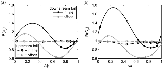
Figure 30: Ratio of undulation amplitude $a_{0}$ and time-averaged power coefficient $\overline{C_{P}}$ as a function of phase for two fish undulating at $f=1.5$ with longitudinal separation distance $d=1$. In-line fish and fish at an offset $\Delta y=0.17$ are compared.

Figure 31 shows that, at the optimal phase, the leading edge of the downstream fish reaches its leftmost position at the same time as it reaches a positive vortex. Figure 32b shows that the leading edge of the downstream fish exactly passes through the region where the longitudinal velocity is smallest. As a result, the stagnation pressure is greatly reduced (figure 32d). Moreover, the region of accelerated flow between the negative vortex and the fish ($x=0.4$) reinforces the accelerated region caused by the undulation, which we showed earlier is beneficial.

Figure 31: Snapshot of the vorticity field for two fish undulating at $f=1.5$ with longitudinal separation distance $d=1$, transverse separation $\Delta y=0.17$ and optimal phase $\Delta\phi=0.65$ at time $t/T-\phi=0.1\ (\text{mod }1)$. The color axis is the same as in figure 12.

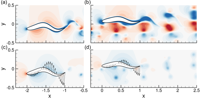
Figure 32: Snapshot of the (a,b) $x$-velocity and (c,d) pressure field for two fish undulating at $f=1.5$ with longitudinal separation distance $d=1$, transverse separation $dy=0.17$ and optimal phase $\Delta\phi=0.65$. (a,c): upstream fish, $t/T=0.1\ (\text{mod }1)$; (b,d): downstream fish, $t/T-\phi=0.1\ (\text{mod }1)$.The same color axis as in figure 13 is used for the pressure, and the same as in figure 21b for the velocity.

5 Discussion

5.1 Optimal BCF propulsion and the role of fish shape

It is interesting to note that, as the peak of the Gaussian describing the fish bending motion becomes sharper, the curvature imposed by the envelope in the peduncle section becomes much larger than the curvature caused by the traveling wave. This is particularly noticeable for $f=2.7$, at which frequency the undulations are mostly restricted to what would be the peduncle and tail sections for a fish.

The increase of the curvature in the peduncle region corresponding with a decreased stride length and increased swimming frequency is essential, allowing the instantaneous deformation of the fish to match the trailing edge trajectory (Figure 11). This serves to avoid the efficiency loss associated with a large angle of attack at the tail, as well as to keep the boundary layer attached to the fish. Indeed, the boundary layer remains attached to the fish as previously observed for waves traveling faster than the free stream (Taneda, 1977; Shen et al., 2003), and a reverse Kármán vortex street forms in the wake, consistent with previous studies of efficient thrust production in oscillating foils (Triantafyllou et al., 1991; Anderson et al., 1998). The width and wavelength of the reverse Kármán vortex street decreases with increasing undulation frequency, and secondary small vortices develop at low frequency.

The total lateral displacement of a live swimming fish is maximum at the trailing edge, but, once recoil is substracted, it becomes apparent that the body deformation is largest around the peduncle. We show that efficiency improves when the envelope of the body deformation is largest upstream of the trailing edge, because this creates a part of the body that is capable of acting as a caudal fin (and has roughly the length of the caudal fin). The high curvature of the peduncle region allows the (equivalent) caudal fin area to pitch independently from the motion of the body, in order to control the timing of trailing edge vortex shedding.

Fish employing the carangiform and thunniform swimming mode generally have a narrow peduncle, and our results suggest that there is function associated with this form. The narrow peduncle allows for sharp bending of the tail even at an angle with respect to the body deformation (providing a discontinuous slope), such as in the optimal motion at high frequency. Tunas, for example, have a special anatomy at the peduncle that allows powerful tendons to actuate the tail with substantial torque. This allows for the independent control of the tail in manipulating vorticity formed upstream of the tail along the body (Zhu et al., 2002), or from externally generated vortices. Wolfgang et al. (1999) demonstrated experimentally and numerically that high flexibility of the peduncle region allows for the caudal fin to precisely redirect vorticity shed upstream for optimal propulsion. In the 2D simulations conducted here the high curvature in the peduncle region serves the same purpose in allowing the fish shed vortices optimally.

Similar to (Borazjani & Sotiropoulos, 2010), we show that the optimal kinematics is mostly independent of body shape. Indeed, even a two-dimensional geometry can help assess the energetic performance of swimming kinematics.

5.2 Proposed schooling theory and comparison with Weihs’ theory

To our knowledge, the only existing hydrodynamic theory of schooling has been proposed by Weihs (1973). This theory provides useful insight based on time- averaged flow considerations, but does not factor in the potential benefits of energy extraction from the vortices. According to Weihs, a fish swimming directly behind another fish would experience higher relative velocity and would therefore have to spend extra energy. On the contrary, a fish swimming between two adjacent fish wakes would experience a reduced relative speed, allowing it to save energy. This strategy is known as flow refuging (Liao, 2007) or drafting.

As we have shown in this paper it is possible for a fish to save energy regardless of whether it swims directly behind another fish or at a lateral offset that allows it to benefit from a reduced flow velocity. The phase difference between its undulation and the wake vortices, $\Delta\phi$, determines whether its drag is reduced or enhanced. When swimming directly behind another fish, where the averaged flow is faster than the free-stream, the fish cannot save energy through drafting, and must therefore capture energy from individual vortices in order to save energy. We show that by using the transverse velocity of the individual vortices to amplify the pressure effects of the undulating motion, the fish can reduce its drag. Conversely, swimming in the region of the wake where the flow is, on average, slower, does not guarantee a reduced drag. However, we observed that it is possible to reduce drag and save energy by undulating in the region of reduced velocity than directly behind another fish, due to the possibility of taking advantage of both drafting and individual vortex energy capture. Up to 81% quasi-propulsive efficiency can be reached for a fish undulating with proper phase in the region of reduced flow velocity, compared with a maximum of 66% for a fish swimming directly behind another fish (Table 5).

$f$	$d$	$\Delta y$	$\Delta\phi$ (mod $1$)	$\eta_{QP}$(upstream)	$\eta_{QP}$(downstream)
$1.5$	$1$	$0$	$0.83$	$0.52$	$0.60$
$1.8$	$1$	$0$	$0.84$	$0.55$	$0.61$
$2.1$	$1$	$0$	$0.00$	$0.56$	$0.62$
$1.5$	$0.25$	$0$	$0.83$	$0.67$	$0.66$
$1.5$	$1$	$0.17$	$0.65$	$0.51$	$0.81$

Table 5: Efficiency for a pair of undulating fish in various advantageous configurations. The undulation frequency $f$, longitudinal separation $d$, transverse distance $\Delta y$ and the phase difference $\Delta\phi$ between the leading edge of the downstream fish and the vortices in the wake of the upstream fish are considered.

The energy contained in individual vortices can be harnessed in several ways. For a flapping foil in a Kármán vortex street, it is well known that the efficiency increases if the foil vortices destructively interact with the oncoming vortices, while the thrust can be enhanced if the foil vortices constructively interact with the oncoming vortices (Gopalkrishnan et al., 1994; Streitlien et al., 1996). For a fish swimming within a wake, constructive and destructive interaction can occur between the oncoming wake vortices and vortices emanating from the boundary layer of the fish, as well as between the wake vortices and the vortices shed at the fish’s trailing edge. Indeed, at the tail of the downstream fish, we observed that constructive interactions between the oncoming wake vortices and the vortices shed at the trailing edge were associated with reduced efficiency, while destructive interactions correlated with increased efficiency.

The interactions between the fish body and the oncoming vortices can result in enhanced thrust and/or improved efficiency. We show that the downstream fish can reduce its drag by consistently turning its head in a manner that employs the oncoming vortex flow to increase the transverse velocity across the head, amplifying the pressure field created at the head. While this increases the power consumed by the fish to rotate its head, the pressure drag at the head is decreased substantially to result in an overall improvement to the efficiency.

While reduced drag implies a reduced undulation amplitude for open-water self-propelled swimming, the correlation with energy saving is not as straightforward within a school, because the vortices impact both the drag and the swimming power. Since the quasi-propulsive efficiency is defined as $RU_{s}/\bar{P}_{in}$, the power consumed must be reduced for an increased efficiency. However, it can be directly or indirectly reduced. Directly, the power is reduced when vortices along the body of the fish exert force in the direction the fish is oscillating, thereby doing work on the fish. Indirectly, the vortices can help to reduce the overall drag on the fish, therefore reducing the amount of work the fish must perform to self-propel. If the undulation amplitude was kept constant, phases $0\leq\Delta\phi\leq 0.5$ would result in an increased drag and decreased power, and the reverse would apply to phases $0.5\leq\Delta\phi\leq 1$. The energy benefits of a reduced amplitude generally more than compensate for the increased swimming power, such that drag reduction tends to result in power reduction. However, the phase resulting in the smallest amplitude usually does not coincide with the optimal one. This suggests that multiple mechanisms are important for the efficiency of the downstream foil. In particular, the drag is mostly governed by the interaction between the head of the fish and the vortices, whereas the power is mostly governed by the interaction between these vortices and the tail, where the transverse velocities are much larger. The exact value of the optimal phase, therefore, depends on the undulation frequency and the gait.

In summary, a fish undulating in a vortex street cannot be considered as a rigid body with a propeller, located inside a jet. Regardless of the exact location of the fish in the vortex street, constructive interactions between the undulating body and the individual vortices can result in enhanced thrust, while destructive interactions result in increased swimming power. The exact value of the optimal phase depends on the gait details, but in general the drag reduction configurations are the most advantageous, and it is easier to reduce drag when undulating in a region of averaged reduced flow velocity, even in an asymmetric configuration.

6 Summary and Conclusions

We established through 2D and 3D numerical simulation the conditions for optimal propulsion in undulatory fish swimming, first for a single self-propelled fish, and then for a pair of identically shaped self-propelled fish moving in-line or at an offset, separated axially by a distance $d$.

First, we considered the problem of optimal propulsion of an undulating, self-propelled fish-like body, fully accounting for linear and angular recoil. We employed 2D simulations to conduct an extensive parametric search and then by employing targeted 3D simulations we established that properties found in 2D are qualitatively similar to those for 3D simulations.

In summary, the assumptions we employed in order to render the study feasible are:

1. Simulations were conducted at a Reynolds number of 5000.

2. For the 2D simulations, we modeled the fish body as an undulating NACA0012, while a danio-shaped body was used for 3D simulations. We model the main body of the fish and its caudal fin but not the other fins or details on the body such as other fins, finlets, eyes and other protrusions, and scales.

3. The motion of the fish consists of a steady axial translation at a prescribed speed, and a lateral body deformation in the form of a traveling wave of constant frequency $f$ and wavelength $\lambda=1$. Free axial rigid body motion as well as lateral and angular recoil were permitted and studied for their effect on propulsive efficiency.

4. The bending envelope was chosen to be either a quadratic or a Gaussian function of the length along the fish. For both functions, two parameters were sufficient to specify the shape of the envelope, with a third parameter $a_{0}$ to control the amplitude of the envelope. The total displacement envelope of live carangiform and anguilliform swimmers can be approximated by a quadratic function, but, after subtraction of the recoil, the envelope of body deformation is best approximated by a Gaussian function.

5. To maximize the quasi-propulsive efficiency (i.e. to minimize the energy expended), the two parameters used to specify the shape for each envelope (equations 3.1 and 3.2) were varied using an optimization scheme.

6. A PID controller adjusts the amplitude of oscillation $a_{0}$ until self-propulsion is obtained, and additionally maintains the heading of the fish by adjusting the camber.

The conclusions for optimal 2D swimming are as follows:

1. As with rigid flapping foils, the Strouhal number, phase angle between heave and pitch at the trailing edge, and nominal angle of attack are the principal parameters affecting the efficiency of propulsion.

2. Angular recoil has a significant impact on the efficiency of propulsion and hence must always be accounted for.

3. A Gaussian envelope enables a body deformation with high curvature in the region where the peduncle of the fish would be. This effectively allows the caudal fin to pitch independently with respect to the peduncle motion, and this extra degree of freedom allows for the control of flow patterns forming upstream of that position. Hence, whereas the convex profile traditionnaly used to model carangiform swimming provides quasi-propulsive efficiency of around 40%, an optimized profile results in efficiency of 57%.

For 3D swimming of a danio-shaped fish, which explicitly models the peduncle and caudal fin, the optimality conditions were observed to be very close qualitatively to those of 2D swimming, although the efficiency was consistently lower:

1. Angular recoil has significant impact on efficiency, as in 2D swimming.

2. Similarly to finite aspect ratio rigid flapping foils, the Strouhal number and maximum angle of attack are principal parameters affecting efficiency: For higher values of the Strouhal number the wake is also found to bifurcate, from a single row of connected vortex rings to a double row of vortex rings, resulting in reduced efficiency, as well as a complex three-dimensional structure in the wake. As expected, optimization reduces the Strouhal number to be closer to the optimal range, and hence the effect of wake bifurcation is also reduced. Within our parametric space, the Strouhal number was not reduced to values close to 2D swimming, and hence the effect of a bifurcating wake was not totally eliminated. It is expected that by, for example, increasing the span of the caudal fin, which reduces the required thrust coefficient, further increase in efficiency is possible.

3. The sharp curvature of the envelope of body deformation at the peduncle affects efficiency significantly. The efficiency increases from 22% for a convex imposed motion to 35% for an optimized body deformation with large deformation around the peduncle; both at Reynolds number 5000.

4. Heave and pitch motion at the trailing edge is close to $90^{\circ}$, as for a 2D swimming fish. The parametric dependence of the envelope shape is also qualitatively similar (Figure 16).

The resulting wake has a periodic 3D structure with coherent vortices that another fish can use to save energy by properly timing its motion. However, the three dimensional flow around a fish is far more complex than the flow around a two-dimensional flow. Since the three-dimensional effects mostly result in a loss of efficiency, the optimization reduces these effects while distributing the production of thrust between the body and the tail (resulting in $\eta_{QP}=34\%$).

Turning to the 2D swimming of two identical, self-propelled fish in close proximity, the geometric models and assumptions employed for a single fish optimization were used, under the following additional conditions: Both fish swim at the same speed and at a constant distance; the downstream fish is either directly behind the upstream fish, or at a lateral offset. The amplitude of motion of each fish is adjusted separately to achieve self-propulsion, and their kinematics are also optimized separately for expended energy. The power of each fish is compared with the power required when swimming alone. The following results are obtained:

1. The upstream fish may benefit from the mere presence of the downstream fish for very short relative distances. For example, a 28% energy saving at a distance of $d=0.25$ is achieved, but as the distance increases this is quickly reduced.

2. The downstream fish can benefit energetically even at axial distances equal to several times the body length, and in both the in-line position and in an offset position. This proves that energy saving is achieved through interaction with individual vortices as opposed to taking advantage of reduced oncoming flow (drafting), because in the in-line position the downstream fish is in a region of averaged increased relative velocity, which would be expected to cause an increase in drag.

3. The axial force on the downstream fish is mostly affected by the interaction between the head of the fish and the oncoming vortices, whereas the power required to sustain the undulating motion is affected by the interaction between these vortices and the body motion downstream from the head. The critical parameter for efficiency is the phasing between the head motion and the arrival of the vortices, since in general, a reduced drag results in a greater power reduction.

4. For the in-line arrangement, when fixing the relative distance to one body length, $d=1$, and varying the frequency, the efficiency of the downstream fish can increase to 66% for the optimal phase between the head motion and the arrival of the upstream fish vortices.

5. For the offset arrangement, at $\Delta y=0.17$, efficiency increases further, as the downstream fish also exploits the reduction in oncoming velocity. Still, an optimized phase is required, which makes it possible the reach a quasi-propulsive efficiency 81%, even though the fish can only interact with every other vortex produced by the upstream fish. It is expected that the efficiency of the downstream fish would increase further if there were two fish in the front, spaced by $\Delta y=0.34$ and perfectly synchronized.

6. Although the upstream fish vortices interact with the downstream fish over its entire length, as described above, it is remarkable that at the tail of the downstream fish the upstream and downstream fish vortices interact following the rules of Gopalkrishnan et al. (1994), viz. constructive interaction results in reduced efficiency, while destructive interaction provides increased efficiency.

Hence, we can conclude that swimming power can be reduced by swimming in a group for any position of the downstream fish; and for the upstream fish when positioned at close distances from the downstream fish. For the downstream fish, it can improve its thrust by interacting with oncoming vortices, and since reduced drag also reduces the power required to swim, this results in an increase of efficiency. On the contrary, bad timing leads to enhanced drag and swimming power. The schooling theory by Weihs (1973) predicts that a fish swimming directly behind another fish would experience increased drag and have to expend more power than in open-water. Wee show here that an additional consideration must be made on energy capture from the oncoming vortices, which depends on the phasing of the undulating motion with respect to the vortex street. When swimming in an offset location, energy savings can be maximized by simultaneously extracting energy from individual vortices and taking advantage of reduced oncoming flow velocity.

Appendix A Numerical method validation

Problems previously studied with BDIM include ship flows and flexible wavemaker flows (Weymouth et al., 2006), shedding of vorticity from a rapidly displaced foil (Wibawa et al., 2012), and a cephalopod-like deformable jet-propelled body (Weymouth & Triantafyllou, 2013). In Maertens & Weymouth (2015) we have demonstrated the ability of BDIM to handle several moving bodies and generalized the original method to accurately simulate the flow around streamlined foils at Reynolds numbers on the order of $\mbox{{Re}}=10^{4}$.

In order to validate the code for simulating undulating foils, the force and power resulting from a fully imposed kinematics are compared with results reported in the literature. Finally, a convergence study and sensitivity analysis on a self-propelled undulating foil are performed.

A.1 Undulating NACA0012 with fully imposed kinematics

Using a fully imposed carangiform undulation:

$$h(x,t)=\big{(}0.1-0.0825(x-1)+0.1625(x^{2}-1)\big{)}\sin\big{(}2\pi(x-ft)\big{)},$$ (17)

the undulation frequency is varied from $f=0.5$ to $f=2$ and the resulting time-averaged force and power coefficients are compared to the values from Dong & Lu (2007) in Figure 33. Note that in these simulations the kinematics is fully imposed, not allowing for recoil.

Figure 33: Time-averaged drag and power coefficients for an undulating NACA0012 as a function of frequency, compared with values from Dong & Lu (2007).

Similarly to Dong & Lu (2007), we find that the average power coefficient, slightly negative at $f=0.5$, increases to around $0.25$ at $f=2$, and that the drag is positive for $f<1.6$ and negative for $f>1.6$. The good agreement between our method and the results from Dong & Lu (2007) serves as a validation of the force and power calculation routines for an undulating foil.

A.2 Self-propelled undulating NACA0012

We now ensure that the simulation results presented here are independent of the grid parameters. In this section we consider the carangiform motion with frequency $f=2.1$.

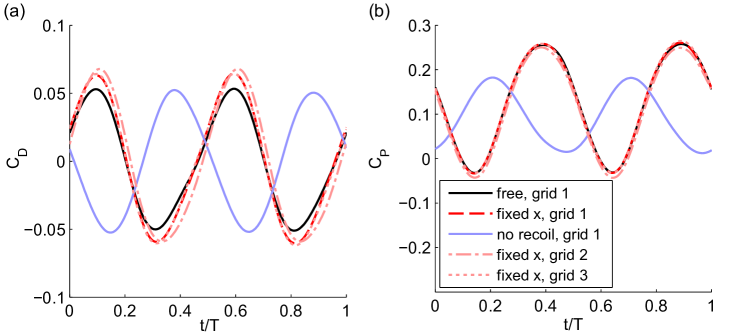
Figure 34: (a) Drag and (b) pressure coefficient on an undulating NACA0012 with carangiform motion at $f=1/T=2.1$. Various grids and constraints are compared. Grid $2$ is twice as fine as grid $1$, while the computational domain of grid $3$ is twice as large as that of grid $1$.

Figure 34 shows the evolution of power and drag coefficients during an undulation period $T$=1/f for various configurations. By comparing the free undulation and the fixed $x$ case, we first notice that fixing the $x$ location of the foil does not impact the power, confirming the observations from Bale et al. (2014). The amplitude of the drag oscillations are a bit larger for the case with fixed $x$ location, as would be expected, but this does not impact any of the results discussed in this paper. On the other hand, precluding all recoil completely changes the phase and amplitude of the power and drag coefficients. Figure 34 also shows that the power and drag coefficients estimated on grid $1$ (introduced in § 2.3) are very close to those estimated on a grid twice as fine (grid $2$, $\,\mathrm{d}x=\,\mathrm{d}y=1/320$) and a grid twice as large (grid $3$, $x\in[-12,\,14]$, $y\in[-4,\,4]$). Table 6 summarizes the mean and maximum power, maximum drag, and undulation amplitude $a_{0}$ for all these cases.

These results confirm that, while fixing the $x$ location of the foil will not impact our swimming efficiency estimates, the foil should be let free to heave and pitch. Therefore, a foil fixed in $x$, free to heave and pitch under the influence of the hydrodynamic forces will be used throughout this chapter. Moreover, the estimates on grid $1$ being very close to those on a finer and larger grid, grid $1$ ($5$ points across the boundary layer) will be used for the optimization procedures with a fish in open-water, whereas grid $2$ ($10$ points across the boundary layer) will be used for visualization and for a swimming pair.

Case	$\overline{C_{P}}$	$(C_{P}-\overline{C_{P}})_{\max}$	$(C_{D})_{\max}$	$a_{0}$
free, grid $1$	$0.124$	$0.153$	$0.054$	$0.100$
fixed $x$, grid $1$	$0.125$	$0.155$	$0.065$	$0.100$
no recoil, grid $1$	$0.093$	$0.087$	$0.054$	$0.065$
fixed $x$, grid $2$	$0.112$	$0.165$	$0.068$	$0.097$
fixed $x$, grid $3$	$0.125$	$0.156$	$0.065$	$0.099$

Table 6: Mean and maximum amplitude of power coefficient, amplitude of drag coefficient and undulation amplitude for a NACA0012 with carangiform amplitude at $f=2.1$ and $0$ drag.

Appendix B Feedback controller

In steady state, the time-averaged velocity of a swimming fish is constant and the mean forces on the swimmer are $0$. In order to ensure that the system converges toward a steady state in which the swimming velocity is the prescribed velocity $U_{s}$, we designed a proportional-integral-derivative (PID) controller that adjusts the thrust by tuning the amplitude of the swimming gait $a_{0}$. If the fish is fully self-propelled, the time-averaged linear momentum in $x$ is used as feedback (referred to as displacement control).

Since the amplitude of the oscillations in $v_{c}^{x}$ is very small, in most cases we actually fix the fish in $x$ in order to reduce the PID convergence time. In this case (referred to as force control), the time-averaged drag is used as feedback. However, it is important to let the fish move freely in heave and pitch under the effect of the hydrodynamic forces. In order to ensure stability of the fish in heave and pitch, the time-averaged linear momentum in $y$ is used as the input to a PID controller that tunes the camber parameter $C$ of the $y_{1}(x)$ function defined in Eq. 3.

For a self-propelled fish with flapping frequency $f=1/T$, we define the error as:

$$\vec{e}(t_{n})=f\sum_{k=n_{0}}^{n-1}m\vec{v}_{c}(t_{k})(t_{k+1}-t_{k}),$$ (18)

where $n_{0}$ is the first index $k$ such that $t_{k}\geq t_{n}-T$. If the $x$ motion is fixed and force control is used, $F_{h}^{x}$ replaces $mv_{c}^{x}$ in the calculation of $e^{x}$.

The integral of the error is calculated as:

$$\vec{e}_{i}(t_{n})=\sum_{k=0}^{n}\vec{e}(t_{k})(t_{k+1}-t_{k}),$$ (19)

and its derivative is:

$$\vec{e}_{d}(t_{n})=f\left[\frac{\big{(}t_{n_{0}}-(t_{n}-T)\big{)}\vec{e}(t_{n_{0}-1})+\big{(}(t_{n}-T)-t_{n_{0}-1}\big{)}\vec{e}(t_{n_{0}})}{t_{n_{0}}-t_{n_{0}-1}}\right].$$ (20)

At the beginning of each time step, the parameters $a_{0}$ from equation 2.1 and $C$ from Eq. 3 are updated as:

$$a_{0}(t_{n})=\max\big{[}a_{0}(t_{n})+(t_{n}-t_{n-1})\big{(}K_{p}^{x}e^{x}(t_{n})+K_{i}^{x}e_{i}^{x}(t_{n})+K_{d}^{x}e_{d}^{x}(t_{n})\big{)},\,0\big{]},$$ (21a)

$$C(t_{n})=-\big{(}K_{p}^{y}e^{y}(t_{n})+K_{i}^{y}e_{i}^{y}(t_{n})+K_{d}^{y}e_{d}^{y}(t_{n})\big{)},$$ (21b)

where $e^{x}$ and $e^{y}$ denote respectively the $x$ and $y$ components of the error vector $\vec{e}$.

The gain coefficients used in this study are

$$\text{for force control in }x:\qquad K_{p}^{x}=5,\quad K_{i}^{x}=5,\ \,\quad K_{d}^{x}=5,\$$ (22)

$$\text{for displacement control in }x:\qquad K_{p}^{x}=5,\quad K_{i}^{x}=1,\quad K_{d}^{x}=100,$$ (23)

$$\text{for displacement control in }y:\qquad K_{p}^{y}=8,\quad K_{i}^{y}=10,\quad K_{d}^{y}=12,$$ (24)

References

- Abrahams & Colgan (1987) Abrahams, Mark V. & Colgan, Patrick W. 1987 Fish schools and their hydrodynamic function: a reanalysis. Environ Biol Fish 20 (1), 79–80.
- Akanyeti & Liao (2013) Akanyeti, Otar & Liao, James C. 2013 A kinematic model of Kármán gaiting in rainbow trout. J Exp Biol p. jeb.093245.
- Anderson et al. (1998) Anderson, J. M., Streitlien, K., Barrett, D. S. & Triantafyllou, M. S. 1998 Oscillating foils of high propulsive efficiency. Journal of Fluid Mechanics 360, 41–72.
- Bainbridge (1961) Bainbridge, Richard 1961 Problems of fish locomotion. In Symp. Zool. Soc. Lond, , vol. 5, pp. 13–32.
- Bale et al. (2014) Bale, Rahul, Hao, Max, Bhalla, Amneet Pal Singh & Patankar, Neelesh A. 2014 Energy efficiency and allometry of movement of swimming and flying animals. PNAS p. 201310544.
- Beal et al. (2006) Beal, D. N., Hover, F. S., Triantafyllou, M. S., Liao, J. C. & Lauder, G. V. 2006 Passive propulsion in vortex wakes. Journal of Fluid Mechanics 549, 385–402.
- Bergmann et al. (2014) Bergmann, Michel, Iollo, Angelo & Mittal, Rajat 2014 Effect of caudal fin flexibility on the propulsive efficiency of a fish-like swimmer. Bioinspiration & Biomimetics .
- Blondeaux et al. (2005) Blondeaux, Paolo, Fornarelli, Francesco, Guglielmini, Laura, Triantafyllou, Michael S. & Verzicco, Roberto 2005 Numerical experiments on flapping foils mimicking fish-like locomotion. Physics of Fluids (1994-present) 17 (11), 113601.