Bayesian Local Extrema Splines
Abstract
We consider the problem of shape restricted nonparametric regression on a closed set where it is reasonable to assume the function has no more than local extrema interior to Following a Bayesian approach we develop a nonparametric prior over a novel class of local extrema splines. This approach is shown to be consistent when modeling any continuously differentiable function within the class of functions considered, and is used to develop methods for hypothesis testing on the shape of the curve. Sampling algorithms are developed, and the method is applied in simulation studies and data examples where the shape of the curve is of interest.
Keywords:Constrained function estimation; Isotonic regression; Monotone splines; Nonparametric; Shape constraint.
1 Introduction
This paper considers Bayesian modeling of an unknown function where it is known that has at most local extrema, or change points, interior to , and one wishes to estimate the function subject to constraints or test the hypothesis the function has a specific shape. For example, one may wish to consider a monotone function as compared to a function having an ‘N’ shape. We propose a novel spline construction that allows for nonparametric estimation of shape constrained functions having at most change points. The approach places a novel prior over a knot set that is dense in while developing Markov chain Monte Carlo algorithms to sample between models. The method allows for nonparametric hypothesis testing of different shapes within the class of functions considered using Bayes factors.
The shape constrained regression literature focuses primarily on functions that are monotone, convex, or have a single minimum, that is, cases with . Ramgopal et al., (1993), Lavine and Mockus, (1995), and Bornkamp and Ickstadt, (2009) consider priors over cumulative distribution functions used to model monotone curves. Alternatively, Holmes and Mallick, (2003), Neelon and Dunson, (2004), Meyer, (2008), and Shively et al., (2009) develop spline based approaches for monotone functions. Hans and Dunson, (2005) design a prior for umbrella-shaped functions, while Shively et al., (2011) propose methods for fixed and free knot splines that model continuous segments having a single unknown change point.
Extending these approaches to broader shape constraints is not straightforward computationally. For example, to obtain change points, one could define a prior over B-spline bases (De Boor, (2001), page 87) having four monotone segments alternating between increasing and decreasing. Even for a moderate number of pre-specified knots and a known number of change points, allowing for uncertainty in the locations of the change points leads to a daunting computational problem. For example, Bayesian computation via Markov chain Monte Carlo is subject to slow mixing and convergence rates in alternating between updating the spline coefficients conditionally on the change points and vise versa. It is not clear how to devise algorithms that can efficiently update change points and coefficients simultaneously. These difficulties are compounded by allowing for the possibility that some of the change points should be removed, which is commonly the situation in applications. By defining a new spline basis based on the number of change points, we bypass these issues.
Also, little work has been done on nonparametric Bayesian testing of curve shapes. Recently, Salomond, (2014) and Scott et al., (2015) consider Bayesian nonparametric testing for monotonic versus an unspecified nonparametric alternative, but do not consider shapes beyond monotonicity. Our approach is different because it allows for testing of all shapes, where shape is defined as the type and sequence of extrema. For example, one can use this approach to test for an umbrella shape verses an ‘N’ shaped curve and use the same procedure to test the umbrella shape against monotone alternatives.
We propose a fundamentally new approach to incorporating shape constraints based on splines that are carefully constructed to induce curves having a particular number of extrema. This is similar in spirit to the I-spline construction of Ramsay, (1988) or the C-spline construction for convex splines (Meyer,, 2008; Meyer et al.,, 2011), which both create a spline construction based upon the derivative of the spline. Our spline construction, when paired with positivity constraints on the spline coefficients, enforces shape restrictions on the curve of interest by limiting the number of change points.
Another key aspect of our approach is that we place a prior over a model space that can grow to a countably dense set of knots. This bypasses the sensitivity to choice of the number of knots, while facilitating computation and theory on consistency. In particular, we propose a prior over nested model spaces where the location of the knots is known for each model. This allows for a straightforward reversible jump Markov chain Monte Carlo algorithm (Green,, 1995) based upon Godsill, (2001). This is different from much of the previous Bayes literature allowing unknown numbers of knots (Biller,, 2000; DiMatteo et al.,, 2001). In these methods, the knot locations are unknown, and the reversible jump Markov chain Monte Carlo proposal must propose a knot to add or delete as well as its location. Such algorithms are notoriously inefficient.
2 Model
2.1 Local Extrema Spline Construction
Let be a set of functions defined on the closed set such that for is continuously differentiable and has or fewer local extrema interior to Such functions can be modeled using B-spline approximations of the form
| (1) |
Here, is a scalar coefficient, and is a B-Spline function of order defined on the knot set which includes end knots. De Boor, (2001), page 145, showed that for any knot set there exists spline approximations such that where is the maximum difference between adjacent knots. Though this construction can be used to model with arbitrary accuracy, it does not guarantee the approximating function is itself in
We force to have at most local extrema by defining a new spline basis
| (2) |
where, as above, is a B-spline that is constructed using the knot set are distinct change points and the scalar is a fixed integer. Letting if , for all then any linear combination of local extrema spline basis functions for any distinct values of in (2) will be in
Proposition 1.
Letting for any with and for all then
This result follows from the constraint on the coefficients. By forcing for , the sign of the derivative is controlled by the polynomial which forces a maximum of local extrema located at the change points . When and does not define unique extrema. In this case, there is a flat region and multiple configurations of the change point parameters can result in the same curve. Otherwise, the extrema are uniquely defined for all and fewer than extrema can be considered if
Theorem 1.
For any and there exists a knot set and a local extrema spline defined on this knot set such that
The flexibility of local extrema splines is attributable to the B-splines used in their construction. The proof of this theorem assumes that can be chosen to be positive or negative, which allows all functions in to be approximated. If is fixed, then any function with extrema can be modeled. For functions with exactly extrema, one is limited to modeling functions that are either initially increasing or initially decreasing, and this depends on the sign of .
Remark: Though the polynomial weighting does not affect the ability of the local extrema spline to model arbitrary functions in it does impact the magnitude of the spline, that is, which may cause difficulty in the prior specification. To minimize this effect it is often beneficial to construct the splines on the interval Additionally, it is often beneficial to multiply M by a fixed constant to aid in prior specification.
2.2 Infill Process Prior
Bayesian methods for automatic knot selection (Biller,, 2000; DiMatteo et al.,, 2001) commonly define priors over the number and location of knots. Using free knots presents computational challenges while fixed knots are too inflexible; we address this by defining a prior over a branching process where the children of each generation represent knot locations that are binary infills of the previous generation. This defines a nested set of spline models such that successive generations produce knot sets that are arbitrarily close.
To make these ideas explicit, define with Assume for the sake of exposition, and consider an infinite complete binary tree. In this tree, each node at a given depth is uniquely labeled using an element from Given the node’s label is its children are labeled and For example, the node labeled at has children labeled and and the root node labeled has children labeled and
We induce a prior on the set of local extrema spline basis functions through a branching process over this tree. The process starts at the root node where the generation of children occurs via two independent Bernoulli experiments having probability of success On each success, a child is generated, and its label is added to the knot set. This process repeats until it dies out. If , the probability of extinction is (Feller, (1974), page 297). To favor parsimony in the tree, we define the probability of success for a node at a given depth to be which decreases the probability of adding a new node the larger the tree becomes. The tree generated from this process corresponds to a knot set . We complete the knot set by adding end knots
Letting be the number of knots for tree including end knots, there are basis functions. Letting denote the coefficient on we choose the prior:
| (3) |
where is an exponential distribution with rate parameter , is the prior probability of , and the are drawn independently conditionally on . For the intercept, we let , and we allow for greater adaptivity to the data through hyperpriors, and which is a truncated gamma distribution, truncated slightly above zero to guarantee posterior consistency. In practice, this value is set to making the prior indistinguishable from the Gamma distribution.
To allow uncertainty in locations of the change points, we choose the prior
| (4) |
where is truncated normal with mean variance , and is truncated below by and above by with If or , then the change point is removed. We assume is pre-specified corresponding to prior knowledge of whether the function is initially increasing or decreasing, though generalizations to place a prior on , for example a Bernoulli prior on are straightforward.
Remark: The prior for the change point parameters is defined such that When a change point is placed outside of , this allow for the derivative of to be non-zero at or In practice, results are insensitive to the choice of and In what follows, we chose and where
2.3 Prior Properties
Define as the space of continuously differentiable functions with or fewer local extrema, such that, for all having exactly extrema, the first extrema from the left is a maximum, and, for all functions in having less than extrema, the function is also in Conversely, define as the set of continuously differentiable functions with or fewer local extrema, such that, for all functions having exactly extrema the first from the left is a minimum, and for all functions having less than extrema they are also in The prior places positivity in neighborhoods of any in or depending on the sign of .
Lemma 1.
Letting be a randomly generated local extrema spline from the prior defined in for all
This holds for all if is odd and or is even and . Otherwise, if is even and or is odd and , this holds for all .
Using this result we can show posterior consistency. Assume are observed at locations such that Following Choi and Schervish, (2007), assume that the design points are drawn independent and identically distributed from some probability distribution on the interval or observed using a fixed design such that where and Also, define the neighborhoods and where Under the assumption that the prior over assigns positive probability to every neighborhood of one has:
Theorem 2.
Let be a randomly generated curve from the prior defined in with If is the joint distribution of conditionally on , is a sequence of open subsets in that is defined by for fixed designs or by for random designs, and is the posterior distribution of given then
Further, for all odd if this relation holds for otherwise it holds for Similarly, for even if then otherwise it holds for
The proof of this consistency result follows from Choi and Schervish, (2007) and the prior positivity result above. The condition on the prior over can be satisfied with an inverse-Gamma prior.
2.4 Bayes Factors for Testing Curve Shapes
A key feature of our approach is that it allows one to explicitly define the shape of the curve through the vector and place prior probability on a class of functions having a given shape. We use the term shape to correspond only to the number and type of extrema in which is parametrized through When there are flat regions of the shape of the curve is not uniquely identifiable based upon the configuration of the and all hypothesis tests may be inconclusive. For an example of this, see the consistency arguments for monotone curve testing in Scott et al., (2015). In what follows, we assume that at all points in except at the extrema to rule out the consideration of flat regions.
Remark As posterior consistency is guaranteed when there are flat regions, the assumption that is not required for model fitting.
Let and denote two distinct and non-nested sets of values, corresponding to distinct shapes. These sets are defined by the number of , the number of and the number of One can compute and with the corresponding Bayes factor between the two shapes being
| (5) |
This quantity is not available analytically, but can be estimated through posterior simulation by monitoring the and vectors.
Any two possible shapes falling within can be compared using this approach. Alternatively, one may be interested in the hypothesis that is in a class of functions with at least extrema. For example, one may wish to assess whether or not the function is monotone. In this case, one can define to correspond to functions in with or more extrema and to functions with less than extrema. The value of can be elicited as an upper bound on the number of extrema to avoid highly irregular functions. For such tests, the following result holds.
Proposition 2.
Let be the class of functions in with or more extrema and . If then
as
This result is a direct application of Theorem 1 in Walker et al., (2004). It follows from the fact that local extrema spline representations having fewer than change points can never be arbitrarily close to the function of interest, and, consequently, will be supported given more data.
3 Posterior Computation
We rely on Godsill, (2001) to develop a reversible jump Markov chain Monte Carlo algorithm to sample between models. Consider moves between models and where the model has one extra knot that is a child of a node also in As described further in the supplemental material, most of the local extrema spline basis functions for model and are identical, with only functions being different. Let denote the coefficients on all the splines that are the same as well as and , which are parameters shared between both models. The remaining spline coefficients are and for models and , respectively. As in Godsill, given the shared vector , we marginalize and out of the posterior to compute and This marginalization requires numerical integration of multivariate normal distributions, which are performed using Genz, (1992) and Genz and Kwong, (2000). The probability of a move between two models is determined by the ratio
| (6) |
where a knot insertion is made with probability a knot deletion is made with probability and is the transition probability between and
All proposals are made between models that are nested and differ by only one knot. When the current model has no children we propose a knot insertion with probability Otherwise, the proposal adds or deletes a knot with probability and the inserted or deleted knot is chosen with uniform probability. For a knot insertion, that is, as we are going from model to the available knots are represented by all failures in the branching process that generated . For a knot deletion, that is one goes from model to this represents all of the nodes in the branching process that generated that do not have any children. All other parameters, including the spline coefficients, are sampled in Gibbs steps described in the supplement.
The posterior distribution is often multimodal, with the above sampler often getting stuck in a single mode. This occurs when widely different parameter values have relatively large support by the data, with low posterior density between these isolate modes. To increase the probability of jumps between modes, a parallel tempering algorithm (Geyer,, 1991, 2011) is implemented, which is fully described in the supplemental material.
4 Simulation
We investigate our approach through simulations for functions having or local extrema interior to For all simulations, we place a prior over For the hyper prior on , we let and which puts a low probability of favoring flat curves. Additionally, for the hyper prior over , we let and which favors smaller values of Finally, all local extrema splines were constructed using B-splines of order with
The Markov chain Monte Carlo algorithm was implemented in the R programming language with some subroutines written in C++ and is available from the first author. Depending on the complexity of the function being fit, the algorithm took between and seconds per samples using one core of a gigahertz Intel i7-5830k processor. Parallelizing the tempering algorithm on multiple cores may substantially reduce the computation time. Additional information on the convergence of the algorithm, as well as impact of the B-spline order used, is examined in the supplemental material.
4.1 Curve Fitting
We compare the local extrema spline approach to other nonparametric methods, including Bayesian P-splines Lang and Brezger, (2004), a smoothing spline method described in Green and Silverman, (1993), and a frequentist Gaussian process approach described in chapter of Shi and Choi, (2011). We consider seven different curves each having between and extrema, and compare the fits of the other approaches to a local extrema spline specified to have at most change points. The following true curves are investigated
We assume with Functions and are monotone, functions and have one change point, and and have two change points. For each simulation, a total of equidistant points are sampled across In the simulation, we consider two variance conditions and For each simulation condition, data sets were generated, fit and compared using the mean squared error, for the local extrema spline, smoothing spline, Bayesian P-spline, and Gaussian process approaches.
For the local extrema approach, we collected Markov chain Monte Carlo samples, with the first samples disregarded as burn in. For the parallel tempering algorithm, we specify parallel chains with and monitor the target chain with The P-spline approach was defined using equally spaced knots, and the prior over the second order random walk smoothing parameter was given a ,00005) distribution, which was one of the recommended choices in Lang and Brezger, (2004). In this approach, posterior samples were taken disregarding the first as burn in. For the smoothing spline method, the R function ‘smooth.spline’ was used. Finally, the Gaussian process approach used a frequentist implementation given in the R package ‘GPFDA.’
Table 1 gives the integrated mean squared error of the local extrema approach as compared to the other approaches. All numbers marked with an asterisk are significantly different from the local extrema approach. In all conditions, the local extrema approach has an integrated mean square error that is numerically less than the other approaches, and, in most of these conditions the value is significantly different at the 005 level, indicating the local extrema approach was superior, and, in some cases, this improvement resulted in integrated mean square errors that were less than the closest competing method. Generally, when there is high signal to noise ratio the methods perform similarly. However, in regions where the signal to noise ratio decreases, specifically in flat regions, the local extrema approach was superior as it removed artifactual bumps from the estimate.
| Local | Smoothing | Bayesian | Gaussian | ||
|---|---|---|---|---|---|
| True Function | Extrema Splines | Splines | P-Splines | Process | |
| 160 | 211∗ | 228∗ | 215∗ | ||
| 049 | 058 | 055 | 071∗ | ||
| 259 | 419∗ | 382∗ | 526∗ | ||
| 009 | 013∗ | 011∗ | 015∗ | ||
| 157 | 243∗ | 226∗ | 264∗ | ||
| 049 | 067∗ | 092∗ | 079∗ | ||
| 170 | 210∗ | 215∗ | 190∗ | ||
| 049 | 056∗ | 049 | 059∗ | ||
| 255 | 369∗ | 339∗ | 390∗ | ||
| 061 | 112∗ | 098∗ | 114∗ | ||
| 217 | 257 | 516∗ | 244 | ||
| 069 | 072 | 072 | 079∗ | ||
| 238 | 339∗ | 396∗ | 330∗ | ||
| 066 | 105∗ | 085∗ | 090∗ |
4.2 Hypothesis Testing
We perform a simulation experiment investigating the method’s ability to correctly identify the shape of the response function. This is done for three sets of hypotheses. In the first case, the null hypothesis is the set of non-monotone functions and the alternative, , is the set of all monotone increasing functions. In the second test, the null consists of all monotone functions and the alternative, , is all non-monotone functions. Finally, for the third test the null hypothesis is the set of functions having at most one change point, and the alternative, is the set of functions with two change points first having a local maximum followed by a local minimum. Functions are defined on The nine functions used in this simulation are
For the simulation, data are generated assuming , where and We consider sample sizes of and with data sets constructed where points are sampled evenly across for each sample condition. The local extrema approach is specified as above except posterior samples are taken with the first disregarded as burn in. For tests and , the local extrema approach is compared against the Bayesian method of Salomond, (2014) as well as the frequentist methods of Baraud et al., (2005) and Wang and Meyer, (2011). For the method of Baraud et al. we use the test where and for the method of Wang and Meyer we use splines, which were the most powerful tests presented in the respective articles.
The Bayesian tests produce Bayes factors, while the frequentist tests have corresponding test statistics. An important question is how to choose thresholds for concluding in favor of the null or alternative so that the tests are calibrated in the same manner. We compare the methods based upon area under a receiver operating curve. This approach allows an objective comparison between the testing approaches. For the simulation, the false positive rate was computed from the values of the test statistics for the other functions not in the test set. For example, when the functions in hypothesis were considered, the test statistics for functions in hypotheses and were used.
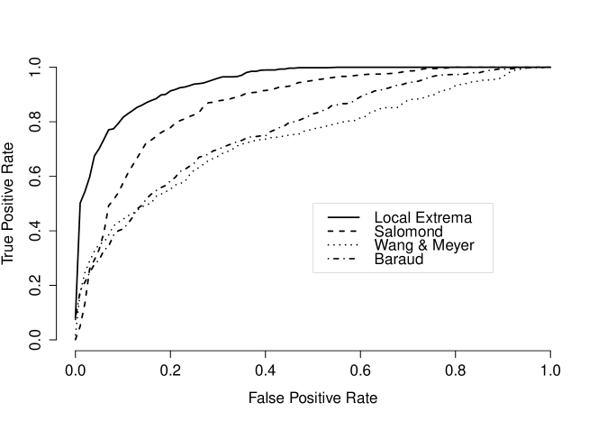
Figure 1 shows the receiver operating curve for hypothesis This figure shows that the local extrema approach is superior to the other three approaches across all false positive rates. Further, the estimated area under the receiver operating curve is which is excellent and better than the approach of Salomond at , Baraud at and Wang and Meyer at When looking at the impact of sample size on the tests, the power of the local extrema approach increases as the sample size increases, does so at a rate greater than competitors, and is similarly superior for hypothesis data not shown.
For hypothesis there is not an equivalent methodology in the literature, but performance of our approach is excellent. The area under the receiver operator curve is For the Bayes factor cut point of , table 2 gives results across all simulation conditions. Our test achieves high power for function even though this function is only slightly different than . Function is the same as , and this simulation gives evidence that the departure from monotonicity, which is concluded with high power hypothesis , may be due to the pronounced ‘U’ shape in the data, and not necessarily due to the fact that there are two extrema. As evident by the observed power, this feature requires more data to conclude .
| Function | n | |||
|---|---|---|---|---|
| 100 | 200 | 300 | 400 | |
| 78 | 90 | 98 | 96 | |
| 14 | 32 | 22 | 46 | |
| 76 | 88 | 98 | 100 | |
5 Applications
5.1 Estimating Muscle Force
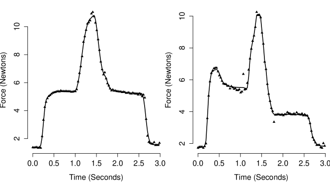
When studying the ability of a muscle to adapt to exercise protocols, muscle force tracings are often used. One approach involves first activating the muscle and then after a short period of time moving the joint through the range of motion (Baker et al.,, 2008). It is expected that the muscle force quickly obtains a maximum force with the observed force decreasing until joint movement; however, the observed force may plateau and not decrease before movement. When the joint is moved, there is an expected increase in the force output until the joint reaches a specific angle, after which, the observed force decreases until the joint reaches its original position. When the joint returns to its original position, the muscle remains activated and the force output is non-increasing until deactivation. Estimation of this muscle force curve may allow better understanding of adaptation or maladaptation following exercise, but it is important to include known biophysical constraints in curve estimation.
We model two force tracings ( per tracing) using a local extrema spline having at most local extrema. Consistent with prior knowledge of a very high signal to noise ratio, we place a prior on We also applied frequentist smoothing splines, Gaussian processes, and Bayesian P-splines. Competing methods are close to interpolating the data points, leaving unwanted artifactual bumps in the function estimate. However, as seen in Fig. 2, the local extrema spline obtains an estimate restricted to the known shape and robust to minor local fluctuations. Further, when the force tracing exhibits a single maxima, as in the left plot, the local extrema spline can readily distinguish between this shape, and a shape which has two maximum, as in the right plot, with no change in the model.
5.2 Seasonal Influenza and Pneumonia Death Rate
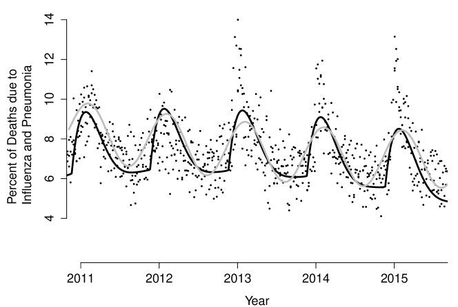
In temperate climates, the prevalence of influenza peaks in the winter months while dropping in the warmer months. Estimating this seasonal effect as well as departures from this effect, may be of interest when estimating the magnitude of an influenza epidemic. Here, we expect a peak in the winter months followed by a trough in the summer months. Parametric models for this pattern may not be adequate to model the observed phenomena, and smoothing approaches do not guarantee this pattern. We use local extrema splines, setting , to estimate this trend for Virginia, North Carolina and South Carolina for data collected by the Centers for Disease Control and Prevention National Center for Health Statistics Mortality surveillance branch.
Figure 3 plots the estimated mortality rates. These rates are estimated using an additive model defined by a quadratic trend representing a decrease in mortality over time, a seasonal component defined using local extrema spline, and a P-spline that represents departures from the overall trend. In this figure, the black curve represents the seasonally adjusted trend using the local extrema spline. This seasonal component is different than the trend published by the Centers for Disease Control, gray line (Viboud et al.,, 2010). The main difference between the two is the asymmetry in the local extrema approach during the winter months, which can not not be captured by a single sinusoidal function.
Acknowledgement
This research was partially supported by a grant from the National Institute of Environmental Health Sciences of the United States National Institutes of Health. The authors would like to thank Brent Baker for sharing the isometric muscle force data.
Appendix 1
Proofs of results
of Proposition 1.
It is well known that is continuous for and for all . Further, is a polynomial; therefore, is continuous with anti-derivative
If for all then for all and can only change sign when Thus, there are at most local extrema interior to with . ∎
of Theorem 1.
Consider where has exactly change-points. Functions with less than change points can be modeled by removing the required change point parameters from and continuing with the proof below.
Let be a taut B-spline approximation of of order defined on the knot set having exactly extrema such that
Here is defined on where As and are continuous and differentiable, we define such that and The measurable set of taut spline functions can be shown to exist (De Boor,, 2001) and we define a map where a subset of all possible local extrema spline functions with change points. Consider
| (7) |
and let For the exactly extrema in defined by the taut spline, set Additionally, if with odd, then set otherwise set In the case where with odd, then set otherwise set
Rewriting the RHS of (7) in a form based upon the derivative we have
where the derivative of is based upon the derivative formula for B-Splines (De Boor,, 2001) and
Because of the taut spline construction of we know that for all such that one has for all Here is the signum function. On each of these intervals let
As , we have further, one has
for all intervals such that
For the at most coefficients defined on splines that are nonzero in the intervals set these coefficients to zero. As there are a finite number of intervals whose error is non-zero and is bounded, the maximum error is at most for any and
Consequently, for any , consider taut B-spline constructions on knot sets such that that also have Then one has
∎
of Lemma 1.
The function in Theorem 1 is measurable. Given is measurable on some abstract measure space one has for any and some Given that the prior puts probability over knot sets having knot spacings that are arbitrarily close, that is as in Theorem 1, we conclude that for all . ∎
of Theorem 2.
We verify the conditions given in A1 and A2 of Theorem 1 of Choi and Schervish, (2007). Given that there is positive prior probability (Lemma 1) within all neighborhoods of one can use Choi and Schervish, (2007), section 4, to show the conditions of A1 of Theorem 1 are met. To verify A2 we have that and are subsets of all continuous differentiable functions on which were considered in Choi and Schervish, (2007); consequently, we appeal to Theorem and of Choi and Schervish, (2007) to construct suitable tests for both random and fixed designs using and We need only verify (iii) in part A2.
As in Choi and Schervish, (2007), assume that with We show that and for some Define as the design matrix given model and a particular configuration. Let and be the number of spline coefficients in model then
and by the Chernoff bounds
Now let be the probability of a branching process where is constant for all children, then there exists a such that for all such that Partition the sum into the finite sum where and the infinite sum As the finite sum is finite for all one has
where the last inequality exists as is bounded above zero, which implies one can choose some such that This implies that
A derivation similar to the above can be used to show the same holds for One can find a and substitute for and for in the above derivation∎. ∎
References
- Baker et al., (2008) Baker, B. A., Hollander, M. S., Mercer, R. R., Kashon, M. L., and Cutlip, R. G. (2008). Adaptive stretch-shortening contractions: diminished regenerative capacity with aging. Applied Physiology, Nutrition, and Metabolism, 33(6):1181–1191.
- Baraud et al., (2005) Baraud, Y., Huet, S., and Laurent, B. (2005). Testing convex hypotheses on the mean of a Gaussian vector. application to testing qualitative hypotheses on a regression function. Annals of statistics, pages 214–257.
- Biller, (2000) Biller, C. (2000). Adaptive Bayesian regression splines in semiparametric generalized linear models. Journal of Computational and Graphical Statistics, 9(1):122–140.
- Bornkamp and Ickstadt, (2009) Bornkamp, B. and Ickstadt, K. (2009). Bayesian nonparametric estimation of continuous monotone functions with applications to dose–response analysis. Biometrics, 65(1):198–205.
- Choi and Schervish, (2007) Choi, T. and Schervish, M. J. (2007). On posterior consistency in nonparametric regression problems. Journal of Multivariate Analysis, 98(10):1969–1987.
- De Boor, (2001) De Boor, C. (2001). A practical guide to splines, volume 27. Springer Verlag.
- DiMatteo et al., (2001) DiMatteo, I., Genovese, C. R., and Kass, R. E. (2001). Bayesian curve-fitting with free-knot splines. Biometrika, 88(4):1055–1071.
- Feller, (1974) Feller, W. (1974). Introduction to Probability Theory and Its Applications, Vol. I POD. John Wiley and Sons, New York.
- Genz, (1992) Genz, A. (1992). Numerical computation of multivariate normal probabilities. Journal of computational and graphical statistics, 1(2):141–149.
- Genz and Kwong, (2000) Genz, A. and Kwong, K.-S. (2000). Numerical evaluation of singular multivariate normal distributions. Journal of Statistical Computation and Simulation, 68(1):1–21.
- Geyer, (1991) Geyer, C. J. (1991). Markov chain Monte Carlo maximum likelihood. In Keramidas, E. M., editor, Computing Science and Statistics: Proceedings of the 23rd Symposium on the Interface. Interface Foundation of North America, Red Hook, NY.
- Geyer, (2011) Geyer, C. J. (2011). Importance sampling, simulated tempering and umbrella sampling. In Brooks, S., Gelman, A., Jones, G., and Meng, X., editors, Handbook of Markov Chain Monte Carlo, pages 295–311. Chapman & Hall/CRC, Boca Raton, FL.
- Godsill, (2001) Godsill, S. J. (2001). On the relationship between Markov chain Monte Carlo methods for model uncertainty. Journal of Computational and Graphical Statistics, 10(2):230–248.
- Green, (1995) Green, P. J. (1995). Reversible jump Markov chain Monte Carlo computation and Bayesian model determination. Biometrika, 82(4):711–732.
- Green and Silverman, (1993) Green, P. J. and Silverman, B. W. (1993). Nonparametric regression and generalized linear models: a roughness penalty approach. CRC Press.
- Hans and Dunson, (2005) Hans, C. and Dunson, D. (2005). Bayesian inferences on umbrella orderings. Biometrics, 61(4):1018–1026.
- Holmes and Mallick, (2003) Holmes, C. and Mallick, B. (2003). Generalized nonlinear modeling with multivariate free-knot regression splines. Journal of the American Statistical Association, 98(462):352–368.
- Lang and Brezger, (2004) Lang, S. and Brezger, A. (2004). Bayesian P-splines. Journal of Computational and Graphical Statistics, 13(1):183–212.
- Lavine and Mockus, (1995) Lavine, M. and Mockus, A. (1995). A nonparametric Bayes method for isotonic regression. Journal of Statistical Planning and Inference, 46(2):235–248.
- Meyer, (2008) Meyer, M. (2008). Inference using shape-restricted regression splines. The Annals of Applied Statistics, pages 1013–1033.
- Meyer et al., (2011) Meyer, M. C., Hackstadt, A. J., and Hoeting, J. A. (2011). Bayesian estimation and inference for generalised partial linear models using shape-restricted splines. Journal of Nonparametric Statistics, 23(4):867–884.
- Neelon and Dunson, (2004) Neelon, B. and Dunson, D. (2004). Bayesian isotonic regression and trend analysis. Biometrics, 60(2):398–406.
- Ramgopal et al., (1993) Ramgopal, P., Laud, P., and Smith, A. (1993). Nonparametric Bayesian bioassay with prior constraints on the shape of the potency curve. Biometrika, 80(3):489–498.
- Ramsay, (1988) Ramsay, J. (1988). Monotone regression splines in action. Statistical Science, pages 425–441.
- Salomond, (2014) Salomond, J.-B. (2014). Adaptive Bayes test for monotonicity. In The Contribution of Young Researchers to Bayesian Statistics, pages 29–33. Springer.
- Scott et al., (2015) Scott, J. G., Shively, T. S., and Walker, S. G. (2015). Nonparametric Bayesian testing for monotonicity. Biometrika, 102(3):617–630.
- Shi and Choi, (2011) Shi, J. Q. and Choi, T. (2011). Gaussian process regression analysis for functional data. CRC Press.
- Shively et al., (2009) Shively, T., Sager, T., and Walker, S. (2009). A Bayesian approach to non-parametric monotone function estimation. Journal of the Royal Statistical Society: Series B (Statistical Methodology), 71(1):159–175.
- Shively et al., (2011) Shively, T., Walker, S., and Damien, P. (2011). Nonparametric function estimation subject to monotonicity, convexity and other shape constraints. Journal of Econometrics, 161(2):166–181.
- Viboud et al., (2010) Viboud, C., Miller, M., Olson, D. R., Osterholm, M., and Simonsen, L. (2010). Preliminary estimates of mortality and years of life lost associated with the 2009 a/h1n1 pandemic in the us and comparison with past influenza seasons. PLoS currents, 2.
- Walker et al., (2004) Walker, S., Damien, P., and Lenk, P. (2004). On priors with a Kullback–Leibler property. Journal of the American Statistical Association, 99(466):404–408.
- Wang and Meyer, (2011) Wang, J. C. and Meyer, M. C. (2011). Testing the monotonicity or convexity of a function using regression splines. Canadian Journal of Statistics, 39(1):89–107.