Information Structures of Maximizing Distributions of Feedback Capacity for General Channels with Memory & Applications

Abstract

For any class of channel conditional distributions, with finite memory dependence on channel input RVs $A^{n}\stackrel{{\scriptstyle\triangle}}{{=}}\{A_{i}:i=0,\ldots,n\}$ or channel output RVs $B^{n}\stackrel{{\scriptstyle\triangle}}{{=}}\{B_{i}:i=0,\ldots,n\}$ or both, we characterize the sets of channel input distributions, which maximize directed information defined by

$$I(A^{n}\rightarrow B^{n})\stackrel{{\scriptstyle\triangle}}{{=}}\sum_{i=0}^{n}I(A^{i};B_{i}|B^{i-1})$$

and we derive the corresponding expressions, called “characterizations of Finite Transmission Feedback Information (FTFI) capacity”. The main theorems state that optimal channel input distributions occur in subsets ${\cal P}_{[0,n]}^{CI}\subseteq{\cal P}_{[0,n]}\stackrel{{\scriptstyle\triangle}}{{=}}\big{\{}{\bf P}_{A_{i}|A^{i-1},B^{i-1}}:i=0,\ldots,n\big{\}}$, which satisfy conditional independence on past information. We derive similar characterizations, when general transmission cost constraints are imposed. Moreover, we also show that the structural properties apply to general nonlinear and linear autoregressive channel models defined by discrete-time recursions on general alphabet spaces, and driven by arbitrary distributed noise processes.

We derive these structural properties by invoking stochastic optimal control theory and variational equalities of directed information, to identify tight upper bounds on $I(A^{n}\rightarrow B^{n})$, which are achievable over subsets of conditional distributions ${\cal P}_{[0,n]}^{CI}\subseteq{\cal P}_{[0,n]}$, which satisfy conditional independence and they are specified by the dependence of channel distributions and transmission cost functions on inputs and output symbols.

We apply the characterizations to recursive Multiple Input Multiple Output Gaussian Linear Channel Models with limited memory on channel input and output sequences, and we show a separation principle between the computation of the elements of the optimal strategies.

The structural properties of optimal channel input distributions, generalize the structural properties of Memoryless Channels with feedback, expressed in terms of conditional independence, to any channel distribution with memory, and settle various long standing open problems in information theory.

I Introduction

Shannon’s mathematical model of a communication channel with feedback is defined by

$$\Big{(}\big{\{}{\mathbb{A}}_{i}:i=-\infty,\ldots,n\big{\}},\big{\{}{\mathbb{B}}_{i}:i=-\infty,\ldots,n\big{\}},\big{\{}{\bf P}_{A_{i}|A^{i-1},B^{i-1}}:i=0,\ldots,n\big{\}},\big{\{}{\bf P}_{B_{i}|B^{i-1},A^{i}}:i=0,\ldots,n\big{\}}\Big{)}$$

where $a^{n}\stackrel{{\scriptstyle\triangle}}{{=}}\{\ldots,a_{-1},a_{0},a_{1},\ldots,a_{n}\}\in\times_{i=-\infty}^{n}{\mathbb{A}}_{i}$ are the channel input symbols, $b^{n}\stackrel{{\scriptstyle\triangle}}{{=}}\{\ldots,b_{-1},b_{0},b_{1},\ldots,b_{n}\}\in\times_{i=-\infty}^{n}{\mathbb{B}}_{i}$ are the channel output symbols, ${\cal P}_{[0,n]}\stackrel{{\scriptstyle\triangle}}{{=}}\big{\{}{\bf P}_{A_{i}|A^{i-1},B^{i-1}}:i=0,1,\ldots,n\big{\}}$ is the sequence of channel input conditional distributions with feedback, ${\cal C}_{[0,n]}\stackrel{{\scriptstyle\triangle}}{{=}}\big{\{}{\bf P}_{B_{i}|B^{i-1},A^{i}}:i=0,1,\ldots,n\big{\}}$ is the sequence of channel conditional distributions, and the initial distribution ${\bf P}_{A^{-1},B^{-1}}\equiv\nu(da^{-1},db^{-1})$ is fixed.
Shannon’s operational definion for reliable communication of information over the channel is described via a sequence of feedback codes $\{(n,{M}_{n},\epsilon_{n}):n=0,1,\dots\}$, which consist of the following elements.
(a) A set of uniformly distributed messages ${\cal M}_{n}\stackrel{{\scriptstyle\triangle}}{{=}}\{1,\ldots,M_{n}\}$ and a set of encoding strategies, mapping messages into channel inputs of block length $(n+1)$, defined by

$${\cal E}_{[0,n]}^{FB}(\kappa)\triangleq \Big{\{}g_{i}:{\cal M}_{n}\times{\mathbb{A}}^{i-1}\times{\mathbb{B}}^{i-1}\longmapsto{\mathbb{A}}_{i},\hskip 7.22743pta_{0}=g_{0}(w),a_{1}=g_{1}(w,a_{0},b_{0}),\ldots,a_{n}=g_{n}(w,a^{n-1},b^{n-1}),$$

$$\hskip 7.22743ptw\in{\cal M}_{n}:\hskip 7.22743pt\frac{1}{n+1}{\bf E}^{g}\Big{(}c_{0,n}(A^{n},B^{n-1})\Big{)}\leq\kappa\Big{\}},\hskip 7.22743ptn=0,1,\ldots.$$ (I.1)

The codeword for any $w\in{\cal M}_{n}$ is $u_{w}\in{\mathbb{A}}^{n}$, $u_{w}=(g_{0}(w),g_{1}(w,a_{0},b_{0}),\dots,g_{n}(w,a^{n-1},b^{n-1}))$, and ${\cal C}_{n}=(u_{1},u_{2},\dots,u_{{M}_{n}})$ is the code for the message set ${\cal M}_{n}$, and $\{A^{-1},B^{-1}\}=\{\emptyset\}$. In general, the code may depend on the initial data, depending on the convention, i.e., $(A^{-1},B^{-1})=(a^{-1},b^{-1})$, which are known to the encoder and decoder (unless specified otherwise).
(b) Decoder measurable mappings $d_{0,n}:{\mathbb{B}}^{n}\longmapsto{\cal M}_{n}$, such that the average probability of decoding error satisfies

$${\bf P}_{e}^{(n)}\triangleq\frac{1}{M_{n}}\sum_{w\in{\cal M}_{n}}{\bf P}^{g}\Big{\{}d_{0,n}(B^{n})\neq w|W=w\Big{\}}\equiv{\bf P}^{g}\Big{\{}d_{0,n}(B^{n})\neq W\Big{\}}\leq\epsilon_{n}$$

and the decoder may also assume knowledge of the initial data.
The coding rate or transmission rate over the channel is defined by $r_{n}\triangleq\frac{1}{n+1}\log M_{n}$. A rate $R$ is said to be an achievable rate, if there exists a code sequence satisfying $\lim_{n\longrightarrow\infty}{\epsilon}_{n}=0$ and $\liminf_{n\longrightarrow\infty}\frac{1}{n+1}\log{{M}_{n}}\geq R$.
The operational definition of feedback capacity of the channel is the supremum of all achievable rates, i.e., $C\triangleq\sup\{R:R\>\>\mbox{is achievable}\}$.

Given a source process $\big{\{}X_{i}:i=0,1,\ldots,\big{\}}$ with finite entropy rate, which is mapped into messages to be encoded and transmitted over the channel, and satisfies conditional independence [2]

$${\bf P}_{B_{i}|B^{i-1},A^{i},X^{k}}={\bf P}_{B_{i}|B^{i-1},A^{i}}\hskip 7.22743pt\forall k\in\{0,1,\ldots,n\},\hskip 7.22743pti=0,\ldots,n$$ (I.2)

under appropriate conditions, it is shown in [3, 4, 5], using tools from [6, 7, 8, 9, 10, 11, 12, 13], that the supremum of all achievable rates is characterized by the information quantity $C_{A^{\infty}\rightarrow B^{\infty}}^{FB}$, defined by the extremum problem

$$C_{A^{\infty}\rightarrow B^{\infty}}^{FB}\stackrel{{\scriptstyle\triangle}}{{=}}\liminf_{n\longrightarrow\infty}\frac{1}{n+1}C_{A^{n}\rightarrow B^{n}}^{FB},\hskip 14.45377ptC_{A^{n}\rightarrow B^{n}}^{FB}\stackrel{{\scriptstyle\triangle}}{{=}}\sup_{{\cal P}_{[0,n]}}I(A^{n}\rightarrow B^{n})$$ (I.3)

where $I(A^{n}\rightarrow B^{n})$ is the directed information from $A^{n}$ to $B^{n}$, defined by [14, 2]

$$I(A^{n}\rightarrow B^{n})\stackrel{{\scriptstyle\triangle}}{{=}} \sum_{i=0}^{n}I(A^{i};B_{i}|B^{i-1})=\sum_{i=0}^{n}{\bf E}_{\nu}\Big{\{}\log\Big{(}\frac{d{\bf P}_{B_{i}|B^{i-1},A^{i}}(\cdot|B^{i-1},A^{i})}{d{\bf P}_{B_{i}|B^{i-1}}(\cdot|B^{i-1})}(B_{i})\Big{)}\Big{\}}$$ (I.4)

Here, ${\bf E}_{\nu}\{\cdot\}$ denotes expectation with respect to the joint distribution induced by the channel input conditional distribution from ${\cal P}_{[0,n]}$, the specific channel conditional distribution from ${\cal C}_{[0,n]}$, and the initial distribution $\nu(da^{-1},db^{-1})$.
A fundamental problem in such extremum problems of directed information, is to determine the information structures of optimal channel input conditional distributions ${\cal P}_{[0,n]}\stackrel{{\scriptstyle\triangle}}{{=}}\big{\{}{\bf P}_{A_{i}|A^{i-1},B^{i-1}}:i=0,1,\ldots,n\big{\}}$, for any class of channel distributions, which maximize $I(A^{n}\rightarrow B^{n})$, equivalently, to characterize the subsets of ${\cal P}_{[0,n]}$ which satisfy conditional independence and maximize $I(A^{n}\rightarrow B^{n})$.

Our interest in the structural properties of optimization problem $C_{A^{n}\rightarrow B^{n}}^{FB}$ is the following. From the converse coding theorem [2, 15, 5], in view of (I.2), if the supremum over channel input distributions in $C_{A^{n}\rightarrow B^{n}}^{FB}$ exists, and its per unit time limit exists and it is finite, then $C_{A^{\infty}\rightarrow B^{\infty}}^{FB}$ is a non-trivial upper bound on the supremum of all achievable rates of feedback codes-the feedback capacity, while under stationary ergodicity or Dobrushin’s directed information stability [6, 7, 11, 4, 5], then $C_{A^{\infty}\rightarrow B^{\infty}}^{FB}$ is indeed the feedback capacity.
When transmission cost constraints are imposed of the form (or variants of them)

$${\cal P}_{[0,n]}(\kappa)\stackrel{{\scriptstyle\triangle}}{{=}}\Big{\{}{\bf P}_{A_{i}|A^{i-1},B^{i-1}},i=0,\ldots,n:\frac{1}{n+1}{\bf E}_{\nu}\Big{(}\sum_{i=0}^{n}\gamma_{i}(T^{i}A^{n},T^{i}B^{n})\Big{)}\leq\kappa\Big{\}},\hskip 7.22743pt\kappa\in[0,\infty)$$ (I.5)

the optimization problem (I.3) is replaced by

$$C_{A^{\infty}\rightarrow B^{\infty}}^{FB}(\kappa)\stackrel{{\scriptstyle\triangle}}{{=}}\liminf_{n\longrightarrow\infty}\frac{1}{n+1}C_{A^{n}\rightarrow B^{n}}^{FB}(\kappa),\hskip 14.45377ptC_{A^{n}\rightarrow B^{n}}^{FB}(\kappa)\stackrel{{\scriptstyle\triangle}}{{=}}\sup_{{\cal P}_{[0,n]}(\kappa)}I(A^{n}\rightarrow B^{n})$$ (I.6)

where for each $i$, the dependence of transmission cost function $\big{\{}\gamma_{i}(\cdot,\cdot):i=0,\ldots,n\big{\}}$, on input and output symbols is specified by $T^{i}a^{n}\subseteq\{a_{0},a_{1},\ldots,a_{i}\},T^{i}b^{n}\subseteq\{b_{0},b_{1},\ldots,b_{i}\}$, and these are either fixed or nondecreasing with $i$, for $i=0,1,\ldots,n$.

Our main objective is the following. Given a specific channel distribution and transmission cost function, we wish to determine the subsets of optimal channel input distributions ${\cal P}_{[0,n]}^{CI}\subseteq{\cal P}_{[0,n]}$ and ${\cal P}_{[0,n]}^{CI}(\kappa)\subseteq{\cal P}_{[0,n]}(\kappa)$, which satisfy conditional independence and correspond to the maximizing subsets of the extremum problems $C_{A^{n}\rightarrow B^{n}}^{FB}$ and $C_{A^{n}\rightarrow B^{n}}^{FB}(\kappa)$, respectively. Then to determine the corresponding characterizations, called Finite Transmission Feedback Information (FTFI) Capacity and Feedback capacity (i.e., their per unit time limiting versions), as it is done for Discrete Memoryless Channels (DMCs).

I-A Literature Review

Shannon and subsequently Dobrushin [16] characterized the capacity of DMCs (and memoryless channels with continuous alphabets, subject to transmission cost $\int|a|^{2}{\bf P}_{A}(da)\leq\kappa$), with and without feedback, and obtained the well-known two-letter expression

$$C\stackrel{{\scriptstyle\triangle}}{{=}}\max_{{\bf P}_{A}}I(A;B).$$ (I.7)

For memoryless channels without feedback, this characterization is obtained from the upper bound

$$C_{A^{n};B^{n}}\stackrel{{\scriptstyle\triangle}}{{=}}\max_{{\bf P}_{A^{n}}}I(A^{n};B^{n})\leq\;\max_{{\bf P}_{A_{i}},i=0,\ldots,n}\sum_{i=0}^{n}I(A_{i};B_{i})\leq(n+1)C.$$ (I.8)

since this bound is achievable, when the channel input distribution satisfies conditional independence ${\bf P}_{A_{i}|A^{i-1}}(da_{i}|a^{i-1})={\bf P}_{A_{i}}(da_{i}),i=0,1,\ldots,n$, and $\{A_{i}:i=0,1,\ldots,\}$ is identically distributed, which then implies the joint process $\{(A_{i},B_{i}):i=0,1,\ldots,\}$ is independent and identically distributed.
For memoryless channels with feedback, (I.7) is often obtained by first applying the converse to the coding theorem, to show that feedback does not increase capacity [1], which then implies

$${\bf P}_{A_{i}|A^{i-1},B^{i-1}}(da_{i}|a^{i-1},b^{i-1})={\bf P}_{A_{i}}(da_{i}),\hskip 7.22743pti=0,1,\ldots,n$$ (I.9)

and $C$ is obtained if $\{A_{i}:i=0,1,\ldots,\}$ is identically distributed. That is, since feedback does not increase capacity, then mutual information and directed information are identical, in view of (I.9). However, as pointed out elegantly by Massey [2], for channels with feedback it will be a mistake to use the same arguments as in (I.8). The conditional independence conditions imply that the Information Structure of the maximizing channel input distributions is the Null Set.
In Section III, we develop a methodology for directed information, which in principle, repeats the above steps, to show that for many classes of channel distribution with memory subject to transmission cost constraints, the optimal channel input distributions occur in subsets, characterized by conditional independence. However, each of the steps is more involved due to the memory of the channels, and hence new tools are introduced to established these achievable upper bounds.

Cover and Pombra [1] (see also [17, 11]) characterized the feedback capacity of non-stationary non-ergodic Additive Gaussian Noise (AGN) channels with memory, defined by

$$B_{i}=A_{i}+V_{i},\hskip 14.45377pti=0,1,\ldots,n,\hskip 14.45377pt\frac{1}{n+1}\sum_{i=0}^{n+1}{\bf E}\Big{\{}|A_{i}|^{2}\Big{\}}\leq\kappa,\hskip 7.22743pt\kappa\in[0,\infty)$$ (I.10)

where $\{V_{i}:i=0,1,\ldots,n\}$ is a real-valued jointly non-stationary Gaussian process $N(\mu_{V^{n}},K_{V^{n}})$, under the assumption that “$A^{n}$ is causally related to $V^{n}$” defined by

$${\bf P}_{A^{n},V^{n}}(da^{n},dv^{n})=\Big{(}\otimes_{i=0}^{n}{\bf P}_{A_{i}|A^{i-1},V^{i-1}}(da_{i}|a^{i-1},v^{i-1})\Big{)}\otimes{\bf P}_{V^{n}}(dv^{n}).$$ (I.11)

In [1], the authors characterized feedback capacity, via the maximization of mutual information between uniformly distributed messages and the channel output process, denoted by $I(W,B^{n})$, and obtained the following characterization .

$$C_{W;B^{n}}^{FB,CP}(\kappa)\stackrel{{\scriptstyle\triangle}}{{=}} \max_{\Big{\{}\frac{1}{n+1}\sum_{i=0}^{n}{\bf E}|A_{i}|^{2}\leq\>\kappa\Big{\}}}I(W,B^{n})=\max_{\Big{\{}\frac{1}{n+1}\sum_{i=0}^{n}{\bf E}|A_{i}|^{2}\leq\>\kappa:\hskip 7.22743ptA_{i}=\sum_{j=0}^{i-1}\overline{\gamma}_{i,j}V_{j}+\overline{Z}_{i}:\hskip 7.22743pti=0,1,\ldots,n\Big{\}}}H(B^{n})-H(V^{n})$$ (I.12)

$$= \sup_{\big{(}\overline{\Gamma}^{n},K_{\overline{Z}^{n}}\big{)}:\frac{1}{n+1}Tr\big{(}\overline{\Gamma}^{n}K_{{V}^{n}}\overline{\Gamma}^{T}+K_{\overline{Z}^{n}}\big{)}\leq\kappa}\frac{1}{2}\log\frac{\Big{|}\big{(}\overline{\Gamma}^{n}+I\big{)}K_{V^{n}}(\overline{\Gamma}^{n}+I)^{T}+K_{\overline{Z}^{n}}\Big{|}}{\Big{|}K_{V^{n}}\Big{|}}$$ (I.13)

where $\overline{Z}^{n}\stackrel{{\scriptstyle\triangle}}{{=}}\{\overline{Z}_{i}:i=0,1,\ldots,n\}$ is a Gaussian process $N(0,K_{{\overline{Z}}^{n}})$, orthogonal to $V^{n}\stackrel{{\scriptstyle\triangle}}{{=}}\{V_{i}:i=0,\ldots,n\}$, and $\{\overline{\gamma}_{i,j}:i,j=0,\ldots,n\}$ are deterministic functions, which constitute the entries of the lower diagonal matrix $\overline{\Gamma}^{n}$. The feedback capacity is shown to be $C_{W;B^{\infty}}^{FB,CP}(\kappa)\stackrel{{\scriptstyle\triangle}}{{=}}\lim_{n\longrightarrow\infty}\frac{1}{n+1}C_{W;B^{n}}^{FB,CP}(\kappa)$. Based on the characterization derived in [1], several investigations of versions of the Cover and Pombra [1] AGN channel are found in the literature, such as, [11, 18, 19]. Specifically, in [19], the stationary ergodic version of Cover and Pombra [1] AGN channel, is revisited by utilizing characterization (I.13) to derive expressions for feedback capacity, $C_{W;B^{\infty}}^{FB,CP}(\kappa)$, using frequency domain methods, when the noise power spectral density corresponds to a stationary Gaussian autoregressive moving-average model with finite memory. For finite alphabet channels with memory and feedback, expressions of feedback capacity are derived for certain channels with symmetry, in [20, 21, 22, 23, 24], while in [25] it is illustrated that if the input to the channel and the channel state are related by a one-to-one mapping, and the channel distribution is $\big{\{}{\bf P}_{B_{i}|A_{i},A_{i-1}}:i=0,\ldots,n\big{\}}$, then dynamic programming can be used, in such optimization problems. In [4], the general concepts of dynamic programming are related to the computation of feedback capacity for Markov Channels (Definition 6.1 in [4]). In [26] the unit memory channel output (UMCO) channel $\big{\{}{\bf P}_{B_{i}|B_{i-1},A_{i}}:i=0,\ldots,n\}$, is analyzed under the assumption that the optimal channel input distribution is $\big{\{}{\bf P}_{A_{i}|B_{i-1}}:i=0,\ldots,n\}$.

I-B Channel Models and Transmission Cost Functions: Motivation and Objectives

In general, it is almost impossible, to determine the information structures of optimal channel input distributions directly from $C_{A^{\infty}\rightarrow B^{\infty}}^{FB}$ and $C_{A^{\infty}\rightarrow B^{\infty}}^{FB}(\kappa)$. Indeed, in the related theory of infinite horizon Markov Decision (MD), the fundamental question, whether optimizing the expected value of a fixed pay-off functional over all non-Markov strategies occurs in the subclass of Markov strategies, is addressed from its finite horizon version. Then by using the Markovian property of strategies, the infinite horizon or per unit time limit (i.e., asymptotic limit) over Markov strategies is analyzed [27].
However, classical stochastic optimal control or MD theory, is not directly applicable to extremum problems of directed information, such as, (I.4), because the pay-off functional is the directed information density,

$$\iota_{A^{n}\rightarrow B^{n}}(A^{n},B^{n})\stackrel{{\scriptstyle\triangle}}{{=}}\sum_{i=0}^{n}\frac{d{\bf P}_{B_{i}|B^{i-1},A^{i}}(\cdot|B^{i-1},A^{i})}{d{\bf P}_{B_{i}|B^{i-1}}(\cdot|B^{i-1})}(B_{i})$$ (I.14)

and this pay-off depends nonlinearly on the channel input conditional distribution $\{{\bf P}_{A_{i}|A^{i-1},B^{i-1}}:i=0,\ldots,n\}$ via the channel output conditional distribution $\{{\bf P}_{B_{i}|B^{i-1}}:i=0,\ldots,n\}$. This means, for general extremum problems of feedback capacity, the information structure of optimal channel input distribution needs to be identified, before any method can be applied to compute feedback capacity, such as, the identification of sufficient statistics and dynamic programming [27, 28].

In this paper, our main objective is to determine the information structures of optimal channel input distributions, by characterizing the subsets of channel input distributions ${\cal P}_{[0,n]}^{CI}\subseteq{\cal P}_{[0,n]}$ and ${\cal P}_{[0,n]}^{CI}(\kappa)\subseteq{\cal P}_{[0,n]}(\kappa)$, which satisfy conditional independence, and give tight upper bounds on directed information $I(A^{n}\rightarrow B^{n})$, which are achievable, called the “characterizations of Finite Transmission Feedback Information (FTFI) capacity”.
We derive characterizations of FTFI capacity for any class of time-varying channel distributions and transmission cost functions, of the following type.

Channel Distributions.

$$\mbox{\bf Class A.}\hskip 7.22743pt{\bf P}_{B_{i}|B^{i-1},A^{i}}(db_{i}|b^{i-1},a^{i})={\bf P}_{B_{i}|B^{i-1},A_{i-L}^{i}}(db_{i}|b^{i-1},a_{i-L}^{i}),\hskip 7.22743pti=0,\ldots,n,$$ (I.15)

$$\mbox{\bf Class B.}\hskip 7.22743pt{\bf P}_{B_{i}|B^{i-1},A^{i}}(db_{i}|b^{i-1},a^{i})={\bf P}_{B_{i}|B_{i-M}^{i-1},A_{i}}(db_{i}|b_{i-M}^{i-1},a^{i}),\hskip 7.22743pti=0,\ldots,n,$$ (I.16)

$$\mbox{\bf Class C.}\hskip 7.22743pt{\bf P}_{B_{i}|B^{i-1},A^{i}}(db_{i}|b^{i-1},a^{i})={\bf P}_{B_{i}|B_{i-M}^{i-1},A_{i-L}^{i}}(db_{i}|b_{i-M}^{i-1},a_{i-L}^{i}),\hskip 7.22743pti=0,\ldots,n.$$ (I.17)

Transmission Cost Functions.

$$\mbox{\bf Class A.}\hskip 7.22743pt\gamma_{i}(T^{i}a^{n},T^{i}b^{n})={\gamma}_{i}^{A.N}(a_{i-N}^{i},b^{i}),\hskip 14.45377pti=0,\ldots,n,$$ (I.18)

$$\mbox{\bf Class B.}\hskip 7.22743pt\gamma_{i}(T^{i}a^{n},T^{i}b^{n})={\gamma}_{i}^{B.K}(a^{i},b_{i-K}^{i}),\hskip 14.45377pti=0,\ldots,n,$$ (I.19)

$$\mbox{\bf Class C.}\hskip 7.22743pt\gamma_{i}(T^{i}a^{n},T^{i}b^{n})={\gamma}_{i}^{C.N,K}(a_{i-N}^{i},b_{i-K}^{i}),\hskip 14.45377pti=0,\ldots.n,$$ (I.20)

Here, $\{K,L,M,N\}$ are nonnegative finite integers and we use the following convention.

$$\mbox{If $M=0$ then}\hskip 7.22743pt{\bf P}_{B_{i}|B_{i-M}^{i-1},\overline{A}^{i}}(db_{i}|b_{i-M}^{i-1},\overline{a}^{i})|_{M=0}={\bf P}_{B_{i}|\overline{A}^{i}}(db_{i}|\overline{a}^{i}),\hskip 7.22743pt\mbox{for any}\hskip 7.22743pt\overline{A}^{i}\in\{A^{i},A_{i-L}^{i}\},\hskip 7.22743pti=0,1,\ldots,n.$$

For $M=L=0$, the channel is memoryless. By invoking function restriction, if necessary, the above transmission cost functions include, as degenerate cases, many others, such as, $\gamma_{i}(\cdot,T^{i}b^{n})={\gamma}_{i}(\cdot,b_{i-K}^{i-1}),i=0,\ldots,n$. In this paper we do not treat the case $L=N=0$, because these are investigated in [29]. However, we provide discussions on the fundamental differences of the information structures of optimal channel input distributions, when the channels and transmission cost functions depend on past channel inputs, compared to $L=N=0$.
Channel distributions of Class A, B or C, i.e., (I.15)-(I.17), are induced by various nonlinear channel models (NCM) driven by noise processes [30].

We also derive characterizations of FTFI capacity for any channel distribution induced by recursive Nonlinear Channel Models (NCM) driven by arbitrary distributed noise process $\{V_{i}:i=0,\ldots,n\}$ with memory and arbitrary alphabet spaces $\{{\mathbb{V}}_{i}:i=0,\ldots,n\}$, of the following type.

Nonlinear Channel Models with Correlated Noise.

$$B_{i}=h_{i}^{D}(\overline{B}^{i-1},\overline{A}^{i},V_{i})\hskip 14.45377pt\mbox{for any}\hskip 7.22743pt\overline{A}^{i}\in\{A^{i},A_{i-L}^{i}\},\hskip 7.22743pt\overline{B}^{i-1}\in\{B^{i-1},B_{i-M}^{i-1}\},\hskip 7.22743pti=0,\ldots,n,$$ (I.21)

$$\frac{1}{n+1}{\bf E}_{\nu}\Big{\{}\sum_{i=0}^{n}\gamma_{i}(T^{i}A^{n},T^{i}B^{n})\Big{\}}\leq\kappa,$$ (I.22)

$${\bf P}_{V_{i}|V^{i-1},A^{i}}(dv_{i}|v^{i-1},a^{i})={\bf P}_{V_{i}|\overline{V}^{i-1}}(dv_{i}|\overline{v}^{i-1}),\hskip 7.22743pt\overline{v}^{i-1}\in\big{\{}v_{i-T}^{i-1},v^{i-1}\big{\}},\hskip 7.22743pti=0,\ldots,n$$ (I.23)

where $\{h_{i}^{D}(\cdot,\cdot,\cdot):i=0,\ldots,n\}$ are nonlinear mappings and $B_{-M}^{-1}=b_{-M}^{-1},A_{-L}^{-1}=a_{-L}^{-1}$ are the initial data.
Specifically, we show that we can apply the main theorems of the characterizations of FTFI capacity for Class A, B, C channels and tranmsission cost functions, with slight modification, to derive the characterizations of FTFI capacity for NCMs with correlated noise.

The channel distributions of Class A, B, C and the NCMs include nonlinear and linear time-varying autoregressive models and linear channel models expressed in state space form [30]. Our main theorems generalize many existing results found in the literature, for example, non-stationary and non-ergodic Additive Gaussian Noise channels investigated by Cover and Pombra [1] and stationary deterministic channels [31], and finite alphabet channels with channel state information investigated in [26, 25, 20, 22, 21, 23, 24]. However, the derivations of characterizations of FTFI capacity and realizations of optimal channel input distributions by random processes are fundamentally different from any of the above references.

I-C Methodology & Main Results

The methodology we apply to derive the information structures of optimal channel input distributions and the corresponding characterizations of FTFI capacity, combines stochastic optimal control theory [32] and variational equalities of directed information [33]. This method is applied in [29] to derive characterizations of FTFI capacity for channel distributions of Class A and C, with $L=0$, with and without transmission cost functions of Class A or C, with $N=0$.
In this paper, we apply the method with some variations, to any combination of channel distributions and transmission cost functions of class A, B, C, and to NCMs with correlated noise, as follows.

Class A, B, C Channel Distributions and Transmission Cost Functions.
First, we identify the connection between stochastic optimal control theory and extremum problems $C_{A^{n}\rightarrow B^{n}}^{FB},C_{A^{n}\rightarrow B^{n}}^{FB}(\kappa)$ (see also Figure I.1), as follows.

(i)

The information measure $I(A^{n}\rightarrow B^{n})$ is the pay-off;

(ii)

the channel output process $\{B_{i}:i=0,1,\ldots,n\}$ is the controlled process;

(iii)

the channel input process $\{A_{i}:i=0,1,\ldots,n\}$ is the control process;

(iv)

the channel output process $\{B_{i}:i=0,1,\ldots,n\}$ is controlled, by controlling the conditional probability distribution $\big{\{}{\bf P}_{B_{i}|B^{i-1}}:i=0,\ldots,n\big{\}}$, via the choice of the transition probability distribution $\big{\{}{\bf P}_{A_{i}|A^{i-1},B^{i-1}}:i=0,\ldots,n\big{\}}\in{\cal P}_{[0,n]}$ or ${\cal P}_{[0,n]}(\kappa)$ called the control object.

Second, we identify variational equalities of directed information, which can be used to determine achievable upper bounds on directed information over subsets of channel input conditional distributions, ${\cal P}_{[0,n]}^{CI}(\kappa)\subseteq{\cal P}_{[0,n]}(\kappa)$, characterized by conditional independence.

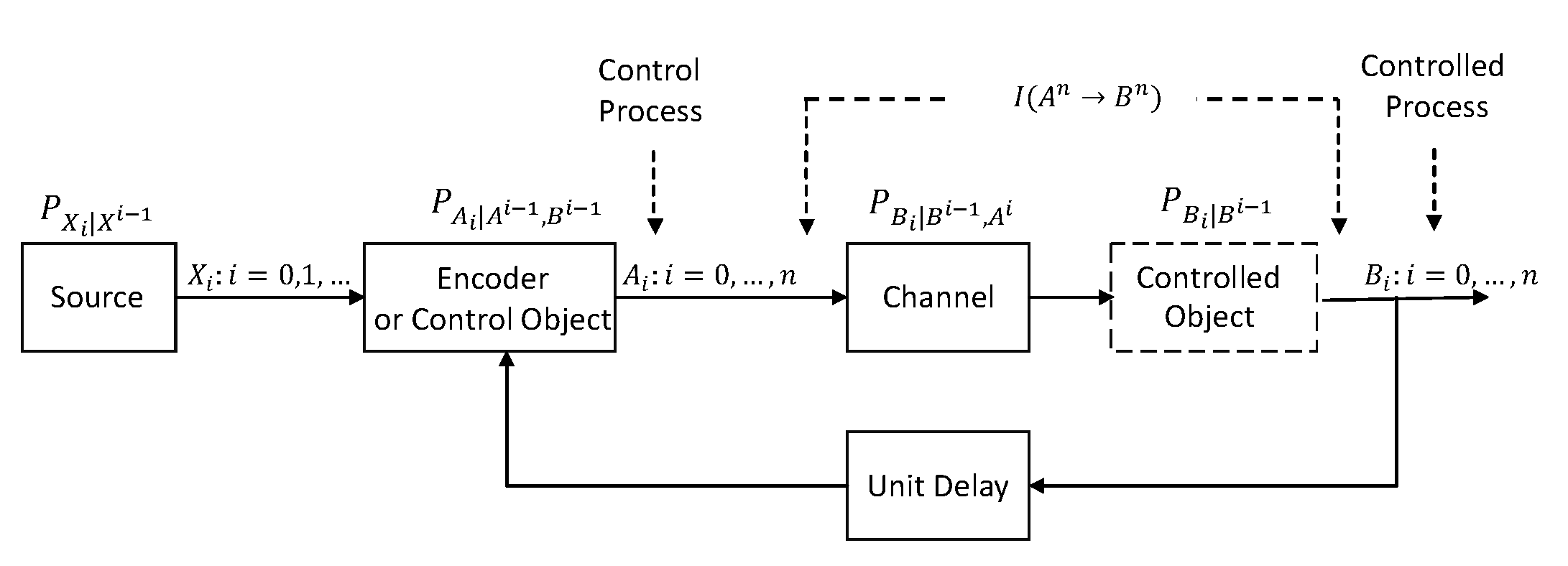
Figure I.1: Communication block diagram and its analogy to stochastic optimal control.

We show that for any combination of channel distributions and transmission cost functions of class A, B, or C, the maximization of $I(A^{n}\rightarrow B^{n})$ over ${\cal P}_{[0,n]}(\kappa)$, occurs in a subset ${\cal P}_{[0,n]}^{CI}(\kappa)$, which satisfy conditional independence, as follows.

$${\cal P}_{[0,n]}^{CI}(\kappa)\stackrel{{\scriptstyle\triangle}}{{=}}\Big{\{}{\bf P}_{A_{i}|A^{i-1},B^{i-1}}(da_{i}|a^{i-1},b^{i-1})={\pi}_{i}(da_{i}|{\cal I}_{i}^{\bf P})\equiv{\mathbb{P}}\big{\{}A_{i}\in da_{i}|{\cal I}_{i}^{\bf P}\big{\}}:i=0,\ldots,n\Big{\}}\bigcap{\cal P}_{[0,n]}(\kappa),$$ (I.24)

$${\cal I}_{i}^{\bf P}\subseteq\big{\{}a^{i-1},b^{i-1}\big{\}},\hskip 7.22743pti=0,\ldots,n,$$ (I.25)

$${\cal I}_{i}^{\bf P}\stackrel{{\scriptstyle\triangle}}{{=}}\>\mbox{Information Structure of optimal channel input distributions for $i=0,\ldots,n$}.$$ (I.26)

Further, we show that the information structure ${\cal I}_{i}^{{\bf P}},i=0,1,\ldots,n$, is specified by the memory of the channel conditional distribution, and the dependence of the transmission cost function on the channel input and output symbols. This procedure allows us to determine the dependence, of the joint distribution of $\{(A_{i},B_{i}):i=0,\ldots,n\}$, and the conditional distribution $\{{\bf P}_{B_{i}|B^{i-1}}:i=0,\ldots,n\}$ on the control object, $\big{\{}{\pi}_{i}(da_{i}|{\cal I}_{i}^{\bf P}):i=0,\ldots,\big{\}}$, and to determine the characterizations of FTFI capacity.

NCMs with Correlated Noise.
For any NCM defined by (I.21)-(I.23), with limited memory, i.e., $\big{\{}\overline{A}^{i},\overline{B}^{i-1},\overline{V}^{i}\big{\}}=\big{\{}A_{i-L}^{i},B_{i-M}^{i-1},V_{i-T}^{i}\big{\}},\gamma_{i}(\cdot,\cdot)=\gamma_{i}^{C.L,M}(\cdot,\cdot),i=0,\ldots,n$, and under the assumption that the functions mappings for fixed $(b_{i-M}^{i-1},a_{i-L}^{i})$ defined by

$$h_{i}^{D}(b_{i-M}^{i-1},a_{i-L}^{i},\cdot):{\mathbb{V}}_{i}\longmapsto h_{i}^{D}(b_{i-M}^{i-1},a_{i-L}^{i},v_{i}),\hskip 7.22743pti=0,\ldots,n$$ (I.27)

are invertible and measurable, with inverse $\overline{h}_{i}^{D}(b_{i},b_{i-M}^{i-1},a_{i-L}^{i}),i=0,\ldots,n$, we first apply the converse to the coding theorem to derive the tight upper bound

$$R\leq\liminf_{n\longrightarrow\infty}\frac{1}{n+1}{C}_{W;B^{n}}^{FB,D}(\kappa)$$ (I.28)

where

$${C}_{W;B^{n}}^{FB,D}(\kappa)\stackrel{{\scriptstyle\triangle}}{{=}}\sup_{{\cal P}_{[0,n]}^{D}(\kappa)}\sum_{i=0}^{n}I(A_{i-L}^{i},V_{i-T}^{i-1};B_{i}|B^{i-1}),$$ (I.29)

$${\cal P}_{[0,n]}^{D}(\kappa)\stackrel{{\scriptstyle\triangle}}{{=}}\Big{\{}{\bf P}_{A_{i}|A^{i-1},V^{i-1},B^{i-1}},i=0,\ldots,n:\frac{1}{n+1}{\bf E}_{\nu}\Big{(}\sum_{i=0}^{n}\gamma_{i}^{C.L,M}(A_{i-L}^{i},B_{i-M}^{i})\leq\kappa\Big{)}\Big{\}}.$$ (I.30)

That is, ${C}_{W;B^{n}}^{FB,D}(\kappa)$ is the analog of ${C}_{A^{n}\rightarrow B^{n}}^{FB}(\kappa)$. Then we show that the methodology described above for Class A, B, C channels and transmission costs, with slight variations, is directly applicable, and we derive characterizations of the FTFI capacity, by showing that the maximization in (I.29), occurs in subsets of ${\cal P}_{[0,n]}^{D}(\kappa)$, which satisfy conditional independence.

We emphasize that our objective and methodology descibed above, are fundamentally different from any derivations given in the literature, such as, Theorem 1 in [25], Theorem 1 in [18], Theorem 1 in [20], and further adopted in subsequent work in [21, 22]. Specifically, we show that the supremum of directed information over all channel input conditional distributions occurs in a smaller set, satisfying a conditional independence condition, which is analogous to (I.24). This is different from the derivations given in [25, 18, 20]. This point is further elaborated in Section III.

In Section II, we introduce the notation and the variational equalities of directed information.
In Section III, we derive the information structures of optimal channel input distributions for any combination of channel distributions and transmission cost functions of Class A, B or C.
In section IV, we consider the application example of general Multiple-Input Multiple-Output (MIMO) Gaussian channels with memory on past channel input and output symbols, and quadratic cost constraint, i.e., class C, with $L=M=1$. We show that the optimal channel input distribution corresponding to the characterization of the FTFI capacity exhibits a separation principle. We show this separation principle by using the orthogonal decomposition of realizations of optimal channel input distributions.
Via the separation principle, we derive an expression for the optimal channel input distribution, and we relate the characterization of FTFI capacity to the so-called Linear-Quadratic-Gaussian partially observable stochastic optimal control problem [27].
In Section V, we first derive a converse to the coding theorem for NCMs defined by (I.21)-(I.23) and (I.27) and then we derive analogous information structures of optimal channel input distributions and corresponding characterizations of FTFI capacity.
Throughout the paper we relate the characterizations of FTFI capacity of various channels and the realizations of optimal channel input distributions to existing results given in the literature.

II Extremum problems of Directed Information and Variational Equalities

In this section, we introduce the basic notation, the precise definition of extremum problem of FTFI capacity (I.3), the variational equalities of directed information [34], and some of their properties.

Throughout the paper we use the following notation.

$${\mathbb{R}}:\hskip 7.22743pt\mbox{set of real numbers};$$

$${\mathbb{Z}}:\hskip 7.22743pt\mbox{set of integer};$$

$${\mathbb{N}}_{0}:\hskip 7.22743pt\mbox{set of nonnegative integers}\hskip 7.22743pt\{0,1,2,\dots\};$$

$${\mathbb{R}}^{n}:\hskip 7.22743pt\mbox{set of $n$ tuples of real natural};$$

$${\mathbb{S}}_{+}^{p\times p}:\hskip 7.22743pt\mbox{set of symmetric positive semi-define}\ p\times p\hskip 7.22743pt\mbox{matrices}\ A\in{\mathbb{R}}^{p\times p};$$

$${\mathbb{S}}_{++}^{p\times p}:\hskip 7.22743pt\mbox{subset of positive definite matrices of the set}\hskip 7.22743pt{\mathbb{S}}_{+}^{p\times p};$$

$$\langle\cdot,\cdot\rangle:\hskip 7.22743pt\mbox{inner product of elements of vectors spaces;}$$

$$(\Omega,{\cal F},{\mathbb{P}}):\mbox{probability space, where ${\cal F}$ is the $\sigma-$algebra generated by subsets of $\Omega$};$$

$${\cal B}({\mathbb{W}}):\hskip 7.22743pt\mbox{Borel $\sigma-$algebra of a given topological space ${\mathbb{W}}$};$$

$${\cal M}({\mathbb{W}}):\hskip 7.22743pt\mbox{set of all probability measures on ${\cal B}({\mathbb{W}})$ of a Borel space ${\mathbb{W}}$};$$

$${\cal K}({\mathbb{V}}|{\mathbb{W}}):\hskip 7.22743pt\mbox{set of all stochastic kernels on $({\mathbb{V}},{\cal B}({\mathbb{V}}))$ given $({\mathbb{W}},{\cal B}({\mathbb{W}}))$ of Borel spaces ${\mathbb{W}},{\mathbb{V}}$};$$

All spaces (unless stated otherwise) are complete separable metric spaces also called Polish spaces, i.e., Borel spaces. This generalization is adopted to treat simultaneously discrete, finite alphabet, real-valued ${\mathbb{R}}^{k}$ or complex-valued ${\mathbb{C}}^{k}$ random processes for any positive integer $k$, and general ${\mathbb{R}}^{k}-$valued random processes with absolute summable $p$-moments, $p=1,2,\ldots$, (see [35]) etc.

Given two measurable spaces $({\mathbb{X}},{\cal B}({\mathbb{X}}))$, $({\mathbb{Y}},{\cal B}({\mathbb{Y}}))$ then ${\mathbb{X}}\times{\mathbb{Y}}\stackrel{{\scriptstyle\triangle}}{{=}}\{(x,y):x\in{\mathbb{X}},y\in{\mathbb{Y}}\}$ is the cartesian product of ${\mathbb{X}}$ and ${\mathbb{Y}}$, and for $A\in{\cal B}({\mathbb{X}})$ and $B\in{\cal B}({\mathbb{Y}})$ then $A\times B$ is called a measurable rectangle. The product measurable space of $({\mathbb{X}},{\cal B}({\mathbb{X}}))$ and $({\mathbb{Y}},{\cal B}({\mathbb{Y}}))$ is denoted by $({\mathbb{X}}\times{\mathbb{Y}},{\cal B}({\mathbb{X}})\otimes{\cal B}({\mathbb{Y}}))$, where ${\cal B}({\mathbb{X}})\otimes{\cal B}({\mathbb{Y}})$ is the product $\sigma-$algebra generated by $\{A\times B:A\in{\cal B}({\mathbb{X}}),B\in{\cal B}({\mathbb{Y}})\}$.
A Random Variable (RV) defined on a probability space $(\Omega,{\cal F},{\mathbb{P}})$ by the mapping $X:(\Omega,{\cal F})\longmapsto({\mathbb{X}},{\cal B}({\mathbb{X}}))$ induces a probability distribution ${\bf P}(\cdot)\equiv{\bf P}_{X}(\cdot)$ on $({\mathbb{X}},{\cal B}({\mathbb{X}}))$ as follows.

$${\bf P}(A)\equiv{\bf P}_{X}(A)\stackrel{{\scriptstyle\triangle}}{{=}}{\mathbb{P}}\big{\{}\omega\in\Omega:X(\omega)\in A\big{\}},\hskip 7.22743pt\forall A\in{\cal B}({\mathbb{X}}).$$ (II.31)

A RV is called discrete if there exists a countable set ${\cal S}_{X}\stackrel{{\scriptstyle\triangle}}{{=}}\{x_{i}:i\in{\mathbb{N}}_{0}\}$ such that $\sum_{x_{i}\in{\cal S}_{X}}{\mathbb{P}}\{\omega\in\Omega:X(\omega)=x_{i}\}=1$. The probability distribution ${\bf P}_{X}(\cdot)$ is then concentrated on points in ${\cal S}_{X}$, and it is defind by

$${\bf P}_{X}(A)\stackrel{{\scriptstyle\triangle}}{{=}}\sum_{x_{i}\in{\cal S}_{X}\bigcap A}{\mathbb{P}}\big{\{}\omega\in\Omega:X(\omega)=x_{i}\big{\}},\hskip 7.22743pt\forall A\in{\cal B}({\mathbb{X}}).$$ (II.32)

If the cardinality of ${\cal S}_{X}$ is finite then the RV is finite-vaued and it is called a finite alphabet RV.
Given another RV $Y:(\Omega,{\cal F})\longmapsto({\mathbb{Y}},{\cal B}({\mathbb{Y}}))$, ${\bf P}_{Y|X}(dy|X)(\omega)$ is called the conditional distribution of RV $Y$ given RV $X$. The conditional distribution of RV $Y$ given $X=x$ is denoted by ${\bf P}_{Y|X}(dy|X=x)\equiv{\bf P}_{Y|X}(dy|x)$. Such conditional distributions are equivalently described by stochastic kernels or transition functions ${\bf K}(\cdot|\cdot)$ on ${\cal B}({\mathbb{Y}})\times{\mathbb{X}}$, mapping ${\mathbb{X}}$ into ${\cal M}({\mathbb{Y}})$ (the space of probability measures on $({\mathbb{Y}},({\cal B}({\mathbb{Y}}))$, i.e., $x\in{\mathbb{X}}\longmapsto{\bf K}(\cdot|x)\in{\cal M}({\mathbb{Y}})$, such that for every $F\in{\cal B}({\mathbb{Y}})$, the function ${\bf K}(F|\cdot)$ is ${\cal B}({\mathbb{X}})$-measurable.
The family of such probability distributions on $({\mathbb{Y}},{\cal B}({\mathbb{Y}}))$ parametrized by $x\in{\mathbb{X}}$, is defined by ${\cal K}({\mathbb{Y}}|{\mathbb{X}})\stackrel{{\scriptstyle\triangle}}{{=}}\Big{\{}{\bf K}(\cdot|x)\in{\cal M}({\mathbb{Y}}):\hskip 7.22743ptx\in{\mathbb{X}}\Big{\}}$.

II-A FTFI Capacity and Variational Equalities

The communication block diagram is shown in Figure I.1. The channel input and channel output alphabets are sequences of Polish measurable spaces (complete separable metric spaces) $\{({\mathbb{A}}_{i},{\cal B}({\mathbb{A}}_{i})):i\in\mathbb{Z}\}$ and $\{({\mathbb{B}}_{i},{\cal B}({\mathbb{B}}_{i})):i\in\mathbb{Z}\}$, respectively, and their history spaces are the product spaces ${\mathbb{A}}^{\mathbb{Z}}\stackrel{{\scriptstyle\triangle}}{{=}}{{\times}_{i\in\mathbb{Z}}}{\mathbb{A}}_{i},$ ${\mathbb{B}}^{\mathbb{Z}}\stackrel{{\scriptstyle\triangle}}{{=}}{\times_{i\in\mathbb{Z}}}{\mathbb{B}}_{i}$. These spaces are endowed with their respective product topologies, and ${\cal B}({\Sigma}^{\mathbb{Z}})\stackrel{{\scriptstyle\triangle}}{{=}}\otimes_{i\in\mathbb{Z}}{\cal B}({\Sigma}_{i})$, denotes the $\sigma-$algebra on ${\Sigma}^{\mathbb{Z}}$, where ${\Sigma}_{i}\in\big{\{}{\mathbb{A}}_{i},{\mathbb{B}}_{i}\big{\}}$, ${\Sigma}^{\mathbb{Z}}\in\big{\{}{\mathbb{A}}^{\mathbb{Z}},{\mathbb{B}}^{\mathbb{Z}}\big{\}}$, generated by cylinder sets. Points in ${\Sigma}_{k}^{m}\stackrel{{\scriptstyle\triangle}}{{=}}\times_{j=k}^{m}{\Sigma}_{j}$ are denoted by $z_{k}^{m}\stackrel{{\scriptstyle\triangle}}{{=}}\{z_{k},z_{k+1},\ldots,z_{m}\}\in{\Sigma}_{k}^{m}$, $(k,m)\in{\mathbb{Z}}\times{\mathbb{Z}}$.

Next, we introduce the various distributions.

Channel Distributions with Memory. A sequence of stochastic kernels or distributions defined by

$${\cal C}_{[0,n]}\stackrel{{\scriptstyle\triangle}}{{=}}\Big{\{}Q_{i}(db_{i}|b^{i-1},a^{i})={\bf P}_{B_{i}|B^{i-1},A^{i}}\in{\cal K}({\mathbb{B}}_{i}|{\mathbb{B}}^{i-1}\times{\mathbb{A}}^{i}):i=0,1,\ldots,n\Big{\}}.$$ (II.33)

At each time instant $i$ the conditional distribution of the channel is affected causally by past channel output symbols $b^{i-1}\in{\mathbb{B}}^{i-1}$ and current and past channel input symbols $a^{i}\in{\mathbb{A}}^{i},i=0,1,\ldots,n$.

Channel Input Distributions with Feedback. A sequence of stochastic kernels defined by

$${\cal P}_{[0,n]}\stackrel{{\scriptstyle\triangle}}{{=}}\Big{\{}P_{i}(da_{i}|a^{i-1},b^{i-1})={\bf P}_{A_{i}|A^{i-1},B^{i-1}}\in{\cal K}({\mathbb{A}}_{i}|{\mathbb{A}}^{i-1}\times{\mathbb{B}}^{i-1}):i=0,1,\ldots,n\Big{\}}.$$ (II.34)

At each time instant $i$ the conditional channel input distribution with feedback is affected causally by past channel inputs and output symbols $\{a^{i-1},b^{i-1}\}\in{\mathbb{A}}^{i-1}\times{\mathbb{B}}^{i-1},i=0,1,\ldots,n$.

Admissible Histories. For each $i=-1,0,\ldots,n$, we introduce the space ${\mathbb{G}}^{i}$ of admissible histories of channel input and output symbols, as follows. Define

$${\mathbb{G}}^{i}\triangleq{\mathbb{A}}^{-1}\times{\mathbb{B}}^{-1}\times\mathbb{A}_{0}\times\mathbb{B}_{0}\times\ldots\times\mathbb{A}_{i-1}\times\mathbb{B}_{i-1}\times\mathbb{A}_{i}\times{\mathbb{B}}_{i},\;i=0,\ldots,n,\;{\mathbb{G}}^{-1}={\mathbb{A}}^{-1}\times{\mathbb{B}}^{-1}.$$ (II.35)

A typical element of ${\mathbb{G}}^{i}$ is a sequence of the form $(a^{-1},b^{-1},a_{0},b_{0},\ldots,a_{i},b_{i})$. We equip the space ${\mathbb{G}}^{i}$ with the natural $\sigma$-algebra ${\cal B}({\mathbb{G}}^{i})$, for $i=-1,0,\ldots,n$. Hence, for each $i$, the information structure of the channel input distribution is

$${\cal I}_{i}^{P}\stackrel{{\scriptstyle\triangle}}{{=}}\Big{\{}A^{-1},B^{-1},A_{0},B_{0},\ldots,A_{i-1},B_{i-1}\Big{\}},\;i=0,1,\ldots,n,\hskip 14.45377pt{\cal I}_{0}^{P}\stackrel{{\scriptstyle\triangle}}{{=}}\big{\{}A^{-1},B^{-1}\big{\}}.$$ (II.36)

This implies at time $i=0$, the initial distribution is $P_{0}(da_{0}|a^{-1},b^{-1})=P_{0}(da_{0}|{\cal I}_{0}^{P})=P_{0}(da_{0}|a^{-1},b^{-1})$. However, we can modify ${\cal I}_{0}^{P}$ to consider an alternative convention such as ${\cal I}_{0}^{P}=\{\emptyset\}$ or ${\cal I}_{0}^{P}=\{b^{-1}\}$, etc..

Joint and Marginal Distributions. Given any channel input distribution $\big{\{}{P}_{i}(da_{i}|a^{i-1},b^{i-1}):i=0,1,\ldots,n\big{\}}\in{\cal P}_{[0,n]}$, the channel distribution $\big{\{}Q(db_{i}|b^{i-1},a^{i-1}):i=0,1,\ldots,n\big{\}}\in{\cal C}_{[0,n]}$, and the initial probability distribution ${\bf P}(da^{-1},db^{-1})\equiv\nu(da^{-1},db^{-1})\in{\cal M}({\mathbb{G}}^{-1})$, then we can uniquely define the induced joint distribution ${\bf P}_{\nu}^{P}(da^{n},db^{n})$ on the canonical space $\Big{(}{\mathbb{G}}^{n},{\cal B}({\mathbb{G}}^{n})\Big{)}$, and we can construct a probability space $\Big{(}\Omega,{\cal F},{\mathbb{P}}\Big{)}$ carrying the sequence of RVs $\{(A_{i},B_{i}):i=\ldots,-1,0,\ldots,n\}$, as follows.

$${\bf P}_{\nu}^{P}(da^{n},db^{n})\equiv {\bf P}^{P}_{\nu}(da^{-1},db^{-1},da_{0},db_{0},\ldots,da_{n},db_{n})$$ (II.37)

$$= \nu(da^{-1},db^{-1})\otimes P_{0}(da_{0}|a^{-1},b^{-1})\otimes Q_{0}(db_{0}|b^{-1},a^{-1},a_{0})\otimes P_{1}(da_{1}|a^{-1},a_{0},b^{-1},b_{0})$$

$$\otimes\ldots\otimes Q_{n-1}(db_{n-1}|b^{n-2},a^{n-1})\otimes P_{n}(da_{n}|b^{n-1},a^{n-1})\otimes Q_{n}(db_{n}|b^{n-1},a^{n})$$ (II.38)

$$\equiv \nu(da^{-1},db^{-1})\otimes_{j=0}^{n}\Big{(}Q_{j}(db_{j}|b^{j-1},a^{j})\otimes P_{j}(da_{j}|a^{j-1},b^{j-1})\Big{)}$$ (II.39)

such that for $j=0,\ldots,n$,

$${\mathbb{P}}\big{\{}(A^{-1},B^{-1})\in C\big{\}}={\bf P}^{P}_{\nu}(C)=\nu(C),\hskip 14.45377ptC\in{\cal B}({\mathbb{G}}^{-1})$$ (II.40)

$${\mathbb{P}}\big{\{}A_{j}\in D|A^{j-1}=a^{j-1},B^{j-1}=b^{j-1}\}={\bf P}^{P}_{\nu}(D|a^{j-1},b^{j-1})=P_{j}(D|a^{j-1},b^{j-1}),\hskip 14.45377ptD\in{\cal B}({\mathbb{A}}_{j})$$ (II.41)

$${\mathbb{P}}\big{\{}B_{j}\in E|B^{j-1}=b^{j-1},A^{j}=a^{j}\}={\bf P}^{P}_{\nu}(E|b^{j-1},a^{j})=Q_{j}(E|b^{j-1},a^{j}),\hskip 14.45377ptE\in{\cal B}({\mathbb{B}}_{j}).$$ (II.42)

Further, we define the joint distribution of $\big{\{}B^{-1},B_{0},\ldots,B_{n}\big{\}}$ and the conditional probability distribution of $B_{i}$ given $B^{i-1}$ by

$${\mathbb{P}}\big{\{}B^{n}\in db^{n}\big{\}}\stackrel{{\scriptstyle\triangle}}{{=}}\; {\bf P}_{\nu}^{P}(db^{n})=\int_{{\mathbb{A}}^{n}}{\bf P}_{\nu}^{P}(da^{n},db^{n}),\hskip 7.22743ptn\in{\mathbb{N}},$$ (II.43)

$$\equiv\; \nu(db^{-1})\otimes\overrightarrow{\Pi}_{0,n}^{P}(db^{n}),\hskip 7.22743pt\overrightarrow{\Pi}_{0,n}^{P}(db^{n})\stackrel{{\scriptstyle\triangle}}{{=}}\otimes\Pi_{0}^{P}(db_{0}|b^{-1})\otimes\ldots\otimes\Pi_{n}^{P}(db_{n}|b^{n-1})$$ (II.44)

$$\Pi_{i}^{P}(db_{i}|b^{i-1})=\; \int_{{\mathbb{A}}^{i}}Q_{i}(db_{i}|b^{i-1},a^{i})\otimes P_{i}(da_{i}|a^{i-1},b^{i-1})\otimes{\bf P}^{P}(da^{i-1}|b^{i-1}),\hskip 7.22743pti=0,\ldots,n.$$ (II.45)

The above distributions are parametrized by the distribution ${\bf P}(da^{-1},db^{-1})=\nu(da^{-1},db^{-1})$ or ${\bf P}(db^{-1})=\nu(db^{-1})$. We denote the expectation operator with respect to ${\bf P}_{\nu}^{P}(da^{n},db^{n})$ by ${\bf E}_{\nu}^{P}$. Moreover, if $\nu$ is concentrated at $(A^{-1},B^{-1})=(a^{-1},b^{-1})$ we write ${\bf P}_{a^{-1},b^{-1}}^{P}$ and ${\bf E}_{a^{-1},b^{-1}}^{P}$; in this case, the above distributions are parametrized by $(A^{-1},B^{-1})=(a^{-1},b^{-1})$. This notation is often omitted when it is clear from the context.

Transmission Cost. The cost of transmitting and receiving symbols is a measurable function $c_{0,n}:{\mathbb{A}}^{n}\times{\mathbb{B}}^{n}\longmapsto[0,\infty)$. The average transmission cost is defined by

$$\frac{1}{n+1}{\bf E}_{\nu}^{P}\Big{\{}c_{0,n}(A^{n},B^{n})\Big{\}}\leq\kappa,\;\hskip 14.45377ptc_{0,n}(a^{n},b^{n})\stackrel{{\scriptstyle\triangle}}{{=}}\sum_{i=0}^{n}\gamma_{i}(T^{i}a^{n},T^{i}b^{n}),\;\kappa\in[0,\infty)$$ (II.46)

where the superscript notation ${\bf E}_{\nu}^{P}\{\cdot\}$ denotes the dependence of the joint distribution on the choice of conditional distribution $\{P_{i}(da_{i}|a^{i-1},b^{i-1}):i=0,\ldots,n\}\in{\cal P}_{[0,n]}$. The set of channel input distributions with feedback and transmission cost is defined by

$${\cal P}_{[0,n]}(\kappa)\stackrel{{\scriptstyle\triangle}}{{=}}\Big{\{}P_{i}(da_{i}|a^{i-1},b^{i-1})\in{\cal M}({\mathbb{A}}_{i}),i=0,\ldots,n:\frac{1}{n+1}{\bf E}_{\nu}^{P}\Big{(}c_{0,n}(A^{n},B^{n})\Big{)}\leq\kappa\Big{\}}\subset{\cal P}_{[0,n]}.$$ (II.47)

FTFI Capacity. The pay-off or directed information $I(A^{n}\rightarrow B^{n})$ is defined as follows.

$$I(A^{n}\rightarrow B^{n})\stackrel{{\scriptstyle\triangle}}{{=}} \sum_{i=0}^{n}{\bf E}_{\nu}^{{P}}\Big{\{}\log\Big{(}\frac{dQ_{i}(\cdot|B^{i-1},A^{i})}{d\Pi_{i}^{{P}}(\cdot|B^{i-1})}(B_{i})\Big{)}\Big{\}}$$ (II.48)

$$= \sum_{i=0}^{n}\int_{{\mathbb{G}}^{i}}\log\Big{(}\frac{dQ_{i}(\cdot|b^{i-1},a^{i})}{d\Pi_{i}^{{P}}(\cdot|b^{i-1})}(b_{i})\Big{)}{\bf P}_{\nu}^{P}(da^{i},db^{i})\equiv{\mathbb{I}}_{A^{n}\rightarrow B^{n}}^{\nu}({P}_{i},{Q}_{i},:~{}i=0,1,\ldots,n)$$ (II.49)

where the notation in the right hand side of (II.49) illustrates that $I(A^{n}\rightarrow B^{n})$ is a functional of the two sequences of conditional distributions, $\big{\{}{P}_{i}(da_{i}|a^{i-1},b^{i-1}),{Q}_{i}(db_{i}|b^{i-1},a^{i}):i=0,1,\ldots,n\big{\}}$ and the fixed distribution $\nu(\cdot)$.

Next, we introduce the definition of FTFI capacity $C_{A^{n}\rightarrow B^{n}}^{FB}$, for Class A, B, C channel distributions and transmission cost functions, using the above notation.

Definition II.1.

(Extremum problem with feedback)
Given any channel distribution from the class ${\cal C}_{[0,n]}$, and any initial distribution $(A^{-1},B^{-1})\sim\nu(da^{-1},db^{-1})\in{\cal M}({\mathbb{A}}^{-1}\times{\mathbb{B}}^{-1})$, find the Information Structure of the optimal channel input distribution $\big{\{}P_{i}(da_{i}|a^{i-1},b^{i-1}):i=0,\ldots,n\big{\}}\in{\cal P}_{[0,n]}$ (assuming it exists) of the extremum problem defined by

$$C_{A^{n}\rightarrow B^{n}}^{FB}\stackrel{{\scriptstyle\triangle}}{{=}}\sup_{\big{\{}P_{i}(da_{i}|a^{i-1},b^{i-1}):i=0,\ldots,n\big{\}}\in{\cal P}_{[0,n]}}I(A^{n}\rightarrow B^{n}),\hskip 14.45377ptI(A^{n}\rightarrow B^{n})=(\ref{CIS_6}).$$ (II.50)

When an transmission cost constraint is imposed the extremum problem is defined by

$$C_{A^{n}\rightarrow B^{n}}^{FB}(\kappa)\stackrel{{\scriptstyle\triangle}}{{=}}\sup_{\big{\{}P_{i}(da_{i}|a^{i-1},b^{i-1}):i=0,\ldots,n\big{\}}\in{\cal P}_{[0,n]}(\kappa)}I(A^{n}\rightarrow B^{n}).$$ (II.51)

Our first objective is to determine the information structures of optimal channel input distributions for any combination of channel distribution and transmission cost of class A, B, or C, as discussed by (I.24)-(I.26). Clearly, for each time $i$ the largest information structure of the channel input distributions of problem $C_{A^{n}\rightarrow B^{n}}^{FB}$ and $C_{A^{n}\rightarrow B^{n}}^{FB}(\kappa)$ is ${\cal I}_{i}^{P}\stackrel{{\scriptstyle\triangle}}{{=}}\{a^{i-1},b^{i-1}\},i=0,1,\ldots,n$.

Alternative Equivalent Representation of Directed Information. Often, it is convenient to use alternative equivalent representations of the sets ${\cal P}_{[0,n]},{\cal C}_{[0,n]}$ and induced joint distribution, and marginal distribution, via the causally conditioned compound probability distributions, defined as follows. Introduce the distributions $\overrightarrow{Q}_{0,n}(\cdot|a^{n})\in{\cal M}({\mathbb{B}}_{0}^{n})$ parametrized by $(a^{n},b^{-1})\in{\mathbb{A}}^{n}\times{\mathbb{B}}^{-1}$ and $\overleftarrow{P}_{0,n}(\cdot|b^{n-1})\in{\cal M}({\mathbb{A}}_{0}^{n})$ parametrized by $(a^{-1},b^{n-1})\in{\mathbb{A}}^{-1}\times{\mathbb{B}}^{n-1}$, and defined by

$$\overrightarrow{Q}_{0,n}(db^{n}|a^{n})\stackrel{{\scriptstyle\triangle}}{{=}}\otimes_{i=0}^{n}Q_{i}(db_{i}|b^{i-1},a^{i}),\hskip 7.22743pt\overleftarrow{P}_{0,n}(da^{n}|b^{n-1})\stackrel{{\scriptstyle\triangle}}{{=}}\otimes_{i=0}^{n}P_{i}(da_{i}|a^{i-1},b^{i-1}).$$ (II.52)

For a fixed $(A^{-1},B^{-1})=(a^{-1},b^{-1})$ these compound distribution define uniquely the following joint and marginal distributions.

$${\bf P}^{P}_{a^{-1},b^{-1}}(da^{n},db^{n})=(\overleftarrow{P}_{0,n}\otimes\overrightarrow{Q}_{0,n})(da^{n},db^{n}),\hskip 7.22743pt{\bf P}_{b^{-1}}^{P}(db^{n})=\overrightarrow{\Pi}_{0,n}^{\overleftarrow{P}}(db^{n})\stackrel{{\scriptstyle\triangle}}{{=}}\int_{{\mathbb{A}}_{0}^{n}}(\overleftarrow{P}_{0,n}\otimes\overrightarrow{Q}_{0,n})(da^{n},db^{n}).$$ (II.53)

It is shown in [33], that the set of distributions $\overrightarrow{Q}_{0,n}(\cdot|a^{n})\in{\cal M}({\mathbb{B}}_{0}^{n})$ and $\overleftarrow{P}_{0,n}(\cdot|b^{n-1})\in{\cal M}({\mathbb{A}}_{0}^{n})$ are convex. Moreover, given a fixed ${\bf P}(da^{-1},db^{-1})=\nu(da^{-1},db^{-1})$, directed information $I(A^{n}\rightarrow B^{n})$ is equivalently defined as follows.

$$I(A^{n}\rightarrow B^{n})\stackrel{{\scriptstyle\triangle}}{{=}} \sum_{i=0}^{n}{\bf E}_{\nu}^{{P}}\Big{\{}\log\Big{(}\frac{dQ_{i}(\cdot|B^{i-1},A^{i})}{d\Pi_{i}^{{P}}(\cdot|B^{i-1})}(B_{i})\Big{)}\Big{\}}$$ (II.54)

$$= \int_{{\mathbb{G}}^{n}}\log\Big{(}\frac{d\overrightarrow{Q}_{0,n}(\cdot|a^{i})}{d\overrightarrow{\Pi}_{0,n}^{\overleftarrow{P}}(\cdot)}(b^{n})\Big{)}(\overleftarrow{P}_{0,n}\otimes\overrightarrow{Q}_{0,n})(da^{n},db^{n})\otimes\nu(da^{-1},db^{-1})$$ (II.55)

$$\equiv {\mathbb{I}}_{A^{n}\rightarrow B^{n}}^{\nu}(\overleftarrow{P}_{0,n},\overrightarrow{Q}_{0,n})$$ (II.56)

where the notation in the right hand side of (II.56) illustrates the functional dependence on $\{\overleftarrow{P}_{0,n}(da^{n}|b^{n-1})$, $\overrightarrow{Q}_{0,n}(db^{n}|a^{n})\}$ and the fixed distribution $\nu(da^{-1},db^{-1})$. These are equivalent representations [33].
Further, it is shown in [33], that for a fixed $\nu(\cdot)$, the functional ${\mathbb{I}}_{A^{n}\rightarrow B^{n}}^{\nu}(\overleftarrow{P}_{0,n},\overrightarrow{Q}_{0,n})$ is convex in $\overrightarrow{Q}_{0,n}(\cdot|a^{n})\in{\cal M}({\mathbb{B}}_{0}^{n})$ for a fixed $\overleftarrow{P}_{0,n}(\cdot|b^{n-1})\in{\cal M}({\mathbb{A}}_{0}^{n})$ and concave in $\overleftarrow{P}_{0,n}(\cdot|b^{n-1})\in{\cal M}({\mathbb{A}}_{0}^{n})$ for a fixed $\overrightarrow{Q}_{0,n}(\cdot|a^{n})\in{\cal M}({\mathbb{B}}_{0}^{n})$. These convexity and concavity properties imply that any extremum problem of feedback capacity is a convex optimization problem over appropriate sets of channel input distributions.

Variational Equalities of Directed Information. Next, we introduce the two variational equalities of directed information, derived in [33], which we employ in many of the derivations.

Theorem II.1.

(Variational Equalities)
Given a channel input distribution $\big{\{}P_{i}(da_{i}|a^{i-1},b^{i-1}):i=0,1,\ldots,n\big{\}}\in{\cal P}_{[0,n]}$ and channel distribution $\big{\{}Q_{i}(db_{i}|b^{i-1},a^{i}):i=0,1,\ldots,n\big{\}}\in{\cal C}_{[0,n]}$, define the corresponding joint and marginal distributions ${\bf P}_{a^{-1},b^{-1}}^{P}(da^{n},db^{n})$ and $\big{\{}{\Pi}_{i}^{P}(db_{i}|b^{i-1}):i=0,\ldots,n\big{\}}$ by (II.37)-(II.45).

(a) Let $\big{\{}V_{i}(db_{i}|b^{i-1})\in{\cal M}({\mathbb{B}}_{i}):i=0,\ldots,n\}$ be an arbitrary distribution. Then the following variational equality holds.

$$I(A^{n}\rightarrow B^{n})=\inf_{\big{\{}V_{i}(db_{i}|b^{i-1})\in{\cal M}({\mathbb{B}}_{i}):i=0,1,\ldots,n\big{\}}}\sum_{i=0}^{n}\int_{{\mathbb{G}}^{i}}\log\Big{(}\frac{dQ_{i}(\cdot|b^{i-1},a^{i})}{dV_{i}(\cdot|b^{i-1})}(b_{i})\Big{)}{\bf P}_{\nu}^{P}(da^{i},db^{i})$$ (II.57)

and the infimum in (II.57) is achieved at

$$V_{i}(db_{i}|b^{i-1})={\Pi}_{i}^{P}(db_{i}|b^{i-1}),\hskip 7.22743pti=0,\ldots,n\hskip 7.22743pt\mbox{ given by (\ref{CIS_3a})}.$$ (II.58)

(b) Let $\big{\{}S_{i}(db_{i}|b^{i-1},a^{i-1})\in{\cal M}({\mathbb{B}}_{i}):i=0,\ldots,n\big{\}}$ and $\big{\{}R_{i}(da_{i}|a^{i-1},b^{i})\in{\cal M}({\mathbb{A}}_{i}):i=0,1,\ldots,n\big{\}}$ be arbitrary distributions and define the joint distribution on ${\cal M}({\mathbb{A}_{0}^{n}}\times{\mathbb{B}}_{0}^{n})$ by $\otimes_{i=0}^{n}\Big{(}S_{i}(db_{i}|b^{i-1},a^{i-1})\otimes{R}_{i}(da_{i}|a^{i-1},b^{i})\Big{)}$. Then the following variational equality holds.

$$I(A^{n}\rightarrow{B}^{n})= \sup_{\begin{subarray}{c}\big{\{}S_{i}(db_{i}|b^{i-1},a^{i-1})\otimes{R}_{i}(da_{i}|a^{i-1},b^{i})\in{\cal M}({\mathbb{A}}_{i}\times{\mathbb{B}}_{i}):i=0,1,\ldots,n\big{\}}\\ \big{\{}S_{i}(db_{i}|b^{i-1},a^{i-1})\in{\cal M}({\mathbb{B}}_{i}),~{}R_{i}(da_{i}|a^{i-1},b^{i})\in{\cal M}({\mathbb{A}}_{i})\big{\}}\end{subarray}}\sum^{n}_{i=0}\int_{{\mathbb{G}}^{i}}\log\Bigg{(}\frac{d{R}_{i}(\cdot|a^{i-1},b^{i})}{dP_{i}(\cdot|a^{i-1},b^{i-1})}(a_{i})$$

$$.\frac{dS_{i}(\cdot|b^{i-1},a^{i-1})}{d\Pi_{i}^{P}(\cdot|b^{i-1})}(b_{i})\Bigg{)}{\bf P}_{\nu}^{P}(da^{i},db^{i})$$ (II.59)

and the supremum in (II.59) is achieved when the following identity holds.

$$\frac{dP_{i}(\cdot|a^{i-1},b^{i-1})}{d{R}_{i}(\cdot|a^{i-1},b^{i})}(a_{i}).\frac{d{Q}_{i}(\cdot|b^{i-1},a^{i})}{dS_{i}(\cdot|b^{i-1},a^{i-1})}(b_{i})=1-a.a.(a^{n},b^{n}),~{}i=0,1,\ldots,n.$$ (II.60)

Equivalently, the supremum in (II.59) is achieved at

$$\otimes_{i=0}^{n}\Big{(}S_{i}(db_{i}|b^{i-1},a^{i-1})\otimes{R}_{i}(da_{i}|a^{i-1},b^{i})\Big{)}={\bf P}_{a^{-1},b^{-1}}^{P}(da^{n},db^{n}).$$ (II.61)

Proof.

These are derived in [33], Theorem IV.1. ∎

We shall use the variation equality in (a) to identify upper bounds on directed information, which are achievable over specific subsets of the set of distributions ${\cal P}_{[0,n]}$ and ${\cal P}_{[0,n]}(\kappa)$, which depend on the properties of the channel distribution and the transmission cost function. This procedure is applied recently in [29] to derive the information structures of optimal channel input distributions for channel distributions and transmission cost functions corresponding to $L=N=0$. We apply the second variation equality to identify lower bounds on directed information, which are achievable over specific subsets of the set of distributions ${\cal P}_{0,n]}$ and ${\cal P}_{[0,n]}(\kappa)$. The first variational equality encompasses as a special case, the maximum entropy properties of joint and conditional distributions, such as, the maximizing entropy property of Gaussian distributions.

Often, we use the following alternative version of the variational given in Theorem II.1, (a).
Given a channel input distribution $\big{\{}P_{i}(da_{i}|a^{i-1},b^{i-1}):i=0,1,\ldots,n\big{\}}\in{\cal P}_{[0,n]}$ and channel distribution $\big{\{}Q_{i}(db_{i}|b^{i-1},a^{i}):i=0,1,\ldots,n\big{\}}\in{\cal C}_{[0,n]}$, define the corresponding joint and marginal distributions ${\bf P}_{a^{-1},b^{-1}}^{P}(da^{n},db^{n})\equiv(\overleftarrow{P}_{0,n}\otimes\overrightarrow{Q}_{0,n})(da^{n},db^{n})\in{\cal M}({\mathbb{A}}_{0}^{n}\times{\mathbb{B}}_{0}^{n})$, $\overrightarrow{\Pi}_{0,n}^{P}(db^{n})=\otimes_{i=0}^{n}{\Pi}_{i}^{P}(db_{i}|b^{i-1})\equiv\overrightarrow{\Pi}_{0,n}^{\overleftarrow{P}}(db^{n})\in{\cal M}({\mathbb{B}}_{0}^{n})$ by (II.53).

(a) Let $\overrightarrow{V}_{0,n}(db^{n})\stackrel{{\scriptstyle\triangle}}{{=}}\otimes_{i=0}^{n}V_{i}(db_{i}|b^{i-1})\in{\cal M}({\mathbb{B}}_{0}^{n})$ be any arbitrary distribution on ${\mathbb{B}}_{0}^{n}$, for a fixed $B^{-1}=b^{-1}$, which is uniquely defined by $\big{\{}V_{i}(db_{i}|b^{i-1})\in{\cal M}({\mathbb{B}}_{i}):i=0,\ldots,n\}$ and vice-versa.
For a fixed $\nu(da^{-1},db^{-1})\in{\cal M}({\mathbb{A}}^{-1}\times{\mathbb{B}}^{-1})$, $\overleftarrow{P}_{0,n}(da^{n}|b^{n-1})\in{\cal M}({\mathbb{A}}_{0}^{n})$ and $\overrightarrow{Q}_{0,n}(db^{n}|a^{n})\in{\cal M}({\mathbb{B}}_{0}^{n})$, define the following functional.

$${\mathbb{I}}_{0,n}^{\nu}(\cdot,\overleftarrow{P}_{0,n},\overrightarrow{Q}_{0,n}):{\cal M}({\mathbb{B}}_{0}^{n})\longmapsto\big{\{}{\mathbb{R}},+\infty\},\hskip 7.22743pt\overrightarrow{V}_{0,n}(db^{n})\longmapsto{\mathbb{I}}_{0,n}^{\nu}(\overrightarrow{V}_{0,n},\overleftarrow{P}_{0,n},\overrightarrow{Q}_{0,n}),$$ (II.62)

$${\mathbb{I}}_{0,n}^{\nu}(\overrightarrow{V}_{0,n},\overleftarrow{P}_{0,n},\overrightarrow{Q}_{0,n}))\stackrel{{\scriptstyle\triangle}}{{=}}\int_{{\mathbb{G}}^{n}}\log\Big{(}\frac{d\overrightarrow{Q}_{0,n}(\cdot|a^{n})}{d\overrightarrow{V}_{0,n}(\cdot)}(b^{n})\Big{)}(\overleftarrow{P}_{0,n}\otimes\overrightarrow{Q}_{0,n})(da^{n},db^{n})\otimes\nu(da^{-1},db^{-1})$$ (II.63)

Then the following hold.
(i) The functional ${\mathbb{I}}_{0,n}^{\nu}(\overrightarrow{V}_{0,n},\overleftarrow{P}_{0,n},\overrightarrow{Q}_{0,n})$ is convex in $\overrightarrow{V}_{0,n}(db^{n})\in{\cal M}({\mathbb{B}}_{0}^{n})$ for fixed $\overleftarrow{P}_{0,n}(da^{n}|b^{n-1})\in{\cal M}({\mathbb{A}}_{0}^{n})$, $\overrightarrow{Q}_{0,n}(db^{n}|a^{n})\in{\cal M}({\mathbb{B}}_{0}^{n})$, and $\nu(da^{-1},db^{-1})\in{\cal M}({\mathbb{A}}^{-1}\times{\mathbb{B}}^{-1})$.
(ii) The following variational equality holds.

$$I(A^{n}\rightarrow B^{n})=\inf_{\overrightarrow{V}_{0,n}(db^{n})\in{\cal M}({\mathbb{B}}_{0}^{n})}{\mathbb{I}}_{0,n}^{\nu}(\overrightarrow{V}_{0,n},\overleftarrow{P}_{0,n},\overrightarrow{Q}_{0,n})$$ (II.64)

and the infimum in (II.64) is achieved at $\overrightarrow{V}_{0,n}(db^{n})=\overrightarrow{\Pi}_{0,n}^{\overleftarrow{P}}(db^{n})$ given by (II.53).

Variational equality given in Theorem II.1, (a) is often appropriate when it is applied together with dynamic programming, while the alternative one is appropriate to understand the convexity properties of ${\mathbb{I}}_{0,n}^{\nu}(\cdot,\cdot,\cdot)$ as a functional of causally conditioned compound distributions.

III Characterization of FTFI Capacity

In this section, we derive the information structures of optimal channel input distributions, as described in Section I-C. Using the established notation, the channel output process $\{B_{i}:i=0,1,\ldots,n\}$ is controlled, by controlling $\big{\{}{\bf P}(db_{i}|b^{i-1})\equiv\Pi_{i}^{P}(db_{i}|b^{i-1})\in{\cal M}({\mathbb{B}}_{i}):i=0,\ldots,n\big{\}}$ via the choice of the control object $\big{\{}P_{i}(da_{i}|a^{i-1},b^{i-1}):i=0,\ldots,n\big{\}}\in{\cal P}_{[0,n]}$.
We derive the characterizations of FTFI capacity in the following sequence.

Step 1-Channel Distributions and Transmission Cost Functions of Class A or B with $L\neq 0,N\neq 0$. Given a channel distribution of Class A or B, and transmission cost functions of Class A or B, where $\{L,N\}$ are finite and different than zero, we show via stochastic optimal control and variational equality (II.57), that at each time instant $i$, the optimal channel input distribution lies in a subset $\overline{\cal P}_{[0,n]}\subseteq{\cal P}_{[0,n]}$, which satisfies conditional independence and it is of finite memory with respect to past channel input symbols, for $i=0,\ldots,n$. This impies for each $i$, the information structure of the optimal channel input distribution lies in a subset ${\cal I}_{i}^{P}\subseteq\{a^{i-1},b^{i-1}\},i=0,1,\ldots,n$.

Step 2-Channel Distributions and Transmission Cost Functions of Class C with $L\neq 0,N\neq 0$. Given a channel distribution of Class C, and transmission cost functions of Class C, since these are special cases of the ones in Step 1, then the optimal channel input distributions lie in a subset $\overline{\cal P}_{[0,n]}\subseteq{\cal P}_{[0,n]}$, which satisfy conditional independence.

Step 3-Channel Distributions and Transmission Cost Functions of Class C with $L=N=0$. Given a channel distribution of Class C, and transmission cost functions of Class C with $L=N=0$, we can further apply stochastic optimal control and the variational equality (II.57), to the resulting optimization problem of Step 1, to obtain an upper bound, which is achievable over smaller subsets of conditional distributions $\stackrel{{\scriptstyle\circ}}{{\cal P}}_{[0,n]}\subset\overline{\cal P}_{[0,n]}$, which satisfy conditional independence and have finite memory with respect to channel output symbols. However, since this is already shown in [29], we will concentrate on the fundamental differences of the information structures between $L=N=0$ and $L\neq 0$ and/or $N\neq 0$, i.e., corresponding to the channels and transmission cost functions considered in steps 1, 2.

Although, in Step 1 we invoke generalizations of methods often applied in stochastic optimal control problems to show that optimizing a pay-off [28, 27] over all non-Markov policies or strategies, occurs in the smaller set of Markov policies, there are certain issues which should be treated with caution, because extremum problems of information theory are distinct from any of the common pay-offs of stochastic optimal control. We discuss some of the fundamental differences below to clarify subsequent derivations of information structures of optimal channel input distributions.

Stochastic optimal control Theory versus Extremum Problems of Information Theory. In classical stochastic optimal control theory [32], we are often given a controlled process $\{X_{i}:i=0,\ldots,n\}$, called the state process taking values in $\big{\{}{\mathbb{X}}_{i}:i=0,\ldots,n\big{\}}$, affected by a control process $\{U_{i}:i=0,\ldots,n\}$ taking values in $\big{\{}{\mathbb{U}}_{i}:i=0,\ldots,n\big{\}}$, and the corresponding control object distribution ${\cal P}_{[0,n]}^{CO}\stackrel{{\scriptstyle\triangle}}{{=}}\big{\{}{\bf P}_{U_{i}|U^{i-1},X^{i}}:i=0,\ldots,n\big{\}}$ and a general non-Markov controlled object distribution ${\cal C}_{[0,n]}^{CO}\stackrel{{\scriptstyle\triangle}}{{=}}\big{\{}{\bf P}_{X_{i}|X^{i-1},U^{i-1}}:i=0,\ldots,n\big{\}}$.
However, often the controlled object distribution is Markov conditional on the past control values, that is, ${\bf P}_{X_{i}|X^{i-1},U^{i-1}}={\bf P}_{X_{i}|X_{i-1},U_{i-1}}-a.a.(x^{i-1},u^{i-1}),i=0,\ldots,n$. Such Markov controlled objects are often induced by discrete recursions

$$X_{i+1}=f_{i}(X_{i},U_{i},V_{i}),\hskip 7.22743ptX_{0}=x_{0},\hskip 7.22743pti=0,\ldots,n$$ (III.65)

where $\{V_{i}:i=0,\ldots,n\}$ is an independent noise process taking values in $\big{\{}{\mathbb{V}}_{i}:i=0,\ldots,n\big{\}}$, independent of the initial state $X_{0}$. Let us denote the set of such Markov distributions or controlled objects by ${\cal C}_{[0,n]}^{CO-M}\stackrel{{\scriptstyle\triangle}}{{=}}\big{\{}{\bf P}_{X_{i}|X_{i-1},U_{i-1}}:i=0,\ldots,n\big{\}}$.
In stochastic optimal control theory, we are also given a sample pay-off function to grade the behaviour of each of the strategies, often of additive form, defined by

$$l:{\mathbb{X}}^{n}\times{\mathbb{U}}^{n}\longmapsto(-\infty,\infty],\hskip 14.45377ptl(x^{n},u^{n})\stackrel{{\scriptstyle\triangle}}{{=}}\sum_{i=0}^{n}\ell_{i}(u_{i},x_{i})$$ (III.66)

where the functions $\big{\{}\ell_{i}(\cdot,\cdot):i=0,\ldots,n\}$ are fixed and independent of the control object $\big{\{}{\bf P}_{U_{i}|U^{i-1},X^{i}}:i=0,\ldots,n\big{\}}$.
The main problem of stochastic optimal control is the following. Given a Markov controlled object distribution from the set ${\cal C}_{[0,n]}^{CO-M}$, determine the optimal strategy among all non-Markov strategies in ${\cal P}_{[0,n]}^{CO}$, which impacts the minimum average of the sample path pay-off, i.e.,

$$J_{0,n}^{F}({\bf P}_{U_{i}|U^{i-1},X^{i}}^{*},{\bf P}_{X_{i}|X_{i-1},U_{i-1}}:i=0,\ldots,n)\stackrel{{\scriptstyle\triangle}}{{=}}\inf_{{\cal P}_{0,n]}^{CO}}{\bf E}\Big{\{}\sum_{i=0}^{n}\ell(U_{i},X_{i})\Big{\}}.$$ (III.67)

Hence, for any non-Markov strategy from the set ${\cal P}_{[0,n]}^{CO}$, the functional $J_{0,n}^{F}({\bf P}_{U_{i}|U^{i-1},X^{i}},{\bf P}_{X_{i}|X_{i-1},U_{i-1}}:i=0,\ldots,n)$ depends on a fixed and given controlled object distribution ${\bf P}_{X_{i}|X_{i-1},U_{i-1}},i=0,\ldots,n.$ Next, we discuss two features of stochastic optimal control which are distinct from any extremum problem of directed information.

Feature 1. The definition of stochastic optimal control formulation (III.67) pre-supposes the following.
(i) The controlled object distribution is Markov, i.e., ${\cal C}_{[0,n]}^{CO-M}\stackrel{{\scriptstyle\triangle}}{{=}}\big{\{}{\bf P}_{X_{i}|X_{i-1},U_{i-1}}:i=0,\ldots,n\big{\}}$;
(ii) at each $i$, the sample path pay-off is single letter, i.e., $\ell_{i}(u_{i},x_{i})$ for $i=0,\ldots,n$.
If (i) and/or (ii) do not hold, then prior to arriving to the formulation (III.67), additional state variables are introduced, which constitute the complete state process $\{X_{i}:i=0,\ldots,n\}$ so that (i) and (ii) hold. This may be due to a noise process $\{V_{i}:i=0,\ldots,n\}$ which is correlated, a dependence of the discrete recursion on past information, and a dependence of the sample pay-off function $\ell_{i}(\cdot,\cdot)$ at each $i$ on additional variables than single letters $(x_{i},u_{i})$, for $i=0,\ldots,n$, and converted into the formulation (III.67), satisfying (i) and (ii), by state augmentation, so that the controlled object is Markov, and the sample path pay-off is single letter. The procedure is given in [36] for deterministic or non-randomized strategies, defined by

$${\cal E}_{[0,n]}^{CO}\stackrel{{\scriptstyle\triangle}}{{=}}\big{\{}e_{i}:{\mathbb{U}}^{i-1}\times{\mathbb{X}}^{i}\longmapsto{\mathbb{U}}_{i},\hskip 7.22743pti=0,\ldots,n:\hskip 7.22743ptu_{i}=e_{i}(u^{i-1},x^{i}),i=0,\ldots,n\big{\}}.$$ (III.68)

In view of the Markovian property of the controlled object, i.e., satisfying ${\bf P}_{X_{i}|X^{i-1},U^{i-1}}={\bf P}_{X_{i}|X_{i-1},U_{i-1}},i=0,\ldots,n$, then it can be shown that the optimization in (III.67) over all non-Markov strategies reduces to an optimization problem over Markov strategies, as follows [27, 32].

$$J_{0,n}^{F}({\bf P}_{U_{i}|U^{i-1},X^{i}}^{*},{\bf P}_{X_{i}|X_{i-1},U_{i-1}}:i=0,\ldots,n)= J_{0,n}^{M}({\bf P}_{U_{i}|X_{i}}^{*},{\bf P}_{X_{i}|X_{i-1},U_{i-1}}:i=0,\ldots,n)$$ (III.69)

$$\stackrel{{\scriptstyle\triangle}}{{=}} \inf_{{\bf P}_{U_{i}|X_{i}},i=0,\ldots,n}{\bf E}\Big{\{}\sum_{i=0}^{n}\ell(U_{i},X_{i})\Big{\}}.$$ (III.70)

This further implies that the control process $\{X_{i}:i=0,\ldots,n\}$ is Markov, i.e., it satisfies ${\bf P}_{X_{i}|X^{i-1}}={\bf P}_{X_{i}|X_{i-1}},i=0,\ldots,n$. On the other hand, if ${\bf P}_{X_{i}|X^{i-1}}={\bf P}_{X_{i}|X_{i-1}},i=0,\ldots,n$ then (III.70) holds.

Feature 2. Given a general non necessarily Markov controlled object $\big{\{}{\bf P}_{X_{i}|X^{i-1},U^{i-1}}:i=0,\ldots,n\big{\}}$, one of the fundamental results of classical stochastic optimal control is that the optimization of the average pay-off ${\bf E}\Big{\{}\sum_{i=0}^{n}\ell(U_{i},X_{i})\Big{\}}$ over all non-Markov randomized strategies ${\cal P}_{[0,n]}^{CO}$ does not incur a better performance than optimizing it over non-Markov and non-randomized strategies ${\cal E}_{[0,n]}^{CO}$, i.e., the following holds.

$$J_{0,n}^{F}({\bf P}_{U_{i}|U^{i-1},X^{i}}^{*}, {\bf P}_{X_{i}|X^{i-1},U^{i-1}}:i=0,\ldots,n)=\inf_{{\cal E}_{[0,n]}^{CO}}{\bf E}\Big{\{}\sum_{i=0}^{n}\ell(U_{i},X_{i})\Big{\}}$$ (III.71)

$$= \inf_{g_{i}(X_{i}):\;i=0,\ldots,n}{\bf E}^{g}\Big{\{}\sum_{i=0}^{n}\ell(U_{i},X_{i})\Big{\}}\hskip 7.22743pt\mbox{if}\hskip 7.22743pt{\bf P}_{X_{i}|X^{i-1},U^{i-1}}={\bf P}_{X_{i}|X_{i-1},U_{i-1}},i=0,\ldots,n.$$ (III.72)

We note that in any extremum problem of directed information, Features 1 and 2 above do not hold.
Specifically, the sample path pay-off is the directed information density, and this is a functional of the channel output conditional distribution, which depends on the channel input conditional distribution. Since the directed information density is not a fixed functional, then Feature 1 of stochastic optimal control formulation does not hold for extremum problems of directed information. The dependence of the directed information density or sample path pay-off on the channel output conditional distribution, which is induced by the channel distribution and the channel input conditional distribution makes extremum problems of directed information distinct compared to classical stochastic optimal control problems.
Further, Feature 2 does not hold in extremum problems of directed information, because if the channel input distributions are replaced by non-randomized deterministic strategies, then directed information is zero.
In view of Features 1 and 2 of stochastic optimal control, any application of stochastic optimal control techniques to derive the information structures of optimal channel input distributions, which maximize directed information, needs to be treated with caution. Often, stochastic optimal control techniques might not be directly applicable and properties of optimal channel input distributions need to be derived from first principles. Also, additional properties of directed information density might be needed, such as, the variational equality of directed information, to determine achievable upper bounds.

III-A Channel Class A or B and Transmission Cost Class A or B

Throughout this section we use the following definition of channel input distributions satisfying conditional independence.

Definition III.1.

(Conditional independence for class A channels and class B transmission cost functions)
Consider the class of channel input conditional distributions ${\cal P}_{[0,n]}$ and define the set of channel input conditional distributions for Class A channels and Class B transmission cost constraints by

$${\cal P}_{[0,n]}^{A}(\kappa)\stackrel{{\scriptstyle\triangle}}{{=}}\Big{\{}P_{i}(da_{i}|a^{i-1},b^{i-1}),\hskip 7.22743pti=0,1,\ldots,n:\hskip 7.22743pt\frac{1}{n+1}{\bf E}^{P}\Big{(}\sum_{i=0}^{n}\gamma_{i}^{A.N}(A_{i-N}^{i},B^{i})\Big{)}\leq\kappa\Big{\}}\subset{\cal P}_{[0,n]}.$$ (III.73)

A subclass of channel input conditional distributions from ${\cal P}_{[0,n]}$ for Class A channels, which satisfy conditional independence is defined by

$$\overline{\cal P}_{[0,n]}^{A.L}\stackrel{{\scriptstyle\triangle}}{{=}}\Big{\{}P_{i}(da_{i}|a^{i-1},b^{i-1})=\pi_{i}^{A.L}(da_{i}|a_{i-L}^{i-1},b^{i-1})-a.a.(a^{i-1},b^{i-1}):\hskip 7.22743pti=0,1,\ldots,n\Big{\}}\subset{\cal P}_{[0,n]}$$ (III.74)

A subclass of channel input conditional distributions from the set ${\cal P}_{[0,n]}^{A}(\kappa)$, for Class A channels and Class B transmission cost constraints, which satisfy conditional independence is defined by

$$\overline{\cal P}_{[0,n]}^{A.I}(\kappa)\stackrel{{\scriptstyle\triangle}}{{=}}\Big{\{} P_{i}(da_{i}|a^{i-1},b^{i-1})=\pi_{i}^{A.I}(da_{i}|a_{i-I}^{i-1},b^{i-1})-a.a.(a^{i-1},b^{i-1}),\hskip 7.22743pti=0,1,\ldots,n:$$

$$\frac{1}{n+1}{\bf E}^{\pi^{A.I}}\Big{(}\sum_{i=0}^{n}\gamma_{i}^{A.N}(A_{i-N}^{i},B^{i})\Big{)}\leq\kappa\Big{\}}\subset{\cal P}_{[0,n]}^{A}(\kappa),\hskip 7.22743ptI\stackrel{{\scriptstyle\triangle}}{{=}}\max\{L,N\}.$$ (III.75)

III-A1 Channel Class A and Transmission Cost Class A

Given the channel distribution (I.15), the joint distribution is defined by

$${\bf P}^{P}(da^{i},db^{i})\stackrel{{\scriptstyle\triangle}}{{=}}\otimes_{j=0}^{i}\Big{(}P_{j}(da_{j}|a^{j-1},b^{j-1})\otimes Q_{j}(db_{j}|b^{j-1},a_{j-L}^{j})\Big{)},\hskip 7.22743pti=0,\ldots,n.$$ (III.76)

Consequently, directed information is given by

$$I(A^{n}\rightarrow B^{n})= \sum_{i=0}^{n}{\bf E}^{P}\Big{\{}\log\Big{(}\frac{dQ_{i}(\cdot|B^{i-1},A_{i-L}^{i})}{d\Pi_{i}^{P}(\cdot|B^{i-1})}(B_{i})\Big{)}\Big{\}}\equiv\sum_{i=0}^{n}I(A_{i-L}^{i};B_{i}|B^{i-1})$$ (III.77)

$$= \sum_{i=0}^{n}{\bf E}^{P}\Big{\{}\ell_{i}^{P}(A_{i},A_{i-L}^{i-1},B^{i-1})\Big{\}}$$ (III.78)

$$\equiv \sum_{i=0}^{n}{\bf E}^{P}\Big{\{}\ell_{i}^{P}(A_{i},A_{i-L}^{i-1},S_{i})\Big{\}}$$ (III.79)

where the sample path pay-off and the conditional distribution of the channel output obtained from (II.45) are given by

$$\ell_{i}^{P}(a_{i},a_{i-L}^{i-1},b^{i-1})\stackrel{{\scriptstyle\triangle}}{{=}} \int_{{\mathbb{B}}_{i}}\log\Big{(}\frac{dQ_{i}(\cdot|B^{i-1},a_{i-L}^{i})}{d\Pi_{i}^{P}(\cdot|b^{i-1})}(b_{i})\Big{)}Q_{i}(db_{i}|b^{i-1},a_{i-L}^{i})$$ (III.80)

$$\equiv \ell^{P}(a_{i},a_{i-L}^{i-1},s_{i}),\hskip 14.45377pts_{j}\stackrel{{\scriptstyle\triangle}}{{=}}b^{j-1},\;j=0,\ldots,n,$$ (III.81)

$$\Pi_{i}^{P}(db_{i}|b^{i-1})= \int_{{\mathbb{A}}^{i}}Q_{i}(db_{i}|b^{i-1},a_{i-L}^{i})\otimes P_{i}(da_{i}|a^{i-1},b^{i-1})\otimes{\bf P}^{P}(da^{i-1}|b^{i-1}),\hskip 7.22743pti=0,\ldots,n.$$ (III.82)

It is important to note that for each $i$, the á posteriory distribution ${\bf P}^{P}(da^{i-1}|b^{i-1})$ in (III.82) depends on the channel input distribution $\{P_{j}(da_{j}|a^{j-1},b^{j-1}):j=0,\ldots,i-1\}$, for $i=0,1,\ldots,n$.

Information Structures of Optimal Channel Input Distributions. First, we make the following observation. For each $i$, the pay-off in (III.78), i.e., $\ell_{i}^{P}(a_{i},a_{i-L}^{i-1},b^{i-1})$ depends on $(a_{i-L}^{i-1},b^{i-1})$ through the channel distribution dependence on these variables, and the control object $\big{\{}g_{j}(a^{j-1},b^{j-1})\stackrel{{\scriptstyle\triangle}}{{=}}{P}_{j}(da_{j}|a^{j-1},b^{j-1}):j=0,\ldots,i\big{\}}$, via $\big{\{}\xi_{j}^{P}(b^{j-1})\stackrel{{\scriptstyle\triangle}}{{=}}\Pi_{i}^{P}(db_{i}|b^{i-1}):j=0,\ldots,i\}$, defined by (III.82), for $i=0,\ldots,n$. Moreover, for each $i$, $\xi_{i}^{P}(b^{i-1})$ depends on $b^{i-1}$ through the channel distribution and the control object $\big{\{}g_{j}(a^{j-1},b^{j-1}):j=0,\ldots,i\big{\}}$, for $i=0,\ldots,n$. Moreover, for each $i$, the common information to the encoder (channel input distribution) and to the decoder is the process $S_{i}\stackrel{{\scriptstyle\triangle}}{{=}}B^{i-1}$, for $i=0,\ldots,n$.
Next, we show that $\{\xi_{i}^{P}(b^{i-1})\stackrel{{\scriptstyle\triangle}}{{=}}\Pi_{i}^{P}(db_{i}|b^{i-1}):i=0,\ldots,n\}$ is a functional of the object $\big{\{}{\bf P}(da_{i}|a_{i-L}^{i-1},b^{i-1}):i=0,\ldots,n\big{\}}$, instead of the control object $\big{\{}g_{j}(a^{j-1},b^{j-1})\stackrel{{\scriptstyle\triangle}}{{=}}{P}_{j}(da_{j}|a^{j-1},b^{j-1}):j=0,\ldots,i\big{\}}$. First, we apply Bayes’ theorem and we use the property of the channel distribution, to deduce the following conditional independence holds.

$${\bf P}(ds_{i+1}|s^{i},a^{i})={\bf P}(ds_{i+1}|s_{i},a_{i-L}^{i}),\hskip 7.22743pti=0,\ldots,n-1.$$ (III.83)

It is easy to verify that the process $\{S_{i}\stackrel{{\scriptstyle\triangle}}{{=}}B^{i-1}:i=0,\ldots,n\}$ is Markov, and satisfies the following identities.

$${\bf P}^{P}(ds_{i+1}|s^{i})={\bf P}^{P}(ds_{i+1}|s_{i})=\int_{{\mathbb{A}}_{i-L}^{i}}{\bf P}(ds_{i+1}|s_{i},a_{i-L}^{i})\otimes{\bf P}(da_{i}|a_{i-L}^{i-1},s_{i})\otimes{\bf P}^{P}(da_{i-L}^{i-1}|s_{i}),\hskip 7.22743pti=0,\ldots,n-1$$ (III.84)

where the second equality follows from (III.83). Further, we show that the á posteriori distribution ${\bf P}^{P}(da_{i-L}^{i-1}|s_{i})\equiv{\bf P}^{P}(da_{i-L}^{i-1}|b^{i-1})$ appearing in (III.84) is a functional of the conditional distribution
$\{{\bf P}(da_{j}|a_{j-L}^{j-1},s_{j}):j=0,\ldots,i-1\}$ instead of the distribution $P_{j}(da_{j}|a^{j-1},s_{j}):j=0,\ldots,i-1\}$, as follows. By applying Bayes’ theorem we obtain the following recursion.

$${\bf P}^{P}(da_{i-L}^{i-1}|s_{i})= \frac{\int_{{\mathbb{A}}_{i-1-L}}Q_{i-1}(db_{i-1}|s_{i-1},a_{i-1-L}^{i-1})\otimes{\bf P}(da_{i-1}|a_{i-1-L}^{i-2},s_{i-1})\otimes{\bf P}^{P}(da_{i-1-L}^{i-2}|s_{i-1})}{{\bf P}^{P}(db_{i-1}|s_{i-1})},\;i=1,\ldots,n,$$ (III.85)

$${\bf P}^{P}(da_{-L}^{-1}|s_{0})=$$ given (III.86)

where the denominator is given by

$${\bf P}^{P}(db_{i-1}|s_{i-1})= \int_{{\mathbb{A}}_{i-1-L}^{i-1}}Q_{i-1}(db_{i-1}|s_{i-1},a_{i-1-L}^{i-1})\otimes{\bf P}(da_{i-1}|a_{i-1-L}^{i-2},s_{i-1})\otimes{\bf P}^{P}(da_{i-1-L}^{i-2}|s_{i-1}).$$ (III.87)

For a fixed channel distribution $Q_{i-1}(\cdot|\cdot,\cdot)$ define the operator appearing in the numerator of (III.85) by

$$\Big{(}b_{i-1},s_{i-1},{\bf P}(\cdot|\cdot,s_{i-1}),{\bf P}^{P}(\cdot|s_{i-1})\Big{)}\longmapsto T_{i-1}\Big{(}b_{i-1},s_{i-1},{\bf P}(\cdot|\cdot,s_{i-1}),{\bf P}^{P}(\cdot|s_{i-1})\Big{)}(\cdot),\hskip 7.22743pti=1,\ldots,n,$$ (III.88)

$$T_{i-1}\Big{(}b_{i-1},s_{i-1},{\bf P}(\cdot|\cdot,s_{i-1}),{\bf P}^{P}(\cdot|s_{i-1})\Big{)}(da_{i-L}^{i-1})\stackrel{{\scriptstyle\triangle}}{{=}}\int_{{\mathbb{A}}_{i-1-L}}Q_{i-1}(db_{i-1}|s_{i-1},a_{i-1-L}^{i-1})\otimes{\bf P}(da_{i-1}|a_{i-1-L}^{i-2},s_{i-1})$$

$$\hskip 14.45377pt\hskip 14.45377pt\otimes{\bf P}^{P}(da_{i-1-L}^{i-2}|s_{i-1})$$ (III.89)

Then (III.85) is expressed as follows.

$${\bf P}^{P}(da_{i-L}^{i-1}|s_{i})= \frac{T_{i-1}\Big{(}b_{i-1},s_{i-1},{\bf P}(\cdot|\cdot,s_{i-1}),{\bf P}^{P}(\cdot|s_{i-1})\Big{)}(da_{i-L}^{i-1})}{\int_{{\mathbb{A}}_{i-L}^{i-1}}T_{i-1}\Big{(}b_{i-1},s_{i-1},{\bf P}(\cdot|\cdot,s_{i-1}),{\bf P}^{P}(\cdot|s_{i-1})\Big{)}(da_{i-L}^{i-1})},\hskip 7.22743pti=1,\ldots,n$$ (III.90)

$$\equiv \tilde{T}_{i-1}\Big{(}b_{i-1},s_{i-1},{\bf P}(\cdot|\cdot,s_{i-1}),{\bf P}^{P}(\cdot|s_{i-1})\Big{)}(da_{i-L}^{i-1}),$$ (III.91)

$${\bf P}^{P}(da_{-L}^{-1}|s_{0})= \mbox{given}.$$ (III.92)

By iterating (III.91), then we deduce that the conditional distribution ${\bf P}^{P}(da_{i-L}^{i-1}|s_{i})$ is a functional of the control object $\big{\{}{g}_{j-1}^{A.L}(a_{j-1-L}^{j-2},b^{j-2})\equiv\pi_{j-1}^{A.L}(da_{j-1}|a_{j-1-L}^{j-2},b^{j-2}):j=0,\ldots,i\big{\}}$ and $b^{i-1}$, i.e., for each $i$, ${\bf P}^{P}(da_{i-L}^{i-1}|b^{i-1})\equiv{\bf P}^{\pi^{L}}(da_{i-L}^{i-1}|b^{i-1})$.
Thus, from (III.84) we deduce that for each $i$, the conditional distribution ${\bf P}^{P}(ds_{i+1}|s^{i})\equiv{\bf P}^{P}(ds_{i+1}|b^{i-1})\equiv{\bf P}^{\pi^{L}}(ds_{i+1}|b^{i-1})$ is a functional of the control object $\big{\{}{g}_{j}^{A.L}(a_{j-L}^{j-1},b^{j-1})\equiv\pi_{j}^{A.L}(da_{j}|a_{j-L}^{j-1},b^{j-1}):j=0,\ldots,i\big{\}}$ and $b^{i-1}$. This implies, for each $i$, that $\Pi_{i}^{P}(db_{i}|b^{i-1})\equiv\Pi_{i}^{\pi^{A.L}}(db_{i}|b^{i-1})\equiv\xi_{i}^{\pi^{A.L}}(b^{i-1})$ is also a functional of the control object $\big{\{}{g}_{j}^{A.L}(a_{j-L}^{j-1},b^{j-1})\equiv\pi_{j}^{A.L}(da_{j}|a_{j-L}^{j-1},b^{j-1}):j=0,\ldots,i\big{\}}$ and $b^{i-1}$.
Using the above facts, we can express the distribution of $\{S_{i}:i=0,\ldots,n\}$ as follows.

$${\bf P}^{P}(ds_{i+1})=\int_{{\mathbb{B}}^{i-1}\times{\mathbb{A}}_{i-L}^{i}}{\bf P}(ds_{i+1}|s_{i},a_{i-L}^{i})\otimes{\bf P}(da_{i-L}^{i}|s_{i})\otimes{\bf P}^{P}(ds_{i}),\hskip 7.22743pti=0,\ldots,n$$ (III.93)

$$\Longrightarrow\hskip 7.22743pt{\bf P}^{\pi^{A.L}}(ds_{i+1})=\int_{{\mathbb{B}}^{i-1}\times{\mathbb{A}}_{i-L}^{i}}{\bf P}(ds_{i+1}|s_{i},a_{i-L}^{i})\otimes\pi_{i}^{A.L}(da_{i-L}^{i}|s_{i})\otimes{\bf P}^{\pi^{A.L}}(ds_{i})$$ (III.94)

where (III.94) is due to iterating (III.93). Finally, we can express directed information (III.78) as follows.

$$I(A^{n}\rightarrow B^{n})= \sum_{i=0}^{n}{\bf E}^{P}\Big{\{}\ell_{i}^{P}(A_{i},A_{i-L}^{i-1},S^{i-1})$$ (III.95)

$$= \sum_{i=0}^{n}\int_{{\mathbb{B}}^{i-1}\times{\mathbb{A}}_{i-L}^{i-1}}\ell_{i}^{\pi^{A.L}}(a_{i},a_{i-L}^{i-1},s^{i-1})\pi_{i}^{A.L}(da_{i}|a_{i-L}^{i-1},s_{i})\otimes{\bf P}^{\pi^{A.L}}(da_{i-L}^{i-1}|s_{i})\otimes{\bf P}^{\pi^{A.L}}(ds_{i})$$ (III.96)

$$\equiv \sum_{i=0}^{n}{\bf E}^{\pi^{A.L}}\Big{\{}\ell_{i}^{\pi^{A.L}}(A_{i},A_{i-L}^{i-1},B^{i-1})\Big{\}}$$ (III.97)

where the joint and marginal distributions are induced by the channel distribution $\{Q_{i}(db_{i}|b^{i-1},a_{i-L}^{i}):i=0,\ldots,n\}$ and the control object $\{\pi_{i}^{A.L}(da_{i}|a_{i-L}^{i-1},b^{i-1}):i=0,\ldots,n\}$. Clearly, from (III.97) we deduce that the maximization of directed information $I(A^{n}\rightarrow B^{n})$ defined by (III.77) over $\big{\{}g_{i}(a^{i-1},b^{i-1})\stackrel{{\scriptstyle\triangle}}{{=}}{P}_{i}(da_{i}|a^{i-1},b^{i-1}):i=0,\ldots,n\big{\}}$, occurs in the subset, which satisfies conditional independence

$${P}_{i}(da_{i}|a^{i-1},b^{i-1})={\bf P}(da_{i}|a_{i-L}^{i-1},b^{i-1})\equiv\pi_{i}^{A.L}(da_{i}|a_{i-L}^{i-1},b^{i-1})-a.a.(a_{i-L}^{i-1},b^{i-1}),\hskip 7.22743pti=0,\ldots,n.$$ (III.98)

Hence, $\{{S}_{i}:i=0,\ldots,n\}$ is the controlled process controlled by the control process $\{A_{i}:i=0,\ldots,n\}$. However, the information structure of any candidate of optimal channel input distribution (encoder) for each $i$, is $\{A_{i-L}^{i-1},B^{i-1}\}$, while that of the decoder is $\{B^{i}\}$. Nevertheless, with the above simplification, we can further pursue the optimization of (III.97) over the channel input distributions $\big{\{}\pi_{i}^{A.L}(da_{i}|a_{i-L}^{i-1},b^{i-1}):i=0,\ldots,n\big{\}}$, with some variations from classical stochastic optimal control theory, as often done in Markov decision theory, [32, 27].
We note that the above derivation is done from first principles, without utilizing any of the properties of Markov decision. In Theorem III.2 we provide an alternative derivation, which is based on identifying an augmented state process so that the above properties of optimal channel input distributions can be obtained, directly from stochastic optimal control theory of Markov processes.

For the degenerate channel $Q_{i}(db_{i}|b^{i-1},a_{i},a_{i-1})=\overline{Q}_{i}(db_{i}|a_{i},a_{i-1}),i=0,\ldots,n$, the derivation in [25] (see Theorem 1) and in [18], should be read with caution, because the authors do not show that the supremum of directed information over all channel input conditional distributions $\{P_{i}(da_{i}|a^{i-1},b^{i-1}):i=0,\ldots,n\}$, occurs in a smaller set, satisfying a conditional independence $P_{i}(da_{i}|a^{i-1},b^{i-1})=\overline{P}(da_{i}|a_{i-1},b^{i-1}),i=0,\ldots,n$. Similarly, the derivation of Theorem 1, in [20], for the unifilar finite state channel of Figure 2 in [20], i.e., $p(y_{i}|x_{i},s_{i-1}),s_{i}=f(s_{i-1},x_{i},y_{i})$, where it is shown that directed information becomes $I(X^{n}\rightarrow Y^{n})=\sum_{i=0}^{n}I(X_{i},S_{i-1};Y_{i}|Y^{i-1})$, should be read with caution. Specifically, the derivation given in [20], under “Proof of Equality (18): It will suffice to prove by induction that if we have two input distributions …”, page 3154, is not equivalent to the statement that maximizing $\sum_{i=0}^{n}I(X_{i},S_{i-1};Y_{i}|Y^{i-1})$ over ${\bf P}_{X_{i}|X^{i-1},Y^{i-1}}:i=1,\ldots,n$ occurs in the subset of distributions satisfying conditional independence $\big{\{}{\bf P}_{X_{i}|X^{i-1},Y^{i-1}}={\bf P}_{X_{i}|S_{i-1},Y^{i-1}}:i=1,\ldots,n\big{\}}$ (see feedback channels in [1]). The derivations of Theorem 1 in [25], Theorem 1 in [18], and Theorem 1 in [20] need to incorporate the above steps, or variants of them (as done shortly), to fill the gaps of showing that the optimal channel input distributions for the specific channels considered by the authors, occur in subsets satisfying conditional independence.

Sufficient Statistic. For Class A channel distribution, the resulting characterization of FTFI capacity corresponds to the maximization problem

$$\sup_{\pi_{i}(da_{i}|a_{i-L}^{i-1},b^{i-1}):i=0,\ldots,n}\sum_{i=0}^{n}{\bf E}^{\pi^{A.L}}\Big{\{}\ell_{i}^{\pi^{A.L}}(A_{i},A_{i-L}^{i-1},B^{i-1})\Big{\}}$$ (III.99)

and this is expressed in terms of the á posteriori distribution $\big{\{}{\bf P}^{\pi^{A.L}}(da_{i-L}^{i-1}|b^{i-1}):i=0,\ldots,n\big{\}}$ satisfying recursion (III.85), (III.86). However, it will be erroneous to assume that this á posteriori distribution is a sufficient statistic for the channel input distribution $\big{\{}\pi_{i}^{A.L}(da_{i}|a_{i-L}^{i-1},b^{i-1}):i=0,\ldots,n\big{\}}$, because it is not a Markov recursion [27]. Rather, it is the joint process $\big{\{}({\bf P}^{\pi^{A.L}}(da_{i-L}^{i-1}|B^{i-1}),B^{i-1}):i=0,\ldots,n\big{\}}$ which is Markov.

Next, we provide an alternative more information theoretic derivation based on the variational equalities of Theorem II.1, applied to the channel distribution (I.15), that is, to (III.77). For convenience of the reader we introduce the following application of Theorem II.1 to channel distribution (III.77).

Theorem III.1.

(Variational equalities for Class A channels)
Consider the channel distribution of Class A (I.15), i.e., $\{Q_{i}(db_{i}|b^{i-1},A_{i-L}^{i}):i=0,\ldots,n\}$ and directed information $I(A^{n}\rightarrow B^{n})$ defined by (III.77), via distributions (III.76), (III.82).
The following hold.
(a) Let ${\cal V}_{[0,n]}\stackrel{{\scriptstyle\triangle}}{{=}}\big{\{}V_{i}(db_{i}|b^{i-1})\in{\cal M}({\mathbb{B}}_{i}):i=0,\ldots,n\big{\}}$ be an arbitrary set of distributions. Then

$$\sup_{{\cal P}_{[0,n]}}I(A^{n}\rightarrow B^{n})=\sup_{{\cal P}_{[0,n]}}\sum_{i=0}^{n}{\bf E}^{P}\Big{\{}\log\Big{(}\frac{dQ_{i}(\cdot|B^{i-1},A_{i-L}^{i})}{d\Pi_{i}^{P}(\cdot|B^{i-1})}(B_{i})\Big{)}\Big{\}}$$ (III.100)

$$=\sup_{{\cal P}_{[0,n]}}\inf_{{\cal V}_{[0,n]}}\sum_{i=0}^{n}{\bf E}^{P}\Big{\{}\log\Big{(}\frac{dQ_{i}(\cdot|B^{i-1},A_{i-L}^{i})}{dV_{i}(\cdot|B^{i-1})}(B_{i})\Big{)}\Big{\}}.$$ (III.101)

Moreover, the infimum over ${\cal V}_{[0,n]}$ is achieved at $V_{i}(db_{i}|b^{i-1})=\Pi_{i}^{P}(db_{i}|b^{i-1}),i=0,\ldots,n$ given by (III.82).

(b) Let $\big{\{}S_{i}(db_{i}|b^{i-1},a^{i-1})\in{\cal M}({\mathbb{B}}_{i}):i=0,\ldots,n\big{\}}$ and $\big{\{}R_{i}(da_{i}|a^{i-1},b^{i})\in{\cal M}({\mathbb{A}}_{i}):i=0,1,\ldots,n\big{\}}$ be arbitrary distributions and define the joint distribution on ${\cal M}({\mathbb{A}}_{0}^{n}\times{\mathbb{B}}_{0}^{n})$ by $\otimes_{i=0}^{n}\Big{(}S_{i}(db_{i}|b^{i-1},a^{i-1})\otimes{R}_{i}(da_{i}|a^{i-1},b^{i})\Big{)}$. Then

$$\sup_{{\cal P}_{[0,n]}}\sum_{i=0}^{n}{\bf E}^{P}\Big{\{}\log\Big{(}\frac{dQ_{i}(\cdot|B^{i-1},A_{i-L}^{i})}{d\Pi_{i}^{P}(\cdot|B^{i-1})}(B_{i})\Big{)}\Big{\}}$$ (III.102)

$$= \sup_{{\cal P}_{[0,n]}}\sup_{\begin{subarray}{c}\big{\{}S_{i}(db_{i}|b^{i-1},a^{i-1})\otimes{R}_{i}(da_{i}|a^{i-1},b^{i})\in{\cal M}({\mathbb{A}}_{i}\times{\mathbb{B}}_{i}):i=0,1,\ldots,n\big{\}}\\ \big{\{}S_{i}(db_{i}|b^{i-1},a^{i-1})\in{\cal M}({\mathbb{B}}_{i}),~{}R_{i}(da_{i}|a^{i-1},b^{i})\in{\cal M}({\mathbb{A}}_{i})\big{\}}\end{subarray}}\sum^{n}_{i=0}{\bf E}^{P}\Big{\{}\log\Big{(}\frac{d{R}_{i}(\cdot|A^{i-1},B^{i})}{dP_{i}(\cdot|A^{i-1},B^{i-1})}(A_{i})$$

$$.\frac{dS_{i}(\cdot|B^{i-1},A^{i-1})}{d\Pi_{i}^{P}(\cdot|B^{i-1})}(B_{i})\Big{)}\Big{\}}$$ (III.103)

Moreover, the supremum over $\big{\{}S_{i}(db_{i}|b^{i-1},a^{i-1})\otimes{R}_{i}(da_{i}|a^{i-1},b^{i})\in{\cal M}({\mathbb{A}}_{i}\times{\mathbb{B}}_{i}):i=0,1,\ldots,n\big{\}}$ is achieved when the following identity holds.

$$\frac{dP_{i}(\cdot|a^{i-1},b^{i-1})}{d{R}_{i}(\cdot|a^{i-1},b^{i})}(a_{i}).\frac{d{Q}_{i}(\cdot|b^{i-1},a_{i-L}^{i})}{dS_{i}(\cdot|b^{i-1},a^{i-1})}(b_{i})=1-a.a.(a^{i},b^{i}),~{}i=0,1,\ldots,n.$$ (III.104)

Equivalently, the supremum is achieved at

$$\otimes_{i=0}^{n}\Big{(}S_{i}(db_{i}|b^{i-1},a^{i-1})\otimes{R}_{i}(da_{i}|a^{i-1},b^{i})\Big{)}=\otimes_{i=0}^{n}\Big{(}P_{i}(da_{i}|a^{i-1},b^{i-1})\otimes{Q}_{i}(db_{i}|b^{i-1},a_{i-L}^{i})\Big{)}.$$ (III.105)

Proof.

(a), (b) These are applications of Theorem II.1 to the specific channel, hence the derivations are omitted. ∎

Next, we apply the variational equalities of Theorem III.1 and stochastic optimal control theory, to identify the information structure of the optimal channel input conditional distribution, which maximizes (III.77) over ${\cal P}_{[0,n]}$, without and with a transmission transmission cost constraint of Class A.

Theorem III.2.

(Class A channels and class A transmission cost functions)
Suppose the channel distribution is of Class A defined by (I.15), i.e.,

$${\bf P}_{B_{i}|B^{i-1},A^{i}}(db_{i}|b^{i-1},a^{i})=Q_{i}(db_{i}|b^{i-1},a_{i-L}^{i})-a.a.(b^{i-1},a^{i}),\hskip 7.22743pti=0,\ldots,n.$$ (III.106)

The following hold.
(a) Without Transmission Cost. The maximization of $I(A^{n}\rightarrow B^{n})$ defined by (III.77) over ${\cal P}_{[0,n]}$ occurs in $\overline{\cal P}_{[0,n]}^{A.L}$ defined by (III.74) and the characterization of FTFI capacity is given by the following expression.

$${C}_{A^{n}\rightarrow B^{n}}^{FB,A.L}=\sup_{\big{\{}\pi_{i}^{A.L}(da_{i}|a_{i-L}^{i-1},b^{i-1})\in{\cal M}({\mathbb{A}}_{i}):i=0,\ldots,n\big{\}}}\sum_{i=0}^{n}{\bf E}^{\pi^{A.L}}\Big{\{}\log\Big{(}\frac{dQ_{i}(\cdot|B^{i-1},A_{i-L}^{i})}{d\Pi_{i}^{\pi^{A.L}}(\cdot|B^{i-1})}(B_{i})\Big{)}\Big{\}}$$ (III.107)

where

$$\Pi_{i}^{\pi^{A.L}}(db_{i}|b^{i-1})= \int_{{\mathbb{A}}_{i-L}^{i}}Q_{i}(db_{i}|b^{i-1},a_{i-L}^{i})\otimes{\pi}_{i}^{A.L}(da_{i}|a_{i-L}^{i-1},b^{i-1})\otimes{\bf P}^{\pi^{A.L}}(da_{i-L}^{i-1}|b^{i-1}),$$ (III.108)

$${\bf P}^{\pi^{A.L}}(da^{i},db^{i})= \otimes_{i=0}^{n}\Big{(}Q_{i}(db_{i}|b^{i-1},a_{i-L}^{i})\otimes\pi_{i}^{A.L}(da_{i}|a_{i-L}^{i-1},b^{i-1})\Big{)},\hskip 7.22743pti=0,\ldots,n$$ (III.109)

$${\bf P}^{\pi^{A.L}}(da_{i-L}^{i-1}|b^{i-1})= \tilde{T}_{i-1}\Big{(}b_{i-1},b^{i-2},\pi_{i-1}^{A.L}(\cdot|\cdot,b^{i-2}),{\bf P}^{\pi^{A.L}}(\cdot|b^{i-2})\Big{)}(da_{i-L}^{i-1}),\hskip 7.22743pti=1,\ldots,n,$$ (III.110)

$${\bf P}^{\pi^{A.L}}(da_{-L}^{-1}|b^{-1})=$$ given (III.111)

and the initial data ${\cal I}_{0}^{P}$ are specified by ${\cal I}_{0}^{P}\stackrel{{\scriptstyle\triangle}}{{=}}\{A_{-L}^{-1},B^{-1}\}$ (or any other convention, ie., ${\cal I}_{0}^{P}\stackrel{{\scriptstyle\triangle}}{{=}}\{B^{-1}\}$).
(b) With Transmission Cost. Consider the average transmission cost constraint defined by (III.73) and suppose the following condition holds.

$$\sup_{{\cal P}_{[0,n]}^{A}(\kappa)} I(A^{n}\rightarrow{B}^{n})=\inf_{\lambda\geq 0}\sup_{\big{\{}P_{i}(da_{i}|a^{i-1},b^{i-1}):i=0,\ldots,n\big{\}}\in{\cal P}_{[0,n]}}\Big{\{}I(A^{n}\rightarrow{B}^{n})$$

$$\hskip 14.45377pt\hskip 14.45377pt-\lambda\Big{\{}{\bf E}^{P}\Big{(}\sum_{i=0}^{n}\gamma_{i}^{A.N}(A_{i-N}^{i},B^{i})\Big{)}-\kappa(n+1)\Big{\}}\Big{\}}$$ (III.112)

where $\lambda$ is the Lagrange multiplier associated with the transmission cost constraint.
The maximization of $I(A^{n}\rightarrow B^{n})$ defined by (III.77) over ${\cal P}_{[0,n]}^{A}(\kappa)$ occurs in the subset $\overline{\cal P}_{[0,n]}^{A.I}(\kappa)$ defined by (III.75) and the characterization of FTFI capacity is given by the following expression.

$${C}_{A^{n}\rightarrow B^{n}}^{FB,A.I}=\sup_{\big{\{}\pi_{i}^{A.I}(da_{i}|a_{i-I}^{i-1},b^{i-1}),i=0,\ldots,n:\frac{1}{n+1}{\bf E}^{\pi^{A.I}}\Big{(}\sum_{i=0}^{n}\gamma_{i}^{A.N}(A_{i-N}^{i},B^{i})\Big{)}\leq\kappa\big{\}}}\sum_{i=0}^{n}{\bf E}^{\pi^{A.I}}\Big{\{}\log\Big{(}\frac{dQ_{i}(\cdot|B^{i-1},A_{i-L}^{i})}{d\Pi_{i}^{\pi^{A.I}}(\cdot|B^{i-1})}(B_{i})\Big{)}\Big{\}}$$ (III.113)

where the joint and marginal distributions are given by

$$\Pi_{i}^{\pi^{A.I}}(db_{i}|b^{i-1})= \int_{{\mathbb{A}}_{i-L}^{i}}Q_{i}(db_{i}|b^{i-1},a_{i-L}^{i})\otimes{\pi}_{i}^{A.I}(da_{i}|a_{i-I}^{i-1},b^{i-1})\otimes{\bf P}^{\pi^{A.I}}(da_{i-I}^{i-1}|b^{i-1}),$$ (III.114)

$${\bf P}^{\pi^{A.I}}(da^{i},db^{i})= \otimes_{i=0}^{n}\Big{(}Q_{i}(db_{i}|b^{i-1},a_{i-L}^{i})\otimes\pi_{i}^{A.I}(da_{i}|a_{i-I}^{i-1},b^{i-1})\Big{)},\hskip 7.22743pti=0,\ldots,n$$ (III.115)

and the â posteriori distribution satisfies a recursion similar to (III.110), (III.111), and the initial data are specified by the convention used.

Proof.

First, we show the pay-off is a functional of a certain process, called the state process and then we show that the state process is Markov given the past values of the state process and the past values of the channel inputs. Basically, we re-formulate the optimization problem so that the state and control processes satisfy Feature 1, (i), (ii), discussed below (III.67).
(a) Recall (III.77). By applying the re-conditioning property of expectation, we obtain the following identities.

$$I(A^{n}\rightarrow B^{n})= \sum_{i=0}^{n}{\bf E}^{P}\bigg{\{}\log\bigg{(}\frac{dQ_{i}(\cdot|B^{i-1},A_{i-L}^{i})}{d\Pi_{i}^{P}(\cdot|B^{i-1})}(B_{i})\bigg{)}\bigg{\}}$$ (III.116)

$$= \sum_{i=0}^{n}{\bf E}^{P}\bigg{\{}{\bf E}^{P}\Big{\{}\log\Big{(}\frac{dQ_{i}(\cdot|B^{i-1},A_{i-L}^{i})}{\Pi_{i}^{P}(\cdot|B^{i-1})}(B_{i})\Big{)}\bigg{|}A^{i},B^{i-1}\Big{\}}\bigg{\}}$$ (III.117)

$$= \sum_{i=0}^{n}{\bf E}^{P}\bigg{\{}{\bf E}^{P}\Big{\{}\log\Big{(}\frac{dQ_{i}(\cdot|B^{i-1},A_{i-L}^{i})}{d\Pi_{i}^{P}(\cdot|B^{i-1})}(B_{i})\Big{)}\bigg{|}A_{i-L}^{i},B^{i-1}\Big{\}}\bigg{\}}$$ (III.118)

$$= \sum_{i=0}^{n}{\bf E}^{P}\bigg{\{}\ell_{i}^{P}\big{(}A_{i},\overline{S}_{i}\big{)}\bigg{\}},\hskip 14.45377pt\overline{S}_{i}\stackrel{{\scriptstyle\triangle}}{{=}}(A_{i-L}^{i-1},B^{i-1}),\hskip 7.22743ptS_{i}\stackrel{{\scriptstyle\triangle}}{{=}}B^{i-1},\;i=0,\ldots,n,$$ (III.119)

$$\ell_{i}^{P}\big{(}a_{i},\overline{s}_{i}\big{)}\equiv \ell_{i}^{P}\big{(}a_{i},a_{i-L}^{i-1},s_{i}\big{)}=\int_{{\mathbb{B}}_{i}}\log\Big{(}\frac{Q_{i}(db_{i}|\overline{s}_{i},a_{i})}{\Pi_{i}^{P}(db_{i}|s_{i})}\Big{)}Q_{i}(db_{i}|\overline{s}_{i},a_{i}),\hskip 7.22743pti=0,\ldots,n$$ (III.120)

where (III.118) is due to the channel conditional independence property (III.106). Hence,

$$\sup_{{\cal P}_{[0,n]}}\sum_{i=0}^{n}{\bf E}^{P}\Big{\{}\log\Big{(}\frac{dQ_{i}(\cdot|B^{i-1},A_{i-L}^{i})}{d\Pi_{i}^{P}(\cdot|B^{i-1})}(B_{i})\Big{)}\Big{\}}=\sup_{{\cal P}_{[0,n]}}\sum_{i=0}^{n}{\bf E}^{P}\bigg{\{}\ell_{i}^{P}\Big{(}A_{i},\overline{S}_{i}\Big{)}\bigg{\}}.$$ (III.121)

The pay-off functional $\big{\{}\ell_{i}^{P}(a_{i},\overline{s}_{i}):i=0,\ldots,n\big{\}}$ defined by (III.120) depends on $\big{\{}\overline{s}_{i}\stackrel{{\scriptstyle\triangle}}{{=}}(a_{i-L}^{i-1},b^{i-1}):i=0,1,\ldots,n\big{\}}$, called the state process, via the channel distribution dependence on these variables, and the control object $\big{\{}g_{i}(a^{i-1},b^{i-1})\stackrel{{\scriptstyle\triangle}}{{=}}P_{i}(da_{i}|a^{i-1},b^{i-1}):i=0,\ldots,n\big{\}}$, via $\{\xi_{i}^{P}(b^{i-1})\stackrel{{\scriptstyle\triangle}}{{=}}\Pi_{i}^{P}(db_{i}|b^{i-1}):i=0,\ldots,n\}$.
Next, we give a different derivation than the one given earlier. For each $i$, we can easily show, using Bayes’ theorem, and the property of the channel distribution, that the conditional distribution of the state $\overline{S}_{i+1}$ given $\{\overline{S}^{i},A^{i}\}$ is Markov, i.e., the following conditional independence holds.

$${\bf P}(d\overline{s}_{i+1}|\overline{s}^{i},a^{i})={\bf P}(d\overline{s}_{i+1}|\overline{s}_{i},a_{i}),\hskip 7.22743pti=0,\ldots,n-1.$$ (III.122)

Hence, $\Big{\{}{\bf P}(d\overline{s}_{i+1}|\overline{s}_{i},a_{i}):i=0,\ldots,n-1\Big{\}}$ is the controlled object, i.e., $\{\overline{S}_{i}:i=0,\ldots,n\}$ is the controlled process, control by the control process $\{A_{i}:i=0,\ldots,n\}$.
Note that if the pay-off function in (III.121), i.e., $\ell_{i}^{P}\Big{(}a_{i},\overline{s}_{i}\Big{)}$, was fixed and independent of the channel input distribution $\{P_{j}(da_{j}|a^{j-1},b^{j-1}):j=0,\ldots,i\}$, for $i=0,\ldots,n$, then in view of the Markov property (III.122), it follows directly from stochastic optimal control theory [32] or [27], that the maximizing distribution occurs is the subset satisfying conditional independence $P_{i}(da_{i}|a^{i-1},b^{i-1})={\bf P}(da_{i}|\overline{s}_{i})\equiv\pi_{i}^{A.L}(da_{i}|a_{i-L}^{i-1},b^{i-1})-a.a.(a^{i-1},b^{i-1}),i=0,\ldots,n$. However, the dependence of the pay-off $\ell_{i}^{P}\Big{(}a_{i},\overline{s}_{i}\Big{)}$ on $\{P_{j}(da_{j}|a^{j-1},b^{j-1}):j=0,\ldots,i\}$ prevents us from using, directly stochastic optimal control theory, to establish this claim.
However, we can bypass this technicality, by invoking the variational equalities of Theorem III.1 to obtain achievable upper bounds, when the optimal control object satisfies $\big{\{}g_{i}(a^{i-1},b^{i-1})={g}_{i}^{A.L}(a_{i-L}^{i-1},b^{i-1})\equiv\pi_{i}^{A.L}(da_{i}|a_{i-L}^{i-1},b^{i-1}):i=0,\ldots,n\big{\}}$. Consider the set of arbitrary distributions ${\cal V}_{[0,n]}\stackrel{{\scriptstyle\triangle}}{{=}}\big{\{}V_{i}(db_{i}|b^{i-1})\in{\cal M}_{i}({\mathbb{B}}_{i}):i=0,\ldots,n\big{\}}$ and define the pay-off function

$$\ell_{i}^{V}\big{(}a_{i},\overline{s}_{i}\big{)}=\int_{{\mathbb{B}}_{i}}\log\Big{(}\frac{Q_{i}(db_{i}|\overline{s}_{i},a_{i})}{V_{i}(db_{i}|s_{i})}\Big{)}Q_{i}(db_{i}|\overline{s}_{i},a_{i}),\hskip 7.22743pti=0,\ldots,n.$$ (III.123)

By virtue of (III.101), identity (III.121), and inequality $\sup\inf\{\cdot\}\leq\inf\sup\{\cdot\}$ we obtain the following upper bound.

$$\sup_{{\cal P}_{[0,n]}}\sum_{i=0}^{n}{\bf E}^{P}\Big{\{}\log\Big{(}\frac{dQ_{i}(\cdot|B^{i-1},A_{i-L}^{i})}{d\Pi_{i}^{P}(\cdot|B^{i-1})} (B_{i})\Big{)}\Big{\}}=\sup_{{\cal P}_{[0,n]}}\inf_{{\cal V}_{[0,n]}}\sum_{i=0}^{n}{\bf E}^{P}\Big{\{}\ell_{i}^{V}\Big{(}A_{i},\overline{S}_{i}\Big{)}\Big{\}}$$ (III.124)

$$\leq \inf_{{\cal V}_{[0,n]}}\sup_{{\cal P}_{[0,n]}}\sum_{i=0}^{n}{\bf E}^{P}\Big{\{}\ell_{i}^{V}\Big{(}A_{i},\overline{S}_{i}\Big{)}\Big{\}}$$ (III.125)

$$\leq \sup_{{\cal P}_{[0,n]}}\sum_{i=0}^{n}{\bf E}^{P}\Big{\{}\ell_{i}^{V}\big{(}A_{i},\overline{S}_{i}\big{)}\Big{\}},\hskip 7.22743pt\forall\;V_{i}(db_{i}|b^{i-1})\in{\cal M}({\mathbb{B}}_{i}),i=0,\ldots,n$$ (III.126)

Since the pay-off functions $\big{\{}\ell_{i}^{V}\big{(}a_{i},\cdot\big{)}:i=0,\ldots,n\big{\}}$ depend on $\big{\{}\overline{s}_{i}=(a_{i-L}^{i-1},b^{i-1}):i=0,\ldots,n\big{\}}$ (and also $\zeta_{i}(b^{i-1})\stackrel{{\scriptstyle\triangle}}{{=}}V_{i}(db_{i}|b^{i-1})\in{\cal M}({\mathbb{B}}_{i})$, whose information is already included in $\overline{s}_{i}$), and the controlled object is Markov, i.e., (III.122) holds, then by making use of recursions (III.85)-(III.87) or applying the standard results of Markov decision of stochastic optimal control theory [32], then the maximizing distribution in the right hand side of (III.126) occurs in the set $\overline{\cal P}_{[0,n]}^{A.L}$, defined by (III.74). Hence, the following upper bound is obtained.

$$\sup_{{\cal P}_{[0,n]}}\sum_{i=0}^{n}{\bf E}^{P}\Big{\{}\log\Big{(}\frac{dQ_{i}(\cdot|B^{i-1},A_{i-L}^{i})}{d\Pi_{i}^{P}(\cdot|B^{i-1})}(B_{i})\Big{)}\Big{\}}\leq \sup_{\big{\{}\pi_{i}^{A.L}(da_{i}|a_{i-L}^{i-1},b^{i-1}):i=0,\ldots,n\big{\}}}\sum_{i=0}^{n}{\bf E}^{\pi^{A.L}}\Big{\{}\ell_{i}^{V}\big{(}A_{i},\overline{S}_{i}\big{)}\Big{\}},$$ (III.127)

$$\forall \;V_{i}(db_{i}|b^{i-1})\in{\cal M}({\mathbb{B}}_{i}),i=0,\ldots,n$$

where ${\bf E}^{\pi^{A.L}}$ means expectation with respect to joint distribution (III.109). Next, we evaluate the upper bound (III.127) at $V_{i}(db_{i}|b^{i-1})=\Pi_{i}^{\pi^{A.L}}(db_{i}|b^{i-1}),i=0,\ldots,n$, defined by (III.108), which implies

$$\ell_{i}^{V}\big{(}a_{i},\overline{s}_{i}\big{)}\Big{|}_{V=\Pi^{\pi^{A.L}}}\equiv\ell_{i}^{\pi^{A.L}}\big{(}a_{i},a_{i-L}^{i-1},s_{i}\big{)}\stackrel{{\scriptstyle\triangle}}{{=}}\int_{{\mathbb{B}}_{i}}\log\Big{(}\frac{Q_{i}(db_{i}|\overline{s}_{i},a_{i})}{\Pi_{i}^{\pi^{A.L}}(db_{i}|s_{i})}\Big{)}Q_{i}(db_{i}|\overline{s}_{i},a_{i}),\hskip 7.22743pti=0,\ldots,n$$ (III.128)

to obtain the following upper bound.

$$\sup_{{\cal P}_{[0,n]}}\sum_{i=0}^{n}{\bf E}^{P}\Big{\{}\log\Big{(}\frac{dQ_{i}(\cdot|B^{i-1},A_{i-L}^{i})}{d\Pi_{i}^{P}(\cdot|B^{i-1})}(B_{i})\Big{)}\Big{\}}\leq\sup_{\big{\{}\pi_{i}^{A.L}(da_{i}|a_{i-L}^{i-1},b^{i-1}):i=0,\ldots,n\big{\}}}\sum_{i=0}^{n}{\bf E}^{\pi^{A.L}}\Big{\{}\ell_{i}^{\pi^{A.L}}\big{(}A_{i},\overline{S}_{i}\big{)}\Big{\}}$$ (III.129)

$$=\sup_{\big{\{}\pi_{i}^{A.L}(da_{i}|a_{i-L}^{i-1},b^{i-1}):i=0,\ldots,n\big{\}}}\sum_{i=0}^{n}{\bf E}^{\pi^{A.L}}\Big{\{}\log\Big{(}\frac{dQ_{i}(\cdot|B^{i-1},A_{i-L}^{i})}{d\Pi_{i}^{\pi^{A.L}}(\cdot|B^{i-1})}(B_{i})\Big{)}\Big{\}}\equiv{C}_{A^{n}\rightarrow B^{n}}^{FB,A.L}.$$ (III.130)

Note that any other choice of $V_{i}(db_{i}|b^{i-1})$, other than $V_{i}(db_{i}|b^{i-1})=\Pi_{i}^{\pi^{A.L}}(db_{i}|b^{i-1}),i=0,\ldots,n$ will not be consistent with the joint distribution induced by the channel distribution and $\{\pi_{i}^{A.L}(da_{i}|a_{i-L}^{i},b^{i-1}):i=0,\ldots,n\}$, i.e., the distribution over which the expectation is taken in (III.127).
The reverse inequality can be shown by restricting the maximization in (III.121) to the subset $\overline{\cal P}_{[0,n]}^{A.L}\subset{\cal P}_{[0,n]}$, which then implies the joint and transition probability distribution of the channel output process are given by (III.108) and (III.109), and consequently the reverse inequality is obtained.
We can also show the reverse inequality via an application of variational equality (III.103). We do so to illustrate the power of variational equalities. By virtue of (III.103), and by removing the supremum over $\big{\{}S_{i}(db_{i}|b^{i-1},a^{i-1})\otimes R_{i}(da_{i}|a^{i-1},b^{i}):i=0,\ldots,n\big{\}}$, and setting

$$S_{i}(db_{i}|b^{i-1},a^{i-1})\otimes {R}_{i}(da_{i}|a^{i-1},b^{i})=\frac{dP_{i}(\cdot|a^{i-1},b^{i-1})}{d\pi^{A.L}(\cdot|a_{i-L}^{i-1},b^{i-1})}(a_{i})\frac{d\Pi^{P}(\cdot|b^{i-1})}{d\Pi_{i}^{\pi^{A.L}}(\cdot|b^{i})}(b_{i})$$

$$.\pi_{i}^{A.L}(da_{i}|a_{i-L}^{i-1},b^{i-1})\otimes dQ_{i}(db_{i}|b^{i-1},a_{i-L}^{i-1}),\hskip 7.22743pta.s.,~{}i=0,1,\ldots,n.$$ (III.131)

where $\big{\{}\Pi_{i}^{\pi^{A.L}}(b_{i}|b^{i}):i=0,\ldots,n\big{\}}$ is given by (III.108), then the following lower bound is obtained.

$$\sup_{{\cal P}_{[0,n]}}\sum_{i=0}^{n}{\bf E}^{P}\Big{\{}\log\Big{(}\frac{dQ_{i}(\cdot|B^{i-1},A_{i-L}^{i})}{d\Pi_{i}^{P}(\cdot|B^{i-1})}(B_{i})\Big{)}\Big{\}}\geq\sup_{{\cal P}_{[0,n]}}\sum_{i=0}^{n}{\bf E}^{P}\Big{\{}\ell_{i}^{\pi^{A.L}}\Big{(}A_{i},\overline{S}_{i}\Big{)}\Big{\}}.$$ (III.132)

Since for each $i$, the pay-off $\ell_{i}^{\pi^{A.L}}\Big{(}a_{i},\cdot\Big{)}$ depends on $\overline{s}$, for $i=0,\ldots,n$, and the controlled object is Markov, i.e., (III.122) holds, then from Markov decision theory [27], or by making use of recursions (III.85)-(III.87), the supremum in the right hand side of (III.132) occurs in $\overline{\cal P}_{[0,n]}^{A.L}$ and the following lower bound is obtained.

$$\sup_{{\cal P}_{[0,n]}}\sum_{i=0}^{n}{\bf E}^{P}\Big{\{}\log\Big{(}\frac{dQ_{i}(\cdot|B^{i-1},A_{i-L}^{i})}{d\Pi_{i}^{P}(\cdot|B^{i-1})}(B_{i})\Big{)}\Big{\}}\geq{C}_{A^{n}\rightarrow B^{n}}^{FB,A.L}.$$ (III.133)

Combining (III.130) and (III.133) we establish the claims in (a).
(b) Since by condition (III.112), the constraint problem is equivalent to an unconstraint problem, we repeat the steps in (a), for the augmented pay-off given by the following expression.

$$I(A^{n}\rightarrow B^{n})-\lambda{\bf E}^{P}\Big{(}\sum_{i=0}^{n}\gamma_{i}^{A.N}(A_{i-N}^{i},B^{i})\Big{)}=\sum_{i=0}^{n}{\bf E}^{P}\Big{\{}\log\Big{(}\frac{dQ_{i}(\cdot|B^{i-1},A_{i-L}^{i})}{d\Pi_{i}^{P}(\cdot|B^{i-1})}(B_{i})\Big{)}-\lambda\gamma_{i}^{A.N}(A_{i-N}^{i},B^{i})\Big{\}}.$$ (III.134)

Note that the term $\lambda(n+1)\kappa$ is not included, because it does not affect the derivation of information structures of optimal channel input conditional distribution. Similarly as in the unconstraint case, we have the following.

$$I(A^{n}\rightarrow B^{n})-\lambda{\bf E}^{P}\Big{(}\sum_{i=0}^{n}\gamma_{i}^{A.N}(A_{i-N}^{i},B^{i})\Big{)}$$ (III.135)

$$= \sum_{i=0}^{n}{\bf E}^{P}\bigg{\{}{\bf E}^{P}\Big{\{}\log\Big{(}\frac{dQ_{i}(\cdot|B^{i-1},A_{i-L}^{i})}{\Pi_{i}^{P}(\cdot|B^{i-1})}(B_{i})\Big{)}-\lambda\gamma_{i}^{A.N}(A_{i-N}^{i},B^{i})\bigg{|}A^{i},B^{i-1}\Big{\}}\bigg{\}}$$ (III.136)

$$= \sum_{i=0}^{n}{\bf E}^{P}\bigg{\{}\overline{\ell}_{i}^{P}\big{(}A_{i},\widehat{S}_{i}\big{)}\bigg{\}},\hskip 14.45377pt\widehat{S}_{i}\stackrel{{\scriptstyle\triangle}}{{=}}(A_{i-I}^{i-1},B^{i-1}),\hskip 7.22743pt\overline{S}_{i}\stackrel{{\scriptstyle\triangle}}{{=}}(A_{i-L}^{i-1},B^{i-1}),\hskip 7.22743ptS_{i}\stackrel{{\scriptstyle\triangle}}{{=}}B^{i-1},\hskip 7.22743ptI\stackrel{{\scriptstyle\triangle}}{{=}}\max\{L,N\}\;i=0,\ldots,n,$$ (III.137)

where

$$\overline{\ell}_{i}^{P}\big{(}a_{i},\widehat{s}_{i}\big{)}=\int_{{\mathbb{B}}_{i}}\Big{[}\log\Big{(}\frac{Q_{i}(db_{i}|\overline{s}_{i},a_{i})}{\Pi_{i}^{P}(db_{i}|s_{i})}\Big{)}-\lambda\gamma_{i}^{A.N}(A_{i-N}^{i},B^{i})\Big{]}Q_{i}(db_{i}|\overline{s}_{i},a_{i}),\hskip 7.22743pti=0,\ldots,n.$$ (III.138)

Note that unlike part (a), the augmented pay-off function $\big{\{}\overline{\ell}_{i}^{P}\big{(}a_{i},\cdot\big{)}:i=0,\ldots,n\big{\}}$ defined by (III.138) depends on $\big{\{}\widehat{s}_{i}=(a_{i-I}^{i-1},b^{i-1}):i=0,\ldots,n\big{\}}$, via the channel and cost function, and that if $I=L$ then $\hat{s}_{i}=\overline{s}_{i},i=0,\ldots,n$ (same as in (a)).
It is easy to verify that the variational equalities of Theorem II.1 (see Theorem IV.1 in [33]) are also valid, when transmission cost constraints are imposed. Thus, Theorem III.1 holds, with the supremum over ${\cal P}_{[0,n]}$ replaced by ${\cal P}_{[0,n]}^{A}(\kappa)$. Note that if $I=L$, the optimal channel input distribution has exactly the same form as in part (a).
Keeping in mind the dependence, for each $i$, of the unconstraint pay-off function $\overline{\ell}_{i}^{P}(a_{i},\cdot)$ on $\widehat{s}_{i}=(a_{i-I}^{i-1},b^{i-1})$, for $i=0,\ldots,n$, we repeat the derivation of the upper bound in (a), by invoking the first variational equality, and then remove the infimum, to deduce

$$\sup_{{\cal P}_{[0,n]}^{A}(\kappa)}\sum_{i=0}^{n}{\bf E}^{P}\Big{\{}\log\Big{(}\frac{dQ_{i}(\cdot|B^{i-1},A_{i-L}^{i})}{d\Pi_{i}^{P}(\cdot|B^{i-1})}(B_{i})\Big{)}\Big{\}}\leq\sup_{{\cal P}_{[0,n]}^{A}(\kappa)}\sum_{i=0}^{n}{\bf E}^{P}\Big{\{}\ell_{i}^{V}\big{(}A_{i},\overline{S}_{i}\big{)}\Big{\}}.$$ (III.139)

Further, by setting $V_{i}(db_{i}|b^{i-1})=\Pi_{i}^{\pi^{A.I}}(db_{i}|b^{i-1}),i=0,\ldots,n$ defined by (III.114), the maximization of the right hand side of (III.139) occurs in the subset $\overline{\cal P}_{[0,n]}^{A.I}(\kappa)\subseteq{\cal P}_{[0,n]}^{A}(\kappa)$, hence the following upper bound.

$$\sup_{{\cal P}_{[0,n]}^{A}(\kappa)}\sum_{i=0}^{n}{\bf E}^{P}\Big{\{}\log\Big{(}\frac{dQ_{i}(\cdot|B^{i-1},A_{i-L}^{i})}{d\Pi_{i}^{P}(\cdot|B^{i-1})}(B_{i})\Big{)}\Big{\}}\leq{C}_{A^{n}\rightarrow B^{n}}^{FB,A.I}(\kappa).$$ (III.140)

From this point forward, by repeating the derivation of part (a), if necessary, it is easy to deduce that the information structure of the channel input distribution, which maximizes directed information, for each $i$, is ${\cal I}_{i}^{P}=\{a_{i-I}^{i-1},b^{i-1}\}$, for $i=0,1,\ldots,n$, which then implies (III.113)-(III.115).
We note that if $N>L$, the upper bound corresponds to $\{\Pi_{i}^{\pi^{A.N}}(db_{i}|b^{i-1}):i=0,\ldots,n\}$ defined by (III.114), (with $I=N$), which depends on the channel input conditional distribution $\{\pi_{i}^{A.N}(da_{i}|a_{i-N}^{i-1},b^{i-1}):i=0,\ldots,n\}$. This completes the prove. ∎

We make the following comments regarding the derivation of the theorem.

Remark III.1.

(Comments on Theorem III.2)
(a) Recall the functional defined by (II.64), below Theorem II.1, specialized to channel distribution Class A, with $\overrightarrow{Q}(db^{n}|a^{n})$ replaced by $\overrightarrow{Q}^{A}(db^{n}|a^{n})\stackrel{{\scriptstyle\triangle}}{{=}}\otimes_{i=0}^{n}Q_{i}(db_{i}|b^{i-1},a_{i-L}^{i})$. The pay-off functional in (III.125), is equivalent to

$${\mathbb{I}}(\overrightarrow{V}_{0,n},\overleftarrow{P}_{0,n},\overrightarrow{Q}_{0,n}^{A})\stackrel{{\scriptstyle\triangle}}{{=}}\sum_{i=0}^{n}{\bf E}^{P}\Big{\{}\ell_{i}^{\overrightarrow{V}}(A_{i},\overline{S}_{i})\Big{\}}$$ (III.141)

and this functional is convex in $\overrightarrow{V}_{0,n}(db^{n})\in{\cal M}({\mathbb{B}}_{0}^{n})$ for fixed $\overleftarrow{P}_{0,n}(da^{n}|b^{n-1})\in{\cal M}({\mathbb{A}}_{0}^{n})$ (since the channel $\overrightarrow{Q}^{A}(db^{n}|a^{n})\in{\cal}{\cal M}({\mathbb{B}}_{0}^{n})$ is always fixed), and concave in $\overleftarrow{P}_{0,n}(da^{n}|b^{n-1})\in{\cal M}({\mathbb{A}}_{0}^{n})$ for a fixed $\overrightarrow{V}_{0,n}(db^{n})\in{\cal M}({\mathbb{B}}_{0}^{n})$. Hence, if we also impose sufficient conditions so that ${\mathbb{I}}(\overrightarrow{V}_{0,n},\overleftarrow{P}_{0,n},\overrightarrow{Q}_{0,n}^{A})$ is lower semicontinuous in $\overrightarrow{V}_{0,n}(db^{n})\in{\cal M}({\mathbb{B}}_{0}^{n})$ and upper semicontinuous in $\overleftarrow{P}_{0,n}(da^{n}|b^{n-1})\in{\cal M}({\mathbb{A}}_{0}^{n})$, then the saddle point inequalities hold [37], and we have

$$\sup_{{\cal P}_{[0,n]}}\inf_{{\cal V}_{[0,n]}}\sum_{i=0}^{n}{\bf E}^{P}\Big{\{}\ell_{i}^{\overrightarrow{V}}(A_{i},\overline{S}_{i})\Big{\}}=\inf_{{\cal V}_{[0,n]}}\sup_{{\cal P}_{[0,n]}}\sum_{i=0}^{n}{\bf E}^{P}\Big{\{}\ell_{i}^{\overrightarrow{V}}(A_{i},\overline{S}_{i})\Big{\}}.$$ (III.142)

For the special case of finite alphabet spaces $\{({\mathbb{A}}_{i},{\mathbb{B}}_{i}):i=\ldots,-1,0,\ldots,n\}$, all conditions for validity of (III.142) hold. However, for countable or Borel spaces (i.e., continuous alphabet spaces) we need to impose conditions for upper and lower semicontinuity of the functional ${\mathbb{I}}(\overrightarrow{V}_{0,n},\overleftarrow{P}_{0,n},\overrightarrow{Q}_{0,n}^{A})$. Such conditions are identified in [33] using the topology of weak convergence of probability distributions.

In the next remark, we illustrate that when the class A channel distributions and transmission cost functions are specialized to $L=N=0$, then the last theorem gives as degenerate case, one of the information structures derived [29]. Moreover, for memoryless channels with feedback, we also illustrate that the derivation based on variational equalities, gives an alternative approach to derive the memoryless property of capacity achieving distribution, to the one given in [10], which is based on first showing that feedback does not increase capacity.

Remark III.2.

(Fundamental differences between $I\neq 0$ and $I=0$)
(a) If $L=N=0$ then $I=0$, which corresponds to a channel distribution and transmission cost function, that do not depend on past channel input symbols, and (III.114) and (III.115) are induced by the channel and channel input distribution $\{\pi_{i}^{A.0}(da_{i}|b^{i-1}):i=0,\ldots,n\big{\}}$, and all statements of Theorem III.2, (b) specialize to one of the results derived in [29], as follows.
The characterization of FTFI capacity is given by

$${C}_{A^{n}\rightarrow B^{n}}^{FB,A.0}=\sup_{\overline{\cal P}_{[0,n]}^{A.0}(\kappa)}\sum_{i=0}^{n}{\bf E}^{\pi^{A.0}}\Big{\{}\log\Big{(}\frac{dQ_{i}(\cdot|B^{i-1},A_{i})}{d\Pi_{i}^{\pi^{A.0}}(\cdot|B^{i-1})}(B_{i})\Big{)}\Big{\}}$$ (III.143)

where

$$\overline{\cal P}_{[0,n]}^{A.0}(\kappa)\stackrel{{\scriptstyle\triangle}}{{=}}\Big{\{}\pi_{i}^{A.0}(da_{i}|b^{i-1}),i=0,\ldots,n:\frac{1}{n+1}{\bf E}^{\pi^{A.0}}\Big{(}\sum_{i=0}^{n}\gamma_{i}^{A.0}(A_{i},B^{i})\Big{)}\leq\kappa\Big{\}}$$ (III.144)

and the joint and marginal distributions are given by

$$\Pi_{i}^{\pi^{A.0}}(db_{i}|b^{i-1})= \int_{{\mathbb{A}}_{i}}Q_{i}(db_{i}|b^{i-1},a_{i})\otimes{\pi}_{i}^{A.0}(da_{i}|b^{i-1}),$$ (III.145)

$${\bf P}^{\pi^{A.0}}(da^{i},db^{i})= \otimes_{i=0}^{n}\Big{(}Q_{i}(db_{i}|b^{i-1},a_{i})\otimes\pi_{i}^{A.0}(da_{i}|b^{i-1})\Big{)},\hskip 7.22743pti=0,\ldots,n.$$ (III.146)

In this case, for each $i$, the information structure of the channel input distribution is ${\cal I}_{i}^{P}=\{b^{i-1}\}$, and this information is also known at the decoder. In view of this, there is no need for the decoder to estimate any state variable using an á posteriori distribution, as in (III.114).
On the other hand, when $I\neq 0$ the optimal channel input distribution is of the form $\{\pi_{i}^{A.I}(da_{i}|a_{i-I}^{i-1},b^{i-1}):i=0,\ldots,n\big{\}}$, and hence for each $i$, the information structure is ${\cal I}_{i}^{P}=\{a_{i-I},\ldots,a_{i-1},b^{i-1}\}$, is known to the encoder, however, the additional variables $\{a_{i-I},\ldots,a_{i-1}\}$ (i.e., state variables) are not known to the decoder. Hence, at each time $i$, the additional variables $\{a_{i-I},\ldots,a_{i-1}\}$ need to be estimated at the decoder, for $i=0,\ldots,n$. On the other hand, when $I=0$, since the optimal channel input distribution is of the form $\{\pi_{i}^{A.0}(da_{i}|b^{i-1}):i=0,\ldots,n\big{\}}$, then there are no additional state variables which need to estimated at the decoder, because for each $i$, the decoder knows $B^{i-1}=b^{i-1}$, for $i=0,\ldots,n$.
The fundamental difference is that the case $I\neq 0$ corresponds to an encoder or strategy with memory or dynamics, in view of its dependence on past channel inputs, while the case $I=0$ corresponds to an encoder or strategy without memory or dynamics, since it does not depend on past channel input symbols. This fundamental difference needs to be accounted for, when attempting to optimize the characterizations of FTFI capacity. It is illustrated in Section IV, for the application example of Multiple-Input Multiple Output (MIMO) Gaussian Recursive Linear Channel Models.

(b) Application of variational equalities to memoryless channels. If the channel is memoryless, i.e., ${\bf P}_{B_{i}|B^{i-1},A^{i}}(db_{i}|b^{i-1},a^{i})=Q_{i}(db_{i}|a_{i})-a.a.(b^{i-1},a^{i}),i=0,\ldots,n$, then from Theorem III.2, we obtain

$$\ell_{i}^{\pi^{A.0}}\big{(}a_{i},{s}_{i}\big{)}= \int_{{\mathbb{B}}_{i}}\log\Big{(}\frac{Q_{i}(\cdot|a_{i})}{\Pi_{i}^{\pi^{A.0}}(\cdot|b^{i-1})}(b_{i})\Big{)}Q_{i}(db_{i}|a_{i}),\hskip 7.22743pt{s}\stackrel{{\scriptstyle\triangle}}{{=}}b^{i-1},\hskip 7.22743pti=0,\ldots,n$$ (III.147)

$$\hskip 7.22743pt\Pi_{i}^{\pi^{A.0}}(db_{i}|b^{i-1})= \int_{{\mathbb{A}}_{i}}Q_{i}(db_{i}|a_{i})\otimes{\pi_{i}^{A.0}}(da_{i}|b^{i-1})$$ (III.148)

Thus, for each $i$, the pay-off function $\ell_{i}^{\pi^{A.0}}\big{(}a_{i},\cdot\big{)}$ depends on ${s}=b^{i-1}$ only through the control object $g_{i}(b^{i-1})\stackrel{{\scriptstyle\triangle}}{{=}}{\bf P}(da_{i}|b^{i-1})\equiv\pi_{i}^{A.0}(da_{i}|b^{i-1})$, and not the channel distribution.
By an application of the variational equality, repeating the steps, starting with (III.123) and leading to (III.130), with the corresponding upper bound obtained by using

$$V_{i}(db_{i}|b^{i-1})=\Pi_{i}^{\pi}(db_{i})\stackrel{{\scriptstyle\triangle}}{{=}}\int_{{\mathbb{A}}_{i}}Q_{i}(db_{i}|a_{i})\otimes{\pi}_{i}(da_{i}),\hskip 7.22743pti=0,\ldots,n$$ (III.149)

i.e., corresponding to $\pi_{i}^{A.0}(da_{i}|b^{i-1})=\pi_{i}(da_{i})\equiv{\bf P}(da_{i}),i=0,\ldots,n$, then the following upper bound is obtained.

$$\sup_{\overline{\cal P}_{[0,n]}^{A.0}}\sum_{i=0}^{n}{\bf E}^{\pi^{A.0}}\Big{\{}\log\Big{(}\frac{dQ_{i}(\cdot|A_{i})}{d\Pi_{i}^{\pi^{A.0}}(\cdot|B^{i-1})}(B_{i})\Big{)}\Big{\}}\leq\sup_{\big{\{}\pi_{i}(da_{i}):i=0,\ldots,n\big{\}}}\sum_{i=0}^{n}{\bf E}^{\pi}\Big{\{}\log\Big{(}\frac{dQ_{i}(\cdot|A_{i})}{d\Pi_{i}^{\pi}(\cdot)}(B_{i})\Big{)}\Big{\}}.$$ (III.150)

Further, the reverse inequality holds, by restricting the channel input distributions to the smaller conditional independent set $\big{\{}\pi_{i}^{A.0}(da_{i}|b^{i-1})=\pi_{i}(da_{i}),i=0,\ldots,n\big{\}}$, and from (III.132) (with $P$ replaced by $\pi^{A.0}$) the following lower bound is obtained.

$$\sup_{\overline{\cal P}_{[0,n]}^{A.0}}\sum_{i=0}^{n}{\bf E}^{\pi^{A.0}}\Big{\{}\log\Big{(}\frac{dQ_{i}(\cdot|A_{i})}{d\Pi_{i}^{\pi^{A.0}}(\cdot|B^{i-1})}(B_{i})\Big{)}\Big{\}}\geq\sup_{\big{\{}\pi_{i}(da_{i}):i=0,\ldots,n\big{\}}}\sum_{i=0}^{n}{\bf E}^{\pi}\Big{\{}\log\Big{(}\frac{dQ_{i}(\cdot|A_{i})}{d\Pi_{i}^{\pi}(\cdot)}(B_{i})\Big{)}\Big{\}}$$ (III.151)

i.e., the upper bound is achievable, when the process $\big{\{}(A_{i},B_{i}):i=0,\ldots,n\big{\}}$ is jointly independent.
Note that for memoryless channels with feedback, the standard method often applied to derive the capacity achieving distribution, is via the converse coding theorem, which pre-supposes that it is shown that feedback does not increase capacity, compared to the case without feedback [10]. As pointed out by Massey [2], for channels with feedback, it will be a mistake to use mutual information $I(A^{n};B^{n})$, because by Marko’s bidirectional information [14], mutual information is not a tight bound on any achievable rate for channels with feedback. Strictly speaking, for memoryless channels, any derivation of capacity achieving distribution for channels with feedback, which applies the bound $I(A^{n};B^{n})\leq\sum_{i=0}^{n}I(A_{i};B_{i})$, pre-supposes that it is already shown that feedback does not increase capacity, i.e., that ${\bf P}(da_{i}|a^{i-1},b^{i-1})={\bf P}(da_{i})-a.a.(a^{i-1},b^{i-1}),i=0,\ldots,n$ (see [10]).

Next, we give examples to illustrate the dependence of the information structures of optimal channel input distributions on $L,N$.

Example III.1.

(Channel Class A and Transmission Cost Class A)
Case 1: $I\neq 0$. Consider a channel $\big{\{}Q_{i}(b_{i}|b^{i-1},a_{i},a_{i-1}):i=0,1,\ldots,n\big{\}}$.
(a) Without Transmission Cost. By Theorem III.2, (a) (since there is no transmission cost constraint) the optimal channel input conditional distribution occurs in the subset

$$\overline{\cal P}_{[0,n]}^{A.1}\stackrel{{\scriptstyle\triangle}}{{=}}\big{\{}\pi_{i}^{A.1}(da_{i}|a_{i-1},b^{i-1}):i=0,\ldots,n\big{\}}\subset{\cal P}_{[0,n]}$$ (III.152)

and the characterization of the FTFI capacity is

$$C_{A^{n}\rightarrow B^{n}}^{FB,A.1}\stackrel{{\scriptstyle\triangle}}{{=}} \sup_{\overline{\cal P}_{[0,n]}^{A.1}}\sum_{i=0}^{n}{\bf E}^{\pi^{A.1}}\Big{\{}\log\Big{(}\frac{dQ_{i}(\cdot|B^{i-1},A_{i},A_{i-1})}{d\Pi_{i}^{\pi^{A.1}}(\cdot|B^{i-1})}(B_{i})\Big{)}\Big{\}}$$ (III.153)

$$= \sup_{\overline{\cal P}_{[0,n]}^{A.1}}\sum_{i=0}^{n}I(A_{i-1},A_{i};B_{i}|B^{i-1})$$ (III.154)

where

$${\Pi}_{i}^{\pi^{A.1}}(db_{i}|b^{i-1})= \int_{{\mathbb{A}}_{i-1}^{i}}Q_{i}(db_{i}|b^{i-1},a_{i},a_{i-1})\otimes\pi_{i}^{A.1}(da_{i}|a_{i-1},b^{i-1})\otimes{\bf P}^{\pi^{A.1}}(a_{i-1}|b^{i-1}),\hskip 7.22743pti=0,\ldots,n,$$ (III.155)

$${\bf P}^{\pi^{A.1}}(db^{i},da^{i})= \otimes_{i=0}^{n}\Big{(}Q_{i}(db_{i}|b^{i-1},a_{i},a_{i-1})\otimes\pi_{i}^{\pi^{A.1}}(da_{i}|a_{i-1},b^{i-1})\Big{)},\hskip 7.22743pti=0,\ldots,n,$$ (III.156)

$${\bf P}^{\pi^{A.1}}(a_{i-1}|b^{i-1}) L=1$$ satisfy recursions (III.110) and (III.111) with . (III.157)

(b) With Transmission Cost Function $\big{\{}\gamma_{i}^{A.2}(a_{i-2}^{i},b^{i}),i=0,1,\ldots,n\big{\}}$, that is, $L=1,N=2$. The characterization of the FTFI capacity is given by the following expression.

$$C_{A^{n}\rightarrow B^{n}}^{FB,A.2}(\kappa)= \sup_{\overline{\cal P}_{[0,n]}^{A.2}(\kappa)}\sum_{i=0}^{n}I(A_{i-1},A_{i};B_{i}|B^{i-1})$$ (III.158)

where

$$\overline{\cal P}_{[0,n]}^{A.2}(\kappa)\stackrel{{\scriptstyle\triangle}}{{=}}\Big{\{}\pi_{i}^{A.2}(da_{i}|a_{i-1},a_{i-2},b^{i-1}),i=0,\ldots,n:\frac{1}{n+1}{\bf E}^{\pi^{A.2}}\Big{(}\sum_{i=0}^{n}\gamma_{i}^{A.2}(A_{i},A_{i-1},A_{i-2},B^{i})\Big{)}\leq\kappa\Big{\}},$$ (III.159)

$${\Pi}_{i}^{\pi^{A.2}}(db_{i}|b^{i-1})=\int_{{\mathbb{A}}_{i-1}^{i}}Q_{i}(db_{i}|b^{i-1},a_{i},a_{i-1})\otimes\pi_{i}^{A.2}(da_{i}|a_{i-1},a_{i-2},b^{i-1})\otimes{\bf P}^{\pi^{A.2}}(a_{i-1},a_{i-2}|b^{i-1}),$$ (III.160)

$${\bf P}^{\pi^{A.2}}(db^{i},da^{i})=\otimes_{i=0}^{n}\Big{(}Q_{i}(db_{i}|b^{i-1},a_{i},a_{i-1})\otimes\pi_{i}^{A.2}(da_{i}|a_{i-1},a_{i-2},b^{i-1})\Big{)},\hskip 7.22743pti=0,\ldots,n$$ (III.161)

$${\bf P}^{\pi^{A.2}}(a_{i-1},a_{i-2}|b^{i-1})\hskip 14.45377pt\mbox{satisfy recursions (\ref{A_POST_1_n}) and (\ref{A_POST_1_nn}) with $L=2$.}$$ (III.163)

Since, $N=2$ and $L=1$, the dependence of the optimal channel input distribution on past channel input symbols is determined from the dependence of the instantaneous transmission cost on past channel input symbols. Moreover, although, in both cases, with and without transmission cost, the pay-off $\sum_{i=0}^{n}I(A_{i-1},A_{i};B_{i}|B^{i-1})$ is the same, the channel output transition probability distributions and joint distributions, are different, because these are induced by different optimal channel input conditional distributions.
Case 2: $I=0$. Consider any channel and transmission cost function of Remark III.2, (a). Clearly, this is much simpler compared to Case 1, because the characterization of FTFI capacity is not a functional of the â posteriori distribution of $A_{i-1}$ or $(A_{i-1},A_{i-2})$ given $B^{i-1}$, for $i=0,\ldots,n$.

III-A2 Channel Class A and Transmission Cost Class B and Vice-Versa

From Theorem III.2, we can also deduce the information structures of optimal channel input conditional distributions for channels of Class A and transmission cost functions of Class B, and vice-versa. These are stated as a corollary.

Corollary III.1.

(Class A channels and Class B transmission cost functions and vice-versa)
(a) Suppose the channel distribution is of Class A, as in Theorem III.2, i.e., $\{Q_{i}(db_{i}|b^{i-1},a_{i-L}^{i}):i=0,\ldots,n\}$, the transmission cost function is of Class B, specifically, $\{\gamma_{i}^{B.K}(a^{i},b_{i-K}^{i}):i=0,\ldots,n\}$, and the corresponding average transmission cost constraint is defined by

$${\cal P}_{[0,n]}^{B}(\kappa)\stackrel{{\scriptstyle\triangle}}{{=}}\Big{\{}P_{i}(da_{i}|a^{i-1},b^{i-1}),i=0,1,\ldots,n:\frac{1}{n+1}{\bf E}^{P}\Big{(}\sum_{i=0}^{n}\gamma_{i}^{B.K}(A^{i},B_{i-K}^{i})\Big{)}\leq\kappa\Big{\}}\subset{\cal P}_{[0,n]}.$$ (III.164)

Then the optimal channel input conditional distribution, which maximizes $I(A^{n}\rightarrow B^{n})$ defined by (III.77) over ${\cal P}_{[0,n]}^{B}(\kappa)$, is of the form $\big{\{}P_{i}(da_{i}|a^{i-1},b^{i-1}),i=0,1,\ldots,n\big{\}}$ (i.e., there is no reduction in the information structure of the optimal channel input distribution).
(b) Suppose the channel distribution is of Class B, defined by

$${\bf P}_{B_{i}|B^{i-1},A^{i}}(db_{i}|b^{i-1},a^{i})=Q_{i}(db_{i}|b_{i-M}^{i-1},a^{i})-a.a.(b^{i-1},a^{i}),\hskip 7.22743pti=0,\ldots,n$$ (III.165)

and the average transmission cost constraint is ${\cal P}_{0,n}^{A}(\kappa)$ defined by (III.73) (i.e., it corresponds to a transmission cost function of Class A). Then directed information is given by

$$I(A^{n}\rightarrow B^{n})=\sum_{i=0}^{n}{\bf E}^{P}\Big{\{}\log\Big{(}\frac{dQ_{i}(\cdot|B_{i-M}^{i-1},A^{i})}{d\Pi_{i}^{P}(\cdot|B^{i-1})}(B_{i})\Big{)}\Big{\}}$$ (III.166)

where

$$\Pi_{i}^{P}(db_{i}|b^{i-1})= \int_{{\mathbb{A}}^{i}}Q_{i}(db_{i}|b_{i-M}^{i-1},a^{i})\otimes P_{i}(da_{i}|a^{i-1},b^{i-1})\otimes{\bf P}^{P}(da^{i-1}|b^{i-1}),\hskip 7.22743pti=0,\ldots,n$$ (III.167)

and $\big{\{}{\bf P}^{P}(da^{i-1}|b^{i-1}):i=0,\ldots,n\big{\}}$ satisfies a recursion. Moreover the optimal channel input distribution, which maximizes (III.166) over ${\cal P}_{0,n}^{A}(\kappa)$ is of the form $\big{\{}P_{i}(da_{i}|a^{i-1},b^{i-1}),i=0,1,\ldots,n\big{\}}$ (i.e., there is no reduction in information structure).

Proof.

This follows from the derivation of Theorem III.2. ∎

III-B Channels Class C and Transmission Cost Class C, A or B

In this section, we consider channel distributions of Class C and transmission cost functions Class C, A or B.
Clearly, channel distributions of Class C and transmission cost functions of Class C, depend only on finite channel input and output symbols, when compared to any of the ones treated in previous sections.
Since any channel of Class C is a special case of Channels of Class A, and any transmission cost of Class C is a special case of transmission costs of Class A, then we can invoke Theorem III.2 to conclude that the maximizing channel input conditional distribution occurs in the subset $\overline{\cal P}_{[0,n]}^{A,I}(\kappa)\subset{\cal P}_{[0,n]}(\kappa)$.

III-B1 Channel Class C with Transmission Costs Class C

Consider a channel distribution of Class C, i.e., $\big{\{}Q_{i}(db_{i}|b_{i-M}^{i-1},a_{i-L}^{i}):i=0,1,\ldots,n\big{\}}$, and an average transmission cost constraint corresponding to a transmission cost function of Class C, specifically, $\{\gamma_{i}^{C.N,K}(a_{i-N}^{i},b_{i-K}^{i}):i=0,\ldots,n\}$, defined as follows.

$${\cal P}_{[0,n]}^{C}(\kappa)\stackrel{{\scriptstyle\triangle}}{{=}}\Big{\{}P_{i}(da_{i}|a^{i-1},b^{i-1}),i=0,1,\ldots,n:\frac{1}{n+1}{\bf E}^{P}\Big{(}\sum_{i=0}^{n}\gamma_{i}^{C.N,K}(A_{i-N}^{i},B_{i-K}^{i})\leq\kappa\Big{)}\Big{\}}.$$ (III.168)

From the preliminary discussion above, then Theorem III.2, (b) is directly applicable, hence we obtain the following characterization of FTFI capacity.

$${C}_{A^{n}\rightarrow B^{n}}^{FB,C}(\kappa)\stackrel{{\scriptstyle\triangle}}{{=}} \sup_{{\cal P}_{[0,n]}^{C}(\kappa)}\sum_{i=0}^{n}{\bf E}^{P}\Big{\{}\log\Big{(}\frac{dQ_{i}(\cdot|B_{i-M}^{i-1},A_{i-L}^{i})}{d\Pi_{i}^{P}(\cdot|B^{i-1})}(B_{i})\Big{)}\Big{\}}$$ (III.169)

$$= \sup_{\overline{\cal P}_{[0,n]}^{C.I}(\kappa)}\sum_{i=0}^{n}{\bf E}^{\pi^{A.I}}\Big{\{}\log\Big{(}\frac{dQ_{i}(\cdot|B_{i-M}^{i-1},A_{i-L}^{i})}{d\Pi_{i}^{\pi^{A.I}}(\cdot|B^{i-1})}(B_{i})\Big{)}\Big{\}}\equiv{C}_{A^{n}\rightarrow B^{n}}^{FB,C.I}(\kappa)$$ (III.170)

where

$$\overline{\cal P}_{[0,n]}^{C.I}(\kappa)\stackrel{{\scriptstyle\triangle}}{{=}} \Big{\{}\pi_{i}^{A.I}(da_{i}|a_{i-I}^{i-1},b^{i-1}),i=0,\ldots,n:\frac{1}{n+1}{\bf E}^{\pi^{A.I}}\big{(}\sum_{i=0}^{n}\gamma_{i}^{C.N,K}(A_{i-N}^{i},B_{i-K}^{i})\big{)}\leq\kappa\Big{\}}$$ (III.171)

$$\Pi_{i}^{\pi^{A.I}}(db_{i}|b^{i-1})= \int_{{\mathbb{A}}_{i-I}^{i}}Q_{i}(db_{i}|b_{i-M}^{i-1},a_{i-L}^{i})\otimes\pi_{i}^{A.I}(da_{i}|a_{i-I}^{i-1},b^{i-1})\otimes{\bf P}^{\pi^{A.I}}(da_{i-I}^{i-1}|b^{i-1}),\hskip 7.22743ptI\stackrel{{\scriptstyle\triangle}}{{=}}\max\{L,N\},$$ (III.172)

$${\bf P}^{\pi^{A.I}}(da^{i},db^{i})= \otimes_{j=0}^{i}\Big{(}Q_{j}(db_{j}|b_{j-M}^{j-1},a_{j-L}^{j})\otimes\pi_{j}^{A.I}(da_{j}|a_{j-I}^{j-1},b^{j-1})\Big{)},\hskip 7.22743pti=0,\ldots,n.$$ (III.173)

The á posteriori distribution satisfies the following recursion.

$${\bf P}^{\pi^{A.I}}(da_{i-I}^{i-1}|b^{i-1})= \tilde{T}_{i-1}\Big{(}b_{i-1},b_{i-1-M}^{i-2},\pi_{i-1}^{A.I}(\cdot|\cdot,b^{i-2}),{\bf P}^{\pi^{A.I}}(\cdot|b^{i-2})\Big{)}(da_{i-I}^{i-1}),\hskip 7.22743pti=1,\ldots,n,$$ (III.174)

$${\bf P}^{\pi^{A.I}}(da_{-I}^{-1}|b^{-1})=$$ given (III.175)

Special Case: $L=N=0$, $I=0$ and Initial Data $b_{-M\wedge K}^{-1}\stackrel{{\scriptstyle\triangle}}{{=}}\max\{b_{-M}^{-1},b_{-K}^{-1}\}$ Known to the Encoder and Decoder. In this case, we can further apply the variational equalities of directed information and stochastic optimal control theory (as in Theorem III.2), or invoke [29], to deduce that the supremum over the set of channel input conditional distributions $\overline{\cal P}_{[0,n]}^{C.0}(\kappa)$ in (III.170), occurs in a smaller subset $\stackrel{{\scriptstyle\circ}}{{\cal P}}_{[0,n]}^{J}(\kappa)\subset\overline{\cal P}_{[0,n]}^{C.0}(\kappa)\subset{\cal P}_{[0,n]}(\kappa)$, which satisfies the conditional independence condition, $\pi^{A.I}_{i}(da_{i}|a_{i-I}^{i-1},b^{i-1})={\bf P}(da_{i}|b_{i-J}^{i-1})-a.a.(a_{i-I}^{i-1},b^{i-1}),i=0,\ldots,n,J\stackrel{{\scriptstyle\triangle}}{{=}}\max\{M,K\}$. This follows from the fact that, for each $i$, the pay-off functional, i.e., $\ell_{i}^{\pi^{A.L}}(a_{i},\cdot)\equiv\ell_{i}^{\pi^{A.0}}(a_{i},\cdot)$, depends on $b_{i-J}^{i-1}$ via the channel distribution and the cost function, and on the additional symbols $b^{i-1-J}$ only via the control object $g_{i}(b^{i-1})\stackrel{{\scriptstyle\triangle}}{{=}}\pi_{i}^{A.0}(da_{i}|b^{i-1})$, for $i=0,\ldots,n$. For completeness we state the main theorem without derivation, since this is given in [29].

Theorem III.3.

(Channel class C transmission cost class C, $L=N=0$ and initial data known to the encoder and decoder)
Suppose the channel conditional distribution is of Class C with $L=0$, i.e., $\big{\{}Q_{i}(db_{i}|b_{i-M}^{i-1},a_{i}):i=0,1,\ldots,n\big{\}}$, the transmission cost constraint is defined by (III.168) with $N=0$ defined by

$${\cal P}_{[0,n]}^{C.0,K}(\kappa)\stackrel{{\scriptstyle\triangle}}{{=}}\Big{\{}P_{i}(da_{i}|a^{i-1},b^{i-1}),i=0,1,\ldots,n:\frac{1}{n+1}{\bf E}^{P}\Big{(}\sum_{i=0}^{n}\gamma_{i}^{C.0,K}(A_{i},B_{i-K}^{i})\leq\kappa\Big{)}\Big{\}}$$ (III.176)

the initial data $b_{-J}^{-1}\stackrel{{\scriptstyle\triangle}}{{=}}\max\{b_{-M}^{-1},b_{-K}^{-1}\}$ is known to the encoder and decoder, and the following condition holds.

$$\sup_{{\cal P}_{[0,n]}^{C.0,K}(\kappa)}I(A^{n}\rightarrow{B}^{n})=\inf_{\lambda\geq 0}\sup_{{\cal P}_{[0,n]}}\Big{\{}I(A^{n}\rightarrow{B}^{n})-\lambda\Big{\{}{\bf E}^{P}\Big{(}\sum_{i=0}^{n}\gamma_{i}^{C.0,K}(A_{i},B_{i-K}^{i})\Big{)}-\kappa(n+1)\Big{\}}\Big{\}}.$$ (III.177)

Then the following hold.
The characterization of the FTFI capacity is given by the following expression.

$${C}_{A^{n}\rightarrow B^{n}}^{FB,C.0,J}(\kappa)=\sup_{\stackrel{{\scriptstyle\circ}}{{\cal P}}_{[0,n]}^{C.0,J}(\kappa)}\sum_{i=0}^{n}{\bf E}^{\pi^{C.0,J}}\Big{\{}\log\Big{(}\frac{dQ_{i}(\cdot|B_{i-M}^{i-1},A_{i})}{d\Pi_{i}^{\pi^{C.0,J}}(\cdot|B_{i-J}^{i-1})}(B_{i})\Big{)}\Big{\}},\hskip 7.22743ptJ\stackrel{{\scriptstyle\triangle}}{{=}}\max\{M,K\}$$ (III.178)

where the maximizing channel input conditional distribution occurs in the subset

$$\stackrel{{\scriptstyle\circ}}{{\cal P}}_{[0,n]}^{C.0,J}(\kappa)\stackrel{{\scriptstyle\triangle}}{{=}}\Big{\{}\pi_{i}^{C.0,J}(da_{i}|b_{i-J}^{i-1}),i=0,1,\ldots,n:\frac{1}{n+1}{\bf E}^{\pi^{C.0,J}}\Big{(}\sum_{i=0}^{n}\gamma_{i}^{C.0,K}(A_{i},B_{i-K}^{i})\Big{)}\leq\kappa\Big{\}}$$ (III.179)

and the joint and channel output distributions are given by

$$\Pi_{i}^{\pi^{C.0,J}}(db_{i}|b_{i-J}^{i-1})= \int_{{\mathbb{A}}_{i}}Q_{i}(db_{i}|b_{i-M}^{i-1},a_{i})\otimes{\pi}_{i}^{C.0,J}(da_{i}|b_{i-J}^{i-1}),$$ (III.180)

$${\bf P}^{\pi^{C.0,J}}(da^{i},db^{i})= \otimes_{j=0}^{i}\Big{(}Q_{j}(db_{j}|b_{j-M}^{j-1},a_{i})\otimes\pi_{j}^{C.0,J}(da_{j}|b_{j-J}^{j-1})\Big{)},\hskip 7.22743pti=0,\ldots,n.$$ (III.181)

Proof.

The derivation when the transmission cost function is $\{\overline{\gamma}_{i}^{C.0,K}(A_{i},B_{i-K}^{i-1}):i=0,\ldots,n\}$ is given in [29]. This is easily modified to account for the transmission cost function $\{\gamma_{i}^{C.0,K}(A_{i},B_{i-K}^{i}):i=0,\ldots,n\}$. ∎

Remark III.3.

(Initial data unknown to the encoder and decoder)
We note that if the initial data $b_{-J}^{-1}\stackrel{{\scriptstyle\triangle}}{{=}}\max\{b_{-M}^{-1},b_{-K}^{-1}\}$ is not available to the encoder and decoder, then these become additional variables which need to be estimated, and hence Theorem III.3 is no longer valid.

Next, we present examples.

Example III.2.

(Channel Class C)
(a) Consider a channel $\big{\{}Q_{i}(db_{i}|b_{i-1},a_{i}):i=0,1,\ldots,n\big{\}}$, i.e., $M=1,L=0$.
By Theorem III.3, the optimal channel input conditional distribution occurs in the subset

$$\stackrel{{\scriptstyle\circ}}{{{\cal P}}}_{[0,n]}^{C.0,1}\stackrel{{\scriptstyle\triangle}}{{=}}\Big{\{}\pi_{i}^{C.0,1}(da_{i}|b_{i-1}):i=0,1,\ldots,n\Big{\}}$$ (III.182)

and the characterterization of the FTFI capacity is

$$C_{A^{n}\rightarrow B^{n}}^{FB,C.0,1}= \sup_{\stackrel{{\scriptstyle\circ}}{{{\cal P}}}_{[0,n]}^{C.0,1}}\sum_{i=0}^{n}{\bf E}^{\pi^{C.0,1}}\Big{\{}\log\big{(}\frac{dQ_{i}(\cdot|B_{i-1},A_{i})}{d\Pi^{\pi^{c.1}}_{i}(\cdot|B_{i-1})}(B_{i})\big{)}\Big{\}}$$ (III.183)

$$\equiv \sup_{\stackrel{{\scriptstyle\circ}}{{{\cal P}}}_{[0,n]}^{C.0,1}}\sum_{i=0}^{n}I(A_{i};B_{i}|B_{i-1}).$$ (III.184)

where

$$\Pi_{i}^{\pi^{C.0,1}}(db_{i}|b_{i-1})= \int_{{\mathbb{A}}_{i}}Q_{i}(db_{i}|b_{i-1},a_{i})\otimes{\pi}_{i}^{C.0,1}(da_{i}|b_{i-1}),$$ (III.185)

$${\bf P}^{\pi^{C.0,1}}(da^{i},db^{i})= \otimes_{j=0}^{i}\Big{(}Q_{j}(db_{j}|b_{j-1},a_{j})\otimes\pi_{j}^{C.0,1}(da_{j}|b_{j-1})\Big{)},\hskip 7.22743pti=0,\ldots,n.$$ (III.186)

The above characterization of FTFI capacity implies

(a.i)

the joint process $\{(A_{i},B_{i}):i=0,\ldots,n\}$ is first-order Markov;

(a.ii)

the channel output process $\{B_{i}:i=0,\ldots,n\}$ is first-order Markov.

(b) Consider a channel $\big{\{}Q_{i}(db_{i}|b_{i-1},b_{i-2},a_{i}):i=0,1,\ldots,n\big{\}}$, i.e., $M=2,L=0$.
By Theorem III.3, the optimal channel input conditional distribution occurs in the subset

$$\stackrel{{\scriptstyle\circ}}{{{\cal P}}}_{[0,n]}^{C.0,2}\stackrel{{\scriptstyle\triangle}}{{=}}\Big{\{}\pi_{i}^{C.0,2}(da_{i}|b_{i-1},b_{i-2}):i=0,1,\ldots,n\Big{\}}$$ (III.187)

and the characterization of the FTFI capacity is

$$C_{A^{n}\rightarrow B^{n}}^{FB,C.0,2}= \sup_{\stackrel{{\scriptstyle\circ}}{{{\cal P}}}_{[0,n]}^{C.0,2}}\sum_{i=0}^{n}{\bf E}^{\pi^{C.0,2}}\Big{\{}\log\big{(}\frac{dQ_{i}(\cdot|B_{i-1},B_{i-2},A_{i})}{d\Pi^{{\pi^{C.0,2}}}_{i}(\cdot|B_{i-1},B_{i-2})}(B_{i})\big{)}\Big{\}}$$ (III.188)

$$\equiv \sup_{\stackrel{{\scriptstyle\circ}}{{{\cal P}}}_{[0,n]}^{C.0,2}}\sum_{i=0}^{n}I(A_{i-1},A_{i};B_{i}|B_{i-1},B_{i-2}).$$ (III.189)

The above characterization of FTFI capacity implies

(b.i)

the joint process $\{Z_{i}\stackrel{{\scriptstyle\triangle}}{{=}}(B_{i-1},B_{i-2},A_{i-1}):i=0,\ldots,n\}$ is first-order Markov;

(b.ii)

the channel output process $\{S_{i}\stackrel{{\scriptstyle\triangle}}{{=}}(B_{i-1},B_{i-2}):i=0,\ldots,n\}$ is first-order Markov,

The optimizations of characterizations of FTFI capacity expressions in (a) and (b) over the channel input distributions can be solved by applying dynamic programming, in view of the Markov property of the channel output processes.

Let us illustrate, in the next example, the difference of the information structure of optimal channel input distribution, when the channel or the cost function depend on past channel input symbols, compared to Example III.2.

Example III.3.

(Channel Class C and Transmission Cost Class C with $L\neq 0$ and or $N\neq 0$)
Consider a channel $\big{\{}Q_{i}(db_{i}|b_{i-1},a_{i},a_{i-1}):i=0,1,\ldots,n\big{\}}$ and transmission cost function $\big{\{}\gamma_{i}^{C.2,1}(a_{i-2}^{i},b_{i-1}^{i}):i=0,\ldots,n\big{\}}$, i.e., , $M=1,L=1,N=2,K=1,I=\max\{L,N\}=2$.
By (III.169)-(III.173), the optimal channel input conditional distribution occurs in the subset

$$\overline{{\cal P}}_{[0,n]}^{A.2}(\kappa)\stackrel{{\scriptstyle\triangle}}{{=}}\Big{\{}\pi_{i}^{A.2}(da_{i}|a_{i-2}^{i-1},b^{i-1}),i=0,\ldots,n:\frac{1}{n+1}{\bf E}^{\pi^{A.2}}\big{\{}\sum_{i=0}^{n}\gamma_{i}(A_{i-2}^{i},B_{i-1}^{i})\big{\}}\leq\kappa\Big{\}}$$ (III.190)

and the characterterization of the FTFI capacity is

$$C_{A^{n}\rightarrow B^{n}}^{FB,C.2}(\kappa)= \sup_{\overline{{\cal P}}_{[0,n]}^{A.2}(\kappa)}\sum_{i=0}^{n}{\bf E}^{\pi^{A.2}}\Big{\{}\log\big{(}\frac{dQ_{i}(\cdot|B_{i-1},A_{i},A_{i-1})}{d\Pi^{\pi^{A.2}}_{i}(\cdot|B^{i-1})}(B_{i})\big{)}\Big{\}}$$ (III.191)

where

$$\Pi_{i}^{\pi^{A.2}}(db_{i}|b^{i-1})= \int_{{\mathbb{A}}_{i-2}^{i}}Q_{i}(db_{i}|b_{i-1},a_{i},a_{i-1})\otimes{\pi}_{i}^{A.2}(da_{i}|a_{i-2}^{i-1},b^{i-1})\otimes{\bf P}^{\pi^{A.2}}(da_{i-2}^{i-1}|b^{i-1}),$$ (III.192)

$${\bf P}^{\pi^{A.2}}(da^{i},db^{i})= \otimes_{j=0}^{i}\Big{(}Q_{j}(db_{j}|b_{j-1},a_{j},a_{j-1})\otimes\pi_{j}^{A.2}(da_{j}|a_{j-2}^{j-1},b^{j-1})\Big{)}.$$ (III.193)

$${\bf P}^{\pi^{A.2}}(a_{i-2}^{i-1}|b^{i-1}) M=1,I=2$$ satisfy recursions (III.174) and (III.175) with . (III.194)

This example illustrates that the dependence of the transmission cost function, for each $i$, on $a_{i-2}$ in addition to symbols $\{a_{i-1},a_{i}\}$ (i.e, the ones the channel depends on), implies the information structure of the optimal channel input conditional distribution is ${\cal I}_{i}^{P}\stackrel{{\scriptstyle\triangle}}{{=}}\{a_{i-1},a_{i-2},b^{i-1}\}$, for $i=0,\ldots,n$.
Special Case. If the channel is $\big{\{}Q_{i}(db_{i}|b_{i-1},a_{i}):i=0,1,\ldots,n\big{\}}$ then the optimal channel input conditional distribution occurs in the subset $\overline{{\cal P}}_{[0,n]}^{A.2}(\kappa)$, which is fundamentally different from the information structures of Example III.2, (a) (although the channels are identical).

III-B2 Channel Class C with Transmission Costs Class A

Consider a channel distribution of Class C, i.e., $\big{\{}Q_{i}(db_{i}|b_{i-M}^{i-1},a_{i-L}^{i}):i=0,1,\ldots,n\big{\}}$, and an average transmission cost constraint ${\cal P}_{[0,n]}^{A}(\kappa)$ defined by (III.73), and corresponding to a transmission cost function of Class A, $\{\gamma_{i}^{A.N}(a_{i-N}^{i},b^{i}):i=0,\ldots,n\}$, with $L\neq 0,N\neq 0$. We can repeat the derivation of Theorem III.2, to obtain the following characterization of FTFI capacity.

$${C}_{A^{n}\rightarrow B^{n}}^{FB,C,A}(\kappa)\stackrel{{\scriptstyle\triangle}}{{=}}\sup_{\big{\{}P_{i}(da_{i}|a^{i-1},b^{i-1}):i=0,\ldots,n\big{\}}\in{\cal P}_{[0,n]}^{A}(\kappa)}\sum_{i=0}^{n}{\bf E}^{P}\Big{\{}\log\Big{(}\frac{dQ_{i}(\cdot|B_{i-M}^{i-1},A_{i-L}^{i})}{d\Pi_{i}^{P}(\cdot|B^{i-1})}(B_{i})\Big{)}\Big{\}}$$ (III.195)

$$= \sup_{\big{\{}\pi_{i}^{A.I}(da_{i}|a_{i-I}^{i-1},b^{i-1}),i=0,\ldots,n:\frac{1}{n+1}{\bf E}^{\pi^{A.I}}\big{(}\sum_{i=0}^{n}\gamma_{i}^{A.N}(A_{i-N}^{i},B^{i})\big{)}\leq\kappa\big{\}}}\sum_{i=0}^{n}{\bf E}^{\pi^{A.I}}\left\{\log\Big{(}\frac{dQ_{i}(\cdot|B_{i-M}^{i-1},A_{i-L}^{i})}{d\Pi_{i}^{\pi^{A.I}}(\cdot|B^{i-1})}(B_{i})\Big{)}\right\}$$ (III.196)

where $I\stackrel{{\scriptstyle\triangle}}{{=}}\max\{L,N\}$ and

$$\Pi_{i}^{\pi^{A.I}}(db_{i}|b^{i-1})= \int_{{\mathbb{A}}_{i-I}^{i}}Q_{i}(db_{i}|b_{i-M}^{i-1},a_{i-L}^{i})\otimes P_{i}(da_{i}|a_{i-I}^{i-1},b^{i-1})\otimes{\bf P}^{\pi^{A.I}}(da_{i-I}^{i-1}|b^{i-1}),$$ (III.197)

$${\bf P}^{\pi^{A.I}}(da^{i},db^{i})= \otimes_{j=0}^{i}\Big{(}Q_{j}(db_{j}|b_{j-M}^{j-1},a_{j-L}^{j})\otimes\pi_{j}^{A.I}(da_{j}|a_{j-I}^{j-1},b^{j-1})\Big{)},\hskip 7.22743pti=0,\ldots,n.$$ (III.198)

$${\bf P}^{\pi^{A.I}}(a_{i-I}^{i-1}|b^{i-1})$$ satisfy recursions (III.174) and (III.175). (III.199)

III-B3 Channel Class C with Transmission Costs Class B

Consider a channel distribution of Class C, i.e., $\big{\{}Q_{i}(db_{i}|b_{i-M}^{i-1},a_{i-L}^{i}):i=0,1,\ldots,n\big{\}}$, and an average transmission cost constraint ${\cal P}_{[0,n]}^{B}(\kappa)$ defined by (III.164), and corresponding to a transmission cost function of Class B, $\{\gamma_{i}^{B.K}(a^{i},b_{i-K}^{i}):i=0,\ldots,n\}$.
Similarly as above, we can repeat the derivation of Theorem III.2, to obtain the following characterization of FTFI capacity.

$${C}_{A^{n}\rightarrow B^{n}}^{FB,C,B}(\kappa)\stackrel{{\scriptstyle\triangle}}{{=}} \sup_{\big{\{}P_{i}(da_{i}|a^{i-1},b^{i-1}):i=0,\ldots,n\big{\}}\in{\cal P}_{[0,n]}^{B}(\kappa)}\sum_{i=0}^{n}{\bf E}^{P}\Big{\{}\log\Big{(}\frac{dQ_{i}(\cdot|B_{i-M}^{i-1},A_{i-L}^{i})}{d\Pi_{i}^{P}(\cdot|B^{i-1})}(B_{i})\Big{)}\Big{\}}$$ (III.200)

where

$$\Pi_{i}^{P}(db_{i}|b^{i-1})= \int_{{\mathbb{A}}^{i}}Q_{i}(db_{i}|b_{i-M}^{i-1},a_{i-L}^{i})\otimes P_{i}(da_{i}|a^{i-1},b^{i-1})\otimes{\bf P}^{P}(da^{i-1}|b^{i-1}),\hskip 7.22743pti=0,\ldots,n,$$ (III.201)

$${\bf P}^{P}(da^{i},db^{i})= \otimes_{j=0}^{i}\Big{(}Q_{j}(db_{j}|b_{j-M}^{j-1},a_{j-L}^{j})\otimes P_{j}(da_{j}|a^{j-1},b^{j-1})\Big{)},\hskip 7.22743pti=0,\ldots,n$$ (III.202)

and $\big{\{}{\bf P}^{P}(da^{i-1}|b^{i-1}):i=0,\ldots,n\big{\}}$ satisfies a recursion.

The characterizations of FTFI capacity presented in this section cover many channel distributions and transmission cost functions of practical interest.

Conclusion III.1.

(Concluding comments)
(a) For specific channel distributions and transmission cost functions, it is possible to derive closed form expressions for the optimal channel input conditional distributions and corresponding characterizations of FTFI capacity, via dynamic programming.
(b) Whether feedback increases the characterizations of FTFI capacity compared to that of no feedback can be determined by investigating whether there exists a channel input distribution without feedback which induces the joint distribution of the joint process $\{(A_{i},B_{i}):i=0,\ldots,n\}$ and the marginal distribution of the output process $\{B_{i}:i=0,\ldots,n\}$, corresponding to the characterization of FTFI capacity (see [24] for specific application examples).
(c) The characterizations of the feedback capacity, are obtained from the per unit time limit of the characterization of FTFI capacity, provided the optimal channel input distributions induce information stability of the directed information density [7]. This can be shown following [11, 4] with appropriate modifications.

IV Separation Principle of MIMO Gaussian Recursive Linear Channel Models

In this section, we show that the maximization of FTFI capacity over channel input distributions exhibits a separation principle. We show this separation principle by using the orthogonal decomposition of the realizations of optimal channel input distributions.
The application examples we consider are general Multiple-Input Multiple-Output Gaussian channel with arbitrary memory on past channel input and output symbols, and quadratic cost constraint, i.e., class C. Via the separation principle, we derive an expression for the optimal channel input distribution, and we relate the characterization of FTFI capacity to the well-known Linear-Quadratic-Gaussian partially observable stochastic optimal control problem [27].

IV-A Multiple Input Multiple Output Gaussian Linear Channel Models with Memory One

First, we treat a special case, since the general case with arbitrary memory is handled similraly, with additional notation complexity.

Gaussian-Linear Channel Model. Consider a recursive model, called Gaussian-Linear Channel Model (G-LCM) with quadratic cost function, defined as follows.

$$B_{i}=C_{i,i-1}\;B_{i-1}+D_{i,i}\;A_{i}+D_{i,i-1}A_{i-1}+V_{i},\hskip 14.45377ptB_{-1}=b_{-1},\hskip 7.22743ptA_{-1}=a_{-1},\hskip 7.22743pti=0,\ldots,n,$$ (IV.203)

$${\bf P}_{V_{i}|V^{i-1},A^{i}}={\bf P}_{V_{i}},\;V_{i}\sim N(0,K_{V_{i}}),$$ (IV.204)

$$\gamma_{i}(a_{i},b_{i-1})\stackrel{{\scriptstyle\triangle}}{{=}}\langle a_{i},R_{i,i}a_{i}\rangle+\langle b_{i-1},Q_{i,i-1}b_{i-1}\rangle,$$ (IV.205)

$$C_{i,i-1}\in{\mathbb{R}}^{p\times p},\hskip 7.22743pt(D_{i,i},D_{i,i-1})\in{\mathbb{R}}^{p\times q}\times{\mathbb{R}}^{p\times q},\hskip 7.22743ptR_{i,i}\in{\mathbb{S}}_{++}^{q\times q},\hskip 7.22743ptQ_{i,i-1}\in{\mathbb{S}}_{+}^{p\times p},\hskip 7.22743pti=0,\ldots,n$$ (IV.206)

where the initial data $(b_{-1},a_{-1})$ are known to the encoder and decoder.
By Section III-B, the optimal strategy is of the form $\{\pi_{i}^{A.1}(da_{i}|a_{i-1},b^{i-1}):i=0,\ldots,n\}$, and the â posteriori distribution satisfies the following recursion.

$${\bf P}^{\pi^{A.1}}(da_{i-1}|b^{i-1})= \tilde{T}_{i-1}\Big{(}b_{i-1},b_{i-2},\pi_{i-1}^{A.1}(\cdot|\cdot,b^{i-2}),{\bf P}^{\pi^{A.1}}(\cdot|b^{i-2})\Big{)}(da_{i-1}),\hskip 7.22743pti=1,\ldots,n,$$ (IV.207)

$${\bf P}^{\pi^{A.1}}(da_{-1}|b^{-1})= \mbox{given}.$$ (IV.208)

Next, we show that the presence of $\{C_{i,i-1}:i=0,\ldots,n\}$ in (IV.203) destoys the Markov property of process $\big{\{}\xi_{i-1}^{\pi^{A.1}}(B^{i-1})\stackrel{{\scriptstyle\triangle}}{{=}}{\bf P}^{\pi^{A.1}}(da_{i-1}|b^{i-1}):i=0,\ldots,n\big{\}}$.

Theorem IV.1.

(Markov structure of augmented process)
The process $\big{\{}\xi_{i-1}^{\pi^{A.1}}(B^{i-1})\stackrel{{\scriptstyle\triangle}}{{=}}{\bf P}^{\pi^{A.1}}(da_{i-1}|b^{i-1}):i=0,\ldots,n\big{\}}$ satisfying the recursion (IV.207) and (IV.208) is not Markov and furthermore the following holds.
For any test function $\varphi:{\mathbb{A}}_{i-1}\longmapsto{\mathbb{R}}$, which is continuous and bounded then

$${\bf E}^{\pi^{A.1}}\Big{\{}\int_{{\mathbb{A}}_{i-1}}\varphi(a){\bf P}^{\pi^{A.1}}(da|b^{i-1})\Big{|}B^{i-2}\Big{\}}={\bf E}^{\pi^{A.1}}\Big{\{}\int_{{\mathbb{A}}_{i-1}}\varphi(a){\bf P}^{\pi^{A.1}}(da|b^{i-1})\Big{|}B_{i-2},\xi_{i-2}^{\pi^{A.1}}(B^{i-2})\Big{\}},\hskip 7.22743pti=1,\ldots,n.$$ (IV.209)

Proof.

For each $i$, the right hand side of the recursion (IV.207) depends in addition to $\{b_{i-1},{\bf P}^{\pi^{A.1}}(da_{i-2}|b^{i-2})\}$ on $b_{i-2}$, hence the claim of the non-Markov property. From (IV.207) we deduce (IV.209). ∎

By the channel definition, directed information pay-off is expressed using conditional entropies as follows.

$$I(A^{n}\rightarrow B^{n})=\sum_{i=0}^{n}\Big{\{}H(B_{i}|B^{i-1})-H(B_{i}|A_{i},A_{i-1},B^{i-1})\Big{\}}$$ (IV.210)

where

$$H(B_{i}|B^{i-1},A_{i},A_{i-1})=H(V_{i})=\frac{1}{2}\log(2\pi e)^{p}|K_{V_{i}}|,\hskip 7.22743pti=0,\ldots,n.$$ (IV.211)

Let $\{(A_{i}^{g},B_{i}^{g},V_{i}):i=0,\ldots,n\}$ denote a jointly Gaussian process. There are many ways to show that the optimal channel input distribution is Gaussian, i.e., $\{\pi_{i}^{A.1}(da_{i}|a_{i-1},b^{i-1})=\pi_{i}^{g,A.1}(da_{i}|a_{i-1},b^{i-1}):i=0,\ldots,n\}$ , which then implies the joint process $\{(A_{i},B_{i},V_{i})=(A_{i}^{g},B_{i}^{g},V_{i}):i=0,\ldots,n\}$ is Gaussian, and the average constraint is satisfied. One approach is to assume a Gaussian channel input conditional distribution and to verify the á posteriori recursion is satisfied by a Gaussian distribution $\{{\bf P}^{\pi^{A.1}}(da_{i-1}|b^{i-1})={\bf P}^{g,\pi^{g,A.1}}(da_{i-1}|b^{i-1}):i=0,\ldots,n\}$. An alternative approach is to apply the maximum entropy property of Gaussian distributions, as in [1] (see also [11]) which states

$$\sum_{i=0}^{n}H(B_{i}|B^{i-1})=H(B^{n})\leq H(B^{g,n})$$ (IV.212)

and this upper bound is achieved if $\{(A_{i},B_{i},V_{i})=(A_{i}^{g},B_{i}^{g},V_{i}):i=0,\ldots,n\}$, the average constraint is satisfied, and (IV.204) also holds. Since any linear combination of RVs is Gaussian if and only if each one of them is Gaussian, then we deduce from (IV.203)-(IV.206), and the information structures derived in Section III-B1, that any realization of the optimal strategies is linear.
Orthogonal Decomposition. The orthogonal realization of optimal channel input conditional distribution is given by

$$A_{i}^{g}=U_{i}^{g}+\Lambda_{i,i-1}A_{i-1}^{g}+Z_{i}^{g}\equiv e_{i}^{A.1}(B^{g,i-1},A_{i-1}^{g},Z_{i}^{g}),\hskip 7.22743ptU_{i}^{g}\stackrel{{\scriptstyle\triangle}}{{=}}\Gamma^{i-1}B^{g,i-1},$$ (IV.213)

$$\hskip 14.45377pt\equiv\overline{e}_{i}^{A.1}(B^{g,i-1})+\Lambda_{i,i-1}A_{i-1}^{g}+Z_{i}^{g},$$ (IV.214)

$$\overline{e}_{i}^{A.1}(b^{i-1})\stackrel{{\scriptstyle\triangle}}{{=}}\Gamma^{i-1}b^{i-1},\hskip 7.22743pti=0,\ldots,n,$$ (IV.215)

$$Z_{i}^{g}\>\>\mbox{is independent of}\>\>\Big{(}A^{g,i-1},B^{g,i-1}\Big{)},\;Z^{g,i}\hskip 7.22743pt\mbox{is independent of}\hskip 7.22743ptV^{i},i=0,\ldots,n,$$ (IV.216)

$$\Big{\{}Z_{i}^{g}\sim N(0,K_{Z_{i}}):i=0,1,\ldots,n\Big{\}}\>\>\mbox{is an independent Gaussian process}$$ (IV.217)

for some deterministic matrices $\{(\Gamma^{i-1},\Lambda_{i,i-1}):i=0,\ldots,n\}$ of appropriate dimensions, where (IV.216) follows from the independence condition (IV.204).
Next, we shall show a separation principle between the computation of the strategies $\{\overline{e}_{i}^{A.1}(\cdot)\equiv\Gamma^{i-1}:i=0,\ldots,n\}$ and $\{(\Lambda_{i,i-1},K_{Z_{i}}):i=0,\ldots,n\}$.
To determine the expression of the directed information pay-off (IV.210), we need the conditional density of $B_{i}^{g}$ given $B^{g,i-1}$ for $i=0,\ldots,n$. We determine this by using (IV.203) and strategy (IV.213). Since the conditional density is characterized by the conditional mean and the conditional covariance, we introduce the following quantities.

$$\widehat{B}_{i|i-1}\stackrel{{\scriptstyle\triangle}}{{=}}{\bf E}^{e^{A.1}}\Big{\{}B_{i}^{g}\Big{|}B^{g,i-1}\Big{\}},\quad\widehat{A}_{i|i}\stackrel{{\scriptstyle\triangle}}{{=}}{\bf E}^{e^{A.1}}\Big{\{}A_{i}^{g}\Big{|}B^{g,i}\Big{\}},$$

$${K}_{B_{i}|B^{i-1}}\stackrel{{\scriptstyle\triangle}}{{=}}{\bf E}^{e^{A.1}}\Big{\{}\Big{(}B_{i}^{g}-\widehat{B}_{i|i-1}\Big{)}\Big{(}B_{i}^{g}-\widehat{B}_{i|i-1}\Big{)}^{T}\Big{|}B^{g,i-1}\Big{\}}$$

$$P_{i|i}={\bf E}^{e^{A.1}}\Big{(}A_{i}^{g}-\widehat{A}_{i|i}\Big{)}\Big{(}A_{i}^{g}-\widehat{A}_{i|i}\Big{)}^{T},\quad i=0,\ldots,n.$$

Using the properties of the noise processes, i.e., (IV.204), (IV.213)-(IV.217), we obtain the following recursive Kalman-filter estimates and recursions [30].

$$\widehat{A}_{i|i}=\Lambda_{i,i-1}\widehat{A}_{i-1|i-1}+U_{i}^{g}+\Delta_{i|i-1}\Big{(}B_{i}^{g}{-}\widehat{B}_{i|i-1}\Big{)},\hskip 7.22743pt\widehat{A}_{-1|-1}=\mbox{given},\hskip 7.22743pti=0,\ldots,n,$$ (IV.218)

$$\widehat{B}_{i|i-1}=C_{i-1}B_{i-1}^{g}+D_{i,i}U_{i}^{g}+\overline{\Lambda}_{i,i-1}\widehat{A}_{i-1|i-1},$$ (IV.219)

$${K}_{B_{i}|B^{i-1}}=\overline{\Lambda}_{i,i-1}P_{i-1|i-1}\overline{\Lambda}_{i,i-1}^{T}+D_{i,i}K_{Z_{i}}D_{i,i}^{T}+K_{V_{i}}$$ (IV.220)

where $\{\widehat{A}_{-1|-1},P_{-1|-1}\}$ are the initial data and

$$\overline{\Lambda}_{i,i-1}\stackrel{{\scriptstyle\triangle}}{{=}}D_{i,i}\Lambda_{i,i-1}+D_{i,i-1},\hskip 7.22743pti=0,\ldots,n,$$

$$P_{i|i}=\Lambda_{i,i-1}P_{i-1|i-1}\Lambda_{i,i-1}^{T}+K_{Z_{i}}-\Big{(}K_{Z_{i}}D_{i,i}^{T}+\Lambda_{i,i-1}P_{i-1|i-1}\overline{\Lambda}_{i,i-1}^{T}\Big{)}$$

$$.\Phi_{i|i-1}\Big{(}K_{Z_{i}}D_{i,i}^{T}+\Lambda_{i,i-1}P_{i-1|i-1}\overline{\Lambda}_{i,i-1}^{T}\Big{)}^{T},\hskip 7.22743ptP_{-1|-1}=\mbox{given},$$

$$\Phi_{i|i-1}\stackrel{{\scriptstyle\triangle}}{{=}}\Big{[}D_{i,i}K_{Z_{i}}D_{i,i}^{T}+K_{V_{i}}+\overline{\Lambda}_{i,i-1}P_{i-1|i-1}\overline{\Lambda}_{i,i-1}^{T}\Big{]}^{-1},$$

$$\Delta_{i|i-1}\stackrel{{\scriptstyle\triangle}}{{=}}\Big{(}K_{Z_{i}}D_{i,i}^{T}+\Lambda_{i,i-1}P_{i-1|i-1}\overline{\Lambda}_{i,i-1}^{T}\Big{)}\Phi_{i|i-1}$$

Note that the above recursions are driven by the innovations process defined by $\big{\{}\nu^{e^{A.1}}\stackrel{{\scriptstyle\triangle}}{{=}}B_{i}^{g}{-}\widehat{B}_{i|i-1}:i=0,\ldots,n\}$, which is an an orthogonal process. Moreover, it is easily verified that the innovations process is independent of the strategy $\{\overline{e}_{i}^{A.1}(\cdot):i=0,\ldots,n\}$, and satisfies the following identities.

$$\nu_{i}^{e^{A.1}}\stackrel{{\scriptstyle\triangle}}{{=}} B_{i}^{g}{-}\widehat{B}_{i|i-1}=\overline{\Lambda}_{i,i-1}\Big{(}A_{i-1}^{g}{-}\widehat{A}_{i-1|i-1}\Big{)}+D_{i,i}Z_{i}^{g}+V_{i}$$

$$= \nu_{i}^{e^{A.1}}\Big{|}_{\overline{e}_{i}^{A.1}=0}\equiv\nu_{i}^{0},\hskip 14.45377pt\nu_{i}^{0}\sim N(0,K_{\nu_{i}^{0}}),\hskip 7.22743ptK_{\nu_{i}^{0}}=K_{B_{i}|B^{i-1}}\hskip 7.22743pti=0,\ldots,n$$ (IV.221)

where the notation $\big{\{}\nu_{i}^{0}:i=0,\ldots,n\big{\}}$ indicates that the innovations process is independent of the strategy $\big{\{}\overline{e}_{i}^{A.1}(\cdot)\equiv\Gamma^{i-1}:i=0,\ldots,n\}$, i.e., it follows from (IV.213) and (IV.218).
From the above equations, we deduce that the conditional covariance $K_{B_{i}|B^{i-1}}$ is independent of $B^{g,i-1}$ for $i=0,\ldots,n$. Hence, the conditional distribution ${\bf P}^{e^{A.1}}(B_{i}^{g}\leq b_{i}|B^{g,i-1})\sim N(\widehat{B}_{i|i-1},K_{B_{i}|B^{i-1}}),i=0,\ldots,n$. Applying the above two observations to (IV.210), using (IV.211) we obtain

$$I(A^{g,n}\rightarrow B^{g,n})=\sum_{i=0}^{n}I(A_{i}^{g};B_{i}^{g}|B^{g,i-1})=\frac{1}{2}\sum_{i=0}^{n}\log\frac{|K_{B_{i}|B^{i-1}}|}{|K_{V_{i}}|}\equiv\sum_{i=0}^{n}\big{\{}H(\nu_{i}^{0})-H(V_{i})\big{\}}.$$ (IV.222)

Next, we state the main theorem, which establishes a separation principle between the computation of optimal strategies, $\{\Gamma^{i-1}:i=0,\ldots,n\}$ and $\{(\Lambda_{i,i-1},K_{Z_{i}}):i=0,\ldots,n\}$, and it is a generalization of the separation principle of LQG stochastic optimal control problems with partial information [27], when $C_{i,i-1}=0,i=0,\ldots,n$.

Theorem IV.2.

(Separation principle)
Consider the G-LCM (IV.203)-(IV.206). Then the following hold.
(a) Equivalent Extremum Problem. The joint process $\{(A_{i},B_{i},V_{i})=(A_{i}^{g},B_{i}^{g},V_{i}):i=0,\ldots,n\}$, is jointly Gaussian and satisfies the following equations.

$$A_{i}^{g}=e_{i}^{A.1}(B^{g,i-1},A_{i-1}^{g})+Z_{i}^{g},\hskip 14.45377pti=0,\ldots,n,$$ (IV.223)

$$\hskip 14.45377pt=U_{i}^{g}+\Lambda_{i,i-1}A_{i-1}^{g}+Z_{i}^{g},\hskip 14.45377ptU_{i}^{g}=\overline{e}_{i}^{A.1}(B^{g,i-1})=\Gamma^{i-1}B^{g,{i-1}},$$ (IV.224)

$$B_{i}^{g}=C_{i,i-1}B_{i-1}^{g}+D_{i,i}U_{i}^{g}+\overline{\Lambda}_{i,i-1}A_{i-1}^{g}+D_{i,i}Z_{i}^{g}+V_{i},$$ (IV.225)

$$i)\hskip 7.22743ptZ_{i}^{g}\>\>\mbox{is independent of}\>\>\Big{(}A^{g,i-1},B^{g,i-1}\Big{)},i=0,\ldots,n,$$

$$ii)\hskip 7.22743ptZ^{g,i}\hskip 7.22743pt\mbox{is independent of}\hskip 7.22743ptV^{i},i=0,\ldots,n,$$

$$iii)\hskip 7.22743pt\Big{\{}Z_{i}^{g}\sim N(0,K_{Z_{i}}):i=0,1,\ldots,n\Big{\}}\>\>\mbox{is an independent Gaussian process}.$$ (IV.226)

Moreover, the average cost is given by

$$\frac{1}{n+1}\sum_{i=0}^{n}{\bf E}^{e^{A.1}}\Big{\{}\gamma_{i}(A_{i}^{g},B_{i-1}^{g})\Big{\}}=\frac{1}{n+1}\sum_{i=0}^{n}{\bf E}^{e^{A.1}}\Big{\{}\langle U_{i}^{g},R_{i,i}U_{i}^{g}\rangle+2\langle\Lambda_{i,i-1}\widehat{A}_{{i-1}|{i-1}},R_{i,i}U_{i}^{g}\rangle$$

$$+\langle\Lambda_{i,i-1}\widehat{A}_{{i-1|i-1}},R_{i,i}\Lambda_{i,i-1}\widehat{A}_{{i-1}|{i-1}}\rangle+tr\Big{(}K_{Z_{i}}R_{i,i}\Big{)}+tr\Big{(}\Lambda_{i,i-1}^{T}R_{i}\Lambda_{i,i-1}P_{i-1|i-1}\Big{)}+\langle B_{i-1}^{g},Q_{i,i-1}B_{i-1}^{g}\rangle\Big{\}}$$

$$\equiv\frac{1}{n+1}\sum_{i=0}^{n}{\bf E}^{e^{A.1}}\Big{\{}\overline{\gamma}_{i}(U_{i},\widehat{A}_{i-1|i-1},B_{i-1}^{g},\Lambda_{i,i-1},K_{Z_{i}})\Big{\}}.$$ (IV.227)

The characterization of FTFI capacity given by

$$C_{A^{n}\rightarrow B^{n}}^{C.1}(\kappa)=\sup_{\overline{\cal P}_{[0,n]}^{A.1}(\kappa)}\frac{1}{2}\sum_{i=0}^{n}\log\frac{|K_{B_{i}|B^{i-1}}|}{|K_{V_{i}}|}$$ (IV.228)

where $\{K_{B_{i}|B^{i-1}}:i=0,\ldots,n\}$ is given by (IV.220) and the average constraint set is defined by

$$\overline{\cal P}_{[0,n]}^{A.1}(\kappa)\stackrel{{\scriptstyle\triangle}}{{=}}\Big{\{}e_{i}^{A.1}(\cdot)\stackrel{{\scriptstyle\triangle}}{{=}}\big{(}\overline{e}_{i}^{A.1}(\cdot,\cdot),\Lambda_{i,i-1},K_{Z_{i}}\big{)},i=0,\ldots,n:\frac{1}{n+1}\sum_{i=0}^{n}{\bf E}^{e^{A.1}}\Big{(}\gamma_{i}(A_{i}^{g},B^{g,i-1})\Big{)}\leq\kappa\Big{\}}.$$ (IV.229)

(b) Separation of Strategies. If there exists an interior point to the constraint set $\overline{\cal P}_{[0,n]}^{A.1}(\kappa)$ then the optimal strategy denoted by $\{e^{A.1,*}(\cdot)\equiv(\overline{e}_{i}^{A.1,*}(\cdot),\Lambda_{i,i-1}^{*},K_{Z_{i}}^{*}):i=0,\ldots,n\}$ is the solution of the following dual optimization problem.

$$J_{A^{n}\rightarrow B^{n}}(e^{A.1,*})= \inf_{\lambda\geq 0}\sup_{\big{\{}e^{A.1}(\cdot)\stackrel{{\scriptstyle\triangle}}{{=}}\big{(}\overline{e}_{i}^{A.1}(\cdot,\cdot),\Lambda_{i,i-1},K_{Z_{i}}\big{)},i=0,\ldots,n\big{\}}}\Bigg{\{}\frac{1}{2}\sum_{i=0}^{n}\log\frac{|K_{B_{i}|B^{i-1}}|}{|K_{V_{i}}|}$$

$$-\lambda\Big{\{}\sum_{i=0}^{n}{\bf E}^{e^{A.1}}\Big{(}\gamma_{i}(A_{i}^{g},B_{i-1}^{g})\Big{)}-\kappa(n+1)\Big{\}}\Bigg{\}}$$ (IV.230)

where $\lambda$ is the Lagrange multiplier associated with the transmission cost constraint.
Moreover, the following separation holds.
(i) The optimal strategy $\{\overline{e}_{i}^{A.1,*}(\cdot):i=0,\ldots,n\}$ is the solution of the optimization problem

$$J_{A^{n}\rightarrow B^{n}}(\overline{e}^{A.1,*}(\cdot),\lambda,\Lambda,K_{Z})\stackrel{{\scriptstyle\triangle}}{{=}}\inf_{\overline{e}_{i}^{A.1}(\cdot):i=0,\ldots,n}\lambda{\bf E}^{e^{A.1}}\Big{\{}\sum_{i=0}^{n}\gamma_{i}(A_{i}^{g},B_{i-1}^{g})\Big{\}}$$ (IV.231)

for a fixed $\lambda,\{\Lambda_{i,i-1},K_{Z_{i}}:i=0,\ldots,n\}$.
(ii) The optimal strategy $\{\Lambda_{i,i-1}^{*},K_{Z_{i}}^{*}:i=0,\ldots,n\}$ is the solution of (IV.230) for $\{\overline{e}_{i}^{A.1}(\cdot)=\overline{e}_{i}^{A.1,*}(\cdot):i=0,\ldots,n\}$.
(c) Optimal Strategies. Define the augmented state variable as follows.

$$\overline{B}_{i-1}^{g}\stackrel{{\scriptstyle\triangle}}{{=}}\left[\begin{array}[]{c}B_{i-1}^{g}\\ \widehat{A}_{i-1|i-1}\end{array}\right],\;i=0,\ldots,n.$$ (IV.234)

Any candidate of the strategy $\{\overline{e}_{i}^{A.1}(B^{g,i-1}):i=0,\ldots,n\}$ is of the form

$$\overline{e}_{i}^{A.1}(B^{g,i-1})\equiv \overline{e}_{i}^{A.1}(\overline{B}_{i-1}^{g})\stackrel{{\scriptstyle\triangle}}{{=}}\Gamma_{i,i-1}^{1}B_{i-1}^{g}+\Gamma_{i,i-1}^{2}\widehat{A}_{i-1|i-1},$$ (IV.235)

$$= \overline{\Gamma}_{i,i-1}\overline{B}_{i-1}^{g},\;i=0,\ldots,n.$$

where the components of $\{\overline{B}_{i}^{g}:i=0,\ldots,n\}$ satisfy (IV.218), (IV.221), the augmented system is

$$\overline{B}_{i}^{g}= \overline{F}_{i,i-1}\overline{B}_{i-1}^{g}+\overline{E}_{i,i-1}U_{i}^{g}+\overline{G}_{i,i-1}\nu_{i}^{e^{A.1}},\hskip 7.22743pti=0,\ldots,n,$$ (IV.236)

$$\overline{F}_{i,i-1}\stackrel{{\scriptstyle\triangle}}{{=}} \left[\begin{array}[]{cc}C_{i,i-1}&\overline{\Lambda}_{i,i-1}\\ 0&\Lambda_{i,i-1}\end{array}\right],\;\overline{E}_{i,i-1}\stackrel{{\scriptstyle\triangle}}{{=}}\left[\begin{array}[]{c}D_{i,i}\\ I\end{array}\right],\hskip 7.22743pt\overline{G}_{i,i-1}\stackrel{{\scriptstyle\triangle}}{{=}}\left[\begin{array}[]{c}I\\ \Delta_{i|i-1}\end{array}\right]$$ (IV.243)

the average cost is

$${\bf E}^{e^{A.1}}\Big{\{}\sum_{i=0}^{n}\gamma_{i}(A_{i}^{g},B_{i-1}^{g})\Big{\}}\equiv{\bf E}^{e^{A.1}}\Big{\{}\sum_{i=0}^{n}\overline{\gamma}_{i}(U_{i}^{g},\overline{B}_{i-1}^{g},\Lambda_{i,i-1},K_{Z_{i}})\Big{\}}$$

$$\stackrel{{\scriptstyle\triangle}}{{=}}{\bf E}^{e^{A.1}}\Big{\{}\sum_{i=0}^{n}\Big{(}\left[\begin{array}[]{c}\overline{B}_{i-1}^{g}\\ U_{i}^{g}\end{array}\right]^{T}\left[\begin{array}[]{cc}\overline{M}_{i,i-1}&\overline{L}_{i,i-1}\\ \overline{L}_{i,i-1}^{T}&\overline{N}_{i,i-1}\end{array}\right]\left[\begin{array}[]{c}\overline{B}_{i-1}^{g}\\ U_{i}^{g}\end{array}\right]+tr\big{(}K_{Z_{i}}R_{i,i}\big{)}+tr\big{(}\Lambda_{i,i-1}^{T}R_{i,i}\Lambda_{i,i-1}P_{i-1|i-1}\big{)}\Big{)}\Big{\}},$$ (IV.250)

$$\overline{M}_{i,i-1}\stackrel{{\scriptstyle\triangle}}{{=}}\left[\begin{array}[]{cc}Q_{i,i-1}&0\\ 0&\Lambda_{i,i-1}^{T}R_{i,i}\Lambda_{i,i-1}\end{array}\right],\hskip 7.22743pt\overline{L}_{i,i-1}\stackrel{{\scriptstyle\triangle}}{{=}}\left[\begin{array}[]{c}0\\ \Lambda_{i,i-1}^{T}R_{i,i}\end{array}\right],\hskip 7.22743pt\overline{N}_{i,i-1}\stackrel{{\scriptstyle\triangle}}{{=}}R_{i,i}.$$ (IV.255)

and the following hold.
(1) For a fixed $\lambda,\{\Lambda_{i,i-1},K_{Z_{i}}:i=0,\ldots,n\}$, the optimal strategy $\{U_{i}^{g,*}=\overline{e}_{i}^{A.1,*}(B^{g,i-1})\equiv\overline{e}_{i}^{A.1,*}(\overline{B}_{i-1}^{g}):i=0,\ldots,n\}$ is the solution of the fully observable classical stochastic optimal control problem

$$J_{A^{n}\rightarrow B^{n}}^{1}(\overline{e}^{A.1,*}(\cdot),\lambda,\Lambda,K_{Z})=\inf_{\overline{e}_{i}^{A.1}(\cdot):i=0,\ldots,n}\lambda{\bf E}^{e^{A.1}}\Big{\{}\sum_{i=0}^{n}\overline{\gamma}_{i}(U_{i}^{g},\overline{B}_{i-1}^{g},\Lambda_{i,i-1},K_{Z_{i}})\Big{\}}$$ (IV.256)

where $\{\overline{B}_{i}^{g}:i=0,\ldots,n\}$ satisfy recursion (IV.236). Moreover, the optimal strategy $\{U_{i}^{g,*}=\overline{e}_{i}^{A.1,*}(\overline{B}_{i-1}^{g}):i=0,\ldots,n\}$ is given by the following equations.

$$\overline{e}_{i}^{A.1,*}(\overline{b}_{i-1})=\overline{\Gamma}_{i,i-1}\overline{b}^{i-1}={-}\Big{(}\lambda\overline{N}_{i,i-1}{+}\overline{E}_{i,i-1}^{T}\Sigma(i{+}1)\overline{E}_{i,i-1}\Big{)}^{-1}\overline{E}_{i,i-1}^{T}\Sigma(i{+}1)\overline{F}_{i,i-1}\overline{b}_{i-1},\;i=0,\ldots,n-1,$$ (IV.257)

$$\overline{e}_{n}^{A.1,*}(\overline{b}_{n-1})=0$$ (IV.258)

where the symmetric positive semi-definite matrix $\{\Sigma(i):i=0,\ldots,n\}$ satisfies the matrix difference Riccati equation

$$\Sigma(i){=} \overline{F}_{i,i{-}1}^{T}\Sigma(i{+}1)\overline{F}_{i,i{-}1}{-}\Big{(}\overline{F}_{i,i{-}1}^{T}\Sigma(i{+}1)\overline{E}_{i,i-1}{+}\lambda\overline{L}_{i,i-1}\Big{)}$$

$$.\Big{(}\lambda\overline{N}_{i,i-1}+\overline{E}_{i,i-1}^{T}\Sigma(i+1)\overline{E}_{i,i-1}\Big{)}^{-1}\Big{(}\overline{E}_{i,i-1}^{T}\Sigma_{i,i-1}\overline{F}_{i,i-1}{+}\lambda\overline{L}_{i,i-1}^{T}\Big{)}^{T}{+}\lambda\overline{M}_{i,i-1}^{T},\hskip 7.22743pti=0,\ldots,n-1,$$ (IV.259)

$$\Sigma(n)= \lambda\overline{M}_{n,n-1}^{T}.$$ (IV.260)

and the optimal pay-off is given by

$$J_{A^{n}\rightarrow B^{n}}^{1}(\overline{e}^{A.1,*}(\cdot),\lambda,\Lambda,K_{Z})=\sum_{j=0}^{n}\Big{\{}tr\big{(}\Phi_{j|j-1}\Sigma(j)\big{)}+\lambda tr\big{(}K_{Z_{j}}R_{j,j}\big{)}+\lambda tr\big{(}\Lambda_{j,j-1}^{T}R_{j,j}\Lambda_{j,j-1}P_{j-1|j-1}\big{)}$$

$$+tr\big{(}\Delta_{j|j-1}K_{B_{j}|B^{j-1}}\Delta_{j,j-1}\Sigma(j)\big{)}\Big{\}}+\langle\overline{B}_{0|-1},\Sigma(0)\overline{B}_{0|-1}\rangle.$$ (IV.261)

(2) The optimal strategies $\{(\Lambda_{i,i-1}^{*},K_{Z_{i}}^{*}):i=0,\ldots,n\}$ are the solutions of the optimization problem

$$J_{A^{n}\rightarrow B^{n}}(e^{A.1,*})=\inf_{\lambda\geq 0}\sup_{\big{\{}\big{(}\Lambda_{i,i-1},K_{Z_{i}}\big{)},i=0,\ldots,n\big{\}}}\Bigg{\{}\frac{1}{2}\sum_{i=0}^{n}\log\frac{|K_{B_{i}|B^{i-1}}|}{|K_{V_{i}}|}-\lambda\Big{\{}J_{A^{n}\rightarrow B^{n}}^{1}(\overline{e}^{A.1,*}(\cdot),\Lambda,K_{Z})-\kappa(n+1)\Big{\}}\Bigg{\}}.$$ (IV.262)

Proof.

(a) Equations (IV.223)-(IV.226) follow from the statements prior to the theorem. The average constraint (IV.227) follows from (IV.205) and (IV.223)-(IV.226), using the reconditioning property of expectation. (IV.228) is due to (IV.222). (b) (IV.230) follows from duality theory, in view of the convexity of the optimization problem. (i), (ii) These follow from the observation that directed information expressed in terms of the logarithm in the right hand side of (IV.230) depends on $\{(\Lambda_{i,i-1},K_{Z_{i}}):i=0,\ldots,n\}$ and not on $\{\overline{e}_{i}^{A.1}(\cdot):i=0,\ldots,n\}$, which then implies the optimization problem in (IV.230) over $\{e_{i}^{A.1}(\cdot):i=0,\ldots,n\}$ can be decomposed as stated. (c) Consider the output process $\{B_{i}^{g}:i=0,\ldots,n\}$, expressed in terms of the innovations process as follows.

$$B_{i}^{g}=\widehat{B}_{i|i-1}+\nu_{i}^{e^{A.1}}=C_{i,i-1}B_{i-1}^{g}+\overline{e}_{i}^{A.1}(B^{g,i-1})+\Lambda_{i,i-1}\widehat{A}_{i-1|i-1}+\nu_{i}^{e^{A.1}},\hskip 7.22743pti=0,\ldots,n.$$ (IV.263)

Also recall that $\{\widehat{A}_{i|i}:i=0,\ldots,n\}$ satisfies (IV.218) and it is driven by the innovations process (IV.221), as follows.

$$\widehat{A}_{i|i}=\Lambda_{i,i-1}\widehat{A}_{i-1|i-1}+U_{i}^{g}+\Delta_{i|i-1}\nu_{i}^{A.1},\hskip 7.22743pt\widehat{A}_{-1|-1}=\mbox{given},\hskip 7.22743pti=0,\ldots,n.$$ (IV.264)

Since the following Markov property holds

$${\bf P}^{e^{A.1}} (db_{i},d\widehat{a}_{i|i}|\{B_{j}^{g}=b_{j},\widehat{A}_{j|j}=\widehat{a}_{j|j}:j=0,\ldots,i-1\},\{U_{j}^{g}=u_{j}:j=0,\ldots,i\})$$

$$={\bf P}^{e^{A.1}}(db_{i},d\widehat{a}_{i|i}|B_{i-1}^{g}=b_{i-1},\widehat{A}_{i-1|i-1},U_{i}^{g}=u_{i}),\hskip 7.22743pti=0,\ldots,n$$ (IV.265)

and the average cost in (IV.227), specifically, $\overline{\gamma}_{i}(U_{i},\widehat{A}_{i-1|i-1},B_{i-1}^{g},\Lambda_{i,i-1},K_{Z_{i}})\Big{\}}$ is a function of $\{U_{i},\widehat{A}_{i-1|i-1},B_{i-1}^{g}\}$, then $\{(B_{i}^{g},\widehat{A}_{i|i}):i=0,\ldots,n\}$ is a sufficient statistics for strategy $\{\overline{e}_{i}^{A.1}(\cdot):i=0,\ldots,n\}$, that is, for each $i$, then $U_{i}^{g}=\overline{e}_{i}^{A.1}(B_{i-1}^{g},\widehat{A}_{i-1|i-1})$, for $i=0,\ldots,n$. This also follows from Theorem IV.1. Consequently, (IV.235)-(IV.255) are obtained by simple algebra. Finally, by (IV.221) the innovations process $\{\nu_{i}^{\overline{e}^{A.1}}\equiv\nu_{i}^{0}:i=0,\ldots,n\}$, is independent of strategy $\{\overline{e}_{i}^{A.1}(\cdot):i=0,\ldots,n\}$, and hence the rest of the equations follow directly from the solution of LQG partially obervable stochastic optimal control problems [30] and (b), that is, the statements under (1) follow from the fact that $\{(B_{i}^{g},\widehat{A}_{i|i}):i=0,\ldots,n\}$ is the state process of a completely observable stochastic optimal control problem (IV.256). ∎

Remark IV.1.

(Comments on the separation principle of Theorem IV.2)
(a) The solution methodology given in Theorem IV.2 states that there is a separation principle, in the sense that the optimal strategy $\{\overline{e}_{i}^{A.1,*}(\cdot)=:i=0,\ldots,n\}$ is obtained for fixed strategies $\{\Lambda_{i,i-1},K_{Z_{i}}:i=0,\ldots,n\}$, while the optimal strategies $\{\Lambda_{i,i-1}^{*},K_{Z_{i}}^{*}:i=0,\ldots,n\}$ are found from the optimization problem (IV.262), evaluated at the optimal strategy $\{\overline{e}_{i}^{A.1,*}(\cdot)=:i=0,\ldots,n\}$. This is analogous to the concept of Person-by-Person (PbP) optimality of decentralized stochastic optimal control or decision theory in cooperative optimization [38, 39]. Moreover, this separation principle is a generalization of the separation principle between estimation and control of LQG partially observable stochastic optimal control problems.
(b) If $C_{i,i-1}=0,Q_{i,i=0}=0,i=0,\ldots,n$ then the sample path pay-off in (IV.227) and (IV.263) reduce to the following expressions.

$$\overline{\gamma}_{i}(U_{i},\widehat{A}_{i-1|i-1},B_{i-1}^{g},\Lambda_{i,i-1},K_{Z_{i}})=\tilde{\gamma}_{i}(U_{i},\widehat{A}_{i-1|i-1},\Lambda_{i,i-1},K_{Z_{i}}),\hskip 7.22743pti=0,\ldots,n,$$ (IV.266)

$$B_{i}^{g}=\widehat{B}_{i|i-1}+\nu_{i}^{e^{A.1}}=\overline{e}_{i}^{A.1}(B^{g,i-1})+\Lambda_{i,i-1}\widehat{A}_{i-1|i-1}+\nu_{i}^{e^{A.1}}$$ (IV.267)

hence $\{\widehat{A}_{i|i}:i=0,\ldots,n\}$ is a sufficient statistics for strategy $\{\overline{e}_{i}^{A.1}(\cdot):i=0,\ldots,n\}$, that is, $U_{i}^{g}=\overline{e}_{i}^{A.1}(B^{g,i-1})=\tilde{e}_{i}^{A.1}(\widehat{A}_{i-1|i-1})$, i.e., $\overline{B}_{i-1}^{g}=\widehat{A}_{i-1|i-1}$, for $i=0,\ldots,n$ (see (IV.236).

IV-B Multiple Input Multiple Output Gaussian Linear Channel Models with Arbitrary Memory

The methodology and results obtained in Section IV-A admit generalizations to the following models.

Gaussian-Linear Channel Model with Arbitrary Memory. Consider a (G-LCM) with quadratic cost function, and arbitrary memory, defined as follows.

$$B_{i}=\sum_{j=1}^{M}C_{i,i-j}B_{i-j}+\sum_{j=0}^{L}D_{i,i-j}A_{i-j}+V_{i},\hskip 7.22743ptB_{-M}^{-1}=b_{-M}^{-1},\hskip 7.22743ptA_{-L}^{-1}=a_{-L}^{-1},\hskip 7.22743pti=0,\ldots,n,$$ (IV.268)

$$\hskip 7.22743pt\equiv C_{M}(i)B_{i-M}^{i-1}+D_{L}(i)A_{i-L}^{i}+V_{i},$$

$$\frac{1}{n+1}\sum_{i=0}^{n}{\bf E}\Big{\{}\gamma_{i}^{C.L,M}(A_{i-L}^{i},B_{i-M}^{i})\Big{\}}\stackrel{{\scriptstyle\triangle}}{{=}}\frac{1}{n+1}\sum_{i=0}^{n}{\bf E}\Big{\{}\langle A_{i-L}^{i},R_{L}(i)A_{i-L}^{i}\rangle+\langle B_{i-M}^{i},Q_{M}(i)B_{i-M}^{i}\rangle\Big{\}}\leq\kappa,$$ (IV.269)

$$R_{L}(i)=R_{L}^{T}(i)\succ 0\in{\mathbb{R}}^{(L+1)q\times(L+1)q},\;Q_{M}(i)=Q_{M}^{T}(i)\succeq 0\in{\mathbb{R}}^{(M+1)p\times(M+1)p},$$ (IV.270)

$${\bf P}_{V_{i}|V^{i-1},A^{i}}={\bf P}_{V_{i}},\;V_{i}\sim N(0,K_{V_{i}}).$$ (IV.271)

By (IV.271), the channel distribution is Gaussian given by

$${\mathbb{P}}\Big{\{}B_{i}\leq b_{i}|B^{i-1}=b^{i-1},A^{i}=a^{i}\Big{\}}\sim N(C_{M}(i)\;b_{i-M}^{i-1}+D_{L}(i)\;a_{i-L}^{i},\>K_{V_{i}}),\hskip 7.22743pti=0,1,\ldots,n$$ (IV.272)

From Section III-B, we directly obtain that the optimal channel input conditional distribution occurs in the following set.

$$\overline{\cal P}_{[0,n]}^{A.L}(\kappa)\stackrel{{\scriptstyle\triangle}}{{=}} \Big{\{}\pi_{i}^{A.L}(da_{i}|a_{i-L}^{i-1},b^{i-1}),i=0,\ldots,n:\frac{1}{n+1}\sum_{i=0}^{n}{\bf E}^{\pi^{A.L}}\Big{(}\gamma_{i}^{C.L,M}(A_{i-L}^{i},B_{i-M}^{i})\Big{)}\leq\kappa\Big{\}}$$ (IV.273)

and that the characterization of FTFI capacity is given by the following expression.

$${C}_{A^{n}\rightarrow B^{n}}^{FB,C.L}(\kappa)=\sup_{\overline{\cal P}_{[0,n]}^{A.L}(\kappa)}\Big{\{}\sum_{i=0}^{n}H(B_{i}|B^{i-1})\Big{\}}-H(V^{n})$$ (IV.274)

where

$${\mathbb{P}}\Big{\{}B_{i}\leq b_{i}|B^{i-1}= b^{i-1}\Big{\}}=\int_{{\mathbb{A}}_{i-L}^{i}}{\mathbb{P}}\Big{\{}V_{i}\leq b_{i}-C_{M}(i)\;b_{i-M}^{i-1}+D_{L}(i)\;a_{i-L}^{i}\Big{\}}$$

$$\otimes\pi_{i}^{A.L}(da_{i}|a_{i-L}^{i-1},b^{i-1})\otimes{\bf P}^{\pi^{A.L}}(da_{i-L}^{i-1}|b^{i-1}),\hskip 7.22743pti=0,1,\ldots,n.$$ (IV.275)

We can show, as in Section IV-A, that the optimal channel input distribution satisfying the average transmission cost constraint is Gaussian.

Theorem IV.3.

(MIMO G-LCM with arbitrary memory)
Consider the G-LCM defined by (IV.268)-(IV.271).
Then the following hold.
(a) The optimal channel input conditional distribution is Gaussian distributed, denoted by $\Big{\{}\pi_{i}^{A.L}(\cdot|a_{i-L}^{i-1},b^{i-1})=\pi_{i}^{g,A.L}(\cdot|a_{i-L}^{i-1},b^{i-1}):i=0,\ldots,n\Big{\}}$, and the corresponding joint process is jointly Gaussian distributed, denoted by $\Big{\{}(A_{i},B_{i},V_{i})=(A_{i}^{g},B_{i}^{g},V_{i}):i=0,\ldots,n\Big{\}}$.
Moreover, the characterization of FTFI capacity is given by

$${C}_{A^{n}\rightarrow B^{n}}^{FB,G-A.L}(\kappa)= \sup_{\overline{\cal P}_{[0,n]}^{G-A.L}(\kappa)}\Big{\{}\sum_{i=0}^{n}H(B_{i}^{g}|B^{g,i-1})\Big{\}}-H(V^{n})$$ (IV.276)

where

$$\overline{\cal P}_{[0,n]}^{G-A.L}(\kappa)\stackrel{{\scriptstyle\triangle}}{{=}}\Big{\{}\pi_{i}^{g,A.L}(da_{i}|a_{i-L}^{i-1},b^{i-1}),i=0,\ldots,n:\frac{1}{n+1}\sum_{i=0}^{n}{\bf E}^{\pi^{g,A.L}}\Big{(}\gamma_{i}^{C.L,M}(A_{i-L}^{g,i},B_{i-M}^{g,i})\Big{)}\leq\kappa\Big{\}}$$ (IV.277)

$${\mathbb{P}}\Big{\{}B_{i}^{g}\leq b_{i}|B^{g,i-1}=b^{i-1}\Big{\}}=\int_{{\mathbb{A}}_{i-L}^{i}}{\mathbb{P}}\Big{\{}V_{i}\leq b_{i}-C_{M}(i)\;b_{i-M}^{i-1}+D_{L}(i)\;a_{i-L}^{i}\Big{\}}$$

$$\hskip 14.45377pt\otimes\pi_{i}^{g,A.L}(da_{i}|a_{i-L}^{i-1},b^{i-1})\otimes{\bf P}^{g,\pi^{A.L}}(da_{i-L}^{i-1}|b^{i-1}),\hskip 7.22743pti=0,1,\ldots,n.$$ (IV.278)

(b) An equivalent FTFI characterization is given by the following expressions.

$$A_{i}^{g}=\Gamma^{i-1}B^{g,i-1}+\sum_{j=1}^{L}\Lambda_{i,i-j}A_{i-j}^{g}+Z_{i}^{g},\hskip 14.45377pti=0,1,\ldots,n$$ (IV.279)

$$\hskip 14.45377pt=\Gamma^{i-1}B^{g,i-1}+\Lambda_{L}(i)A_{i-L}^{g,i-1}+Z_{i}^{g},$$ (IV.280)

$$B_{i}^{g}=\sum_{j=1}^{M}C_{i,i-j}B_{i-j}^{g}+\sum_{j=0}^{L}D_{i,i-j}A_{i-j}^{g}+V_{i},\hskip 7.22743pti=0,\ldots,n,$$ (IV.281)

$$\hskip 14.45377pt=C_{M}(i)B_{i-M}^{g,i-1}+D_{L}(i)A_{i-L}^{g,i}+V_{i}$$ (IV.282)

$$i)\hskip 7.22743ptZ_{i}^{g}\>\>\mbox{is independent of}\>\>\Big{(}A^{g,i-1},B^{g,i-1}\Big{)},i=0,\ldots,n,$$ (IV.283)

$$ii)\hskip 7.22743ptZ^{g,i}\hskip 7.22743pt\mbox{is independent of}\hskip 7.22743ptV^{i},i=0,\ldots,n$$ (IV.284)

$$iii)\hskip 7.22743pt\Big{\{}Z_{i}^{g}\sim N(0,K_{Z_{i}}),K_{Z_{i}}\succeq 0:i=0,1,\ldots,n\Big{\}}\>\>\mbox{is a Gaussian process}$$ (IV.285)

$${C}_{A^{n}\rightarrow B^{n}}^{FB,G-A.L}(\kappa)=\sup_{\big{\{}\big{(}\Gamma^{i-1},\Lambda_{L}(i),K_{Z_{i}}\big{)},i=0,\ldots,n\big{\}}\in{\cal E}_{[0,n]}^{IL-G-A.L}(\kappa)}\sum_{i=0}^{n}H(B_{i}^{g}|B^{g,i-1})-H(V^{n})$$ (IV.286)

$${\cal E}_{[0,n]}^{IL-G-A.L}(\kappa)\stackrel{{\scriptstyle\triangle}}{{=}}\Big{\{}\big{(}\Gamma^{i-1},\Lambda_{L}(i),K_{Z_{i}}\big{)},i=0,\ldots,n:\frac{1}{n+1}\sum_{i=0}^{n}{\bf E}\Big{(}\gamma_{i}^{C.L,M}(A_{i-L}^{g,i},B_{i-M}^{g,i})\Big{)}\leq\kappa\Big{\}},$$ (IV.287)

$$\gamma_{i}^{C.L,M}(A_{i-L}^{g,i},B_{i-M}^{g,i})\stackrel{{\scriptstyle\triangle}}{{=}}\langle A_{i-L}^{g,i},R_{L}(i)A_{i-L}^{g,i}\rangle+\langle B_{i-M}^{g,i},Q_{M}(i)B_{i-M}^{g,i}\rangle,\hskip 7.22743pti=0,\ldots,n.$$ (IV.288)

Proof.

The derivation is done precisely as in Section IV-A, hence it is omitted. ∎

We can proceed further to derive the anlog of the material in Section IV-A.

In the next remark we relate the above theorem to the Cover and Pombra [1] characterization, and illustrate some of the fundamental differences.

Remark IV.2.

(MIMO G-LCM and relation to Cover and Pombra [1])
By Theorem IV.3, and assuming, without loss of generality the initial data are $B_{-M}^{-1}=b_{-M}^{-1}=0,A_{-L}^{-1}=a_{-L}^{-1}=0$, and $P_{0}(da_{0}|a_{-L}^{-1},b^{-1})=P_{0}(da_{0}),P_{1}(da_{1}|a_{0},a_{1-L}^{-1},b_{0},b^{-1})=P_{1}(da_{1}|a_{0},b_{0})$, etc., we can express the decomposition (IV.279) in terms of $\{(V_{i},Z_{i}^{g}):i=0,\ldots,n\}$, by simple recursive substitution, as follows.

$$A_{i}^{g}= \sum_{j=0}^{i-1}{\Gamma}_{i,j}B_{j}^{g}+\sum_{j=1}^{L}\Lambda_{i,i-j}A_{i-j}^{g}+Z_{i}^{g},\hskip 7.22743ptA_{0}^{g}=Z_{0}^{g},\hskip 14.45377pti=1,\ldots,n,$$ (IV.289)

$$= \sum_{j=0}^{i-1}\overline{\Gamma}_{i,j}V_{j}+\overline{Z}_{i},\hskip 7.22743pt\overline{Z}_{i}\stackrel{{\scriptstyle\triangle}}{{=}}\sum_{j=0}^{i}\overline{\Delta}_{i,j}Z_{j}^{g}$$ (IV.290)

for appropriately chosen matrices $\{\overline{\Gamma}_{i,j}:i=0,\ldots,n,j=0,\ldots,i-1\},\{\overline{\Delta}_{i,j}:i=0,\ldots,n,j=0,\ldots,i\}$.
Clearly, in (IV.289) the process $\{Z_{i}^{g}:i=0,\ldots,n\}$ is an orthogonal or independent innovations process, while in the alternative equivalent expression (IV.290), the process $\{\overline{Z}_{i}:i=0,\ldots,n\}$ is not an independent innovations process. In fact, the realization of the process $\{A_{i}^{g}:i=0,\ldots,n\}$ given by (IV.290), in terms of $\{\overline{Z}_{i}:i=0,\ldots,n\}$, is analogous to the realization derived by Cover and Pombra [1] (see (I.10)-(I.13)), where the process $\{\overline{Z}_{i}:i=0,\ldots,n\}$ is not an orthogonal process.
Since the objective is to compute ${C}_{A^{n}\rightarrow B^{n}}^{FB,G-A.L}(\kappa)$ given by (IV.286), as in Theorem IV.2, then decomposition (IV.279) or (IV.289), where the process $\{Z_{i}^{g}:i=0,\ldots,n\}$ is an orthogonal process, is much simpler to analyze, compared to decomposition (IV.290), where $\{\overline{Z}_{i}:i=0,\ldots,n\}$ is correlated. This is possibly one of the main reason, which prevented many of the past attempts to solve the Cover and Pombra [1] non-stationary non-ergodic characterization explicitly, or any of its stationary ergodic variants [18, 19].

Finally, we note that although, the emphasis is to illustrate applications in MIMO G-LCM, the methodology applies to arbitrary channel models, irrespectively of the type of alphabet spaces and channel noise distributions.

V General Discrete-Time Recursive Nonlinear Channel Models

In this section, we show the following.

(i)

The information structures of channel distributions (I.15)-(I.17) are sufficient to derive the information structures of Nonlinear Channel Models (NCMs) driven by arbitrary distributed and correlated noise processes.

(ii)

The optimal channel input conditional distributions of Multiple-Input Multiple Output (MIMO) Gaussian Linear Channel Models (G-LCM), driven by correlated Gaussian noise processes, can be dealt with as in Section IV.

Claim (i) illustrates that many of the existing channels investigated in the literature, for example, [1, 31, 26, 25, 20, 22, 21, 23], induce channel distributions of Class A, B or C. Claim (ii) generalizes the Cover and Pombra [1] characterization (I.12) of feedback capacity of non-nstationary non-ergodic Additive Gaussian channels driven by correlated noise.

V-A Nonlinear Discrete-Time Recursive Channel Models

First, we illustrate that channel distributions of Class A, B or C, i.e., (I.15)-(I.17), are induced by various nonlinear channel models (NCM), and include nonlinear and linear time-varying Autoregressive models, nonlinear and linear channel models expressed in state space form [30], and many of the existing channels investigated in the literature, for example, [1, 31, 26, 25, 20, 22, 21, 23], and non-nstationary non-ergodic Additive Gaussian channels driven by correlated noise [1].

Definition V.1.

(Nonlinear channel models and transmission costs)
(a) NCM-A. Nonlinear Channel Models A (NCM-A) are defined by nonlinear recursive models and transmission cost functions, as follows.

$$B_{i}=h_{i}^{A}(B^{i-1},A_{i-L}^{i},V_{i}),\hskip 7.22743ptB^{-1}=b^{-1},\;A_{-L}^{-1}=a_{-L}^{-1},\hskip 7.22743pti=0,\ldots,n,$$ (V.291)

$$\frac{1}{n+1}\sum_{i=0}^{n}{\bf E}\Big{\{}\gamma_{i}^{A.N}(A_{i-N}^{i},B^{i})\Big{\}}\leq\kappa$$ (V.292)

where $\{V_{i}:i=0,1,\ldots,n\}$ is the noise process, and the following assumption holds.
Assumption A.(i). The alphabet spaces include any of the following.

$$\mbox{Continuous Alphabets:}\;{\mathbb{B}_{i}}\stackrel{{\scriptstyle\triangle}}{{=}}{\mathbb{R}}^{p},\;{\mathbb{A}_{i}}\stackrel{{\scriptstyle\triangle}}{{=}}{\mathbb{R}}^{q},\;{\mathbb{V}}_{i}\stackrel{{\scriptstyle\triangle}}{{=}}{\mathbb{R}}^{r},\hskip 7.22743pti=0,1,\ldots,n;$$ (V.293)

$$\mbox{Finite Alphabets:}\;{\mathbb{B}_{i}}\stackrel{{\scriptstyle\triangle}}{{=}}\big{\{}1,\ldots,p\big{\}},\;{\mathbb{A}_{i}}\stackrel{{\scriptstyle\triangle}}{{=}}\big{\{}1,\ldots,q\},\;{\mathbb{V}}_{i}\stackrel{{\scriptstyle\triangle}}{{=}}\big{\{}1,\ldots,r\big{\}},\;i=0,1,\ldots,n;$$ (V.294)

Combinations of Continuous and Discrete (Finite or Countable) Alphabets. (V.295)

Assumption A.(ii). $h_{i}^{A}:{\mathbb{B}}^{i-1}\times{\mathbb{A}}_{i-L}^{i}\times{\mathbb{V}_{i}}\longmapsto{\mathbb{B}}_{i},\gamma_{i}^{A.N}:{\mathbb{A}}_{i-N}^{i}\times{\mathbb{B}}^{i}\longmapsto{\mathbb{A}}_{i}$ and $h_{i}^{A}(\cdot,\cdot,\cdot),\gamma_{i}^{A.N}(\cdot,\cdot)$ are measurable functions, for $i=0,1,\ldots,n$;
Assumption A.(iii). The noise process $\{V_{i}:i=0,\ldots,n\}$ satisfies conditional independence condition

$${\bf P}_{V_{i}|V^{i-1},A^{i}}(dv_{i}|v^{i-1},a^{i})={\bf P}_{V_{i}}(dv_{i})-a.a.(v^{i-1},a^{i}),\hskip 7.22743pti=0,\ldots,n.$$ (V.296)

(b) Nonlinear Channel Models A.B and B.A are as follows.
(b.1) NCM-A.B. Nonlinear Channel Models A.B (NCM-A.B) correspond to nonlinear recursive models NCM-A, with $\gamma_{i}^{A}(A_{i-N}^{i},B^{i})$ in (V.291) replaced by $\gamma_{i}^{B.K}(A^{i},B_{i-K}^{i}),i=0,\ldots,n$, and Assumptions A.(i)-A.(iii) hold with appropriate changes.
(b.2) NCM-B.A. Nonlinear Channel Models B.A (NCM-B.A) correspond to nonlinear recursive models NCM-A, with $h^{A}(B^{i-1},A_{i-L}^{i},V_{i})$ in (V.291) replaced by $h_{i}^{B}(B_{i-M}^{i-1},A^{i},V_{i}),i=0,\ldots,n$, and Assumptions A.(i)-A.(iii) hold with appropriate changes.

(c) NCM-C. Nonlinear Channel Models C (NCM-C) are defined as follows.

$$B_{i}=h_{i}^{C}(B_{i-M}^{i-1},A_{i-L}^{i},V_{i}),\hskip 7.22743ptB_{-M}^{-1}=b_{-M}^{-1},\;A_{-L}^{-1}=a_{-L}^{-1},\;i=0,\ldots,n,$$ (V.297)

$$\frac{1}{n+1}\sum_{i=0}^{n}{\bf E}\Big{\{}\gamma_{i}^{C.N,K}(A_{i-N}^{i},B_{i-K}^{i})\Big{\}}\leq\kappa$$ (V.298)

where $\{V_{i}:i=0,1,\ldots,n\}$ is the noise process, and Assumptions A.(i)-A.(iii) hold with appropriate changes.

(d) NCM-D. Nonlinear Channel Models D (NCM-D) correspond to any one of NCM-A, NCM-A.B, NCM-B.A, NCM-C, with recursive function $h_{i}^{D}(\cdot,\cdot,\cdot)$ for $D\in\{A,B,C\}$, Assumptions A.(i)-A.(ii) hold with appropriate changes, and the noise noise process $\{V_{i}:i=0,\ldots,n\}$ is correlated with Assumption A.(iii) replaced by the following assumptions.
Assumption D.(iii). The noise process $V^{n}\stackrel{{\scriptstyle\triangle}}{{=}}\{V_{i}:i=0,\ldots,n\}$ distribution satisfies conditional independence

$${\bf P}_{V_{i}|V^{i-1},A^{i}}(dv_{i}|v^{i-1},a^{i})={\bf P}_{V_{i}|\overline{V}^{i-1}}(dv_{i}|\overline{v}^{i-1}),\;\overline{v}^{i-1}\in\big{\{}v_{i-T}^{i-1},v^{i-1}\big{\}}-a.a.(v^{i-1},a^{i}),\;i=0,\ldots,n$$ (V.299)

where $T$ is nonnegative and finite.
Assumption D.(iv). The inverse of the map

$$h_{i}^{D}(\overline{b}^{i-1},\overline{a}^{i},\cdot):{\mathbb{V}}_{i}\longmapsto h_{i}^{D}(\overline{b}^{i-1},\overline{a}^{i},v_{i}),\hskip 7.22743pt\overline{a}^{i}\in\{a^{i},a_{i-L}^{i}\},\hskip 7.22743pt\overline{b}^{i-1}\in\{b^{i-1},b_{i-M}^{i-1}\},\hskip 7.22743pti=0,\ldots,n$$ (V.300)

exists and it measurable, i.e., the inverse is $\overline{h}_{i}^{D}(b_{i},\overline{b}^{i-1},\overline{a}^{i})$, for $i=0,\ldots,n$.

Clearly, by (V.296) the noise process distribution satisfies ${\bf P}_{V^{n}}(dv^{n})=\otimes_{i=0}^{n}{\bf P}_{V_{i}}(dv_{i})$, and the following consistency condition holds.

$${\mathbb{P}}\Big{\{}B_{i}\in\Gamma\Big{|}B^{i-1}=b^{i-1},A^{i}=a^{i}\Big{\}}=\; {\bf P}_{V_{i}}\Big{(}\big{\{}V_{i}:h_{i}^{A}(b^{i-1},a_{i-L}^{i},V_{i})\in\Gamma\big{\}}\Big{)},\hskip 7.22743pt\Gamma\in{\cal B}({\mathbb{B}}_{i})$$ (V.301)

$$=\; Q_{i}(\Gamma|b^{i-1},a_{i-L}^{i}),\hskip 7.22743pti=0,1,\ldots,n.$$ (V.302)

We use the convention that transmission starts at time $i=0$, the initial data $B^{-1}\stackrel{{\scriptstyle\triangle}}{{=}}b^{-1},A_{-L}^{-1}=a_{-L}^{-1}$ are specified and known to the encoder and decoder, and their distribution is fixed. Alternatively, we can assume no information is available for $i\in\{-1,-2,\ldots,\}$, i.e., $\sigma\{B^{-1},A^{-1}\}=\{\Omega,\emptyset\}$, which then implies $B_{0}=h_{0}^{A}(A_{0},V_{0}),B_{1}=h_{1}^{A}(B_{0},A_{1},A_{0},V_{1}),\ldots,B_{n}=h_{n}^{A}(B_{n-1},\ldots,B_{0},A_{n},\ldots,A_{0},V_{n})$.

Any NCM-A.B induces channel distribution $\{Q_{i}(db_{i}|b^{i-1},a_{i-L}^{i}):i=0,\ldots,n\big{\}}$ and any NCM-B.A induces channel distribution $\{Q_{i}(db_{i}|b_{i-M}^{i-1},a^{i}):i=0,\ldots,n\big{\}}$ (i.e., they satisfy a consistency conditions as in (V.302)).
Any NCM-C induces channel distribution

$${\mathbb{P}}\Big{\{}B_{i}\in\Gamma\Big{|}B^{i-1}=b^{i-1},A^{i}=a^{i}\Big{\}}=\; {\bf P}_{V_{i}}\Big{(}\big{\{}V_{i}:h_{i}^{C}(b_{i-M}^{i-1},a_{i-L}^{i},V_{i})\in\Gamma\big{\}}\Big{)},\hskip 7.22743pt\Gamma\in{\cal B}({\mathbb{B}}_{i})$$ (V.303)

$$=\; Q_{i}(\Gamma|b_{i-M}^{i-1},a_{i-L}^{i}),\hskip 7.22743pti=0,1,\ldots,n.$$ (V.304)

Since any NCM-A, NCM-A.B, NCM-B.A., NCM-C, induces a channel distribution of Class A, B, C, then by the converse to the coding theorem the characterization of FTFI is the one given in Definition II.1, in terms of directed information $I(A^{n}\rightarrow B^{n})$.

However, any NCM-D induces a channel distribution, which depends on past noise symbols. To gain insight into the distribution induced by any NCM-D with correlated noise sequence $\{V_{i}:i=0,\ldots,n\}$ consider the following case.
Any NCM-D, with $D=C$ with correlated noise satisfying Assumptions D.(iii), (iv) induces the following distribution.

$${\mathbb{P}}\Big{\{}B_{i}\in\Gamma\Big{|}B^{i-1}=b^{i-1},A^{i}=a^{i}\Big{\}}= {\mathbb{P}}\Big{\{}B_{i}\in\Gamma\Big{|}B^{i-1}=b^{i-1},A^{i}=a^{i},V^{i-1}=v^{i-1}\Big{\}}$$

$$= {\bf P}_{V_{i}|\overline{V}^{i-1}}\Big{(}\big{\{}V_{i}:h_{i}^{D}(b_{i-M}^{i-1},a_{i-L}^{i},V_{i})\in\Gamma\big{\}}\Big{|}\overline{v}^{i-1}\Big{)},\hskip 7.22743pt\Gamma\in{\cal B}({\mathbb{B}}_{i})$$ (V.305)

$$=\; Q_{i}(\Gamma|b_{i-M}^{i-1},a_{i-L}^{i},\overline{v}^{i-1}),\hskip 7.22743pt\overline{v}^{i-1}\in\big{\{}v_{i-T}^{i-1},v^{i-1}\big{\}},\hskip 7.22743pti=0,1,\ldots,n.$$ (V.306)

Clearly, in general, if the noise is correlated then the channel (V.306) depends on past noise sequences, and hence we need to identify the characterization of FTFI from the converse to the coding theorem.
For general NCM-D, in the next section, we identify via the converse coding theorem, the characterization of FTFI capacity and the information structures of optimal channel input distributions.

V-B Arbitrary Distributed NCM-D: Converse Coding Theorem & Information Structures

In this section we illustrate the application of information structures of optimal channel input distributions to NCM-D, with arbitrary alphabets, and correlated noise process. Subsequently, we apply the results to generalizations of the the Cover and Pombra non-stationary non-ergodic Additive Gaussian Noise (AGN) Channel [1] defined by (I.10) and (I.11), including the case when the noise is finite memory.

Nonlinear Channel Model-D. Consider the specific NCM-D (see Definition V.1) defined as follows.

$$B_{i}=h_{i}^{D}(B_{i-M}^{i-1},A_{i-L}^{i},V_{i}),\hskip 7.22743ptB_{-M}^{-1}=b_{-M}^{-1},\;A_{-L}^{-1}=a_{-L}^{-1},\hskip 7.22743pti=0,\ldots,n,$$ (V.307)

$${\cal P}_{[0,n]}^{C}(\kappa)\stackrel{{\scriptstyle\triangle}}{{=}}\Big{\{}P_{i}(da_{i}|a^{i-1},b^{i-1}),i=0,1,\ldots,n:\frac{1}{n+1}\sum_{i=0}^{n}{\bf E}\Big{(}\gamma_{i}^{C.L,M}(A_{i-L}^{i},B_{i-M}^{i})\Big{)}\leq\kappa\Big{\}},$$ (V.308)

$${\bf P}_{V_{i}|V^{i-1},A^{i}}(dv_{i}|v^{i-1},a^{i})={\bf P}_{V_{i}|V_{i-T}^{i-1}}(dv_{i}|v_{i-T}^{i-1})-a.a.(v^{i-1},a^{i}),\;i=0,\ldots,n,$$ (V.309)

$$\big{\{}{\mathbb{B}^{i}},{\mathbb{A}}^{i},{\mathbb{V}}^{i}\big{\}},\hskip 7.22743pti=0,\ldots,n\hskip 7.22743pt\mbox{are arbitrary},$$ (V.310)

the inverse of the map $$v_{i}\in{\mathbb{V}}_{i}\longmapsto h_{i}^{D}(b_{i-M}^{i-1},a_{i-L}^{i},v_{i}),\hskip 7.22743pti=0,\ldots,n$$ exists and it measurable (V.311)

i.e., the inverse is $\overline{h}_{i}^{D}(b_{i},{b}_{i-M}^{i-1},a_{i-L}^{i})$, for $i=0,\ldots,n,$, where $\{V_{i}:i=\ldots,-1,0,1,\ldots,n\}$ is the noise process, the past information available to the encoder and decoder at time $i=0$ is the null set, or the initial data $(b^{-1},a^{-1})$ are known to the encoder and decoder (an alternative convention can be used as in [31, 19]).

First, we prove the converse to the coding theorem, as discussed in Section V-A. Then we show that the information structures of maximizing distributions, follow directly either from Section III-A or Section III-B.
The channel distribution is obtained as follows.

$${\mathbb{P}}\Big{\{}B_{i}\leq b_{i}\Big{|}B^{i-1}=b^{i-1},A^{i}=a^{i}\Big{\}}= {\mathbb{P}}\Big{\{}h_{i}^{D}(B_{i-M}^{i-1},A_{i-L}^{i},V_{i})\leq b_{i}\Big{|}B^{i-1}=b^{i-1},A^{i}=a^{i},V^{i-1}=v^{i-1}\Big{\}}$$ (V.312)

$$= {\bf P}_{V_{i}|B^{i-1},A^{i},V^{i-1}}\Big{(}\big{\{}V_{i}:V_{i}\leq\overline{h}_{i}^{D}(b_{i},b_{i-M}^{i-1},a_{i-L}^{i})\big{\}}\Big{)}$$ (V.313)

$$= {\bf P}_{V_{i}|A^{i},V^{i-1}}\Big{(}\big{\{}V_{i}:\overline{h}_{i}^{D}(b_{i},b_{i-M}^{i-1},a_{i-L}^{i})\leq b_{i}\big{\}}\big{\}}\Big{)}$$ (V.314)

$$= {\bf P}_{V_{i}|V_{i-T}^{i-1}}\Big{(}\big{\{}V_{i}:\overline{h}_{i}^{D}(b_{i},b_{i-M}^{i-1},a_{i-L}^{i})\leq b_{i}\big{\}}\Big{)}\hskip 7.22743pt\mbox{by (\ref{NCM-D_IS_3})}$$ (V.315)

$$\equiv Q_{i}\big{(}(-\infty,b_{i}]\Big{|}b_{i-M}^{i-1},a_{i-L}^{i},v_{i-T}^{i-1}\big{)},\hskip 7.22743pti=0,\ldots,n$$ (V.316)

where the first and second identities (V.312), (V.313) follow from (V.311), the third identity (V.314) follows from (V.307), the fourth identity (V.315) is due to (V.309), and the last identity states that the channel distribution $\Big{\{}{Q}_{i}\big{(}db_{i}|a_{i-L}^{i},b_{i-M}^{i-1},v_{i-T}^{i-1}\big{)}:i=0,\ldots,n\Big{\}}$ is induced by the noise distribution and the channel.
Next, we use the assumption that the initial data are known to the encoder and decoder. Let ${\bf P}_{A_{i}|A^{i-1},B^{i-1},V^{i-1}}\equiv\overline{P}_{i}(da_{i}|a^{i-1},b^{i-1},v^{i-1}):i=0,\ldots,n\}$. Then by (V.311) we have $\{P_{i}(da_{i}|a^{i-1},b^{i-1})=\overline{P}_{i}(da_{i}|a^{i-1},v^{i-1},b^{i-1}):i=0,\ldots,n\}$. In fact, if the initial data are known to the encoder then by knowing $\{a^{i-1},b^{i-1}\}$ the encoder also knows $v^{i-1}$ for $i=0,\ldots,n$.
Moreover, the induced joint distributions is given as follows.

$${\bf P}^{{P}} (dv^{i-1},da^{i},db^{i})=\otimes_{j=0}^{i}\Big{(}{\bf P}(db_{j}|b^{j-1},a^{j},v^{j-1})\otimes{\bf P}(da_{j}|a^{j-1},v^{j-1},b^{j-1})\otimes\delta_{\overline{h}_{j-1}^{D}(b_{j-1-M}^{j-1},a_{j-1-L}^{j-1})}(dv_{j-1})\Big{)}$$

$$= \otimes_{j=0}^{i}\Big{(}Q_{j}(db_{j}|b_{j-M}^{j-1},a_{j-L}^{j},v_{j-T}^{j-1})\otimes\overline{P}_{j}(da_{j}|a^{j-1},v^{j-1},b^{j-1})\otimes\delta_{\overline{h}_{j-1}^{D}(b_{j-1-M}^{j-1},a_{j-1-L}^{j-1})}(dv_{j-1})\Big{)}$$ (V.317)

$$\equiv {\bf P}^{\overline{P}}(dv^{i-1},da^{i},db^{i}),\hskip 7.22743pti=1,\ldots,n.$$ (V.318)

The channel output transition distribution is thus, given by

$$\Pi_{i}^{\overline{P}}(db_{i}|b^{i-1})= \int_{{\mathbb{A}}^{i}\times{\mathbb{V}}^{i-1}}Q_{i}(db_{i}|b_{i-M}^{i-1},a_{i-L}^{i},v_{i-T}^{i-1})\otimes\overline{P}_{j}(da_{i}|a^{i-1},v^{i-1},b^{i-1})$$

$$\otimes{\bf P}^{\overline{P}}(da^{i-1},dv^{i-1}|b^{i-1}),\hskip 7.22743pti=0,\ldots,n.$$ (V.319)

If the initial data is the null set then we can set

$$\Pi_{0}^{\overline{P}}(db_{0}|b^{-1})=\Pi_{0}^{P}(db_{0})=\int_{{\mathbb{A}}_{0}}Q_{0}(db_{0}|a_{0})\otimes P_{0}(da_{0}),\hskip 7.22743pt{\bf P}^{\overline{P}}(da_{0},db_{0})=Q_{0}(db_{0}|a_{0})\otimes P_{0}(da_{0}).$$ (V.320)

Next, we derive a converse coding theorem, which shows that the supremum of all achievable codes is bounded above by the supremum over all channel input distribution, of the conditional mutual information $\sum_{i=0}^{n}I(A_{i-L}^{i},V_{i-T}^{i-1};B_{i}|B^{i-1})$, and then we identify the information structures of optimal channel input distributions, so that this upper bound is tight.

Theorem V.1.

(Converse coding theorem & information structures for arbitrary NCM-D)
Consider the NCM-D defined by (V.307)-(V.311). Then we have the following.
(1) Converse coding theorem. If there exists a sequence of feedback codes $\big{\{}(n,{M}_{n},\epsilon_{n}):n=0,1,\ldots,\}$ as defined in Section I, (a), (b) such that such that $\lim_{n\longrightarrow\infty}{\epsilon}_{n}=0$ (i.e., the probability of decoding error goes to zero) then

$$R\leq \liminf_{n\longrightarrow\infty}\frac{1}{n+1}\log{{M}_{n}}$$ (V.321)

$${\leq}\> \liminf_{n\longrightarrow\infty}\sup_{\overline{\cal E}_{[0,n]}^{FB}(\kappa)}\frac{1}{n+1}\sum_{i=0}^{n}I^{\overline{g}}(A_{i-L}^{i},V_{i-T}^{i-1};B_{i}|B^{i-1}),\hskip 7.22743pta_{i}=\overline{g}_{i}(w,a^{i-1},v^{i-1},b^{i-1})$$ (V.322)

$${\leq}\> \liminf_{n\longrightarrow\infty}\sup_{\overline{\cal P}_{[0,n]}^{D}(\kappa)}\frac{1}{n+1}\sum_{i=0}^{n}I(A_{i-L}^{i},V_{i-T}^{i-1};B_{i}|B^{i-1})$$ (V.323)

$$\equiv \liminf_{n\longrightarrow\infty}\frac{1}{n+1}{C}_{W;B^{n}}^{FB,D}(\kappa)$$ (V.324)

where

$${C}_{W;B^{n}}^{FB,D}(\kappa)\stackrel{{\scriptstyle\triangle}}{{=}}\sup_{\overline{\cal P}_{[0,n]}^{C}(\kappa)}\sum_{i=0}^{n}I(A_{i-L}^{i},V_{i-T}^{i-1};B_{i}|B^{i-1}),$$ (V.325)

$$I(A_{i-L}^{i},V_{i-T}^{i-1};B_{i}|B^{i-1})=\int_{{\mathbb{B}}^{i}\times{\mathbb{A}}^{i}\times{\mathbb{V}}^{i-1}}\log\Big{(}\frac{dQ_{i}(\cdot|b_{i-M}^{i-1},a_{i-L}^{i},v_{i-T}^{i-1})}{d\Pi_{i}^{\overline{P}}(\cdot|b^{i-1})}(b_{i})\Big{)}Q_{i}(db_{i}|b_{i-M}^{i-1},a_{i-L}^{i},v_{i-T}^{i-1}),$$

$$\hskip 14.45377pt\hskip 14.45377pt\hskip 14.45377pt\otimes\overline{P}_{i}(da_{i}|a^{i-1},v^{i-1},b^{i-1})\otimes{\bf P}^{\overline{P}}(da^{i-1},dv^{i-1}|b^{i-1})\otimes{\bf P}^{\overline{P}}(db^{i-1}),\hskip 7.22743pti=0,\ldots,n,$$ (V.326)

$$\overline{\cal E}_{[0,n]}^{FB}(\kappa)\stackrel{{\scriptstyle\triangle}}{{=}}\Big{\{}\overline{g}_{i}(w,a^{i-1},v^{i-1},b^{i-1}),i=0,\ldots,n:\frac{1}{n+1}{\bf E}^{\overline{g}}\Big{(}\sum_{i=0}^{n}\gamma_{i}^{C.L,M}(A_{i-L}^{i},B_{i-M}^{i})\leq\kappa\Big{)}\Big{\}},$$ (V.327)

$$\overline{\cal P}_{[0,n]}^{D}(\kappa)\stackrel{{\scriptstyle\triangle}}{{=}}\Big{\{}\overline{P}_{i}(da_{i}|a^{i-1},v^{i-1},b^{i-1}),i=0,\ldots,n:\frac{1}{n+1}{\bf E}^{\overline{P}}\Big{(}\sum_{i=0}^{n}\gamma_{i}^{C.L,M}(A_{i-L}^{i},B_{i-M}^{i})\leq\kappa\Big{)}\Big{\}}$$ (V.328)

provided the following conditions hold.
(a) The supremum of $\sum_{i=0}^{n}I(A_{i-L}^{i},V_{i-T}^{i-1};B_{i}|B^{i-1})$ over $\overline{\cal P}_{[0,n]}^{C}(\kappa)$ in (V.323) for any finite $n$ in achieved in the set (i.e., the maximizing distribution exists).
(b) The $liminf_{n\longrightarrow\infty}$ in (V.323) is finite.
(2) Information structures. The optimal distribution in (V.325) satisfies conditional independence

$$\overline{P}_{i}(da_{i}|a^{i-1},v^{i-1},b^{i-1})=\pi_{i}^{D.L,T}(da_{i}|a_{i-L}^{i-1},v_{i-T}^{i-1},b^{i-1})-a.a.(a^{i-1},v^{i-1},b^{i-1}),\hskip 7.22743pti=0,\ldots,n$$ (V.329)

and the corresponding charactrization of FTFI capacity is given by

$${C}_{W;B^{n}}^{FB,D.L,T}(\kappa)\stackrel{{\scriptstyle\triangle}}{{=}} \sup_{\overline{\cal P}_{[0,n]}^{D.L,T}(\kappa)}\sum_{i=0}^{n}{\bf E}^{\pi^{D.L,T}}\Big{\{}\log\Big{(}\frac{dQ_{i}(\cdot|B_{i-M}^{i-1},A_{i-L}^{i},V_{i-T}^{i-1})}{d\Pi_{i}^{\pi^{A.L,T}}(\cdot|B^{i-1})}(B_{i})\Big{)}\Big{\}}$$ (V.330)

where

$$\overline{\cal P}_{[0,n]}^{D.L,T}(\kappa)\stackrel{{\scriptstyle\triangle}}{{=}} \Big{\{}\pi_{i}^{D.L,T}(da_{i}|a_{i-L}^{i-1},v_{i-T}^{i-1},b^{i-1}),i=0,\ldots,n:\frac{1}{n+1}{\bf E}^{\pi^{D.L,T}}\Big{(}\sum_{i=0}^{n}\gamma_{i}^{C.L,M}(A_{i-L}^{i},B_{i-M}^{i})\leq\kappa\Big{)}\Big{\}}$$ (V.331)

and the joint and transition probability distributions are given as follows.

$${\bf P}^{\pi^{D.L,T}}(dv^{i-1},da^{i},db^{i})=\otimes_{j=0}^{i}\Big{(}Q_{j}(db_{j}|b_{j-M}^{j-1},a_{j-L}^{j},v_{j-T}^{j-1})\otimes\pi^{A.L,T}_{j}(da_{j}|a_{j-L}^{j-1},v_{j-T}^{j-1},b^{j-1})$$

$$\hskip 14.45377pt\hskip 14.45377pt\hskip 14.45377pt\hskip 14.45377pt\otimes{\bf P}^{\pi^{D.L,T}}(da_{j-L}^{j-1},dv_{j-T}^{j-1}|b^{j-1})\otimes\delta_{\overline{h}_{j-1}^{D}(b_{j-1-M}^{j-1},a_{j-1-L}^{j-1})}(dv_{j-1})\Big{)},\hskip 7.22743pti=0,\ldots,n,$$ (V.332)

$$\Pi_{i}^{\pi^{D.L,T}}(db_{i}|b^{i-1})=\int_{{\mathbb{A}}_{i-L}^{i}\times{\mathbb{V}}_{i-T}^{i-1}}Q_{i}(db_{i}|b_{i-M}^{i-1},a_{i-L}^{i},v_{i-T}^{i-1})\otimes\pi^{D.L,T}_{i}(da_{i}|a_{i-L}^{i-1},v_{i-T}^{i-1},b^{i-1})$$

$$\hskip 14.45377pt\hskip 14.45377pt\hskip 14.45377pt\hskip 14.45377pt\otimes{\bf P}^{\pi^{D.L,T}}(da_{i-L}^{i-1},dv_{i-T}^{i-1}|b^{i-1})$$ (V.333)

where the á posteriori distribution $\big{\{}{\bf P}^{\pi^{D.L,T}}(da_{i-L}^{i-1},dv_{i-T}^{i-1}|b^{i-1}):i=0,\ldots,n\big{\}}$ satisfies a recursion.

Proof.

(1) Consider any sequence of feedback codes as defined in Section I, (a), (b). Suppose $R$ is achievable, so there exists an $(n,{M}_{n},\epsilon_{n})$ block code ${\cal C}_{n}=(u_{0},u_{1},u_{2},\dots,u_{{M}_{n}})$ such that $\lim_{n\longrightarrow\infty}{\epsilon}_{n}=0$ and $\liminf_{n\longrightarrow\infty}\frac{1}{n+1}\log{{M}_{n}}\geq R$. Then for each $n$, since $W\in{\cal M}_{n}$ is uniformly distributed and in view of Fano’s inequality [10], the following inequalities hold.

$$\log M_{n}= H(W)=H^{g}(W|B^{n})+I^{g}(W;B^{n}),\hskip 7.22743pt\forall\{g_{i}(\cdot,\cdot):i=0,\ldots,n\}\in{\cal E}_{[0,n]}^{FB}(\kappa)$$

$$\leq h(\varepsilon_{n})+\varepsilon_{n}\log M_{n}+I^{g}(W;B^{n}),\hskip 7.22743pth(z)\stackrel{{\scriptstyle\triangle}}{{=}}-z\log z-(1-z)\log(1-z),\hskip 7.22743ptz\in[0,1]$$

$$= h(\varepsilon_{n})+\varepsilon_{n}\log M_{n}+\sum_{i=0}^{n}I^{g}(W;B_{i}|B^{i-1})$$ (V.334)

where

$$I^{g}(W;B^{n})= \sum_{i=0}^{n}I^{g}(W;B_{i}|B^{i-1}),\hskip 7.22743pta_{i}=g_{i}(w,a^{i-1},b^{i-1}),\;i=0,\ldots,n$$ (V.335)

$$= \sum_{i=0}^{n}{\bf E}^{g}\Big{\{}\log\Big{(}\frac{d{\bf P}^{g}(\cdot|B^{i-1},W)}{{\bf P}^{g}(\cdot|B^{i-1})}(B_{i})\Big{)}\Big{\}}$$ (V.336)

$$= \sum_{i=0}^{n}{\bf E}^{g}\Big{\{}\log\Big{(}\frac{d{\bf P}^{g}(\cdot|B^{i-1},\{g_{j}(W,A^{j-1},B^{j-1}):j=0,\ldots,i\},W)}{{\bf P}^{g}(\cdot|B^{i-1})}(B_{i})\Big{)}\Big{\}}$$ (V.337)

$$= \sum_{i=0}^{n}{\bf E}^{g}\Big{\{}\log\Big{(}\frac{d{\bf P}^{g}(\cdot|B^{i-1},\{g_{j}(W,A^{j-1},B^{j-1}):j=0,\ldots,i\},W,V^{i-1})}{{\bf P}^{g}(\cdot|B^{i-1})}(B_{i})\Big{)}\Big{\}}$$ (V.338)

$$= \sum_{i=0}^{n}{\bf E}^{\overline{g}}\Big{\{}\log\Big{(}\frac{d{\bf P}^{\overline{g}}(\cdot|B^{i-1},\{\overline{g}_{j}(W,A^{j-1},V^{j-1},B^{j-1}):j=0,\ldots,i\},W,V^{i-1})}{{\bf P}^{\overline{g}}(\cdot|B^{i-1})}(B_{i})\Big{)}\Big{\}}$$ (V.339)

$$\leq \sup_{\overline{\cal E}_{[0,n]}^{FB}(\kappa)}\sum_{i=0}^{n}{\bf E}^{\overline{g}}\Big{\{}\log\Big{(}\frac{d{\bf P}^{\overline{g}}(\cdot|B_{i-M}^{i-1},\{\overline{g}_{j}(W,A^{j-1},V^{j-1},B^{j-1}):j=i-L,\ldots,i\},V_{i-T}^{i-1})}{{\bf P}^{\overline{g}}(\cdot|B^{i-1})}(B_{i})\Big{)}\Big{\}}$$ (V.340)

$$\leq \sup_{\overline{\cal P}_{[0,n]}^{D}(\kappa)}\sum_{i=0}^{n}{\bf E}^{\overline{P}}\Big{\{}\log\Big{(}\frac{dQ_{i}(\cdot|B_{i-M}^{i-1},A_{i-L}^{i},V_{i-T}^{i-1})}{\Pi_{i}^{\overline{P}}(\cdot|B^{i-1})}(B_{i})\Big{)}\Big{\}}$$ (V.341)

$$\equiv \sup_{\overline{\cal P}_{[0,n]}^{D}(\kappa)}\sum_{i=0}^{n}I(A_{i-L}^{i},V_{i-T}^{i-1};B_{i}|B^{i-1})$$ (V.342)

where (V.335) is due to chain rule of mutual information, (V.336) is by definition, (V.337) is also by definition, i.e., the distributions are evaluated for a fixed encoding strategy, (V.338) and (V.339) are due to the invertibility condition (V.311), (V.340) follows from the channel definition and by taking the supremum, (V.341) is due to the fact that $\overline{\cal E}_{[0,n]}^{FB}(\kappa)\subseteq\overline{\cal P}_{[0,n]}^{C}(\kappa)$, since $\{\overline{P}_{i}(da_{i}|a^{i-1},v^{i-1},b^{i-1}):i=0,\ldots,n\}$ are not necessarily generated by uniform RVs $W$. From the above inequalities we extract the following inequalities.

$$\log M_{n}\leq h(\varepsilon_{n})+\varepsilon_{n}\log M_{n}+\sup_{\overline{\cal E}_{[0,n]}^{FB}(\kappa)}\sum_{i=0}^{n}I^{\overline{g}}(A_{i-L}^{i},V_{i-T}^{i-1};B_{i}|B^{i-1}),\hskip 7.22743pta_{i}=\overline{g}_{i}(w,v^{i-1},b^{i-1}),\;i=0,\ldots,n$$

$$\leq h(\varepsilon_{n})+\varepsilon_{n}\log M_{n}+\sup_{\overline{\cal P}_{[0,n]}^{D}(\kappa)}\sum_{i=0}^{n}I(A_{i-L}^{i},V_{i-T}^{i-1};B_{i}|B^{i-1})$$ (V.343)

By conditions (a), (b), there exists a channel input distribution, which achieves the supremum in (V.343) and its per unit time limit exists and it is finite, hence by dividing both sides of the above inequalities by $(n+1)$ and taking the limit, as $n\longrightarrow\infty$, then $\varepsilon_{n}\longrightarrow 0$ and $h(\varepsilon_{n})\longrightarrow 0$, and moreover the inequalities (V.321)- (V.323) are obtained.
(2) Next, we show the statements regarding the information structure of the optimal distribution (V.329)-(V.333). These are easily obtained from Section  III-A1 or Section III-B with $\{(a_{i-L}^{i-1},v_{i-T}^{i-1}):i=0,\ldots,n\}$ replacing $\{a_{i-L}^{i-1}:i=0,\ldots,n\}$. This completes the prove. ∎

Note that for each $i$, the noise sequence $v^{i-1}$ is available to the encoder, but not at the decoder, and hence, it is a state variable that needs to estimated at the decoder for $i=0,\ldots,n$. This is analogous to the discussion in Remark III.2, (b).

In general, the noise distribution may be described via another recursive nonlinear dynamical model. We discuss an example, below.

Example V.1.

(Nonlinear and linear noise models)
Consider the NCM-D defined by (V.307)-(V.311), with $T=1$. Then we can model the noise process as follows.
(a) Nonlinear Noise Model. A Nonlinear Noise Model (NNM) is described by the recursion

$$V_{i}=f_{i}(V_{i-1},W_{i}),\hskip 7.22743ptV_{-1}=v_{-1},\hskip 7.22743pti=0,\ldots,n$$ (V.344)

where ${\mathbb{V}}_{i}={\mathbb{R}}^{p},{\mathbb{W}}_{i}={\mathbb{R}}^{r}$, $W_{i}\in{\mathbb{R}}^{r}$, and the noise process $\{W_{i}:i=0,\ldots,n\}$ is independent and identically distributed, independent of $V_{-1}$. Then ${\bf P}_{V_{i}|V^{i-1}}={\bf P}_{V_{i}|V_{i-1}},i=0,\ldots,n$, i.e., the noise process is Markov.
(b) Linear Noise Model. A Linear Noise Model (LNM) is a special case of NNM, described by

$$V_{i}=A_{i}V_{i-1}+B_{i}W_{i},\hskip 7.22743ptV_{-1}=v_{-1},\hskip 7.22743pti=0,\ldots,n$$ (V.345)

(c) Gaussian Linear Noise Model. A Gaussian Linear Noise Model (G-LNM) is a special case of LNM with Gaussian distributed noise, i.e., $\{W_{i}\sim N(0,\Sigma_{W_{i}}):i=0,\ldots,n\}$. This implies, that $\{V_{i}:i=0,\ldots,n\}$ for fixed $V_{-1}=v_{-1}$ is also Gaussian.

Next, we discuss generalizations of Theorem V.1 to different NCM-D.

Remark V.1.

(Alternative NCM-D)
(a) If the noise distribution of the NCM-D defined by (V.307)-(V.311) is replaced by

$${\bf P}_{V_{i}|V^{i-1},A^{i}}(dv_{i}|v^{i-1},a^{i})={\bf P}_{V_{i}|V^{i-1}}(dv_{i}|v^{i-1})-a.a.(v^{i-1},a^{i}),\;i=0,\ldots,n$$ (V.346)

then the analog of Theorem V.1 is obtained by substituting $v_{i-T}^{i-1}\longmapsto v^{i-1},i=0,\ldots,n$ in all equations, i.e., the optimal distribution satisfies conditional independence condition

$$\overline{P}_{i}(da_{i}|a^{i-1},v^{i-1},b^{i-1})=\pi_{i}^{A.L}(da_{i}|a_{i-L}^{i-1},v^{i-1},b^{i-1})-a.a.(a^{i-1},v^{i-1},b^{i-1}),\hskip 7.22743pti=0,\ldots,n$$ (V.347)

(b) If the channel of the NCM-D defined by (V.307)-(V.311) is replaced by

$$B_{i}=h_{i}^{D}(B_{i-M}^{i-1},A^{i},V_{i}),\hskip 7.22743pti=0,\ldots,n$$ (V.348)

then the analog of Theorem V.1 is obtained by substituting $a_{i-L}^{i-1}\longmapsto a^{i-1},i=0,\ldots,n$ in all equations.

In view of the main theorems obtained thus far, next we relate our characterizations of FTFI capacity to existing results found in the literature, specifically, [1, 19].

V-B1 Arbitrary Distributed Additive Channel Noise Models

Consider a model called Arbitrary Distributed Additive Channel Noise (ACN) model with transmission cost constraint, defined as follows.

$$B_{i}=A_{i}+V_{i},\hskip 7.22743pti=0,\ldots,n,$$ (V.349)

$${\bf P}_{V_{i}|V^{i-1},A^{i}}={\bf P}_{V_{i}|V^{i-1}},\hskip 7.22743pti=0,\ldots,n,$$ (V.350)

$${\cal P}_{[0,n]}^{C.0,0}(\kappa)\stackrel{{\scriptstyle\triangle}}{{=}}\Big{\{}P_{i}(da_{i}|a^{i-1},b^{i-1}),i=0,1,\ldots,n:\frac{1}{n+1}{\bf E}^{P}\Big{(}\sum_{i=0}^{n}\gamma_{i}^{C.0,0}(A_{i},B_{i})\leq\kappa\Big{)}\Big{\}},$$ (V.351)

$$\big{\{}{\mathbb{B}_{i}},{\mathbb{A}}_{i},{\mathbb{V}}_{i}\big{\}},\hskip 7.22743pti=0,\ldots,n\hskip 7.22743pt\mbox{are arbitrary}$$ (V.352)

where for each $i$, $V^{i}\stackrel{{\scriptstyle\triangle}}{{=}}\{V_{0},\ldots,V_{i}\},A^{i}\stackrel{{\scriptstyle\triangle}}{{=}}\{A_{0},\ldots,A_{i}\}$, for $i=0,\ldots,n,$ and $P_{0}(da_{0}|a^{-1},b^{-1})=P_{0}(da_{0})$, ${\bf P}_{V_{0}|V^{-1},A^{0}}={\bf P}_{V_{0}}$, i.e., no information is available at time $i=0$ to the encoder and decoder, the alphabet spaces are arbitrary, and the noise process $\{V_{i}:i=0,\ldots,n\}$ is arbitrary distributed. The above model is a generalization of the non-stationary non-ergodic AGN channel investigated by Cover and Pombra [1].

The characterization of the FTFI capacity is obtained from Theorem V.1, as discussed in Remark V.1, (a). Next, we express the characterization of FTFI capacity in terms of random processes $\{A_{i},B_{i}):i=0,\ldots,n\}$. To simplify the presentation, we assume all distributions are absolutely continuous with respect to the Lebesgue measures, i.e., ${\bf P}_{X|Z}(dx|z)={\bf p}_{X|Z}(x|z)dx$, thus, lower case functions denote probability density functions.
By Remark V.1 and (V.315), (V.319), and since $a_{i}=b_{i}-v_{i},i=0,\ldots,n$, we have the following.

$${\bf p}_{B_{i}|B^{i-1},A^{i}}(b_{i}|a^{i},b^{i-1})={\bf p}_{V_{i}|V^{i-1}}(b_{i}-a_{i}|v^{i-1}),\hskip 7.22743pti=0,\ldots,n,$$ (V.353)

$${\bf p}_{B_{i}|B^{i-1}}(b_{i}|b^{i-1})=\int_{{\mathbb{A}}_{i}\times{\mathbb{V}}^{i-1}}{\bf p}_{V_{i}|V^{i-1}}(b_{i}-a_{i}|v^{i-1}){\bf p}_{A_{i}|V^{i-1},B^{i-1}}(a_{i}|v^{i-1},b^{i-1}){\bf p}_{V^{i-1}|B^{i-1}}(v^{i-1}|b^{i-1})da_{i}dv^{i-1}.$$ (V.354)

By change of variables of integration we obtain the following.

$${\bf p}_{B_{i}|B^{i-1}}(b_{i}|b^{i-1})= \int_{{\mathbb{A}}^{i}}{\bf p}_{V_{i}|V^{i-1}}(b_{i}-a_{i}|b^{i-1}-a^{i-1}){\bf p}_{A_{i}|A^{i-1},B^{i-1}}(a_{i}|a^{i-1},b^{i-1}){\bf p}_{V^{i-1}|B^{i-1}}(b^{i-1}-a^{i-1}|b^{i-1})da^{i}.$$ (V.355)

Therefore, the characterization of FTFI capacity, i.e., the analog of (V.330) is the following.

$${C}_{W;B^{n}}^{FB,D.0}(\kappa)=\sup_{\big{\{}{\bf p}_{A_{i}|A^{i-1},B^{i-1}},i=0,\ldots,n:\frac{1}{n+1}{\bf E}\Big{(}\sum_{i=0}^{n}\gamma_{i}^{C.0,0}(A_{i},B_{i})\leq\kappa\Big{)}\big{\}}}\sum_{i=0}^{n}\int_{{\mathbb{B}}^{i}\times{\mathbb{A}}^{i}}\log\Big{(}\frac{{\bf p}_{V_{i}|V^{i-1}}(b_{i}-a_{i}|b^{i-1}-a^{i-1})}{{\bf p}_{B_{i}|B^{i-1}}(b_{i}|b^{i-1})}\Big{)}$$

$${\bf p}_{V_{i}|V^{i-1}}(b_{i}-a_{i}|b^{i-1}-a^{i-1}){\bf p}_{A_{i}|A^{i-1},B^{i-1}}(a_{i}|a^{i-1},b^{i-1}){\bf p}_{V^{i-1}|B^{i-1}}(b^{i-1}-a^{i-1}|b^{i-1}){\bf p}_{B^{i-1}}(b^{i-1})da^{i}db^{i}.$$ (V.356)

Note that by the additive noise channel property, the distribution $\{P_{i}(da_{i}|v^{i-1},b^{i-1}):i=0,\ldots,n\}$ uniquely defines $\{P_{i}(da_{i}|a^{i-1},b^{i-1}):i=0,\ldots,n\}$ and vice-versa, and this also holds for general recursive NCMs, under mild conditions, i.e., the invertibility condition (V.311).

V-B2 Non-stationary Non-ergodic AGN Channel: Orthogonal Decomposition & Relation to Cover and Pombra [1]

Suppose the channel is the non-stationary non-ergodic Additive Gaussian Noise (AGN) channels with memory, defined by (I.10), i.e., the following hold

$$\{V_{i}:i=0,1,\ldots,n\}\sim N(\mu_{V^{n}},K_{V^{n}}),\hskip 7.22743pt\gamma_{i}^{C.0.0}(a_{i},b_{i})\stackrel{{\scriptstyle\triangle}}{{=}}|A_{i}|^{2},\hskip 7.22743pti=0,\ldots,n.$$ (V.357)

Then by the entropy maximizing property of Gaussian processes, as in [1], it follows from the definition of ${C}_{W;B^{n}}^{FB,D.0}(\kappa)$ given by (V.356), that the maximizing channel input distribution induces a Gaussian joint distribution for the joint process $\{(A_{i},B_{i},V_{i})=(A_{i}^{g},B_{i}^{g},V_{i}):i=0,\ldots,n\}$, the average constraint is satisfied, and condition (V.350) holds. Since a linear combination of RVs is Gaussian if and only all RVs are Gaussian, then a realization of the channel input process corresponding to (V.356) is the following.
Orthogonal Decomposition.

$$A_{i}^{g}=\sum_{j=0}^{i-1}\gamma_{i,j}^{1}B_{j}^{g}+\sum_{j=0}^{i-1}\gamma_{i,j}^{2}V_{j}+Z_{i}^{g},\hskip 7.22743pti=1,\ldots,n,\hskip 7.22743ptA_{0}=Z_{0}^{g},$$ (V.358)

$$\hskip 14.45377pt\equiv N_{i}+M_{i},\hskip 7.22743ptN_{i}\stackrel{{\scriptstyle\triangle}}{{=}}\sum_{j=0}^{i-1}\gamma_{i,j}^{1}B_{j}^{g}+\sum_{j=0}^{i-1}\gamma_{i,j}^{2}V_{j},\hskip 7.22743ptM_{i}\stackrel{{\scriptstyle\triangle}}{{=}}Z_{i}^{g},$$ (V.359)

$$Z_{i}^{g}\>\>\mbox{is independent of}\>\>\Big{(}A^{g,i-1},B^{g,i-1}\Big{)},\;Z^{g,i}\hskip 7.22743pt\mbox{is independent of}\hskip 7.22743ptV^{i},i=0,\ldots,n,$$ (V.360)

$$\Big{\{}Z_{i}^{g}\sim N(0,K_{Z_{i}}):i=0,1,\ldots,n\Big{\}}\>\>\mbox{is an independent Gaussian process}$$ (V.361)

for some deterministic sequences $\{(\gamma_{i,j}^{1},\gamma_{i,j}^{2}):i=0,\ldots,n,j=0,\ldots,i-1\}$. The decomposition (V.359) is unique due to the orthogonality condition (V.360).

Reduction of Orthogonal Decomposition to [1]. From the above decomposition, by recursive substitution, we can obtain the realization of optimal channel input distribution derived by Cover and Pombra [1], i.e., (I.12), (I.13), as follows.

$$A_{i}^{g}=\sum_{j=0}^{i-1}\overline{\gamma}_{i,j}^{1}V_{j}+\overline{Z}_{i}^{g},\hskip 7.22743pt\overline{Z}_{i}^{g}\stackrel{{\scriptstyle\triangle}}{{=}}\sum_{j=0}^{i}\overline{\gamma}_{i,j}^{2}Z_{j}^{g},\hskip 7.22743pti=1,\ldots,n,\hskip 7.22743ptA_{0}=\overline{Z}_{0}^{g},$$ (V.362)

$$\overline{Z}^{g,i}\hskip 7.22743pt\mbox{is independent of}\hskip 7.22743ptV^{i},\hskip 7.22743pti=0,\ldots,n,$$ (V.363)

$$\Big{\{}\overline{Z}_{i}^{g}:i=0,1,\ldots,n\Big{\}}\>\>\mbox{zero mean correlated Gaussian process}$$ (V.364)

for some deterministic sequences $\{\overline{\gamma}_{i,j}^{1}:j=0,\ldots,i-1\}$, $\{\overline{\gamma}_{i,j}^{2}:j=0,\ldots,i\}$, $i=0,\ldots,n$. Thus, the realization via the orthogonal decomposition (V.359) is equivalent to the Cover and Pombra [1] realization, i.e., (V.362), (V.364).

However, as illustrated in Theorem IV.2, since the objective is to compute the characterization of FTFI capacity given by (V.356), then the orthogonal decomposition realized by (V.358)-(V.361), in which the process $\{Z_{i}^{g}:i=0,\ldots,n\}$ is an orthogonal process, is more convenient compared to the non-orthogonal decomposition realized by (V.362), (V.364), in which $\{\overline{Z}_{i}^{g}:i=0,\ldots,n\}$ is correlated. This is possibly one of the main reason, which prevented many of the past attempts to solve explicitly, the non-stationary non-ergodic Cover and Pombra [1] characterization of FTFI capacity or its stationary variants [18, 19], and to generalize it to Multiple Input Multiple Output (MIMO) Gaussian channels, with past dependence on past channel input and output.

V-B3 Arbitrary Distributed Limited Memory Noise

Suppose the noise distribution is limited memory defined by

$${\bf P}_{V_{i}|V^{i-1},A^{i}}={\bf P}_{V_{i}|V_{i-L}^{i-1}},\hskip 7.22743pti=0,\ldots,n.$$ (V.365)

Then by Theorem V.1, the optimal channel input distribution is also limited memory, and satisfies conditional independence $\big{\{}{\bf P}_{A_{i}|V^{i-1},B^{i-1}}(da_{i}|v^{i-1},b^{i-1})=\pi^{D.0,L}(da_{i}|v_{i-L}^{i-1},b^{i-1}):i=0,\ldots,n\}$. Moreover, the characterization of FTFI capacity is given as follows.

$${C}_{W;B^{n}}^{FB,D.0,L}(\kappa)\stackrel{{\scriptstyle\triangle}}{{=}} \sup_{\overline{\cal P}_{[0,n]}^{D.0,L}(\kappa)}\sum_{i=0}^{n}{\bf E}^{\pi^{D.0,L}}\Big{\{}\log\Big{(}\frac{dQ_{i}(\cdot|V_{i-L}^{i-1},A_{i})}{d\Pi_{i}^{\pi^{D.0,L}}(\cdot|B^{i-1})}(B_{i})\Big{)}\Big{\}}$$ (V.366)

where

$$\Pi_{i}^{\pi^{D.0,L}}(db_{i}|b^{i-1})= \int_{{\mathbb{A}}_{i}\times{\mathbb{V}}_{i-L}^{i-1}}Q_{i}(db_{i}|a_{i},v_{i-L}^{i-1})\otimes P_{i}(da_{i}|v_{i-L}^{i-1},b^{i-1})\otimes{\bf P}^{\pi^{D.0,L}}(dv_{i-L}^{i-1}|b^{i-1}),\hskip 7.22743pti=0,\ldots,n,$$ (V.367)

$$\overline{\cal P}_{[0,n]}^{D.0,L}(\kappa)\stackrel{{\scriptstyle\triangle}}{{=}} \Big{\{}\pi_{i}^{D.0,L}(da_{i}|v_{i-L}^{i-1},b^{i-1}),i=0,\ldots,n:\frac{1}{n+1}{\bf E}^{\pi^{D.0,L}}\Big{(}\sum_{i=0}^{n}\gamma_{i}^{C.0,0}(A_{i},B_{i})\leq\kappa\Big{)}\Big{\}}.$$ (V.368)

Note that for each $i$, then $v_{i-L}^{i-1}$ are the state variables, known to the encoder but unknown to the decoder, hence they need to be estimated at the decoder. Moreover, it is straight forward to verify that the á posteriori distribution $\big{\{}{\bf P}^{\pi^{D.0,L}}(dv_{i-L}^{i-1}|b^{i-1}):i=0,\ldots,n\big{\}}$ satisfies a recursion similar to (III.85)-(III.87).
The characterization of FTFI capacity, (V.366) holds for finite and continuous alphabet spaces, and any combination of them, for arbitrary distributed noise.

V-B4 Non-stationary Non-ergodic AGN Channel with Limited Noise Memory & Orthogonal Decomposition

Suppose the channel is defined by (I.10) and the noise is Gaussian and limited memory, i.e., (V.357) and (V.365) hold. Then we can show using the recursion (V.367) that the optimal channel input distribution is Gaussian. Moreover, we deduce the following realization of the channel input process.
Orthogonal Decomposition.

$$A_{i}^{g}=\sum_{j=0}^{i-1}\gamma_{i,j}^{1}B_{j}^{g}+\sum_{j=1}^{L}\gamma_{i,i-j}^{2}V_{i-j}+Z_{i}^{g},\hskip 7.22743pti=1,\ldots,n,\hskip 7.22743ptA_{0}=Z_{0}^{g},$$ (V.369)

$$\hskip 14.45377pt\equiv N_{i}+M_{i},\hskip 7.22743ptM_{i}\stackrel{{\scriptstyle\triangle}}{{=}}Z_{i}^{g},\hskip 7.22743pt\mbox{(\ref{new_11}) and (\ref{new_12}) hold.}$$ (V.370)

The above property of optimal channel input distribution, i.e., its dependence on limited memory on the channel noise, is new and did not appear in the literature. It compliments similar results obtained by Kim in [19], for the stationary ergodic case, where the author applied frequency domain methods to the Cover and Pombra [1] decomposition of optimal channel input process, to show that if the noise power spectral density corresponds to a stationary Gaussian autoregressive moving-average model of order $K$, then a $K-$dimensional generalization of the Schalkwijk-Kailath coding scheme achieves feedback capacity.
However, our analysis is based on the information structures derived in this paper, it is strictly probabilistic, and applies to general channels.

VI Achievability

Many existing coding theorems found in [11, 15, 3, 26, 31, 4, 5, 19], are either applicable or can be generalized to show the per unit time limiting versions of the characterizations of FTFI capacity, corresponds to feedback capacity, under appropriate conditions.
Next, we provide a short elaboration on technical issues, which need to be resolved, in order to ensure, under relaxed conditions (i.e., without imposing stationarity, ergodicity, or assuming finite alphabet spaces), that the per unit time limiting versions of the characterizations of FTFI capacity correspond to the supremum of all achievable feedback codes.
For Class A, B, C channel distributions and transmission cost functions, it is shown by Massey in [2], that directed information $I(A^{n}\rightarrow B^{n})$ gives a tight bounds on any achievable code rate (of feedback codes). This follows from the converse coding theorem [15, 31, 4, 5], similar to the converse coding theorem of NCM-D, given in Theorem V.1. Via these tight bounds, the direct part of the coding theorem can be shown, by investigating the per unit time limit of the characterizations of FTFI capacity, without unnecessary á priori assumptions on the channel, such as, stationarity, ergodicity, or information stability of the joint process $\{(A_{i},B_{i}):i=0,1,\ldots\}$.
Further, through the characterizations of FTFI capacity, several hidden properties of the role of optimal channel conditional distributions to affect the channel output transition probability distribution can be identified.
Next, we state the fundamental conditions, in order to make the transition to the per unit time limiting versions of the characterizations of FTFI capacity, and to give an operational meaning to these characterizations.

(C1) For any source process $\big{\{}X_{i}:i=0,\ldots,\big{\}}$ to be encoded and transmitted over the channel, the conditional independence condition (I.2) is satisfied [2]. As pointed out by Massey [2], conditional independence condition (I.2), is a necessary condition for directed information $I(A^{n}\rightarrow B^{n})$ to give a tight upper bound on the information conveyed by the source to the channel output (Theorem 3 in [2]), and that directed information reduces to mutual information in the absence of feedback, that is, if ${\bf P}_{A_{i}|A^{i-1},B^{i-1}}={\bf P}_{A_{i}|A^{i-1}},i=0,\ldots,n$, then $I(A^{n}\rightarrow B^{n})=I(A^{n};B^{n})$.

(C2) For any of the channels and transmission cost functions investigated, there exist channel input conditional distributions denoted by $\big{\{}{\pi}_{i}^{*}(da_{i}|{\cal I}^{\bf P}):i=0,\ldots,n\big{\}}\in{\cal P}_{[0,n]}(\kappa)$ (if transmission cost is imposed), which achieve the supremum of the characterizations of FTFI capacity, and their per unit time limits exist and they are finite.
For the converse part of the channel coding theorem, existence, i.e., (C2), is necessary, because it is often shown by invoking Fano’s inequality, which requires finiteness of $\liminf_{n\longrightarrow\infty}\frac{1}{n+1}C_{A^{n}\rightarrow B^{n}}^{FB}(\kappa)$. Similarly, the direct part of the coding theorem is often shown by generating channel codes according to the channel input distributions, which achieve $\liminf_{n\longrightarrow\infty}\frac{1}{n+1}C_{A^{n}\rightarrow B^{n}}^{FB}(\kappa)$. Hence, the derivation of coding theorems pre-supposes existence of optimal channel input distributions and finiteness of the limiting expression.
Since, for continuous and countable alphabet spaces, $\big{\{}({\mathbb{A}}_{i},{\mathbb{B}}_{i}):i=0,\ldots,n\big{\}}$, information theoretic measures are not necessarily continuous functions on the space of distributions [40], and that, directed information is lower semicontinuous, as a functional of channel input conditional distributions $\big{\{}{\bf P}_{A_{i}|A^{i-1},B^{i-1}}:i=0,\ldots,n\big{\}}\in{\cal P}_{[0,n]}$, sufficient conditions for continuity of directed information should be identified. Such conditions are given in [33]. However, for finite alphabet spaces such technicalities do not arize, and hence one can invoke the various coding theorems derived in [15, 3, 26, 31, 4, 5, 19] are applicable.

(C3) The optimal channel input distributions $\big{\{}\pi_{i}^{*}(da_{i}|{\cal I}_{i}^{P}):i=0,1,\ldots,n\big{\}}\in{\cal P}_{[0,n]}(\kappa)$, which achieve the supremum of the characterizations of FTFI capacity, induce stability in the sense of Dobrushin [7], of the directed information density, that is,

$$\lim_{n\longrightarrow\infty}{\bf P}^{\pi^{*}}\Big{\{}(A^{n},B^{n})\in{\mathbb{A}}^{n}\times{\mathbb{B}^{n}}:\frac{1}{n+1}\Big{|}{\bf E}^{\pi^{*}}\big{\{}{\bf i}^{\pi^{*}}(A^{n},B^{n})\big{\}}-{\bf i}^{\pi^{*}}(A^{n},B^{n})\Big{|}>\varepsilon\Big{\}}=0$$ (VI.371)

and stability of the transmission cost constraint, that is,

$$\lim_{n\longrightarrow\infty}{\bf P}^{\pi^{*}}\Big{\{}(A^{n},B^{n})\in{\mathbb{A}}^{n}\times{\mathbb{B}^{n}}:\frac{1}{n+1}\Big{|}{\bf E}^{\pi^{*}}\Big{\{}\sum_{i=0}^{n}\gamma_{i}(T^{i}A^{n},T^{i}B^{n})\Big{\}}-\sum_{i=0}^{n}\gamma_{i}(T^{i}A^{n},T^{i}B^{n})\Big{|}>\varepsilon\Big{\}}=0.$$ (VI.372)

For example, for any channel distribution of Class C, and any transmission cost of Class C, the directed information density is

$${\bf i}^{\pi^{*}}(A^{n},B^{n})\equiv{\bf i}^{\pi^{*,A.I}}(A^{n},B^{n})\stackrel{{\scriptstyle\triangle}}{{=}}\sum_{i=0}^{n}\log\Big{(}\frac{{Q}_{i}(\cdot|B_{i-M}^{i-1},A_{i-L}^{i})}{\Pi_{i}^{\pi^{*,A.I}}(\cdot|B^{i-1})}(B_{i})\Big{)},\hskip 7.22743pti=0,\ldots,n,\hskip 7.22743ptI\stackrel{{\scriptstyle\triangle}}{{=}}\max\{L,N\}$$ (VI.373)

and similarly for the rest of the characterizations of FTFI capacity derived in the paper. The important research question of showing (VI.371) and (VI.372) requires extensive analysis, especially, for abstract alphabet spaces (i.e., continuous), and this is beyond the scope of this paper. For finite alphabet spaces various coding theorems derived in [15, 3, 26, 31, 4, 5, 19] are applicable.

Condition (C1) implies the well-known data processing inequality, while condition (C2) implies existence of the optimal channel input distributions and finiteness of the corresponding characterizations of the FTFI capacity and their per unit time limits. Condition (C3) is sufficient to ensure the AEP holds, and hence standard random coding arguments hold, i.e., following Ihara [11], by replacing the information density of mutual information by the directed information density.
Finally, we note that, for specific application examples, it is possible to invoke the characterizations of FTFI capacity derived in this paper, to compute the expressions of error exponents derived in [5], and establish coding theorems via this alternative direction.

VII Conclusion

We derived structural properties of optimal channel input conditional distributions, which maximize directed information from channel input RVs to channel output RVs, for general channel distributions with memory, with and without transmission cost constraints, and we obtained the corresponding characterizations of FTFI capacity. These are characterized by channel input distributions, which satisfy conditional independence. We have also derived similar structural properties for general Nonlinear Channel Models (NCM) driven by correlated noise processes.
We have applied one of the characterizations of FTFI capacity to recursive Multiple Input Multiple Output Gaussian Linear Channel Models, with limited memory on channel input and output sequences, under general transmission cost constraints, and we have established a separation principle. The separation principle is based on realizing optimal channel input distributions by randomized strategies, using orthogonal decompositions. The feedback capacity can be obtained via its per unit time limiting version and standard results on ergodic Markov Decision theory.
In future work, it is of interest to understand the role of feedback to control the channel output process, to derive, for specific channel models, closed form expressions for the characterizations of FTFI capacity and feedback capacity, and to determine whether feedback increases capacity, and by how much.
Whether the methodology of this paper can be applied to extremum problems of network information theory, to identify information structures of optimal distributions and achievable upper bounds, remains, however, a subject for further research.

References

• [1] T. Cover and S. Pombra, “Gaussian feedback capacity,” IEEE Transactions on Information Theory, vol. 35, no. 1, pp. 37–43, Jan. 1989.
• [2] J. L. Massey, “Causality, feedback and directed information,” in International Symposium on Information Theory and its Applications (ISITA ’90), Nov. 27-30 1990, pp. 303–305.
• [3] G. Kramer, “Capacity results for the discrete memoryless network,” IEEE Transactions on Information Theory, vol. 49, no. 1, pp. 4–21, Jan. 2003.
• [4] S. Tatikonda and S. Mitter, “The capacity of channels with feedback,” IEEE Transactions on Information Theory, vol. 55, no. 1, pp. 323–349, Jan. 2009.
• [5] H. Permuter, T. Weissman, and A. Goldsmith, “Finite state channels with time-invariant deterministic feedback,” IEEE Transactions on Information Theory, vol. 55, no. 2, pp. 644–662, Feb. 2009.
• [6] R. L. Dobrushin, “General formulation of Shannon’s main theorem of information theory,” Usp. Math. Nauk., vol. 14, pp. 3–104, 1959, translated in Am. Math. Soc. Trans., 33:323-438.
• [7] M. Pinsker, Information and Information Stability of Random Variables and Processes.   Holden-Day Inc, San Francisco, 1964, translated by Amiel Feinstein.
• [8] R. T. Gallager, Information Theory and Reliable Communication.   John Wiley & Sons, Inc., New York, 1968.
• [9] R. E. Blahut, Principles and Practice of Information Theory, ser. in Electrical and Computer Engineering.   Reading, MA: Addison-Wesley Publishing Company, 1987.
• [10] T. M. Cover and J. A. Thomas, Elements of Information Theory, 2nd ed.   John Wiley & Sons, Inc., Hoboken, New Jersey, 2006.
• [11] S. Ihara, Information theory for Continuous Systems.   World Scientific, 1993.
• [12] S. Verdú and T. S. Han, “A general formula for channel capacity,” IEEE Transactions on Information Theory, vol. 40, no. 4, pp. 1147–1157, July 1994.
• [13] T. S. Han, Information-Spectrum Methods in Information Theory, 2nd ed.   Springer-Verlag, Berlin, Heidelberg, New York, 2003.
• [14] H. Marko, “The bidirectional communication theory–A generalization of information theory,” IEEE Transactions on Communications, vol. 21, no. 12, pp. 1345–1351, Dec. 1973.
• [15] G. Kramer, “Directed information for channels with feedback,” Ph.D. dissertation, Swiss Federal Institute of Technology (ETH), December 1998.
• [16] R. L. Dobrushin, “Information transmission in a channel with feedback,” Theory of Probability and its Applications, vol. 3, no. 2, pp. 367–383, 1958.
• [17] P. M. Ebert, “The capacity of the Gaussian channel with feedback,” Bell Sys. Tech. Journal, pp. 1705–1712, October 1970.
• [18] S. Yang, A. Kavcic, and S. Tatikonda, “On feedback capacity of power-constrained Gaussian noise channels with memory,” Information Theory, IEEE Transactions on, vol. 53, no. 3, pp. 929–954, March 2007.
• [19] Y.-H. Kim, “Feedback capacity of stationary Gaussian channels,” IEEE Transactions on Information Theory, vol. 56, no. 1, pp. 57–85, 2010.
• [20] H. Permuter, P. Cuff, B. Van Roy, and T. Weissman, “Capacity of the trapdoor channel with feedback,” IEEE Transactions on Information Theory, vol. 54, no. 7, pp. 3150–3165, July 2008.
• [21] O. Elishco and H. Permuter, “Capacity and coding of the ising channel with feedback,” IEEE Transactions on Information Theory, vol. 60, no. 9, pp. 3138–5149, June 2014.
• [22] H. Permuter, H. Asnani, and T. Weissman, “Capacity of a post channel with and without feedback,” IEEE Transactions on Information Theory, vol. 60, no. 10, pp. 6041–6057, Oct 2014.
• [23] C. Kourtellaris and C. Charalambous, “Capacity of binary state symmetric channel with and without feedback and transmission cost,” in IEEE Information Theory Workshop (ITW), May 2015.
• [24] C. Kourtellaris, C. Charalambous, and J. Boutros, “Nonanticipative transmission of sources and channels with memory,” in IEEE International Symposium on Information Theory (ISIT), 2015.
• [25] S. Yang, A. Kavcic, and S. Tatikonda, “Feedback capacity of finite-state machine channels,” Information Theory, IEEE Transactions on, vol. 51, no. 3, pp. 799–810, March 2005.
• [26] J. Chen and T. Berger, “The capacity of finite-state Markov channels with feedback,” IEEE Transactions on Information Theory, vol. 51, no. 3, pp. 780–798, March 2005.
• [27] P. R. Kumar and P. Varaiya, Stochastic Systems: Estimation, Identification, and Adaptive Control.   Prentice Hall, 986.
• [28] J. H. van Schuppen, Mathematical Control and System Theory of Discrete-Time Stochastic Systems.   Preprint, 2010.
• [29] C. Kourtellaris and C. D. Charalambous, “Information structures of capacity achieving distributions for feedback channels with memory and transmission cost: Stochastic optimal control & variational equalities-part I,” IEEE Transactions on Information Theory, 2015, submitted, November 2015.
• [30] P. E. Caines, Linear Stochastic Systems, ser. Wiley Series in Probability and Statistics.   John Wiley & Sons, Inc., New York, 1988.
• [31] Y.-H. Kim, “A coding theorem for a class of stationary channels with feedback,” IEEE Transactions on Information Theory, vol. 54, no. 4, pp. 1488–1499, 2008.
• [32] O. Hernandez-Lerma and J. Lasserre, Discrete-Time Markov Control Processes: Basic Optimality Criteria, ser. Applications of Mathematics Stochastic Modelling and Applied Probability.   Springer Verlag, 1996, no. v. 1.
• [33] C. D. Charalambous and P. A. Stavrou, “Directed information on abstract spaces: Properties and variational equalities,” submitted to IEEE Transactions on Information Theory, 2013. [Online]. Available: http://arxiv.org/abs/1302.3971
• [34] ——, “Directed information on abstract spaces: properties and extremum problems,” in IEEE International Symposium on Information Theory (ISIT), July 1-6 2012, pp. 518–522.
• [35] N. Dunford and J. T. Schwartz, Linear Operators Part I: General Theory.   John Wiley & Sons, Inc., Hoboken, New Jersey, 1988.
• [36] D. P. Bertsekas, Dynamic Programming and Optimal Control, Volume 1.   Athena Scientific, 1995.
• [37] M. Sion, “On general minimax theorem,” Pacific Journal of Mathematics, vol. 14, pp. 171–176, 1958.
• [38] C. D. Charalambous, “Decentralized optimality conditions of stochastic differential decision problems via Girsanov’s measure transformation,” Mathematics of Control Signals, and Systems (to appear), p. 62, 2017.
• [39] C. D. Charalambous and N. U. Ahmed, “Centralized versus decentralized optimization of distributed stochastic differential decision systems with different information structures-Part I: General theory,” IEEE Transactions on Automatic Control (to appear), p. 16, 2017.
• [40] S.-W. Ho and R. Yeung, “On the discontinuity of the shannon information measures,” IEEE Transactions on Information Theory, vol. 55, no. 12, pp. 5362–5374, Dec 2009.
Conversion to HTML had a Fatal error and exited abruptly. This document may be truncated or damaged.