Our starting point is the wave equation for the real electric field :
|
|
|
|
|
|
(A.1) |
where
|
|
|
(A.2) |
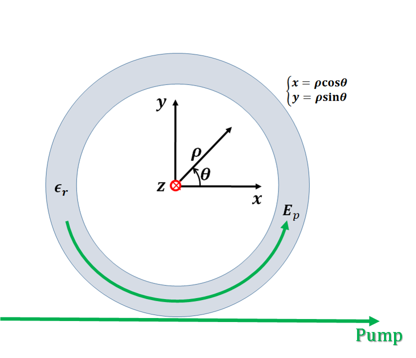
is the linear dielectric response of the medium in the time domain with due to causality, is the relative electric permittivity in the frequency domain, is the cubic nonlinearity, is the fraction of the pump field coupled with the resonator and acts as the source term, the pump frequency, is the electric permittivity at the pump frequency, and the speed of light in the vacuum. Eq. (A.1) is valid if we assume that the linear and nonlinear response of the material is local and isotropic and we also assume that the nonlinear response of the material is instantaneous. The assumption that the response is instantaneous corresponds physically to just considering the fast nonlinear electronic response of the medium and neglecting the contribution of the molecular vibrations (Raman effect) Agrawal ; Hasegawa1 . It is convenient to pass from the real to the complex field representation: and . With reference to Fig. 5, we can expand the complex electric field E by using the guided modes of the resonator in cylindrical coordinates as
|
|
|
(A.3) |
and we can expand as
|
|
|
(A.4) |
where the are the time-dependent envelope functions, labels the two families of transverse modes with amplitudes and , and eigenfrequencies and , is the polarization vector of the pump field, is the azimuthal angle and finally is the azimuthal number that labels the eigenfrequencies in each family. We note that, while we restrict our analysis here to two families of modes, our coupled mode theory can be extended to an arbitrary number of families.
The field profile solves the eigenmode equation
|
|
|
(A.5) |
subject to the orthonormality condition
|
|
|
(A.6) |
where is the elementary volume in cylindrical coordinates, is the volume occupied by the resonator, and is the Krönecker -function. In Eq. (A.5) we take into account the material as well as the waveguide dispersion, since we explicitly consider the electric permittivity as a function of frequency.
Expressing Eq. (A.1) in the complex field representation and using Eqs. (A.3) and (A.4), as well as the eigenmode equation, Eq. (A.5), and, finally, by invoking the slowly varying envelope approximation , the dot and double dot denote respectively the first and second time derivative, we arrive at the following equation, containing just the first order time derivatives of the envelope functions,
|
|
|
|
|
|
|
|
|
|
|
|
(A.7) |
where and
|
|
|
|
|
|
(A.8) |
|
|
|
|
|
|
(A.9) |
with and . From now on, we omit the dependence of the envelope functions on and the dependence of the field profiles on , and .
In order to arrive at coupled mode equations, we project Eq. (A.7) on the modes, and we use their orthonormality, which yields
|
|
|
|
|
|
|
|
|
|
|
|
|
|
|
(A.10.a) |
|
|
|
|
|
|
|
|
|
|
|
|
|
|
|
(A.10.b) |
We have introduced the following overlap integrals, involving just the transverse profile of the guided modes in the resonator ,
|
|
|
(A.11.a) |
|
|
|
(A.11.b) |
|
|
|
(A.11.c) |
The integration for the overlap integrals is extended only over the resonator volume because is zero outside the resonator, and is by definition the fraction of the pump field coupled with the resonator.
The coefficient is the effective field for the mode of the family , while the terms and are the effective nonlinear coupling coefficients, due respectively to the self-phase modulation (SPM) and the four-wave mixing (FWM) cubic nonlinearity. Equation (A.10) describes two nonlinear four-wave mixing processes. The first is due to the SPM cubic nonlinearity and has a frequency detuning given by for the families 1 and 2. The second is due to the FWM cubic nonlinearity and has a frequency detuning given by for the families 1 and 2. The detuning for both processes would be zero if the eigenfrequencies were equidistant, which would correspond to perfect phase matched interactions and infinite coherence length. In practice, the perfect phase matching condition is never fulfilled in WGM resonators where instead the deviation from equidistance of the eigenfrequencies plays a fundamental role, as we will show later. The effect of the finite bandwidth of the cavity modes has been taken into account in Eq. (A.10) by the phenomenological introduction of the decay terms into the equations, where is the photon lifetime in the cavity and is the bandwidth of the resonance.
Equation (A.10) is an exact representation of the electromagnetic problem stated in Eq. (A.1). However, the direct numerical integration of these coupled mode equations is computationally inefficient because it is necessary to integrate a system of equations, each one containing terms, and a microresonator typically contains to modes.
We now decouple the transverse field evolution from its azimuthal evolution by using only two dominant modes for the transverse field profile, one for each family, namely:
with where is the azimuthal number corresponding to the closest to the pump eigenfrequency for each family, i.e for . This approximation is justified because the dependence of the transverse field profile of a guided mode on the propagation wavevector—in our case on the azimuthal number —is usually weak. Hence, we may assume that the transverse profile is nearly the same as for the respective dominant modes. In this way, Eq. (A.3) can be rewritten in the following form
|
|
|
(A.12.a) |
where
|
|
|
(A.12.b) |
is the spatio-temporal envelope of the total field. By taking the partial time derivative of Eq. (A.12.b) we obtain:
|
|
|
|
|
|
(A.13) |
where the term can be expressed through a Taylor expansion as
|
|
|
(A.14) |
The coefficient is the free spectral range (FSR) of the resonator at the frequency and the coefficient equals, at lowest order, the deviation from equidistance of the eigenfrequencies adjacent to and plays a role analogous to the group velocity dispersion (GVD) of a standard optical fiber. In particular, corresponds to the normal dispersion regime in which the group velocity decreases for increasing frequencies, while corresponds to the anomalous dispersion. It is also customary to introduce the GVD parameter , so that the dispersion is normal when and anomalous when . Using a Taylor expansion of the term and the following identity
|
|
|
|
|
|
(A.15) |
we can recast Eq. (A.13) in the form
|
|
|
|
|
|
(A.16) |
where the time derivatives of the field envelopes in the the last term at the right-hand side can be explicitly calculated by using the coupled mode Eq. (A.10).
Our goal is to write Eq. (A.16) in a form that just includes envelope fields , so that we obtain coupled nonlinear wave equations for . In doing so, we make several approximations. First, we suppose that the decay times for all the modes of the same family are the same: . For high-Q WGM resonators, we generally have decay times on the order of and Q-factors given by .
Second, we suppose that, as is usual in nonlinear optical phenomena, the effects of the nonlinearity and of the pump on the envelope field occur on a much slower time scale than the time scale necessary for the field to complete one round-trip in the resonator. In a typical WGM resonator with radius, the round trip time is , while the time scale on which the nonlinearity and the pump field produce significant effects on the field envelope is in the or range. Hence, once the time derivative of the field envelopes is calculated using Eq. (A.10), the nonlinear terms and pump terms in Eq. (A.16) can be averaged over the azimuthal coordinate from to . Hence, all the terms proportional to , with , do not effectively contribute to the process because they average to zero and can be neglected. Third, we approximate the overlap integrals as follows: and , consistent with the weak dependence of the radial field profiles on the azimuthal number.
Moreover, in the pump term we simplify and , and we introduce the detuning of the pump field with respect to the dominant modes, . Fourth, we expand and around and keep only the lowest order. Finally, we collect the nonlinear terms oscillating with the same detuning and retain only the nonlinear terms whose frequency detuning vanishes, i.e., we only retain the frequency-matched terms . We then obtain two incoherently coupled, externally driven, damped, generalized NLSEs or LLEs
|
|
|
|
|
|
|
|
|
(A.17) |
where
|
|
|
|
|
|
(A.18) |
are the overlap integrals of the interacting modes. Note that . Equations (A.17) and (A.18) are our starting points, Eqs. (1) and (2).