Wolf-Rayet stars in the Small Magellanic Cloud

Abstract

Context. Massive Wolf-Rayet (WR) stars are evolved massive stars ($M_{\text{i}}\gtrsim 20\,M_{\odot}$) characterized by strong mass-loss. Hypothetically, they can form either as single stars or as mass donors in close binaries. About 40 % of the known WR stars are confirmed binaries, raising the question as to the impact of binarity on the WR population. Studying WR binaries is crucial in this context, and furthermore enable one to reliably derive the elusive masses of their components, making them indispensable for the study of massive stars.

Aims. By performing a spectral analysis of all multiple WR systems in the Small Magellanic Cloud (SMC), we obtain the full set of stellar parameters for each individual component. Mass-luminosity relations are tested, and the importance of the binary evolution channel is assessed.

Methods. The spectral analysis is performed with the Potsdam Wolf-Rayet (PoWR) model atmosphere code by superimposing model spectra that correspond to each component. Evolutionary channels are constrained using the Binary Population and Spectral Synthesis (BPASS) evolution tool.

Results. Significant Hydrogen mass fractions ($0.1<X_{\text{H}}<0.4$) are detected in all WN components. A comparison with mass-luminosity relations and evolutionary tracks implies that the majority of the WR stars in our sample are not chemically homogeneous. The WR component in the binary AB 6 is found to be very luminous ($\log L\approx 6.3\,[L_{\odot}]$) given its orbital mass ($\approx 10\,M_{\odot}$), presumably because of observational contamination by a third component. Evolutionary paths derived for our objects suggest that Roche lobe overflow had occurred in most systems, affecting their evolution. However, the implied initial masses ($\gtrsim 60\,M_{\odot}$) are large enough for the primaries to have entered the WR phase, regardless of binary interaction.

Conclusions. Together with the results for the putatively single SMC WR stars, our study suggests that the binary evolution channel does not dominate the formation of WR stars at SMC metallicity.

1 Introduction

Figure 1: Narrow band O [iii] nebular emission image of the SMC (Smith et al. 2005) with all known WR stars marked. Yellow stars correspond to confirmed binary systems.

Stars with initial masses $M\gtrsim 20\,M_{\odot}$ may reach the Wolf-Rayet (WR) phase, which is characterized by strong stellar winds and hydrogen depletion, at a late stage of their evolution as they approach the Eddington limit (Conti 1976). There are two prevalent channels for a star to do so. On the one hand, the powerful radiation-driven winds of massive stars can peel off their hydrogen-rich layers, which leads to the typical emission line WR spectrum (Castor et al. 1975; Cassinelli 1979). On the other hand, mass donors in binary systems may shed copious amounts of mass during Roche lobe overflow (RLOF), approaching the Eddington limit owing to severe mass-loss (e.g. Paczynski 1973). Several studies (e.g. Maíz Apellániz 2010; Sota et al. 2011; Sana et al. 2012; Chini et al. 2012; Aldoretta et al. 2015) give direct evidence that at least half of all massive stars are binaries. Among the WR stars, about $40\,\%$ are confirmed binaries (van der Hucht 2001). It is inevitable that some of these systems would contain interacting companions. Sana et al. (2013) estimate that roughly half of the O-type stars will interact with a companion via mass transfer during their lifetime, and recent studies invoke binary interaction to explain a multitude of phenomena (e.g. Vanbeveren et al. 2007; Richardson et al. 2011; Langer 2012; de Mink et al. 2013). Yet the impact of binarity on the WR population remains debated (e.g. Vanbeveren et al. 1998; Crowther 2007).

Binaries are not only important from an evolutionary standpoint; they further enable one to deduce stellar parameters to an accuracy unattainable for single stars. For instance, if the orbital inclination $i$ and both radial velocity (RV) curves can be obtained, the companions’ masses can be accurately calculated from Newtonian dynamics. This method is indispensable in the case of WR stars, whose masses are otherwise difficult to determine. Knowledge of these masses provides a critical test, not only of stellar evolution models, but also of mass-luminosity relations (MLRs) for WR stars (Langer 1989; Gräfener et al. 2011). Studies of wind-wind collisions (WWC) in massive binaries have proven fruitful for obtaining orbital inclinations (Luehrs 1997; Moffat 1998; Reimer & Reimer 2009). These types of wind collisions were also suggested to be prodigious X-ray sources (Cherepashchuk 1976; Prilutskii & Usov 1976), which was fully confirmed by subsequent observations and modeling efforts (e.g. Stevens et al. 1992; Zhekov 2012; Rauw & Naze 2015), and yielding important physical constraints on WR binaries.

Hence, there are various reasons why a spectroscopic and photometric analysis of WR binaries is essential for the study of massive stars. Despite this, binaries have often been left out in previous spectroscopic studies of WR stars (e.g. Hamann et al. 2006; Sander et al. 2012; Hainich et al. 2014) because of the complexity involved in their analysis. This paper begins to bridge the gap by presenting a systematic analysis of WR binaries.

An interesting test case for the impact of binarity on WR stars is offered by investigating low metallicity environments. Since the mass-loss rate $\dot{M}$ scales with surface opacity that originates in metals, it is expected to decrease with decreasing surface metallicity $Z$ (Kudritzki et al. 1987; Puls et al. 2000; Vink et al. 2000). For WR stars, recent empirical studies suggest $\dot{M}\propto Z$ (e.g. Nugis et al. 2007; Hainich et al. 2015). The smaller $Z$ is, the harder it is for a single star to develop the stellar wind necessary to become a WR star. Standard stellar evolution models predict that, at solar metallicity, initial masses of $M_{\text{i}}\gtrsim 20\,M_{\odot}$ are sufficient for single stars to reach the WR phase, while at a metallicity of about $0.1\,Z_{\odot}$, masses of at least $\sim 45\,M_{\odot}$ are required (Meynet & Maeder 2005). The frequency of single WR stars is thus expected to decrease with $Z$. In contrast, the frequency of WR stars formed via RLOF is not a priori expected to depend on $Z$.

Motivated by such predictions, Foellmi et al. (2003b), Foellmi, Moffat, & Guerrero (2003a, FMG hereafter), Schnurr (2008), and Bartzakos et al. (2001a) conducted a large spectroscopic survey in the Small and Large Magellanic Cloud (SMC and LMC, respectively) with the goal of measuring the binary fraction in their respective WR populations. The LMC and SMC are both known to have a subsolar metallicity: a factor $\sim 1/3$ and $\sim 1/7$ solar, respectively (Dufour et al. 1982; Larsen et al. 2000). Following the reasoning of the previous paragraph, it is expected that the fraction of WR stars formed via RLOF will be relatively large in the LMC, and even larger in the SMC. Bartzakos et al. (2001a) made use of stellar evolution statistics published by Maeder & Meynet (1994) to predict that virtually all WR stars in the SMC are expected to have been formed via RLOF. Similar predictions remain even with the most recent generation of stellar evolution codes (e.g. Georgy et al. 2015). It was therefore surprising that FMG measured a WR binary fraction in the SMC of $\sim 40\,\%$, consistent with the Galactic fraction, revealing a clear discrepancy between theory and observation which must be explained.

Table 1: Overview of the known WR stars in the SMC and their binary status

Object	Spectral Type	V [mag]	Binary status	$K_{1}$ [km ${\rm s}^{-1}$]	$K_{2}$ [km ${\rm s}^{-1}$]	$P$ [d]	$i$ [∘]	$e$
SMC AB 1	WN3ha	15.1	-	-	-	-	-	-
SMC AB 2	WN5ha	14.2	-	-	-	-	-	-
SMC AB 3	WN3h + O9	14.5	SB2	144	-	10.1	$57_{-29}^{+33}$	0.09
SMC AB 4	WN6h	13.3	-	-	-	-	-	-
SMC AB 5	(WN6h + WN6-7) + (O + ?)	11.1	SB3	214	200	19.3	$86^{+1}_{-1}$	0.27
SMC AB 6	WN4 + O6.5I:	12.3	SB2	290	66	6.5	$57^{+33}_{-12}$	0.1
SMC AB 7	WN4 + O6I(f)	12.9	SB2	196	101	19.6	$68^{+22}_{-15}$	0.07
SMC AB 8	WO4 + O4V	12.8	SB2	176	55	16.6	$40^{+10}_{-3}$	0
SMC AB 9	WN3ha	15.2	Uncertain	43	-	34.2	-	0.22
SMC AB 10	WN3ha	15.8	-	-	-	-	-	-
SMC AB 11	WN4ha	15.7	-	-	-	-	-	-
SMC AB 12	WN4(?)	15.5	-	-	-	-	-	-

Hainich et al. (2015, paper I hereafter) conducted a spectral analysis of the putatively single WR stars in the SMC. In the present paper, we perform a non-local thermodynamic equilibrium (non-LTE) analysis of the WR binary systems. Having derived the full set of parameters for all components of each system, we test current MLRs, and deduce evolutionary paths for each system.

The paper is structured as follows: Sects. 2 and 3 give an overview of our sample and the observational data used. In Sect. 4, we describe the assumptions and methods involved in the spectral analysis. In Sect. 5, we give the full set of stellar parameters derived, while Sect. 6 contains a thorough discussion and interpretation of our results. A summary of our results is found in Sect. 7. The appendices include a detailed description on the properties and analysis of our objects (A), their evolutionary paths (B), and their spectral fits (C).

2 The sample

There are 12 WR stars currently known in the SMC (Massey et al. 2014). Fig. 1 marks the positions of the known SMC WR stars on a narrow band image of the O [iii] nebular emission line. Five out of the 12 stars are in confirmed binary or multiple systems based on their RV curves (FMG), marked with yellow stars in Fig. 1. As in paper I, we follow the name scheme SMC AB # (sometimes simply AB #), as introduced by Azzopardi & Breysacher (1979). Table 1 gives an overview on the 12 WR stars currently known in the SMC and their binary status. All but one are WN (nitrogen rich) stars; the WO (oxygen rich) primary in AB 8 is the exception. For the binary systems, we give the two velocity amplitudes $K_{1}$ and $K_{2}$, periods $P$, orbital inclinations $i$, and eccentricities $e$, if known. For the quadruple system AB 5, the orbital parameters refer to the short period WR + WR binary within the system.

The adopted orbital inclination angles $i$ heavily affect the deduced orbital masses $M_{\text{orb}}$ ($M_{\text{orb}}\propto\sin^{3}i$). The inclinations of AB 5 and 8 could be constrained in other studies thanks to photospheric/wind eclipses. Since $i$ is the only free parameter determining the orbital masses in the case of AB 6 and 7, we use calibrations by Martins et al. (2005) to fix their inclinations so that the secondary’s orbital mass agrees with its spectral type. With both $i$ and $K_{2}$ unknown in the case of AB 3, we fix $i$ to its mean statistical value so that $\sin^{3}i=\left<\sin^{3}i\right>=3\,\pi/16$, and adjust $K_{2}$ to calibrate the secondary’s mass against its spectral type.

In all systems, we conservatively assume an uncertainty of no more than a factor two in the secondary’s orbital mass, and assume the realistic constraints $15\,M_{\odot}\leq M_{\text{O}}\leq 70\,M_{\odot}$ and $M_{\text{WR}}\geq 5\,M_{\odot}$ for the O and WR stars in the sample, respectively (e.g. Martins et al. 2005; Crowther 2007). If additional constraints on $i$ are known from other studies, they are considered as well. This restricts $i$ to a corresponding value range.

The binary candidate SMC AB 9 (cf. Table 1) is omitted from this analysis. The star was already analyzed as a single star in paper I because of the absence of any spectral features which could be associated with a companion in its spectrum. For the same reason, we treat SMC AB 5 (HD 5980) as a triple system, and not a quadruple. None of the spectral features are clearly associated with the fourth component, whose existence is anticipated based on a periodic variability of the absorption lines associated with the third component (Breysacher et al. 1982; Koenigsberger et al. 2014).

3 Observational data

3.1 Spectroscopic data

For three systems (AB 3, 6, and 7), we use normalized, low-resolution spectra ($\text{FWHM}\approx$ 2.8 – 6.7 Å) obtained by FMG in the spectral range of 3900–6800 $\AA$ between the years 1998 and 2002. Detailed information on the instrumentation used and the data reduction can be found in FMG. To obtain a relatively high Signal-to-Noise ratio (S/N) of about $100-150$, spectra taken at different binary phases were co-added in the frame of the primary. Although the reduced spectra used by FMG for RV studies are available for download, the online data suffer from obvious wavelength calibration problems for reasons that we could not trace. The original data could not be retrieved. Due to this and the poor S/N of the original spectra, we make use only of the co-added spectra in this study. Co-adding the spectra in the frame of the WR star causes the companion’s spectral features (an O star in these systems) to smear. Its lines would thus appear broader and shallower than they should, although their equivalent width remains conserved. To account for this effect, we convolve the companion’s model with a box function of the width $K_{1}+K_{2}$ when comparing to these spectra. Given the low resolution of the spectra, this effect is of secondary importance. If possible, auxiliary spectra were used to derive parameters which are sensitive to the line profile.

For all of our targets, we downloaded flux calibrated spectra taken with the International Ultraviolet Explorer (IUE) covering the spectral range $1200-2000\,\AA$ from the MAST archive. When available, high resolution spectra are preferred, binned at intervals of $0.05\,\AA$ to achieve an S/N$\approx 15$. Otherwise, low resolution spectra are used ($\text{FWHM}\approx 6\,\AA$, $\text{S/N}\approx 20$). Low resolution, flux calibrated IUE spectra in the range $2000-3000\,\AA$ are not used for detailed spectroscopy because of their low S/N ($\approx 5-10$), but rather to cover the spectral energy distribution (SED) of the targets. Optical low resolution spectra taken by Torres-Dodgen & Massey (1988) are also used for the SEDs of our targets. Flux calibrated, high resolution Far Ultraviolet Spectroscopic Explorer (FUSE) spectra covering the spectral range $960-1190\,\AA$ are also retrieved from the MAST archive and binned at $0.05\,\AA$ to achieve an $\text{S/N}\approx 30$, except for AB 3, for which no usable FUSE spectra could be obtained. The IUE and FUSE spectra are normalized with the reddened model continuum.

For AB 5, we use auxiliary flux calibrated, high resolution ($\text{FWHM}\approx 0.02\,\AA$) spectra taken in 2009 during primary eclipse ($\phi=0$) with the STIS instrument mounted on the Hubble Space Telescope (HST) covering the spectral range $1150-1700\,\AA$, with $\text{S/N}\approx 30$ (Koenigsberger et al. 2010). The spectra are also normalized using the model continuum. Unfortunately, no out-of-eclipse UV spectra taken after the year 1999 are available in the archives. For this system, we also retrieved several high resolution spectra taken in 2005 with the Fiber-Fed Extended Range Optical Spectrograph (FEROS) mounted on the MPI 2.2 m telescope at La Silla, covering the spectral range $3750-9200\,\AA$ at a resolution of $\text{FWHM}\approx 0.1\,\AA$ and $\text{S/N}\approx 40$. The data were reduced and used by Foellmi et al. (2008), where more information can be found. Additionally, we use a spectrum created by co-adding several spectra at phase $\phi=0$ to achieve a $\text{S/N}\approx 200$, made available by Foellmi et al. (2008).

For AB 8, we make use of a reduced, flux calibrated spectrum with a resolution of $\text{FWHM}\approx 0.2\,\AA$ and $\text{S/N}\approx 100$ taken with the X-shooter spectrograph mounted on ESO’s Very Large Telescope (VLT), covering the range $3000-25000\,\AA$ (Vernet et al. 2011). The reduced spectrum was kindly supplied to us by F. Tramper (see Tramper et al. (2013) for details).

The dates and ID numbers of all spectra used here are given in the figures showing them. Phases are calculated with ephemeris given by FMG, except for AB 8 and 5, where the ephemeris given by St-Louis et al. (2005) and Koenigsberger et al. (2014) are used, respectively. The spectral resolution is accounted for by convolving the models with corresponding Gaussians to mimic the instrumental profile.

3.2 Photometric data

Aside from flux-calibrated data, we use for all stars analyzed here $JHK$ and IRAC photometry from Bonanos et al. (2010). If available, we also use their $UBVRI$ magnitudes. For AB 5, we use the $U$ and $BVR$ magnitudes from Torres-Dodgen & Massey (1988) and Zacharias et al. (2005), respectively; For AB 6, we use UBV magnitudes from Mermilliod (1995); for AB 8, we use the UBV magnitudes from Massey (2002) and $I$ magnitude given by the DENIS Consortium (2005). For all stars, we use WISE magnitudes from Cutri & et al. (2013).

4 Non-LTE spectral modeling of WR binaries

4.1 The PoWR code

PoWR is a non-LTE model atmosphere code especially suitable for hot stars with expanding atmospheres. The code iteratively solves the co-moving frame radiative transfer and the statistical balance equations in spherical symmetry under the constraint of energy conservation. A more detailed description of the assumptions and methods used in the code is given by Gräfener et al. (2002) and Hamann & Gräfener (2004). By comparing synthetic spectra generated by the code to observations, a multitude of stellar parameters can be derived.

The inner boundary of the model, referred to as the stellar radius $R_{*}$, is defined at the Rosseland optical depth $\tau_{\mathrm{Ross}}$=20, where LTE can be safely assumed. In the subsonic region, the velocity field is defined so that a hydrostatic density stratification is approached (Sander et al. 2015). In the supersonic region, the pre-specified wind velocity field $v(r)$ generally takes the form of the $\beta$-law (Castor et al. 1975)

$$v(r)=v_{\infty}\left(1-\frac{r_{0}}{r}\right)^{\beta}.$$ (1)

Here, $v_{\infty}$ is the terminal velocity, and $r_{0}\approx R_{*}$ is a constant determined so as to achieve a smooth transition between the subsonic and supersonic regions.

Beside the velocity law and chemical composition, four fundamental input parameters are needed to define a model atmosphere: the effective temperature $T_{*}$, the surface gravity $g_{*}$, the mass-loss rate $\dot{M}$, and the stellar luminosity $L$. The effective temperature relates to $R_{*}$ and $L$ via the Stefan-Boltzmann law: $L=4\,\pi\,\sigma\,R_{*}^{2}\,T_{*}^{4}$. The gravity $g_{*}$ relates to the radius $R_{*}$ and mass $M_{*}$ via the usual definition: $g_{*}=g(R_{*})=G\,M_{*}R_{*}^{-2}$. For the vast majority of WR models, the value of $g_{*}$ bears no significant effects on the synthetic spectrum, which originates primarily in the wind. The outer boundary is taken to be $R_{\text{max}}=100\,R_{*}$ for O models and $1000\,R_{*}$ for WR models, which were tested to be sufficient.

During the iterative solution, the line opacity and emissivity profiles at each radial layer are Gaussians with a constant Doppler width $v_{\text{Dop}}$. This parameter is set to $30$ and $100\,$km ${\rm s}^{-1}$  for O and WR models, respectively. In the formal integration, the Doppler velocity is decomposed to depth-dependent thermal motion and microturbulence $\xi(r)$. We assume $\xi(r)$ grows with the wind velocity up to $\xi(R_{\text{max}})=0.1\,v_{\infty}$, and set $\xi(R_{*})=20$ km ${\rm s}^{-1}$  for O models and 100 km ${\rm s}^{-1}$  for WR models, respectively (e.g. Hamann et al. 2006; Bouret et al. 2012; Shenar et al. 2015). We assume a macroturbulent velocity of $30\,$km ${\rm s}^{-1}$  for all O components (e.g. Markova & Puls 2008; Bouret et al. 2012), accounted for by convolving the profiles with radial-tangential profiles (e.g. Gray 1975; Simón-Díaz & Herrero 2007).

It has become a consensus that winds of massive stars are not smooth, but rather clumped (Moffat et al. 1988; Lépine & Moffat 1999; Markova et al. 2005; Oskinova et al. 2007; Prinja & Massa 2010; Šurlan et al. 2013). An approximate treatment of optically thin clumps using the so-called microclumping approach was introduced by Hillier (1984) and systematically implemented by Hamann & Koesterke (1998), where the population numbers are calculated in clumps which are a factor of $D$ denser than the equivalent smooth wind ($D=1/f$, where $f$ is the filling factor).

Because optical WR spectra are dominated by recombination lines, it is customary to parametrize their models using the so-called transformed radius (Schmutz et al. 1989),

$$R_{\text{t}}=R_{*}\left[\frac{v_{\infty}}{2500\,{\rm km}\,{\rm s}^{-1}\,}\middle/\frac{\dot{M}\sqrt{D}}{10^{-4}\,M_{\odot}\,{\rm yr}^{-1}}\right]^{2/3},$$ (2)

defined such that equivalent widths of recombination lines of models with given $R_{\text{t}}$ and $T_{*}$ are approximately preserved, independently of $L$, $\dot{M}$, $D$, and $v_{\infty}$. While $R_{\text{t}}$ has the dimensions of length, it should be thought of as an integrated volume emission measure per stellar surface area.

4.2 Assumptions

PoWR models are limited to spherical symmetry, which obviously breaks down in the case of close binary systems. Firstly, the stars are deformed into a tear-like shape due to tidal forces. Secondly, non-spherical manifestations resulting from binary interaction, such as WWC cones or asymmetrical accretion flows, may occur in binary systems. While such phenomena may be significant or even dominant in the case of specific lines (e.g. Bartzakos et al. 2001b), they typically amount to flux variations of the order a few percent (e.g. Hill et al. 2000; Palate et al. 2013), with the possible exception of AB 5 (see Appendix A).

The detailed form of the velocity field in the wind domain can affect spectral features originating in the wind. WR models are therefore more sensitive to the velocity law than O-star models. The finite disk correction predicts a $\beta$-law (Eq. 1) in the case of OB-type stars with $\beta=0.8$ (e.g. Kudritzki et al. 1989), which we adopt for the O-star models. This value is consistent with analyses of clump propagation in O-type stars (e.g. Eversberg et al. 1998). As for WR stars, there are several empirical studies which suggest that the $\beta$ exponents in the outer winds of WR stars with strong winds are in excess of four (Lépine & Moffat 1999; Dessart & Owocki 2005). On the other hand, $\beta$ values of the order of unity are found for hydrogen rich WR stars (Chené et al. 2008), which describes most of our sample. For the WR components, we thus always assume the usual $\beta$-law with $\beta=1$.

The data do not always enable us to derive the chemical abundances for each element, in which case we assume the following. For the O companions, we adopt H, C, N, O, Mg, Si, and Fe mass fractions as derived for B stars in the SMC by Korn et al. (2000), Trundle et al. (2007), and Hunter et al. (2007): $X_{\text{H}}=0.73$, $X_{\text{C}}=2.1\cdot 10^{-4}$, $X_{\text{N}}=3.26\cdot 10^{-5}$, $X_{\text{O}}=1.13\cdot 10^{-3}$, $X_{\text{Mg}}=9.9\cdot 10^{-5}$, $X_{\text{Si}}=1.3\cdot 10^{-4}$, and $X_{\text{Fe}}=3\cdot 10^{-4}$. We scale the mass fractions of the remaining metals to 1/7 solar, in accordance with the ratio of the solar metallicity (Asplund et al. 2009) to the average SMC metallicity (Trundle et al. 2007): $X_{\text{Ne}}=1.8\cdot 10^{-4}$, $X_{\text{Al}}=7.6\cdot 10^{-6}$, $X_{\text{P}}=8.3\cdot 10^{-7}$, $X_{\text{S}}=4.4\cdot 10^{-5}$. The same mass fractions are adopted for WR models, except for $X_{\text{H}}$, which is derived in each case, and the CNO mass fractions, which are adopted as in paper I: $X_{\text{C}}=2.5\cdot 10^{-5}$, $X_{\text{N}}=1.5\cdot 10^{-3}$, $X_{\text{O}}=1.0\cdot 10^{-6}$.

A longstanding problem is assessing the density contrast in clumps and their stratification in the atmosphere. Here, $D(r)$ is assumed to be depth-dependent, increasing from $1$ (smooth wind) at the base of the wind to a maximum value $D$ (e.g. Owocki et al. 1988). Quite generally, allowing $D(r)$ to be depth-dependent yields more symmetric, less “self-absorbed” line profiles, as illustrated in Fig. 9 in the appendix. It is found that a depth dependent clumping factor which initiates from $D(R_{*})=1$ at the base of the wind and grows proportionally to the wind velocity to the value $D(r)=D$ at $v(r)\geq 0.5\,v_{\infty}$ provides a good agreement with the observations, which tend to exhibit symmetric profiles. The maximal value $D$ can be roughly constrained for each WR star (see Sect. 4.3), and is treated as a free parameter. We note that other studies suggest clumping may already initiate at the photosphere (e.g. Cantiello et al. 2009; Torrejón et al. 2015). Clumping factors for the O companions, which cannot be deduced from the available spectra, are fixed to $D=10$, supported by hydrodynamical simulations (Feldmeier et al. 1997). When the companions’ mass-loss rates cannot be constrained, we adopt them from hydrodynamical predictions by Vink et al. (2000).

We adopt a distance of $d=62$ kpc to the SMC (Keller & Wood 2006). The reddening towards our objects is modeled using a combination of the reddening laws derived by Seaton (1979) for the Galaxy, and by Gordon et al. (2003) for the SMC. As in paper I, we assume an extinction of $E_{B-V}=0.05$ for the Galactic component (Sect. 4.3 in paper I) and fit for the total extinction, adopting $R_{\text{V}}=3.1$.

4.3 The analysis method

The non-LTE analysis of spectra, even in the case of single stars, is an iterative and computationally expensive process. Generally, $g_{*}$ is inferred from the wings of photospheric H and He ii absorption lines. The effective temperature $T_{*}$ is inferred from the line ratios of ions belonging to the same element, mostly He lines for the O stars, and mostly metal lines for WR stars. Wind parameters such as $\dot{M}$ (or $R_{\text{t}}$) and $v_{\infty}$ are derived from recombination and P Cygni lines. If possible, the maximum density contrast $D$ is derived from electron-scattering wings. The luminosity $L$ and total extinction $E_{B-V}$ are determined by fitting the combined spectral energy distribution (SED) of the models to the photometric measurements. The abundances are determined from the overall strengths of lines belonging to the respective elements. Finally, the projected rotation velocity $v\sin i$ is constrained from profile shapes. For the O companions, this is done by convolving the models with appropriate rotation profiles. For the WR stars, if the resolution and S/N enable such an analysis, we derive upper limits for rotation by applying a 3D integration scheme, assuming co-rotation up to $\tau_{\text{Ross}}=2/3$ (Shenar et al. 2014).

Figure 2: Observed SED of AB 6 (blue lines and squares) compared to the synthetic SED (red dashed line), which is the sum of the WR (black solid line) and O (green dotted line) models.

Figure 3: Comparison between IUE (ID:sp41784, $\phi=0.47$) and optical (co-added, FMG) rectified spectra of SMC AB 6 (blue ragged line) and the composite synthetic spectrum (red dashed lines). The composite model is the sum of the WR (black solid line) and O (green dotted line) models. The relative offsets of the model continua correspond to the light ratio between the two stars. Note that the light ratios are different in the optical and UV due to the different temperatures of both components.

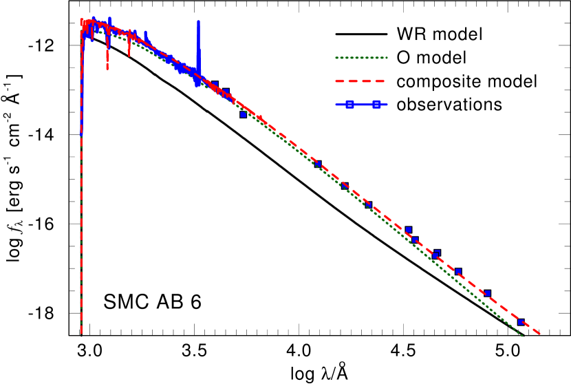
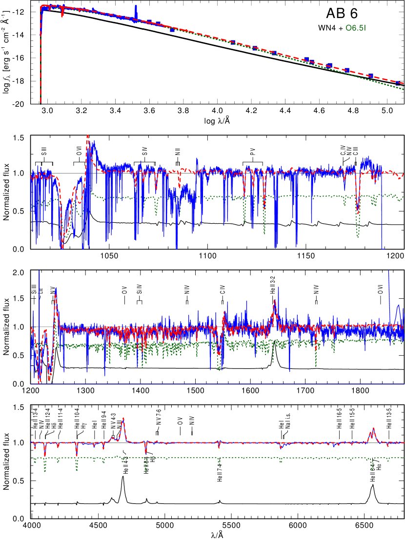
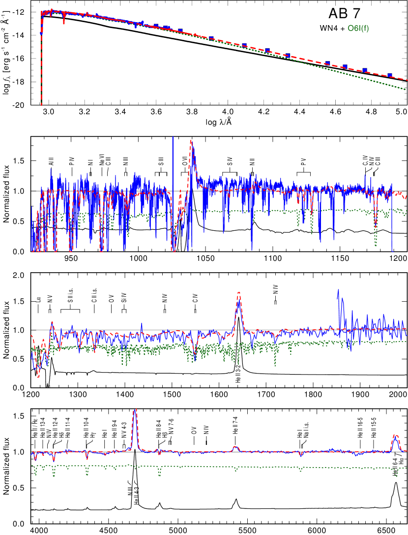
To analyze a multiple system, models for each of its components are required. Ideally, one would disentangle the composite spectrum to its constituent spectra by observing the system at different phases (e.g. Bagnuolo & Gies 1991; Hadrava 1995; Marchenko & Moffat 1998). Unfortunately, our data do not enable this. Moreover, spectral disentangling does not yield direct information regarding the light ratios unless the stellar system is eclipsing. Since we work with composite spectra, our task is therefore to combine models in such a way that the composite spectrum and SED are reproduced. An example is shown in Figs. 3 and 2, where a comparison between the SED and observed rectified spectra of the binary system SMC AB 6 and our best fitting models is shown, respectively.

As opposed to single stars, the luminosities of the components influence their relative contribution to the flux and thus the synthetic normalized spectrum. The light ratios of the different components therefore become entangled with the fundamental stellar parameters, and it is not trivial to overcome the resulting parameter degeneracy. The analysis of composite spectra thus consists of the following steps:

• Step 1: Based on line ratios and previous studies (e.g. spectral types), preliminary models for the O and WR companions are established. If necessary, the spectra are shifted to account for systemic/orbital motion.

• Step 2: The light ratios are derived (or constrained) by identifying absorption features which can be clearly associated with the O companion and which are preferably not sensitive to variations of its physical parameters. While identifying the WR lines is usually easier, their strengths strongly depend on the mass-loss rate and thus do not enable one to determine the light ratios independently.

• Step 3: The luminosity of one of the companions and the reddening of the system are adjusted to fit the available photometry. Since the light ratio is known/constrained, the luminosity of the companion follows.

• Step 4: $\dot{M}$ (or $R_{\text{t}}$), $D$, and $v_{\infty}$ are adjusted for the WR model based on the strengths of its lines.

• Step 5: If needed, the parameters of the WR and O models are further refined. If any wind lines can be associated with the O companion, its wind parameters are adjusted.

• Step 6: With the refined models, steps 2 - 5 are repeated until no significant improvement to the fit of prominent lines (at a few percent level) can be achieved.

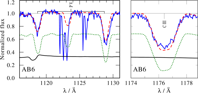
The set of spectral lines most diagnostic for the analysis generally depends on the system. In Fig. 4, we show an example for two photospheric features which originate in the secondary beyond doubt, and which greatly help to deduce the light ratio in the case of SMC AB 6: the P v $\lambda\lambda\,1118,1128$ resonance doublet (left panel) and the strong C iii multiplet at $\approx\lambda 1176$ (right panel). Optical He lines as well as the spectral type imply $30<T_{*}<40\,$kK for the secondary. A careful comparison of O star models in this temperature range reveals that these lines are insensitive to temperature and gravity variations. We thus conclude that the relative strength of such lines in the normalized spectrum is affected primarily by the light ratio. The features imply a similar light ratio of $F(\text{O})/F(\text{WR})\sim 2$ in the FUSE domain, and agree with the other features in the available spectra, e.g. sulfur lines. While this method is sensitive to the adopted abundances, $X_{\text{P}}$ and $X_{\text{S}}$ should remain fairly constant (e.g. Bouret et al. 2012) throughout the stellar evolution. A multitude of lines is used for each system to reduce the probability for a systematic deviation.

Figure 4: Comparison between the rectified FUSE observation of AB 6 (ID:X0150102000, $\phi=0.44$, blue ragged line) and the composite synthetic spectrum (red dashed line) for the P v $\lambda\lambda\,1118,1128$ resonance doublet and the C iii multiplet at $\sim\lambda 1176$. The WR and O models are depcited by a black solid line and green dotted line, respectively. The narrow absorption features originate in the interstellar medium (ISM).

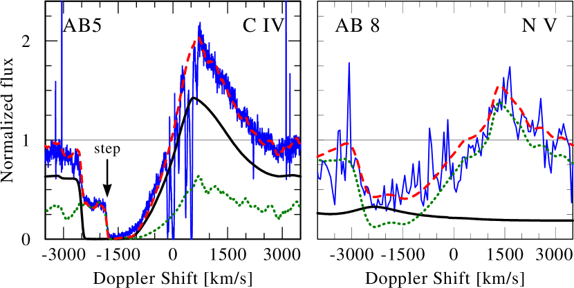
Another robust way for determining the light ratios is offered by high resolution P Cygni line profiles. An example is shown in the left and right panels of Fig. 5. The left panel shows a high resolution HST spectrum of the C iv resonance doublet of the quadruple system AB 5, taken at $\phi\cong 0$ during an eclipse of the secondary (B) by the primary (A). The spectrum clearly shows a P Cygni absorption consisting of two contributions originating in the primary and tertiary (C). As Georgiev et al. (2011) already demonstrated, the strength of the “step” observed in the C iv doublet is influenced by the components’ light ratio. The different terminal velocities of stars A and C cause the more extended part of the line to appear unsaturated. The right panel shows the N v resonance doublet $\lambda\lambda\,1239,1243$ for the WO binary AB 8, which clearly originates in the O companion and which is typically saturated in observations of single O stars with strong winds (e.g. Walborn 2008; Bouret et al. 2012), but is not saturated here because of light dilution by the WO component. Such features give sharp constraints on the light ratios.

Figure 5: Same as Fig. 4, but showing the observed C iv $\lambda\lambda\,1548,1551$ resonance doublet in AB 5 (HST, ID:ob2na1020, $\phi\cong 0$, left panel) and the observed N v resonance doublet $\lambda\lambda\,1239,1243$ in AB 8 (IUE, ID:sp07623, $\phi=0.79$, right panel) in velocity space relative to the respective blue components of each doublet. Colors are as in Fig. 4.

WR stars are almost always devoid of pure photospheric features and so their surface gravities cannot be determined via spectral analysis. Their gravities are fixed to $G\,M_{\text{orb}}\,R_{*}^{-2}$ throughout the analysis, after $R_{*}$ has been determined, but we note that the appearance of the WR spectra calculated here are virtually independent of $\log g$. Determining the gravity of the secondaries proved to be a hard task, leading to large errors in $\log g$. As described in Sect. 3, the co-added optical spectra of AB 3, 6, and 7 suffer from low resolution and a smearing of the companion’s features. However, while the profiles of the Balmer and He ii lines cannot be studied in detail because of the quality of the spectra, their equivalent widths grow with increasing $\log g_{*}$, which enabled its rough estimation.

In Appendix A, we give an overview on each analyzed system, supply a thorough documentation of the analysis, and highlight spectral features of notable interest.

Table 2: Inferred stellar parameters for the SMC WR binaries

	AB3		AB5			AB6		AB7		AB8
Component	A	B	A	B	C	A	B	A	B	A	B
Spectral type	WN3h	O9	WN6h	WN6-7	O	WN4	O6.5 I	WN4	O6 I(f)	WO4	O4 V
$T_{\ast}$ [kK]	$78^{+5}_{-5}$	$30^{+5}_{-5}$	$45^{+5}_{-5}$	$45^{+10}_{-7}$	$34^{+3}_{-3}$	$80^{+15}_{-10}$	$37^{+3}_{-3}$	$105^{+20}_{-10}$	$36^{+3}_{-3}$	$141^{+60}_{-20}$	$45^{+5}_{-5}$
$T_{2/3}$ [kK]	$77^{+5}_{-5}$	$30^{+3}_{-5}$	$43^{+5}_{-5}$	$43^{+10}_{-7}$	$33^{+3}_{-3}$	$78^{+15}_{-10}$	$37^{+3}_{-3}$	$98^{+20}_{-10}$	$35^{+3}_{-3}$	$115^{+10}_{-10}$	$44^{+5}_{-5}$
$\log g_{*}$ [cm s-2]	$4.3$	$3.9^{+0.3}_{-0.3}$	$3.5$	$3.5$	$3.2^{+0.2}_{-0.2}$	$3.7$	$3.5^{+0.2}_{-0.2}$	$4.7$	$3.6^{+0.2}_{-0.2}$	$5.1$	$4.0^{+0.3}_{-0.3}$
$\log L$ [$L_{\odot}$]	$5.93^{+0.05}_{-0.05}$	$4.5^{+0.2}_{-0.2}$	$6.35^{+0.10}_{-0.10}$	$6.25^{+0.15}_{-0.15}$	$5.85^{+0.10}_{-0.10}$	$6.28^{+0.10}_{-0.10}$	$5.90^{+0.10}_{-0.10}$	$6.10^{+0.10}_{-0.10}$	$5.50^{+0.10}_{-0.10}$	$6.15^{+0.10}_{-0.10}$	$5.85^{+0.10}_{-0.10}$
$\log R_{\text{t}}$ [$R_{\odot}$]	$1.07^{+0.05}_{-0.05}$	-	$1.15^{+0.05}_{-0.05}$	$1.3^{+0.1}_{-0.1}$	-	$1.2^{+0.1}_{-0.1}$	-	$0.75^{+0.10}_{-0.10}$	-	$0.40^{+0.05}_{-0.05}$	-
$v_{\infty}/10^{3}$ [km ${\rm s}^{-1}$]	$1.5^{+0.1}_{-0.1}$	$2.0^{+0.5}_{-0.5}$	$2.2^{+0.2}_{-0.2}$	$2^{+0.5}_{-0.5}$	$1.65^{+0.1}_{-0.1}$	$2.2^{+0.2}_{-0.2}$	$2.0^{+0.2}_{-0.2}$	$1.7^{+0.2}_{-0.2}$	$1.5^{+0.3}_{-0.3}$	$3.7^{+0.3}_{-0.3}$	$3.2^{+0.3}_{-0.3}$
$R_{*}$ [$R_{\odot}$]	$5^{+1}_{-1}$	$7^{+6}_{-3}$	$24^{+10}_{-7}$	$22^{+15}_{-10}$	$24^{+8}_{-6}$	$7^{+3}_{-2}$	$22^{+7}_{-5}$	$3.4^{+1.2}_{-1.2}$	$14^{+5}_{-3}$	$2^{+1}_{-1}$	$14^{+6}_{-4}$
$R_{2/3}$ [$R_{\odot}$]	$5^{+1}_{-1}$	$7^{+6}_{-3}$	$26^{+10}_{-7}$	$23^{+15}_{-10}$	$25^{+8}_{-6}$	$7^{+3}_{-2}$	$22^{+7}_{-5}$	$4.0^{+1.4}_{-1.4}$	$15^{+5}_{-3}$	$3^{+1}_{-1}$	$15^{+6}_{-4}$
$D$	$10^{+10}_{-5}$	$10$	$40_{-20}$	$10$	$10$	$10^{+10}_{-5}$	$10$	$10^{+10}_{-5}$	10	$40_{-20}$	10
$\log\dot{M}$ $[M_{\odot}\,{\rm yr}^{-1}]$	$-5.3^{+0.1}_{-0.1}$	$-8.0$	$-4.5^{+0.1}_{-0.1}$	$-4.5^{+0.3}_{-0.3}$	$-5.9$	$-5.1^{+0.2}_{-0.2}$	$-5.8$	$-5.0^{+0.2}_{-0.2}$	$-7.0^{+0.3}_{-0.5}$	$-4.8^{+0.1}_{-0.1}$	$-6.1^{+0.5}_{-0.3}$
$v\sin i$ [km ${\rm s}^{-1}$]	-	$200^{+100}_{-100}$	$<300$	$<400$	$120^{+30}_{-30}$	-	$150^{+50}_{-50}$	-	$150^{+30}_{-30}$	-	$120^{+20}_{-20}$
$v_{\text{eq}}$ [km ${\rm s}^{-1}$]	-	$240_{-140}^{+300}$	$<300$	$<400$	$120^{+30}_{-30}$	-	$180^{+100}_{-80}$	-	$160_{-30}^{+70}$	-	$190^{+40}_{-60}$
$M_{V,\text{John}}$ [mag]	$-4.4^{+0.2}_{-0.2}$	$-3.6^{+0.5}_{-0.5}$	$-7.1^{+0.3}_{-0.3}$	$-6.8^{+0.4}_{-0.4}$	$-6.7^{+0.3}_{-0.3}$	$-5.15^{+0.3}_{-0.3}$	$-6.65^{+0.3}_{-0.3}$	$-4.4^{+0.3}_{-0.3}$	$-5.7^{+0.3}_{-0.3}$	$-4.9^{+0.3}_{-0.3}$	$-5.9^{+0.3}_{-0.3}$
$X_{\rm H}$ (mass fr.)	0.25${}^{+0.05}_{-0.05}$	0.73	0.25${}^{+0.05}_{-0.05}$	0.25${}^{+0.20}_{-0.20}$	0.73	0.4${}^{+0.1}_{-0.1}$	0.73	0.15${}^{+0.05}_{-0.05}$	0.73	$0^{+0.15}$	0.73
$X_{\rm C}/10^{-5}$ (mass fr.)	$2^{+1}_{-1}$	$21$	$3^{+1}_{-1}$	$3^{+2}_{-2}$	$21$	$3^{+1}_{-1}$	$21$	$3^{+1}_{-1}$	$21$	$0.30^{+0.05}_{-0.05}\cdot 10^{5}$	$21$
$X_{\rm N}/10^{-3}$ (mass fr.)	$4^{+2}_{-2}$	$0.03\,(|\,1)$	$2.5^{+1}_{-1}$	$2.5^{+1}_{-1}$	$0.03$	$3^{+1}_{-1}$	$0.03\,(|\,0.3)$	$2^{+1}_{-1}$	$0.03\,(|\,0.3)$	0	0.03
$X_{\rm O}/10^{-5}$ (mass fr.)	$5.5$	$110$	$5.5$	$5.5$	$110$	$5.5$	$110$	5.5	110	$0.3^{+0.1}_{-0.1}\cdot 10^{5}$	$110$
$E_{B-V}$ [mag]	0.18${}^{+0.01}_{-0.01}$		0.08${}^{+0.02}_{-0.02}$			0.065${}^{+0.01}_{-0.01}$		0.08${}^{+0.01}_{-0.01}$		0.07${}^{+0.01}_{-0.01}$
$A_{V}$ [mag]	0.56${}^{+0.03}_{-0.01}$		0.25${}^{+0.06}_{-0.06}$			0.20${}^{+0.03}_{-0.03}$		0.25${}^{+0.03}_{-0.03}$		0.22${}^{+0.03}_{-0.03}$
$M_{\rm H-b}$ [$M_{\odot}$]	$46^{+7}_{-6}$	-	$83^{+20}_{-16}$	$73^{+42}_{-25}$	-	$101^{+30}_{-23}$	-	$51^{+13}_{-10}$	-	-	-
$M_{\rm He-b}$ [$M_{\odot}$]	$29^{+2}_{-2}$	-	$54^{+9}_{-9}$	$47^{+13}_{-10}$	-	$49^{+9}_{-7}$	-	$37^{+6}_{-5}$	-	$40^{+7}_{-6}$	-
$M_{\rm g}$ [$M_{\odot}$]	-	$13^{+70}_{-10}$	-	-	$34^{+64}_{-22}$	-	$54^{+97}_{-34}$	-	$30^{+55}_{-19}$		$70^{+210}_{-52}$
$M_{\rm orb}$ [$M_{\odot}$]	$20^{+80}_{-15}$	$20^{+20}_{-5}$	$61^{+10}_{-10}$	$66^{+10}_{-10}$	-	$9^{+7}_{-3}$	$41^{+29}_{-16}$	$23^{+13}_{-5}$	$44^{+26}_{-9}$	$19^{+3}_{-8}$	$61^{+14}_{-25}$
$R_{\text{RL}}[R_{\odot}]$	$25^{+29}_{-6}$	$25^{+11}_{-6}$	$58^{+4}_{-4}$	$60^{+4}_{-4}$	-	$14^{+3}_{-2}$	$28^{+9}_{-7}$	$40^{+8}_{-3}$	$54^{+13}_{-6}$	$33^{+3}_{-5}$	$57^{+7}_{-12}$

5 Results

Table 2 summarizes the stellar parameters derived for the components of the five systems analyzed. The spectral fits are available in Appendix C (Figs. 11 to 16). The Table also includes the temperatures and radii at $\tau_{\text{Ross}}=2/3$, H, C, N, O abundances, Johnson $V$ magnitudes, projected and equatorial rotation velocities $v\sin i$ and $v_{\text{eq}}$, total reddenings $E_{B-V}$ and extinctions $A_{V}$, and Roche lobe radii $R_{\text{RL}}$, calculated from the orbital masses using the Eggleton approximation (Eggleton 1983). We also give several types of stellar masses: $M_{\text{H-b}}$ and $M_{\text{He-b}}$ are derived for WR stars from MLRs calculated by Gräfener et al. (2011) for chemically homogeneous core H- and He-burning stars, respectively (see Sect. 6.1). $M_{\rm g}=G^{-1}\,g_{*}\,R_{*}^{2}$ is inferred from the derived surface gravity. Finally, $M_{\rm orb}$ denotes the orbital masses, calculated from the orbital parameters given in Table 1.

Uncertainties for the fundamental stellar parameters are estimated by examining the sensitivity of the fits to changes in the corresponding parameters. These include errors on $T_{*}\,,\log g_{*}\,,\log L,\log R_{\text{t}},v_{\infty},D,E_{\rm B-V},v\sin i$ and abundances. Error propagation is used for the remaining parameters. Errors on $\dot{M}$ include only errors on $R_{\text{t}}$. Errors on $M_{\text{orb}}$ are dominated by errors on $i$ (cf. Table 1), except for AB 5, where the uncertainty on the orbital solution dominates (Koenigsberger et al. 2014).

6 Discussion

6.1 Comparison with mass-luminosity relations

The surface of WR stars remains hidden behind their stellar winds, rendering a determination of their masses via photospheric absorption lines or astroseismological methods difficult. The only method to estimate the masses of single WR stars is by using mass-luminosity relations (MLRs, e.g. Langer 1989; Gräfener et al. 2011). Clearly, these relations need to be calibrated with model-independent methods for measuring stellar masses. Binary systems offer the most reliable method to ”weigh” stars using simple Newtonian dynamics, given that the required observables ($K_{1},K_{2},P,i$, and $e$) are known.

We now compare theoretical MLRs published by Gräfener et al. (2011) to the luminosities and orbital masses inferred for the WR primaries in our sample. The relations are calculated for the simplified case of chemically homogeneous stars. In these relations, $\log L$ is given as a second order polynomial in $\log M$ (see Eqs. 9 and 10 in Gräfener et al. 2011), where the coefficients depend on the hydrogen mass fraction $X_{\text{H}}$. In these relations, if $X_{\text{H}}>0$, the star is assumed to be core H-burning. Otherwise, it is assumed to be core He-burning.

For a star with a given luminosity, the largest possible mass predicted by theory is obtained for chemically homogeneous, hydrogen burning stars (Eq. 11 in Gräfener et al. 2011). Lower masses are obtained if the star has a He-burning core. Gräfener et al. (2011) argue that the MLR derived for pure helium stars (Eq. 13 in Gräfener et al. 2011) should give a good approximation for the masses of evolved, He-burning WR stars. However, if the contribution of shell H-burning to the luminosity is significant, a given luminosity can be supported by a yet smaller mass. The most strict lower bound on the mass at a given luminosity is given by the classical Eddington limit calculated for a fully ionized atmosphere (including only electron scattering).

Fig. 6 compares the theoretical predictions of the MLRs to the empirically derived $(M_{\text{orb}},\log L)$ coordinates for the WR companions. The Eddington limit, calculated for a fully ionized helium atmosphere, is also plotted. Langer (1989) also provides calculations for homogeneous stars with a vanishingly small helium abundance, which may be more suitable for the WO component in AB 8. Since these calculations predict a very similar relation to the MLR calculated for pure He-stars (the latter predicting slightly lower luminosities for a given mass), we omit the corresponding MLR from Fig. 6 for clarity.

Figure 6: Positions of the WR components on a $M-\log L$ diagram (symbols) compared to MLRs calculated for homogeneous stars (Gräfener et al. 2011), depicted by solid curves. The colors correspond to the hydrogen content (see legend). The Eddington limit calculated for a fully ionized helium atmosphere is also plotted (gray dashed line).

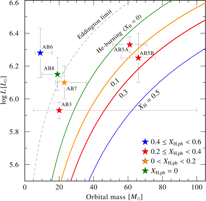
Both massive WR components of AB 5 are located between MLRs calculated with $X_{\text{H,core}}=0$ and $0.3$. This suggests that these stars may still be core H-burning, although both could coincide with the relation for He-burning stars within errors. Since the WR components of AB 3, 7, 6, and 8 are of early spectral type, which are understood to be core He-burning stars, we can expect them to lie on the MLR for pure He-stars, or, if a significant fraction of the luminosity originates in shell burning, between this relation and the Eddington limit. As is apparent in Fig. 6, these stars do lie above the pure He-star MLR, suggesting that they are indeed core helium burning. The WR component in AB 3 is poorly constrained due to the large error on $M_{\text{orb}}$. Since all analyzed WN components show signatures of hydrogen in their atmospheres, this suggests that the majority of WR stars in our sample are not chemically homogeneous. Taken at face value, their offsets from the MLR calculated for pure helium stars suggests the presence of shell H-burning (or shell He-burning in the case of AB 8).

While the WR component of AB 7 is located below the Eddington limit, that of AB 8 (WO) slightly exceeds it. The internal structure of WO stars is poorly understood and hard to model (N. Langer, priv. com.). Regardless, it should not be possible for the star to exceed the Eddington limit, unless significant departures from spherical symmetry occur already in the stellar interior (e.g. Shaviv 2000). However, considering the given errors on $\log L$ and $M_{\text{orb}}$, there is no clear discrepancy in the case of AB 8.

The only star in the sample for which a clear inconsistency is obtained is the WR component of the shortest-period binary in our sample, AB 6. The star clearly exceeds its Eddington limit, which immediately implies that the derived luminosity and/or the orbital mass are incorrect. Furthermore, we find a significant amount of hydrogen ($\approx 40\%$) in its atmosphere, which is not expected for highly evolved, He-burning stars. In Sect. 6.4, we discuss possible reasons for this discrepancy, and argue that the orbital mass derived for the WR companion is most likely wrong. It is therefore omitted when considering the evolutionary status of the system in the next sections.

6.2 Evolutionary status: avoiding mass-transfer due to homogeneous evolution

Given the short orbital periods of our objects, it seems likely that the primaries underwent a RLOF phase before becoming WR stars. However, rapid initial equatorial rotation in excess of $400\,$km ${\rm s}^{-1}$  (Heger et al. 2000; Brott et al. 2011) may lead to quasi-chemically homogeneous evolution (QCHE). A star experiencing QCHE maintains higher effective temperatures and thus much smaller radii throughout its evolution, and may therefore avoid overfilling its Roche lobe during the pre-WR phase.

In paper I, we argued that the properties of the single SMC WR stars are compatible with QCHE. Yet tidal forces in binaries act to synchronize the axial rotation of the components with the orbital period (Zahn 1977). In binaries of extremely short periods ($\lesssim 2\,$d), synchronization can maintain, or even enforce, near-critical rotation of the components (e.g. de Mink et al. 2009; Song et al. 2016). However, none of the binaries in our sample portray such short orbital periods, and we find no evidence for a significant increase of the orbital period throughout their evolution (see Sect. 6.3). In our sample, tidal interactions are rather expected to have slowed down the stellar rotation. For example, for an O star of $10-20\,R_{\odot}$ (a typical main sequence WR progenitor), synchronization with the period of AB 5 (19.3 d) would imply a rotational velocity of only 50-100 km ${\rm s}^{-1}$. Even for AB 6, the shortest period binary in our sample (6.5 d), synchronization implies $150-300$ km ${\rm s}^{-1}$, which is insufficient to induce QCHE.

Table 3: Initial parameters and ages derived from single-star tracks assuming inhomogeneous evolution for the primary

	Inhomogeneous primaries, single-star tracks
SMC AB	3		5		6		7		8
$M_{\text{1,\,i}}[M_{\odot}]$	50		100		80		70		80
Age [Myr]	4.6		3.0		3.4		3.7		3.6
$R_{\text{max, 1}}[R_{\odot}]$	1800		1200		2000		2100		2000
$M_{\text{i,\,2}}[M_{\odot}]$	15		100		46		35		50
$v_{\text{rot,\,i,\,2}}$[km ${\rm s}^{-1}$]	230		-		170		160		130
$\log\left(T_{1}^{\text{E}}/T_{1}^{\text{O}}\right)$	-0.01	(0.03)	-0.01	(0.05)	-0.01	(0.06)	-0.02	(0.04)	0.09	(0.15)
$\log\left(L_{1}^{\text{E}}/L_{1}^{\text{O}}\right)$	-0.08	(0.08)	-0.04	(0.13)	-0.16	(0.15)	-0.07	(0.12)	-0.09	(0.13)
$M_{1}^{\text{E}}-M_{1}^{\text{O}}$	2	(50 )	-13	(14)	-	-	8	(14)	8	(10 )
$X_{\text{H,1}}^{\text{E}}-X_{\text{H,1}}^{\text{O}}$	-0.03	(0.05)	-0.11	(0.05)	-0.25	(0.1)	-0.03	(0.05)	0.00	(0.05)

Table 4: Initial parameters and ages derived from single-star tracks assuming homogeneous evolution for the primary

	Homogeneous primaries, single-star tracks
SMC AB	3		5		6		7		8
$M_{\text{i,\,1}}[M_{\odot}]$	50		70		100		50		70
Age [Myr]	4.5		3.4		2.2		5.4		4.6
$R_{\text{1,\,max}}[R_{\odot}]$	10		13		19		10		13
$M_{\text{i,\,2}}$	15		70		55		No solution		40
$v_{\text{rot\,i,\,2}}$	230		-		170		No solution		410
$\log\left(T_{1}^{\text{E}}/T_{1}^{\text{O}}\right)$	-0.12	(0.03)	0.13	(0.05)	-0.13	(0.06)	0.01	(0.06)	0.09	(0.15)
$\log\left(L_{1}^{\text{E}}/L_{1}^{\text{O}}\right)$	0.06	(0.08)	-0.13	(0.13)	0.05	(0.16)	-0.08	(0.12)	-0.08	(0.13)
$M_{1}^{\text{E}}-M_{1}^{\text{O}}$	28	(80 )	6	(11)	-	-	10	(10 )	8	(10 )
$X_{\text{H,1}}^{\text{E}}-X_{\text{H,1}}^{\text{O}}$	-0.03	(0.05)	-0.01	(0.05)	-0.03	(0.1)	-0.15	(0.05)	0.00	(0.05)

Synchronization timescales $\tau_{\text{sync}}$ involve much uncertain physics. Hurley et al. (2002) give some estimates for binary stars with a mass ratio $q=1$ and for initial masses up to $M_{\text{i}}=10\,M_{\odot}$. They show that for stars with $M_{\text{i}}>1\,M_{\odot}$ (i.e. stars with radiative envelopes), separations of the order of $10\,R_{*}$ ensure a synchronization timescale $\tau_{\text{syn}}$ which is smaller than the main sequence timescale $\tau_{\text{MS}}$, with the ratio $\tau_{\text{syn}}/\tau_{\text{MS}}$ virtually independent of the mass. Since the systems analyzed here are characterized by separations of a few $R_{*}$, tidal interactions are expected to have greatly lowered the initial rotation rates.

To test whether single-star evolutionary tracks can explain the observed properties of our objects, we compare the primaries’ $T_{*},L,M_{\text{orb}}$, and $X_{\text{H}}$ with evolutionary tracks for single stars with initial masses between $20\,M_{\odot}$ and $120\,M_{\odot}$ calculated at a metallicity of $Z=0.004$ with the BPASS (Binary Population and Spectral Synthesis) stellar evolution code (Eldridge et al. 2008, Eldridge et al. in prep.), which can treat both single and binary stars. We use two sets of tracks, one calculated assuming no chemical mixing, and the other calculated assuming a homogeneous evolution (Eldridge et al. 2011; Eldridge & Stanway 2012). For each WR star in our sample, we look for a track defined by $M_{\text{i}}$, and for an age $t$, which reproduce the observed quantities $T_{*},L,M_{\text{orb}}$ and $X_{\text{H}}$ as good as possible, in the sense of minimizing the sum

$$\chi^{2}\left(M_{\text{i}},t\right)=\sum_{n=1}^{4}\left(\frac{\text{O}_{n}-\text{E}_{n}\left(M_{\text{i}},t\right)}{\sigma_{n}}\right)^{2},$$ (3)

where $\text{O}_{n}\in\left\{\log T_{*},\log L,M_{\text{orb}},X_{\text{H}}\right\}$ are the inferred values for the considered observables, and $\text{E}_{n}\left(M_{\text{i}},t\right)$ are the corresponding predictions of the evolutionary track defined by the initial mass $M_{\text{i}}$ at age $t$. Only in the case of AB 6, we ignore the WR component’s orbital mass because of its clear inconsistency with the derived stellar luminosity (see Sects. 6.1 and 6.4). Since the tracks evolve non linearly, we avoid interpolation over the grid. Instead, we define $\sigma_{n}=\sqrt{\Delta_{n}^{2}+\delta_{n}^{2}}$, where $\Delta_{n}$ is half the $n$’th parameter’s grid spacing, and $\delta_{n}$ is the corresponding error given in Table 2. In the case of asymmetrical errors in Table 2, we assign $\delta_{n}$ according to whether $\text{O}_{n}>\text{E}_{n}$ or $\text{O}_{n}<\text{E}_{n}$. By minimizing $\chi^{2}$, we infer initial masses and ages for the primaries in the cases of no mixing and homogeneous evolution. Conservative uncertainties on the ages are constrained from the adjacent tracks in the vicinity of the solution (typically $0.2\,$Myr).

Figure 7: HRD positions of the all known single (paper I) and binary (this paper) SMC WR stars. The big symbols correspond to the binaries analyzed here, while circled smaller symbols correspond to putatively single stars. Plotted are evolutionary tracks (Eldridge et al. 2008) calculated for single stars at a metallicity of $Z=0.004$ assuming no mixing (left panel) and chemically homogeneous evolution (right panel). The colors and symbols code the hydrogen abundance and WR type, as described in the legend. The WR phase is defined at $X_{\text{H}}<0.6$. Tracks which correspond to the solutions found are shown in color.

As a second step, we test whether the ages derived are consistent with the current evolutionary status of the secondary, assuming still that no interaction has occurred between the companions. For this purpose, we use the BONNSAI Bayesian statistics tool (Schneider et al. 2014). The tool interpolates over detailed evolutionary tracks calculated by Brott et al. (2011) for stars of initial masses up to $60\,M_{\odot}$ and over a wide range of initial rotation velocities $v_{\text{rot, i}}$. Using $T_{*},L,M_{\text{orb}},v\sin i$ derived for the secondary, as well as the age derived for the primary (along with their corresponding errors), the algorithm tests whether a model exists which can reproduce the secondary’s properties at the derived age at a $5\%$ significance level. In case no such model was found, we verified this is not a consequence of the uncertain evolution of $v_{\text{eq}}$ by lifting the $v\sin i$ constraint. For AB 5, we use the BPASS tracks to check consistency with the secondary, since its mass is not covered by the BONNSAI tool.

Tables 3 and 4 show the initial masses $M_{\text{i,1}}$ and ages inferred for the primaries in the cases of inhomogeneous/homogeneous evolution. The Tables also give the maximum radius reached by the primary along the best-fitting track, $R_{\text{max, 1}}$. If consistent solutions for the secondaries are found by the BONNSAI tool, the secondaries’ initial masses $M_{\text{i, 2}}$ and rotations $v_{\text{rot, i}}$, as obtained from the BONNSAI tool, are given. Tables 3 and 4 also gives the differences $\text{O}_{n}-\text{E}_{n}$ for each of the primary’s parameters, where we also include $\sigma_{n}$ values. While all solutions provided by the BONNSAI reproduce the observed properties of the secondaries at a 5% significance level (Schneider et al. 2014), they do not do so equally well. However, since this is merely a consistency test for single-star evolution, we do not present a detailed description of the BONNSAI fit quality, which can be recovered online by the interested reader.

The two panels of Fig. 7 show the positions of the complete SMC WR population in a $\log L-\log T_{*}$ diagram (HRD), as derived in paper I and in this study. The left panel includes BPASS tracks for the primaries calculated assuming no mixing, while the right panel includes BPASS tracks assuming homogeneous evolution. The obtained solutions are highlighted in color. Note that the HRD contains only partial information regarding the fit quality (see Tables 3 and 4). For clarity, we do not include error bars in Fig. 7.

From this test, it seems that QCHE is not consistent with AB 3, 6, and 7. For example, the $T_{*}$ predicted by the track best fitting AB 3 deviates by 4$\sigma$ from our measurement. For AB 7, not only the hydrogen content is underpredicted, but also, the age is not consistent with the secondary’s stellar parameters. Based on our results, QCHE does not seem consistent with AB 5 either, since the temperature of the primary is overpredicted by more than $2\sigma$. However, Koenigsberger et al. (2014) manage to explain the evolutionary status of AB 5 by assuming non-interacting companions experiencing QCHE. This discrepancy occurs because of the lower value inferred for $T_{*}$ in this work compared to that used by Koenigsberger et al. (2014). Indeed, WWC in AB 5 may be responsible for a systematic uncertainty on $T_{*}$ (see Appendix A). Of all systems, only AB 8 is compatible with homogeneous evolution.

The tracks which do not include mixing generally show a better agreement. However, the primary stars in this set of evolutionary tracks reach radii which greatly exceed their Roche lobe radii (cf.  Table 3). If the systems did not undergo QCHE, there is little doubt that their companions have interacted via mass-transfer. In the next section, we account for this effect by considering binary evolution models.

6.3 Evolutionary status: assessing binary effects

Figure 8: Derived HRD positions of the WR components compared to the binary evolution tracks which best reproduce the set of eight observables (see text). The tracks shown correspond to the primary component. Colors are as in Fig. 7. The circles denote the best-fitting position (ages) along the tracks. RLOF phases are marked with dotted gray lines.

We would now like to compare the HRD positions of the binary systems to evolutionary tracks which account for binary interaction. modeling the evolution of binaries is difficult, because on top of the complex physics involved in the evolution of single stars, the effects of tidal interaction and mass-transfer have to be accounted for. While codes exist which account for these effects simultaneously (e.g. Cantiello et al. 2007), there are no corresponding grids of tracks available. Here, we make use of evolutionary tracks calculated with Version 2.0 of the BPASS code, which accounts for mass-transfer. The tracks do not include rotationally induced mixing or tidal interaction. However, as discussed in Sect. 6.2, mixing should be negligible for the majority of our objects. If mixing does become important in a binary system, its components will likely avoid RLOF, as can be inferred from the small radii maintained by the homogeneous models (cf.  Table 4). In this case, the solutions found from the single-star, chemically homogeneous evolutionary tracks should be adequate to describe the system.

Each binary track is defined by a set of three parameters: the initial mass of the primary $M_{\rm i,1}$, the initial orbital period $P_{\text{i}}$, and the mass ratio $q_{\text{i}}=M_{\text{i,2}}/M_{\text{i,1}}$. The tracks are calculated at intervals of $0.2$ on $0<\log P\,[\text{d}]<4$, $0.2$ on $0<q_{\text{i}}<0.9$, and at unequal intervals of $10-30\,M_{\odot}$ on $10<M_{\text{i,1}}<150\,M_{\odot}$. Again, we use a $\chi^{2}$ minimization algorithm to find the best-fitting track for each system. However, this time we consider eight different observables, thus leading to

$$\chi^{2}\left(P_{\text{i}},q_{\text{i}},M_{\text{i,\,1}},t\right)=\sum_{n=1}^{8}\left(\frac{\text{O}_{n}-\text{E}_{n}\left(P_{\text{i}},q_{\text{i}},M_{\text{i,1}},t\right)}{\sigma_{n}}\right)^{2},$$ (4)

where $\text{O}_{n}\in\left\{\log T_{1},\log L_{1},\log T_{2},\log L_{2},M_{\text{orb,\,1}},M_{\text{orb,\,2}},\log P,\right.$ $\left.X_{\text{H, 1}}\right\}$ are the measured values for the considered observables, and $\text{E}_{n}\left(P_{\text{i}},q_{\text{i}},M_{\text{i,1}},t\right)$ are the corresponding predictions of the evolutionary track defined by $P_{\text{i}}$, $q_{\text{i}}$, and $M_{\text{i,1}}$ at time $t$. $\sigma_{n}$ is defined as in Eq. 3.

Table 5: Comparison with the best fitting binary evolutionary tracks

SMC AB	3		5		6		7		8
$M_{\text{i,\,1}}[M_{\odot}]$	60		150		100		80		150
$q_{\rm i}(M_{\text{i,\,2}}/M_{\text{i,\,1}})$	0.3		0.5		0.5		0.5		0.3
$P_{\text{i}}$[d]	40		16		6		40		10
Age [Myr]	3.9		2.6		3.0		3.4		3.0
$\log\left(T_{1}^{\text{E}}/T_{1}^{\text{O}}\right)$	0.00	(0.03)	-0.02	(0.05)	-0.01	(0.06)	-0.02	(0.08)	0.09	(0.15)
$\log\left(L_{1}^{\text{E}}/L_{1}^{\text{O}}\right)$	-0.03	(0.08)	0.16	(0.13)	-0.03	(0.16)	-0.03	(0.12)	-0.11	(0.13)
$\log\left(T_{2}^{\text{E}}/T_{2}^{\text{O}}\right)$	0.08	(0.09)	-0.02	(0.07)	0.04	(0.08)	0.08	(0.08)	-0.06	(0.08)
$\log\left(L_{2}^{\text{E}}/L_{2}^{\text{O}}\right)$	0.09	(0.33)	-0.17	(0.26)	-0.16	(0.28)	0.03	(0.28)	-0.22	(0.27)
$M_{1}^{\text{E}}-M_{1}^{\text{O}}$	6	(50 )	26	(18)	-	-	11	(14 )	7	(10 )
$M_{2}^{\text{E}}-M_{2}^{\text{O}}$	-2	(16 )	31	(18)	30	(30)	-1	(14 )	10	(20 )
$\log\left(P^{\text{E}}/P^{\text{O}}\right)$	0.11	(0.10)	-0.07	(0.10)	0.02	( 0.1)	0.03	(0.1 )	0.02	(0.10)
$X_{\text{H,1}}^{\text{E}}-X_{\text{H,1}}^{\text{O}}$	-0.03	(0.05)	-0.03	(0.05)	-0.25	(0.1)	-0.01	(0.05)	0.00	(0.05)

The two panels in Fig. 8 show the best-fitting evolutionary tracks corresponding to the primary components along with their HRD positions. The circles correspond to the current positions (ages) derived. We stress, however, that the HRD illustrates only three of the eight observables which were fit here. In Table 5, we give the set of initial parameters defining the best-fitting tracks and ages found for each system, along with the differences $\text{O}_{n}-\text{E}_{n}$ and the corresponding uncertainties $\sigma_{n}$. Evidently, we manage to find tracks which reproduce the eight observables within a 2$\sigma$ level for all systems except AB 6. An evolutionary scenario which includes mass-transfer thus appears to be consistent with AB 3, 5, 7, and 8, although AB 8 was also consistent with QCHE. In Appendix B, we give a thorough description of the evolution of each system as given by the corresponding best-fitting track.

The solution for AB 5 overpredicts the components’ masses by almost 2$\sigma$, and is generally very sensitive to the weighting of the different observables (e.g.  small changes in $\sigma_{n}$). However, we believe this is simply a result of the grid spacing (see Appendix B). A greater challenge lies in explaining the similar hydrogen abundances of the two components The BPASS code does not follow the hydrogen abundance of the secondary, but since the two components were born with quite different masses in the derived solution ($150$ and $75\,M_{\odot}$), it is unlikely that they would evolve to a state of significant hydrogen depletion simultaneously. A conceivable resolution within the framework of binary evolution could involve the secondary losing much of its hydrogen envelope by undergoing a non-conservative RLOF, but this would likely require some fine tuning of the initial conditions. The QCHE scenario thus appears more natural in the case of AB 5, as proposed by Koenigsberger et al. (2014). However, it is not clear whether this scenario is consistent with the presence of tidal forces in the system. We discuss this system thoroughly in Appendix B.

As for AB 6, even when omitting the primary’s orbital mass in the fitting procedure, we obtain a $\approx 2.5\sigma$ discrepancy in the hydrogen abundance, which is found to be lower in the evolutionary track. However, our tests show that this discrepancy is lifted when using tracks which assume a lower metallicity ($Z=0.002$), i.e. this is a direct result of the uncertain mass-loss rates during the WR phase. Moreover, the BPASS binary models do not evolve the secondary in detail and therefore do not include the secondary overfilling its Roche lobe to transfer material back to the primary, as was reported for other stars (e.g. Groh et al. 2008). Such a process could contribute to the large amount of hydrogen detected in the WR star, although one would need to account for the secondary (which is observed to be an O-type supergiant) not entering the WR phase as a result of mass-loss during RLOF.

All binary solutions found go through a RLOF phase before the primary reaches the WR phase, which could already be anticipated given the large radii reached by the primaries after leaving the main sequence (cf.  Table 3). As discussed in Appendix B, RLOF typically removes $\approx 30\,M_{\odot}$ from the primary, at times partially accreted by the secondary. Mass transfer thus appears to be crucial for the detailed evolution of the systems which do not experience QCHE.

Despite the importance of mass-transfer, our results indicate that binary interaction does not contribute to the existing number of WR stars in the SMC. In Sect. 1, we argued that it is a priori expected that the majority (if not all) of the SMC WR population would stem from binary evolution, which generally enables WR stars to form at lower initial masses ($M_{\text{i}}\gtrsim 20\,M_{\odot}$) compared with single stars ($M_{\text{i}}\gtrsim 45\,M_{\odot}$). And yet, the initial masses of the primaries are found to be in excess of $60\,M_{\odot}$. This means that all WR components had large enough initial masses to become WR stars regardless of binary effects.

It is conceivable that the limit of $M_{\text{i}}\approx 45\,M_{\odot}$ for SMC stars to become WR stars is an overestimation, as it strictly holds for non-homogeneous stars. This limit can decrease to $\approx 20\,M_{\odot}$ if homogeneous evolutionary tracks are considered (cf. Fig. 7). Regardless, it is unclear why no WR binaries with intermediate-mass (20 - 40$\,M_{\odot}$) primary progenitors are found. Since the initial mass function strongly favors the formation of lower mass stars (Kroupa 2001), one would expect to see at least some WR binaries originating from intermediate-mass progenitors. The only WR stars in the SMC which imply intermediate-mass progenitors are the putatively single stars AB 2 and 10. As showed in Paper I, their HRD positions can be reproduced by assuming QCHE. Alternatively, they could stem from binary evolution. While the lack of confirmed companions sheds doubts on this scenario, post-RLOF binaries would often appear as single stars due to their small typical velocity amplitudes and/or the large brightness contrast of the companions (de Mink et al. 2014). The apparent lack of detected WR stars which are a direct result of binary interaction could thus be due to an observational bias.

Various studies (e.g. Packet 1981; Shara et al. 2015) suggest that the secondary should be spun up to near-critical rotation velocities as a consequence of mass accretion during the primary’s RLOF. Interestingly, all O-companions are found to have $v_{\text{eq}}$ values above the average for single O stars ($\approx 100\,$km ${\rm s}^{-1}$, e.g. Penny 1996; Ramírez-Agudelo et al. 2013), yet none of them are near critical ($\approx 500\,$km ${\rm s}^{-1}$). The fact that the O companions rotate with velocities above average implies that RLOF may have occurred, but the fact that they are sub-critical challenges this scenario. A resolution could lie in tidal interactions and/or mass-loss, which together lead to a rapid loss of angular momentum. Alternatively, the spin up during RLOF may be overestimated.

6.4 The strange case of AB 6

The system SMC AB 6 stands out as very enigmatic. In Sect. 6.1, we showed that the luminosity and orbital mass inferred for the WR component of AB 6 imply that it greatly exceeds its Eddington limit within errors. This means one or more of the following: (a) The parameters derived for the system in this paper, most importantly $\log L$, are incorrect; (b) The orbital mass derived by FMG is incorrect.

In Appendix A, we thoroughly describe how the components’ luminosities are derived. One caveat is that the method relies on the adopted abundances. Since we use different elements (C, S, P), and since not all are expected to change with evolution, a systematic deviation is unlikely. Furthermore, the light ratio cannot be very different than derived here, since a reduction of the WR luminosity would imply an unrealistic increase of the companion’s luminosity (e.g. Martins et al. 2005). However, a third component could contaminate the spectra. quite a few examples exist for false analyses of triple systems which were considered to be binary (e.g. Moffat & Seggewiss 1977). The immediate neighborhood of AB 6 is crowded with luminous stars and unresolved sources, which increases the probability for a third component contributing to the total light of the system. A third component could lead to a smaller luminosity for the WR component, although it would be hard to account for the $\approx 1$ dex downwards revision in $\log L$ which would be necessary to compensate for the discrepancies.

Another possibility is that the orbital mass is incorrect. To obtain a mass which fits more reasonably with our results, an inclination of $\sim 30^{\circ}$ would be required. However, assuming that the mass ratio derived by FMG is correct, such an inclination would also imply a mass of $\sim 170\,M_{\odot}$ for the O companion, which is unrealistic. Alternatively, it is possible that the actual mass ratio is different: The RV curve of the O component in AB 6 shown by FMG is based on noisy data points obtained from the motion of the absorption features in the low resolution optical spectra. A larger RV amplitude for the O star could lead to a larger orbital mass for the WR component. Moreover, a potential third source would not only affect the derived luminosities, but could also affect the RV measurements of the other two components (see e.g. Moffat & Seggewiss 1977; Mayer et al. 2010).

Although this short-period binary is a potential candidate for unique behavior patterns, its properties, as given here, are impossible to explain within the frame of binary evolution. This peculiar system should clearly be subject to further studies.

7 Summary

This study presented a systematic spectroscopic analysis of all five confirmed WR multiple systems in the low metallicity environment of the SMC. Together with Paper I, this work provides a detailed non-LTE analysis of the complete SMC WR population. We derived the full set of stellar parameters for all components of each system, and obtained important constraints on the impact of binarity on the SMC WR population.

Mass-luminosity relations (MLRs) calculated for homogeneous stars (Gräfener et al. 2011) reveal a good agreement for the very massive components of SMC AB 5 (HD 5980). Because of the errors on $\log L$ and $M_{\text{orb}}$, it is difficult to tell whether these stars are core H-burning or He-burning, although their derived positions are more consistent with core H-burning. The remaining WN stars in our sample show higher luminosities than predicted by the MLR calculated for pure He stars, implying core He-burning and shell H-burning (shell He-burning for the WO component in AB 8). This is consistent with the fact that all WN components show traces for hydrogen in their atmospheres ($0.1<X_{\text{H}}<0.4$).

The WO component in AB 8 is found to slightly exceed its Eddington limit, but this is likely a consequence of the errors on $\log L$ and $M_{\text{orb}}$. The small orbital mass ($\approx 10\,M_{\odot}$) and high luminosity ($\log L\approx 6.3\,[L_{\odot}]$) inferred for the WR component of AB 6 imply that it greatly exceeds its Eddington limit, which is clearly unphysical. We believe that the most likely resolution is an underestimation of the orbital mass, possibly because of a third component contaminating the spectrum of the system, which could also affect the derived luminosity. Overall, the positions of the WR stars in our sample on the $M-L$ diagram (Fig. 6), together with the derived atmospheric chemical compositions, suggest that the stars are not chemically homogeneous, with the possible exception of AB 5.

A comparison of the observed properties of each system to evolutionary tracks calculated with the BPASS and BONNSAI tools for chemically homogeneous/non-homogeneous single stars suggests that chemically homogeneous evolution (QCHE) is not consistent with four of the five systems analyzed (AB 3, 5, 6, and 7). In the case of AB 5, this is a direct result of the temperature derived in this study, which could be biased by the effects of wind-wind collisions (WWC), hindering us from a definite conclusion in its case. There are good reasons to believe that the components of AB 5 did in fact experience QCHE, but not without open problems (see Sect. 6.3 and Appendix B). The case of AB 8 is uncertain, as QCHE can explain its evolutionary state, although it is not a necessary assumption. This stands in contrast to the putatively single SMC WR stars, which are generally better understood if QCHE is assumed. The difference presumably stems from tidal synchronization, inhibiting an efficient chemical mixing in the stars. We showed that, if QCHE is avoided, the components of all our analyzed systems had to have interacted via mass-transfer in the past.

Mass-transfer in binaries is found to strongly influence the detailed evolution of the SMC WR binaries, significantly changing and redistributing the total mass of the system. That said, stellar winds too play a significant role in determining the final masses of the components, which stresses the importance of accurate mass-loss calibrations in evolutionary codes.

Despite the importance of mass-transfer, initial masses derived for the primaries are in excess of $60\,M_{\odot}$, well above the lower limit for single stars to enter the WR phase at SMC metallicity. Put differently, it seems that the primaries would have entered the WR phase regardless of binary effects. This suggests that the existing number of WR stars in the SMC is not increased because of mass transfer, in agreement with the fact that the observed WR binary fraction in the SMC is 40 %, comparable with the MW. No WR binaries are found with intermediate-mass ($20-40\,M_{\odot}$) progenitors, although their existence is predicted by stellar evolution models. Since post-RLOF systems tend to appear as single stars, this could be due to an observational bias.

The sample clearly suffers from low number statistics, and so any general claims put forth in this paper should be taken with caution. Our understanding of binary effects on the evolution of massive stars is expected to improve in the near future, as the sample of analyzed WR binaries will continue to grow. Meanwhile, our results should serve as a beacon for stellar evolution models aiming at reproducing the observed statistical properties of the plethora of massive stellar objects, to which WR stars belong.

Appendix A Comments on individual targets

In the few paragraphs below, we give a short overview on each system, and discuss specific issues related to their analysis. We also include an overview of the X-ray properties of each system.

AB 3: This system is classified as WN3h + O9 and is found to have a period of $P=10.0\,$d (Moffat 1988, , FMG). An X-ray source (CXOU J004959.4-732211) was detected in the close vicinity of AB 3 by both Chandra and XMM-Newton at a separation of $2.9^{\prime\prime}$. Within position uncertainties, the source could coincide with AB 3. If so, the X-ray luminosity of AB 3 is $L_{\rm X}\approx 2\times 10^{33}$ erg $\text{s}^{-1}$.

The spectrum is clearly dominated by the WR component; He i lines belonging to the secondary are only barely visible. The light ratio could be roughly constrained using the temperature-insensitive Balmer lines, and the implied luminosity obtained for the O companion suggests it is an O9 dwarf. The temperature of the WR star could be fairly well constrained due to the clear signatures of the C iv resonance doublet in the UV and the strong N v features in the optical, as well as the weak N iv features. $R_{\text{t}}$, $v_{\infty}$ and $D$ follow by fitting the strengths and shapes of the emission lines. We find a significant hydrogen content in the primary’s atmosphere.

Figure 9: Two models corresponding to the WR model of AB 3 (cf. Table 2) with a constant clumping factor $D(r)=D=10$ (black dotted line) and a depth-dependent clumping factor, where $D(R_{*})=1$ and $D(r)=10$ at $v(r)\sim 0.5\,v_{\infty}$ (black dashed line) compared to observations (blue solid line). We note that the O model contributes very little to these lines and is therefore omitted from this figure for clarity.

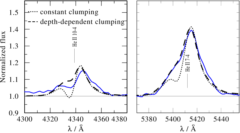
The emission visible at $\lambda\sim 4640$ probably corresponds to the N iii doublet $\lambda\lambda\,4634,4640$. No WR models are capable of reproducing this emission simultaneously with the N iv and N v features. It could only be reproduced by assuming higher temperatures and lower gravities for the O companion, and an extremely high N abundance, of the order of 30 times the SMC value. The potential nitrogen enrichment is given as an alternative $X_{\text{N}}$ value in Table 2. Alternatively, this feature could arise from WWC (e.g. Rauw et al. 1999). The companion’s terminal velocity is roughly estimated based on the shape of the badly resolved C iv resonance doublet, while the mass-loss rate is adopted from Vink et al. (2000).

AB 5: This strongly variable quadruple system, also known as HD 5980, contains four companions: an eclipsing binary system composing two WR stars (A:WNN6h + B:WN6-7) with a period of $P=19.3$ d, and another, probably distant binary system (C: O7 I + ?), responsible for distinct and relatively static absorption features in the spectrum (Breysacher et al. 1982; Niemela 1988; Koenigsberger et al. 2010, 2014). Here, we treat star C as a single star, since the fourth component is not noticeable in the spectrum, and therefore should not influence our results. The primary star went through a powerful LBV-type eruption in the year 1994. Since the eruption, the primary gradually increased in temperature from $\sim 25$ to $\sim 50$ kK, while its mass-loss rate has been gradually decreasing from $\sim 10^{-3.7}$ to $\sim 10^{-4.4}\,M_{\odot}\,{\rm yr}^{-1}$, and the terminal velocity increasing from $\sim 500$ to $\sim 2400$ km ${\rm s}^{-1}$(Georgiev et al. 2011). The system is the most X-ray luminous WR star in the SMC, with an X-ray luminosity $L_{\rm X}\approx 10^{34}$ erg ${\rm s}^{-1}$. Orbital variations in its X-ray flux were reported and could be explained by WWCs between the components A and B (Nazé et al. 2007). AB 5 is a prominent candidate for producing a massive black hole binary system such as recently detected by LIGO via gravitational waves (Abbott et al. 2016; Marchant et al. 2016).

Georgiev et al. (2011) presented a thorough analysis of the stars A and C at different epochs since the 1994 eruption, taking advantage of the fact that, at least for optically thick lines, the eclipse at phase $\phi=0$ (star A in front of star B) can be assumed to be full (Perrier et al. 2009). In our analysis, we use only the most recent spectra available. While the spectra taken during primary eclipse were taken at different epochs between the years 2002 and 2009 (see caption of Fig. 12), the system was stable during this period (Georgiev et al. 2011), so fitting them simultaneously is justified. Using the same approach as Georgiev et al. (2011) to isolate the stars A and C during the eclipse of B ($\phi=0$), we find similar parameters for both stars, although our solution implies a lower temperature for the primary ($T_{*}=$45 kK vs. 60 kK). Stars of subtype WN6h can have temperatures ranging between these values (e.g. Hamann et al. 2006).

We note that we neglect the effects of WWC here. Moffat (1998) claim that the phase-dependent width of the strongest optical emission lines is dominated by WWC during the eruptive era. Since the eruption, the primary’s mass-loss has significantly decreased, so WWC are now not expected to be as dominant, but could still contribute to the spectrum. Indeed, we find the strong He ii $\lambda 4686$ line is broader at maximal width (quadrature) than can be reproduced by a superposition of two WR stars with the given velocity amplitudes. This does not hold for the weaker He ii and nitrogen lines, partly because they form closer to the stellar surface, as Koenigsberger et al. (2014) noted. While He ii $\lambda 4686$ could be contaminated by WWC, our results do not depend on this line. However, WWC could potentially influence the strong He i $\lambda 5876$ line, which was used to constrain $T_{*}$ and $\dot{M}$. The discrepancy in $T_{*}$ could therefore be partly due to WWC.

We can only perform a rough analysis of the out-of-eclipse spectra, since the most recent publicly available observations covering the range $1200-2000\,\AA$ were taken in 1999, closer to the eruption. We thus rely on previous analyses as much as possible. Perrier et al. (2009) performed a quantitative analysis of the system’s light curve taken in 1979, before the 1994 eruption, and derived helpful constraints. They found that the relative contributions of stars A, B, and C in 1979 are approx. 0.4, 0.3, and 0.3 in the visual, respectively. Foellmi et al. (2008) present a comparison between this light curve and newer light curves taken in the years 2005 and 2006. While Foellmi et al. (2008) noted some interesting differences between the pre- and post-eruption light curves, the global behavior and strengths of flux minima during eclipse are virtually unchanged. This implies that the results published by Perrier et al. (2009) hold now as well. Furthermore, the fact that both primary and secondary minima are of very similar strengths implies that stars A and B have very similar temperatures. The clear appearance of N iv and N v lines which can be attributed to both components in the out-of-eclipse spectra confirms this. With the parameters of stars A and C fixed and the temperature of star B fixed to that of star A, the visual light ratios derived by Perrier et al. (2009) imply the luminosity of star B, and thus its radius. Finally, with these parameters fixed, we analyze the available out-of-eclipse spectra to derive the secondary’s wind parameters. Applying a 3D integration technique (Shenar et al. 2015), an upper limit on the components’ $v\sin i$ can be constrained using the N iv $\lambda 4058$ line, which forms very close to the stellar surface and is thus sensitive to surface rotation.

AB 6: With a period of $P=6.5\,$d, this SB2 WR + O binary system, classified WN4 + O6.5 I by FMG, is the shortest period WR binary known in the SMC (Moffat 1982; Hutchings et al. 1984). Despite its short period, the system shows no significant photometric variability. AB 6 was detected in the XMM-Newton survey (Laycock et al. 2010; Sturm et al. 2013) with an X-ray luminosity of $L_{\rm X}\approx 7\times 10^{33}$ erg $\text{s}^{-1}$ (in the 0.2-4.5 keV band). The source was found to be variable, with the $L_{\text{X}}$ reaching a peak of $\approx 10^{34}$ erg s^-1.

The luminosity of the WR component turns out to be very high, a fact which is not easy to explain given its orbital mass (see Sect. 6.1). Since this is a direct result of the derived light ratio, we briefly discuss its determination. The light ratio was derived on the basis of mainly three features: The P v $\lambda\,1128$ and S iv $\lambda 1073$ resonance lines, as well as the C iii $\lambda 1176$ multiplet, all of which are observed in the FUSE domain (see Fig. 4).

Moreover, while we do not identify a ”step” in the C iv resonance line (as in AB 5, see Fig. 5), it is clearly unsaturated at all phases, suggesting that it originates in only one of the binary components. We argue that this line originates in the O star. In Fig. 10, we show two HST spectra at $\phi=0.21$ (red line) and $\phi=0.77$ (blue line), as well as one IUE spectrum at $\phi=0.45$ (green line) in velocity space relative to the blue component of the C iv resonance doublet ($\lambda 1548$). The spectra are shifted by $-200\,$km ${\rm s}^{-1}$  to account for the systemic velocity of the system (FMG). While the line shows significant variability whose origin should be subjected to further study, no obvious radial velocity variation with phase can be seen in the line. If the line originates in the WR component, there should be a difference of roughly $500$ km ${\rm s}^{-1}$  between the velocities of the lines at phases $\phi=0.21$ and $\phi=0.73$, but no shift is observed. While emission lines need not strictly follow the orbital motion, some shift would be expected at such an RV amplitude. We conclude that this line originates in the O star, whose RV amplitude is $\sim 4$ times smaller, and that the WR star does not show this line at all, as is typical for early WN stars. This line helps us determine the light ratio as well, and puts constrains on the wind parameters of the O star. Lastly, the light ratio is consistent with He i and Balmer absorption lines in the optical spectrum.

As in AB 3, we find a clear signature of N iii $\lambda 4640$, which is very unlikely to originate in the WR component given its spectral class and derived temperature; indeed, we could not produce N v at its observed strength simultaneously to any N iii features. To reproduce it, an N-enrichment of roughly ten times the typical SMC value is assumed in the model of the O component, noted as an alternative value in Table 2. This feature could also originate in WWC, however.

Figure 10: Two HST spectra taken in 1992 (red line: Z0Z30402T, $\phi=0.21$, blue line: Z0Z30602T, $\phi=0.73$) and an IUE spectrum taken in 1991 (green line, sp41784, $\phi=0.45$) are plotted, showing the C iv resonance doublet of AB 6 in velocity space relative to the blue component at $\lambda 1548$.

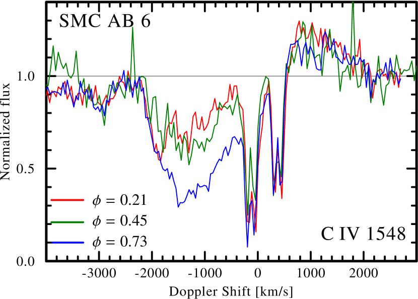
AB 7: Classified as WN4 + O6 I(f), this SB2 binary has a detected period of $P=19.6$ d (FMG). The system was also observed with XMM-Newton and is found to have a smaller X-ray luminosity than that of AB 6 ($L_{\rm X}\approx 4\times 10^{33}$ erg $\text{s}^{-1}$), which is also found to be variable (Guerrero & Chu 2008). Interestingly, although the mass-loss rates of WR stars in the SMC are on average lower than in those of their Galactic counterparts, the colliding wind SMC binaries (AB 5, 6, and 7) do not appear to be weaker X-ray sources than the Galactic ones. This suggests that the components’ mass-loss rates and the resulting X-ray luminosities may be related in a non-trivial way, or may even be uncorrelated (e.g. Ignace et al. 2000).

The temperature of the WR component is hard to constrain; The N v resonance line at $\lambda 1240$ is visible, but could in principle arise in both companions. There is a clear signature of N iii, but Niemela et al. (2002) associate it with the O companion based on RV shifts, and there are no N iv lines observed. Very weak N v lines in the optical can be seen, and suggest that the WR companion is indeed hot and suffers from strong line dilution, similar to AB 6. To avoid strong N v lines in the optical (which are not observed), one could either reduce the N abundance to abnormally low values (roughly a factor $0.3$ times the abundance given in Table 2), or increase the temperature to $\sim 10^{5}$ K, where the N v lines become very weak (because of dominance of the N vi ion). The latter solution provides a better fit to the available data.

Most peculiarly, the C iv resonance line only shows a narrow absorption, likely blended with interstellar absorption. For this reason, this line cannot help us to deduce the light ratio. As in the case of AB 6, we use the P v $\lambda\,1128$ and S iv $\lambda 1073$ resonance lines, as well as the C iii $\lambda 1176$ multiplet to constrain the light ratio, and derive the remaining parameters for both components based on the strengths of He i and He ii lines in the optical. To reproduce the unusual C iv feature (or, more accurately, lack thereof), we assume a low mass-loss rate for the O-star companion, and include X-rays in its model such that the total X-ray luminosity observed in this system is reproduced. The X-rays strongly depopulate the C iv ground state via Auger ionization.

As in the case of AB 3 and 6, the N iii emission excess at $\lambda 4640$ can be reproduced if a nitrogen abundance of roughly a factor 10 times the typical SMC abundance is assumed in the secondary. In fact, Niemela et al. (2002) showed that the feature roughly follows the orbital velocity of the O companion. We thus find possible signatures for nitrogen enrichment in SMC AB 3, 6, and 7. If true, this can be a consequence of either contamination by the primaries’ nitrogen-rich winds, or accretion during the primaries’ RLOF. Alternatively, this feature could originate in colliding winds, which are likely present in all of these systems.

AB 8: This system contains the only non-WN star known among the SMC WR sample. It was reclassified several times, most recently as WO4 + O4 V by Bartzakos et al. (2001a). Moffat et al. (1985) inferred an orbital period of $P=16.6$ d for the system. Interestingly, AB 8 is the only WR binary in our sample not detected in X-rays. The star was in the field of view of Chandra and XMM-Newton observations (Oskinova et al. 2013), but only an upper limit of $5\times 10^{32}$ erg s^-1 could be established for its X-ray luminosity. Given the very strong wind of the primary, it is difficult to explain such a low X-ray luminosity; Zhekov & Skinner (2015) recently reported that the X-ray luminosity of the Galactic WO binary WR 30a is $>10^{34}$ erg s^-1. In fact, St-Louis et al. (2005) report clear signatures of colliding winds in AB 8. While there are possible resolutions to this problem (e.g. large opacity of the surrounding material), it remains difficult to explain why AB 8 does not exhibit a high X-ray luminosity.

The light ratio of the components could be fairly well deduced by taking advantage of the fact that the N v resonance line clearly belongs to the O companion (see Fig. 5). The light ratio is consistent with the C iv resonance line and with the other clear features belonging to the secondary, e.g. Balmer and He lines in the optical. The terminal velocity of the companion is found to be comparable to that of the primary. The ratio of carbon to helium in the WO component is constrained using the diagnostic line pair He ii $\lambda 5412$; C iv $\lambda 5471$, whose ratio is primarily sensitive to $X_{\text{C}}/X_{\text{He}}$ (Koesterke & Hamann 1995). The abundances derived are generally supported by the remaining carbon and oxygen features.

There is a very strong $\dot{M}$-$T_{*}$ degeneracy for the WR companion which arises from the fact that, for optically thick winds, one could arbitrarily vary the temperature and the mass-loss rate simultaneously to obtain a ”photosphere” ($\tau\sim 2/3$) which has approximately the same effective temperature and emitting surface (see Fig. 4 in Todt et al. 2015). The temperature is clearly higher than $\sim 120$ kK, because lower values cannot reproduce the optical O vi $\lambda\lambda\,3812,3835$ emission. For $T_{*}\gtrsim 120\,$kK, the degeneracy just mentioned makes it possible to reproduce the O iv $\lambda 3400$ line regardless of the value of $T_{*}$, as long as $\dot{M}$ is large enough. Temperatures in the vicinity of 200 kK produce emission of the O vi $\lambda\lambda\,1032,1038$ resonance doublet that is too strong. $T_{*}\approx 150$ kK is chosen as a compromise. Note that despite the very large uncertainty in $T_{*}$, we can constrain $T_{2/3}$ fairly well, since all well-fitting models reach a similar temperature at their “photospheres”.

From the profiles of the O iv, O v and O vi lines in the optical, it is clear that the O iv line is formed far out (flat topped profile), while the O v and O vi features form closer in. At any temperature within the range mentioned above, reproducing the O iv emission requires large $\dot{M}$ values which produce too strong emission for most features in the spectrum (especially the strong C iv lines in the UV and optical and the He ii $\lambda 4686$ line), while strongly weakening the O vi emission in the optical below the observed value. Tramper et al. (2013), who were also unable to simultaneously fit both O iv and O vi lines at their observed strengths, suggest that this discrepancy may be related to soft X-ray K-shell ionization. However, we are unable to verify this claim. Zsargó et al. (2008) show that O vi could be sensitive to a hot, inter-clump medium, not accounted for in our models currently. Overall, the multitude of lines belonging to carbon and oxygen make the problem of modeling WO stars more difficult, and the fit quality is indeed inferior to that of other systems (cf. Appendix C). Our fit represents a compromise to the most important features which could be recognized in the spectrum of AB 8.

St-Louis et al. (2005) studied variability in the system and obtained helpful constraints on the stellar parameters of both companions. The mass-loss rates derived for both components are in agreement (within errors), as are the radii of both stars. One very strong discrepancy lies in the bolometric luminosity ratio of both companions: St-Louis et al. (2005) infer $L_{\text{O}}/L_{\text{WR}}=3.5$ by modeling the variability of the O vi resonance line, while we find $L_{\text{O}}/L_{\text{WR}}\approx 0.5$ from our spectral modeling. Assuming the luminosity and radii ratio inferred by St-Louis et al. (2005), however, the Stefan-Boltzmann relation implies $T_{\text{WR}}\sim 1.35T_{\text{O}}$. For a typical temperature of an O4 V star ($45$ kK; Martins et al. 2005), one would find a temperature of only $T_{\text{WR}}\approx 60$ kK for the WO component, which is less than half the derived temperature, and much lower than temperatures derived for other WO stars (e.g. Tramper et al. 2013). We therefore believe that our results are more consistent.

Another interesting spectral feature which we could not reproduce is the strong absorption seen in the FUSE spectra around $\lambda\approx 1160\,\AA$. This absorption feature is persistent in all observations and follows the orbital motion of the WO component. It likely belongs to either to C iv or C iii, but its strength is much larger than what can be reproduced by the models, especially given the deduced light ratio. It is possible that this feature is a manifestation of the components’ interaction.

Appendix B Following the binary evolution of each system

In this section, we discuss the evolutionary path of each system in more detail, as inferred from the corresponding binary evolution tracks. We note that the best-fitting tracks should be at best seen as an approximation to the system’s evolution, as we work with a coarse grid of evolutionary models. Calculating individual tracks for the analyzed systems is beyond the scope of this paper.

AB 3: The solution to this system is found to reproduce all observable quantities, and is not sensitive to small changes in the weighting (i.e. changes in $\sigma_{n}$). The system starts off with $M_{1}=60\,M_{\odot}$ and $M_{2}=20\,M_{\odot}$, an initial period of $\approx 40\,$d, and a separation of $200\,R_{\odot}$. The primary is thus already born very massive and luminous ($\log L_{1}\sim 5.7$) while being on the main sequence, whereas the secondary’s parameters correspond to an O 7 dwarf. After about $3.8$ Myr, the primary becomes a supergiant and reaches a radius of roughly $100\,R_{\odot}$, at which point it fills its Roche lobe and a case B (shell H-burning) mass-transfer phase initiates, during which the primary rapidly loses mass in a non-conservative fashion because of the secondary’s inability to accrete matter (see Sect. 2.2.2 in Eldridge et al. 2008). During the RLOF phase, which lasts $\sim 4\cdot 10^{4}$ yr, the mass of the primary sharply drops from $55$ to $25\,M_{\odot}$, while the secondary maintains a roughly identical mass of $\sim 20\,M_{\odot}$. During the mass-transfer phase, the period drastically decreases from its initial value to $\sim 10$ d, while the separation decreases to $\sim 55\,R_{\odot}$. It lasts roughly $10^{5}$ yr until the system evolves to its current state, roughly $3.9$ Myr after its birth.

AB 5: The best-fitting solution reproduces all parameters within a 2 $\sigma$ level, although the components’ masses are overpredicted by $\approx 1.5\sigma$. According to the best-fitting track, the system starts off with very large masses of $M_{1}\ =150$ and $M_{2}=75\,M_{\odot}$, an initial period of $\approx 16\,$d and a separation of about $160\,R_{\odot}$. Strong stellar winds remove more mass from the system during its evolution. After roughly 2.3 Myr, the primary reaches a radius of $\approx 80\,R_{\odot}$ and, with the primary still core hydrogen burning, a partially conservative case A RLOF phase initiates for a short duration of $\approx 2.5\cdot 10^{4}$ yr, during which roughly $25\,M_{\odot}$ are transferred from the primary onto the secondary. The period and separation do not change significantly during this time. We observe the system “shortly” hereafter at an estimated age of $2.6\,$My, with the primary’s mass now $\approx 85\,M_{\odot}$ and the secondary’s $\approx 95\,M_{\odot}$.

By assigning more weight to the masses during the fitting procedure (e.g. by making $\sigma_{\text{M}}$ artificially smaller), a different solution is found with $M_{\text{i}}=120\,M_{\odot},q_{\text{i}}=0.3$, and $P_{\text{i}}=10$ d, which reproduces the masses better (difference ¡ 1$\sigma$), but underpredicts the period by more than $2\sigma$ and the secondary’s luminosity by $1.5\sigma$. Generally, the solution space for this system is very non-linear and sensitive to small variations of $\sigma_{n}$, with the initial mass of the primary ranging between $100\,M_{\odot}$ and $150\,M_{\odot}$. Given that this system is currently in a highly variable, rapidly changing evolutionary state, it is perhaps not surprising that we find it difficult to constrain a unique solution in this case.

Koenigsberger et al. (2014) claimed that RLOF is unlikely to have occurred in this system due to the very similar masses and hydrogen content of both companions. These authors developed an evolutionary model that avoids a RLOF phase by assuming QCHE, and obtain results similar to those given in this study for the homogeneous case (Table 4). In this scenario, both components move along a diagonal towards the upper-left corner of the HRD after leaving the main sequence, remaining compact throughout their evolution. In this study, the QCHE scenario does not fit well to the system (cf. Tables 3 and 4). The reason is that Koenigsberger et al. (2014) adopt a temperature which is higher than derived here (45 kK vs. 60 kK). A higher temperature is more consistent with QCHE (see right panel of Fig. 7). As we discuss in Appendix A, WWC in the system lead to uncertainty in the true temperature of the primary and secondary.

We find several binary solutions which successfully produce similar post-RLOF masses at roughly the observed $T_{*}$ and $\log L$ inferred for the primary and secondary. However, as discussed in Sect. 6.3, although the BPASS code does not deliver the scondary’s hydrogen abundance, it would require some fine-tuning to obtain scenarios which include mass-transfer and which would predict a significant hydrogen depletion for both components in the system simultaneously. All things considered, QCHE without mass-transfer seems to offer a more natural explanation to the current state of the system.

However, it is noteworthy that the primary has in fact been observed at much lower temperatures of about $20\,$kK during the 1994 eruption (Georgiev et al. 2011), while the QCHE scenario suggested by Koenigsberger et al. (2014) implies that the primary’s temperature continuously increased from its initial value of $\approx 50\,$kK. Koenigsberger et al. (2014) suggest that the 1994 erruption may involve an instability arising from an increase of the full Eddington Gamma $\Gamma$ beyond unity. Indeed, such instabilities are not dealt with in the current generations of codes. And yet, since we know that the star did travel towards the right side of the HRD, it is dubious to assume that no mass-transfer occurred throughout the system’s evolution. In fact, the solution offered by Koenigsberger et al. (2014) suggests that a similar instability should have occurred in star B even earlier for the same reason. Moreover, one would have to explain the apparent discrepancy between the necessary near-critical ($\sim 400-500\,$km ${\rm s}^{-1}$) rotation rates needed to induce QCHE and the velocities implied by orbital synchronization ($50-100\,$km ${\rm s}^{-1}$). To obtain a definite answer to this question, accurate modeling of this system, which would account for rotation, tidal forces, and mass-transfer from both components consistently, is necessary. This is beyond the scope of the current paper.

AB 6: As could be anticipated, no ordinary binary evolutionary track can reproduce the peculiar combination of large luminosity ($\log L\sim 6.3$) and hydrogen content ($X_{\text{H}}\sim 0.4$) simultaneously with the small orbital mass ($9\,M_{\odot}$) of the primary component. For this system, we therefore ignored the primary’s orbital mass in the fitting procedure.

The system was originally composed of two massive stars with $M_{1}=100$ and $M_{2}=50\,M_{\odot}$ at a short initial period of $P\approx 6\,$d and an initial separation of $\approx 80,R_{\odot}$. As the primary starts to fill its Roche lobe, roughly 2.5 Myr after its formation, a case A RLOF phase initiates, lasting for a long period of $\sim 4\cdot 10^{5}$ yr. During this time, $\approx 20\,M_{\odot}$ are removed from the primary to the secondary, and the primary’s hydrogen content drops from $X_{\text{H}}=0.7$ to $X_{\text{H}}=0.35$. Strong stellar winds are responsible for a further decrease of the hydrogen content and the stellar masses. The state closest to the observables of this system is reached at an age of $\sim 3.0\,$Myr, although the hydrogen content of the primary is underestimated by the track. This is possibly due to overestimated stellar winds in the BPASS code. Alternatively, RLOF from the secondary onto the primary (not accounted for in the code) could also lead to a hydrogen enrichment.

AB 7: The solution to this system reproduces its observables well and is not sensitive to small changes in $\sigma_{n}$. The system originally comprised of two very massive stars, with the primary having twice the mass of the secondary: $M_{1}=80$ and $M_{2}=40\,M_{\odot}$. The initial separation is large, $\approx 250\,R_{\odot}$, and the initial period is $\approx 40\,$d. After roughly $3.3\,$Myr, the primary went through a case B RLOF for $\approx 3\,\cdot 10^{4}$ yr, removing about $30\,M_{\odot}$ from the primary, which is lost from the system because of the secondary’s inability to accrete. During RLOF, the orbital period is halved, while the separation reduces to $\sim 150\,R_{*}$. After $\approx 10^{5}$ yr, at an age of 3.4 Myr, the system reaches its currently observed state, with $X_{\text{H}}=0.15$ remaining in the outer envelope of the primary, and the secondary becoming an evolved, luminous star.

AB 8: The best-fitting solution reproduces most observables to a satisfactory level. However, the initial mass of the primary is sensitive to small changes in the weighting, and ranges between 100 and 150$\,M_{\odot}$. According to the best-fitting track, the system was originally composed of two hot and massive stars of masses $M_{1}=150$ and $M_{2}=45\,M_{\odot}$, with a very short initial period of $10\,$d. As the primary leaves the main sequence and reaches a radius of $\sim 50\,R_{\odot}$ after about $2.2$ Myr, it goes through a case B RLOF phase lasting for $\approx 10^{5}$ yr, losing $\sim 25\,M_{\odot}$ in a conservative fashion and transferring it onto the secondary, until the masses become $M_{1}\approx 100$ and $M_{2}\approx 70\,M_{\odot}$. The period and separation are reduced by $\sim 30\%$ at the end of the RLOF phase. During the next $0.8$ Myr, the primary suffers extreme mass-loss, until it reaches a mass of about 25$\,M_{\odot}$, while the secondary’s mass remained roughly constant. This is the current state of the system, at an estimated age of roughly 3 Myr.

Appendix C Spectral fits

Figure 11: Comparison between the best fitting composite model spectrum (red line) and the observations (blue squares and lines) for the SED (upper panel) and normalized spectra (lower panels) of SMC AB 3. The composite model is the sum of the WR model (black line) and companion model (green line). The observed UV spectrum was taken with IUE in 1988 (ID:sp33457, $\phi=0.3$), and the optical spectrum are co-added spectra from FMG (see Sect. 3).

Figure 12: Same as Fig. 11, but for SMC AB 5 during an eclipse of the primary by the secondary ($\phi=0$). The UV spectra shown were taken with FUSE in 2002 (ID:p223010100000, $\phi\eqsim 0$) and HST in 2009 (ID:ob2na1020, $\phi\eqsim 0$). The optical spectrum consists of the co-added FEROS spectra at $\phi\eqsim 0$, described in Sect. 3. Note that most photometry measurements (blue squares) were taken outside eclipse, which is why the total model fails to reproduce their values. Fig. 13 shows a fit to the system outside eclipse.

Figure 13: Same as Fig. 12, but showing a fit to out-of-eclipse spectra of SMC AB 5. The UV spectra were taken with FUSE in 2002 (ID:p223010700000, $\phi=0.74$) and HST in 1999 (ID:O55Q01070, $\phi=0.83$). The optical spectrum was taken with FEROS in 2005 (ID:f0921331, $\phi=0.81$).

Figure 14: Same as Fig. 11, but for SMC AB 6. The UV spectra were taken with FUSE in 2000 (ID:p103040100000, $\phi=0.42$) and IUE in 1997 (ID:sp41784, $\phi=0.48$). The optical spectrum consists of co-added spectra (see Sect. 3).

Figure 15: Same as Fig. 11, but for SMC AB 7. The UV spectra were taken with FUSE in 2001 (IDLp2430101000, $\phi=0.93$) and IUE in 1988 (ID:SWP33300, $\phi=0.69$). The optical spectrum consists of co-added spectra (see Sect. 3).

Figure 16: Same as Fig. 11, but for SMC AB 8. The UV spectra were taken with FUSE in 2000 and IUE in 1980 (ID:sp07623, $\phi=0.79$). The FUSE spectrum consists of co-added spectra around phase $\phi=0.5$. The optical spectrum was taken with XSHOOTER in 2013 (see Sect. 3).