Soft gluon resummation for associated gluino-gaugino production at the LHC

Abstract

We perform a threshold resummation calculation for the associated production of gluinos and gauginos at the LHC to the next-to-leading logarithmic accuracy. Analytical results are presented for the process-dependent soft anomalous dimension and the hard function. The resummed results are matched to a full next-to-leading order calculation, for which we have generalised the previously known results to the case of supersymmetric scenarios featuring non-universal squark masses. Numerically, the next-to-leading logarithmic contributions increase the total next-to-leading order cross section by 7 to 20% for central scale choices and gluino masses of 3 to 6 TeV, respectively, and reduce its scale dependence typically from up to $\pm 12$% to below $\pm 3$%.

1 Introduction

Supersymmetry (SUSY) is an attractive extension of the Standard Model (SM) of particle physics. As the maximal space-time symmetry, it relates bosons to fermions and predicts the existence of spin partners of the SM particles that lead to a stabilisation of the Higgs mass, to the unification of the gauge couplings at high energies, and to a viable dark matter candidate. In many scenarios of the Minimal Supersymmetric Standard Model (MSSM), the dark matter candidate is the lightest neutralino, a mixed fermionic state composed of the superpartners of the photon, the $Z$-boson and the $CP$-even neutral Higgs bosons.

The search for SUSY particles is consequently an important research focus at the LHC. Squarks and gluinos would be most copiously produced there through the strong interaction, and their masses could therefore already be constrained by ATLAS and CMS in Run I and the first year of Run II to lie beyond 1 TeV Aad:2016jxj ; CMS:2015vqc . In contrast, pairs of sleptons and gauginos would be produced electroweakly. Their mass limits are therefore still considerably lower, i.e. in the range of a few hundreds of GeV Aad:2014vma ; Khachatryan:2014qwa . In most cases, the LHC analyses are based on simplified scenarios with cascade decays of the squarks and gluinos to jets and leptonic decays of the sleptons and gauginos, all accompanied by missing transverse energy from the escaping lightest neutralino.

The experimental analyses rely on the availability of precise theoretical predictions for the production cross sections. For many years, the state of the art were next-to-leading order (NLO) calculations, which typically lead to an increase over the leading-order (LO) cross section Dawson:1983fw ; Baer:1990rq ; Klasen:2006kb and a reduction of the theoretical uncertainty due to a stabilisation of the renormalisation and factorisation scale dependence Beenakker:1996ed ; Berger:1998kh ; Beenakker:1999xh ; Spira:2002rd ; Berger:1999mc ; Berger:2000iu ; Berger:2002vd ; GoncalvesNetto:2012yt ; Binoth:2011xi ; Goncalves:2014axa ; Degrande:2014sta ; Degrande:2015vaa . Since SUSY particles are often produced close to threshold, large logarithms can spoil the convergence of the perturbative series. The current state state of the art is therefore to include also the resummation of leading logarithms (LL) and next-to-leading logarithms (NLL), that has been developed originally for SM processes Sterman:1986aj ; Kidonakis:1997gm ; Kidonakis:1998bk ; Catani:1989ne ; Catani:1990rp , in the context of slepton production Bozzi:2004qq ; Bozzi:2006fw ; Bozzi:2007qr ; Bozzi:2007tea ; Fuks:2013lya , gaugino production Debove:2008nr ; Debove:2009ia ; Debove:2010kf ; Debove:2011xj ; Fuks:2012qx ; Fuks:2013vua , as well as squark and gluino production Kulesza:2008jb ; Langenfeld:2009eg ; Falgari:2012hx ; Langenfeld:2012ti ; Beenakker:2009ha ; Beenakker:2011sf ; Beenakker:2013mva . In some cases, also next-to-next-to-leading logarithms (NNLL) and beyond have been resummed Beneke:2010da ; Broggio:2011bd ; Broggio:2013cia ; Broggio:2013uba ; Langenfeld:2012ti ; Pfoh:2013edr ; Beenakker:2011sf ; Beenakker:2013mva ; Beenakker:2014sma ; Beenakker:2016gmf , partly using soft-collinear effective theory (SCET). SCET and perturbative QCD results have been compared analytically and numerically, e.g., in Refs. Bonvini:2012az ; Bonvini:2014qga . Since the full NNLO results and two-loop matching coefficients for gluino-gaugino associated production are unknown, we for consistency present results only at the NLO+NLL level, even though the two-loop soft anomalous dimensions are in principle known for arbitrary processes in QCD, but are in practice not trivial to extract for our specific process. We therefore have to leave a consistent NNLO+NNLL calculation for future work. Nevertheless, an estimate of approximate NNLO+NNLL vs. NLO+NLL effects can be obtained from a recent calculation for stop pair production Beenakker:2016gmf , where they typically (for a stop mass of 2 TeV and an LHC energy of 13 TeV) amount to an increase of the total cross section by $5\%$ and a further stablisation with respect to scale variations. Note that NLO calculations have also been combined with parton showers for a variety of SUSY Jager:2012hd ; Jager:2014aua ; Gavin:2013kga ; Gavin:2014yga ; Baglio:2016rjx and GUT processes Fuks:2007gk ; Weydert:2009vr ; Klasen:2012wq ; Bonciani:2015hgv , and these calculations usually agree well with resummation calculations within the theoretical uncertainties.

In this paper, we present a threshold resummation calculation for the associated production of gluinos and gauginos at the NLL+NLO accuracy. This is one of two channels (the other one being the associated production of squarks and gauginos, left for future work) for which NLO calculations have been computed previously Spira:2002rd ; Berger:1999mc ; Berger:2000iu ; Berger:2002vd , but where a resummation calculation has so far not been performed. Its production cross section is of intermediate strength, as it involves both strong and weak couplings. It can become phenomenologically relevant in particular in the case that gluino pair production is beyond the current LHC reach due to an exceedingly large gluino mass. This could very well be realised in Nature, as in Grand Unified Theories (GUTs) one expects the gaugino mass parameters $M_{i}$ to unify, similarly to the corresponding gauge couplings $\alpha_{i}$, so that after renormalisation group running $M_{3}\simeq 6M_{1}$ at the weak scale. The gluino with mass $m_{\tilde{g}}=M_{3}$ is then typically much heavier than the electroweak gauginos with masses of the order of the bino ($M_{1}$), wino ($M_{2}\simeq 2M_{1}$) or higgsino ($\mu$) mass parameters.

The outline of this paper is as follows: In Sec. 2, we describe briefly our analytical calculations at LO and NLO and the refactorisation of the cross section, then in more detail the necessary calculation of the hard matching coefficient as well as the matching procedure and inverse Mellin transform. Our numerical results are presented in Sec. 3 for a typical benchmark scenario that satisfies Higgs mass, flavour-changing neutral current, muon magnetic moment and LHC constraints. Our conclusions are given in Sec. 4. The coupling conventions employed in this paper are listed in App. A, and the calculation of the soft anomalous dimension is presented in App. B.

2 Soft gluon resummation

We start the presentation of our work with a description of our analytical results. Our LO and NLO calculations are presented in Sec. 2.1 and verified to agree with those obtained previously in the limit of degenerate squark masses. Sec. 2.2 describes briefly the refactorisation and resummation formalism up to the NLL accuracy. In Sec. 2.3 and App. B, we present in more detail the required calculations of the process-dependent hard matching coefficient and the soft anomalous dimension. Both are analytically checked against each other in Sec. 2.4, where also the matching to the NLO calculation and the inverse Mellin transform are performed.

2.1 Production of gluinos and gauginos at leading and next-to-leading order

At hadron colliders, the associated production of a gluino and a gaugino with four-momenta $p_{1}$ and $p_{2}$ and masses $m_{\tilde{g}}$ and $m_{\tilde{\chi}}$ proceeds at leading order (LO) through the annihilation of a quark and an antiquark, both taken as massless, with four-momenta $p_{a}$ and $p_{b}$,

$$q(p_{a})\bar{q}^{\prime}(p_{b})\rightarrow\tilde{g}(p_{1})\tilde{\chi}^{0,\pm}_{j}(p_{2}).$$ (1)

Here, we distinguish possibly different quark flavours with a prime and label the gaugino mass eigenstate by the index $j$ ($j=1,...,4$ for neutralinos and $j=1,2$ for charginos).

The contributing processes are shown in Fig. 1. They are mediated by the exchange

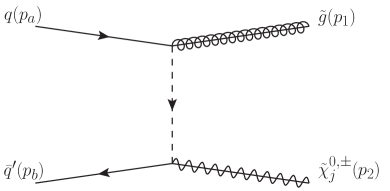
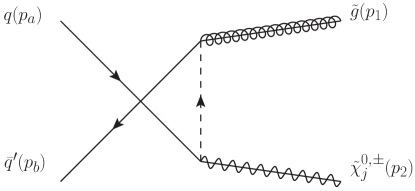
Figure 1: Tree-level $t$- (left) and $u$-channel (right) Feynman diagrams for the associated production of a gluino and a gaugino at hadron colliders. The dashed lines represent squark exchanges.

of a virtual squark $(\tilde{q})$ in the $t$- (left) and $u$-channel (right), where $s=(p_{a}+p_{b})^{2}=(p_{1}+p_{2})^{2}$, $t=(p_{a}-p_{1})^{2}=(p_{b}-p_{2})^{2}$ and $u=(p_{a}-p_{2})^{2}=(p_{b}-p_{1})^{2}$ satisfying $s+t+u=m_{\tilde{g}}^{2}+m_{\tilde{\chi}}^{2}$ are the usual partonic Mandelstam variables. The corresponding squared matrix elements are given by

$$\mathcal{M}_{t}\mathcal{M}^{*}_{t_{c}} = \frac{C_{A}C_{F}\,e\,g_{s}(\mu_{r})}{(m_{\tilde{q}}^{2}-t)(m_{\tilde{q}_{c}}^{2}-t)}(\mathcal{L}^{\prime}\mathcal{L}^{\prime}_{c}+\mathcal{R}^{\prime}\mathcal{R}^{\prime}_{c})(LL_{c}+RR_{c})(m_{\tilde{g}}^{2}-t)(m_{\tilde{\chi}}^{2}-t),$$ (2)

$$\mathcal{M}_{u}\mathcal{M}^{*}_{u_{c}} = \frac{C_{A}C_{F}\,e\,g_{s}(\mu_{r})}{(m_{\tilde{q}}^{2}-u)(m_{\tilde{q}_{c}}^{2}-u)}(\mathcal{L}\mathcal{L}_{c}+\mathcal{R}\mathcal{R}_{c})(L^{\prime}L^{\prime}_{c}+R^{\prime}R^{\prime}_{c})(m_{\tilde{g}}^{2}-u)(m_{\tilde{\chi}}^{2}-u),$$ (3)

$$\mathcal{M}_{t}\mathcal{M}^{*}_{u_{c}} = \frac{C_{A}C_{F}\,e\,g_{s}(\mu_{r})}{(m_{\tilde{q}}^{2}-t)(m_{\tilde{q}_{c}}^{2}-u)}\biggl{[}\left(-s^{2}+t^{2}+u^{2}+(m_{\tilde{\chi}}^{2}+m_{\tilde{g}}^{2})(s-t-u)+2m_{\tilde{g}}^{2}m_{\tilde{\chi}}^{2}\right)$$ (4)

$$\times \left(LL_{c}\mathcal{L}^{\prime}\mathcal{L}^{\prime}_{c}+RR_{c}\mathcal{R}^{\prime}\mathcal{R}^{\prime}_{c}\right)+2m_{\tilde{g}}m_{\tilde{\chi}}s(\mathcal{R}R_{c}\mathcal{L}^{\prime}L^{\prime}_{c}+\mathcal{L}L_{c}\mathcal{R}^{\prime}R^{\prime}_{c})\biggr{]},$$

where the label $c$ of the squark masses $m_{\tilde{q}}$ and couplings $L^{(^{\prime})}$, $R^{(^{\prime})}$, ${\cal L}^{(^{\prime})}$ and ${\cal R}^{(^{\prime})}$ refers to those appearing in the complex conjugate diagrams. Our conventions for the notations of couplings can be found in App. A. The SU(3) colour factors are $C_{A}=3$ and $C_{F}=4/3$. The relation between the electromagnetic and weak couplings $e=g\sin\theta_{W}$ depends on the weak mixing angle $\theta_{W}$, and $g_{s}(\mu_{r})$ is the (renormalisation-scale dependent) strong coupling constant. The total spin- and colour-averaged squared amplitude is then

$$\overline{|{\cal M}|^{2}}=\frac{1}{4C_{A}^{2}}\sum_{\begin{subarray}{c}\tilde{q},\tilde{q}_{c}\end{subarray}}\left(\mathcal{M}_{t}\mathcal{M}^{*}_{t_{c}}+\mathcal{M}_{u}\mathcal{M}^{*}_{u_{c}}-2\operatorname{Re}(\mathcal{M}_{t}\mathcal{M}_{u_{c}}^{*})\right)\,,$$ (5)

where the sum is performed over all squarks in the propagators and where we have inserted a relative minus sign between the $t$- and $u$-channel for the crossing of a fermion line. We have hence generalised the results of the literature Dawson:1983fw ; Baer:1990rq ; Klasen:2006kb ; Beenakker:1996ed ; Berger:1998kh ; Beenakker:1999xh ; Spira:2002rd by allowing for arbitrary squark mixings and mass eigenstates in the squark couplings and propagators, as we have already done in our calculations for slepton Bozzi:2004qq ; Bozzi:2006fw ; Bozzi:2007qr ; Bozzi:2007tea ; Fuks:2013lya and gaugino pair production Debove:2008nr ; Debove:2009ia ; Debove:2010kf ; Debove:2011xj ; Fuks:2012qx ; Fuks:2013vua . This will in particular allow us to extend existing studies of SUSY flavour violation Bozzi:2005sy ; Bozzi:2007me ; delAguila:2008iz ; Fuks:2008ab ; Fuks:2011dg ; DeCausmaecker:2015yca to new processes. Integration over the two-particle phase space dPS${}^{(2)}=\mathrm{d}t/(8\pi s)$ leads to the total partonic cross section

$$\sigma_{ab}(s)=\int\mathrm{d}\sigma_{ab}(s)=\int\frac{1}{2s}\,\overline{|{\cal M|}^{2}}\,{\rm dPS}^{(2)}\,,$$ (6)

and convolution with the factorisation-scale dependent parton distribution functions (PDFs) $f_{a/A}(x_{a},\mu_{f})$ and $f_{b,B}(x_{b},\mu_{f})$

$$\sigma_{AB}~{}=~{}\int M^{2}\frac{\mathrm{d}\sigma_{AB}}{\mathrm{d}M^{2}}(\tau) = \sum_{a,b}\int_{0}^{1}\!\mathrm{d}x_{a}\,\mathrm{d}x_{b}\,\mathrm{d}z[x_{a}f_{a/A}(x_{a},\mu_{f}^{2})][x_{b}f_{b/B}(x_{b},\mu_{f}^{2})]$$ (7)

$$\times \,[z\,\mathrm{d}\sigma_{ab}(z,M^{2},\mu_{r}^{2},\mu_{f}^{2})]\,\delta(\tau-x_{a}x_{b}z)$$

to the total hadronic cross section Collins:1989gx . Here, $\tau=M^{2}/S$ denotes the ratio of the squared invariant mass of the produced SUSY particle pair and the hadronic centre-of-mass energy and is related to the partonic momentum fractions $x_{a}$ and $x_{b}$ by $z=\tau/(x_{a}x_{b})$ with $z=1$ at LO.

For non-mixing squark exchanges, the NLO corrections are well-known Berger:1999mc ; Berger:2000iu ; Berger:2002vd ; Spira:2002rd ; GoncalvesNetto:2012yt . They involve one-loop self-energy, vertex correction and box diagrams interfering with those at tree level as well as squared real gluon and quark emission diagrams, which can involve intermediate on-shell squarks. We have recalculated the full NLO cross section for general squark mixings and mass eigenstates using dimensional regularisation of ultraviolet and infrared divergencies, $\overline{\rm MS}$ renormalisation for couplings and wave functions substituted with a finite shift in the quark-squark-gluino Yukawa coupling to restore SUSY Martin:1993yx , on-shell renormalisation for all squark and gluino masses, and the dipole subtraction method to deal with infrared and collinear divergences Catani:1996jh ; Catani:2002hc . This method exploits the fact that the NLO cross section $\sigma^{(1)}$ can be split into two parts $\sigma^{\{2\}}$ and $\sigma^{\{3\}}$ with two- and three-particle kinematics, respectively, and a collinear counterterm $\sigma^{C}$, that removes initial-state collinear singularities,

$$\sigma^{(1)}=\sigma^{\{3\}}+\sigma^{\{2\}}+\sigma^{C}=\int_{3}[\mathrm{d}\sigma^{R}-\mathrm{d}\sigma^{A}]_{\epsilon=0}+\int_{2}[\mathrm{d}\sigma^{V}+\int_{1}\mathrm{d}\sigma^{A}]_{\epsilon=0}+\sigma^{C}.$$ (8)

The two- and three-particle cross sections are individually regularised by subtracting from the real corrections $\sigma^{R}$ an auxiliary cross section $\sigma^{A}$. The latter captures all infrared-singular behaviour, can be analytically integrated over the singular phase space regions, and is added back to the virtual corrections $\sigma^{A}$. In the limit of mass-degenerate squarks, we achieve full numerical agreement with our previous calculation Berger:1999mc ; Berger:2000iu ; Berger:2002vd , that employed the phase-space slicing method, and the public code Prospino Beenakker:1996ed .

2.2 Refactorisation

Beyond LO, $z=M^{2}/s$ describes the energy fraction going into the hard scattering process. The energy fraction carried by an additional emitted gluon (or quark) is then $1-z$ and describes the distance from partonic threshold. As is well known, large logarithms

$$\left({\alpha_{s}\over 2\pi}\right)^{n}\left[{\ln^{m}(1-z)\over 1-z}\right]_{+}$$ (9)

with $m\leq 2n-1$ remain at higher orders in $\alpha_{s}=g_{s}^{2}/(4\pi)$ even after the cancellation of soft and collinear divergences among the virtual and real emission corrections Kinoshita:1962ur ; Lee:1964is . They arise due to restrictions on the phase space boundary of the latter and spoil the convergence of the perturbative series when $z\rightarrow 1$, i.e. for soft emitted gluons. They must therefore be resummed to all orders in $\alpha_{s}$ for reliable predictions in the threshold region.

Resummation of these logarithmic corrections to all orders and exponentiation can be achieved when the kinematical and dynamical parts of the cross section are fully factorised. By applying a Mellin transform

$$F(N)=\int_{0}^{1}\mathrm{d}y\,y^{N-1}F(y)\,,$$ (10)

to the quantities $F=\sigma_{AB}$, $\sigma_{ab}$, $f_{a/A}$ and $f_{b/B}$ with $y=\tau$, $z$, $x_{a}$ and $x_{b}$ in Eq. (7), the hadronic cross section can be written as a simple product

$$M^{2}\frac{\mathrm{d}\sigma_{AB}}{\mathrm{d}M^{2}}(N-1)=\sum_{a,b}f_{a/A}(N,\mu_{f}^{2})f_{b/B}(N,\mu_{f}^{2})\sigma_{ab}(N,M^{2},\mu_{f}^{2},\mu_{r}^{2})\,.$$ (11)

Large logarithms in $z\rightarrow 1$ then turn into large logarithms of the Mellin variable $N$.

Applying the eikonal Feynman rules, using renormalisation group equation properties and the evolution equations, the partonic cross section can then be refactorised and written in the resummed form Sterman:1986aj ; Kidonakis:1997gm ; Kidonakis:1998bk

$$\begin{split}\sigma^{\rm(res.)}_{ab\rightarrow ij}(N,M^{2},\mu^{2})=&\ \sum_{I}\,\mathcal{H}_{ab\rightarrow ij,I}(M^{2},\mu^{2})\,\Delta_{a}(N,M^{2},\mu^{2})\,\Delta_{b}(N,M^{2},\mu^{2})\\ &\qquad\times\Delta_{ab\rightarrow ij,I}(N,M^{2},\mu^{2})\,,\end{split}$$ (12)

where we have identified the renormalisation and factorisation scales $\mu=\mu_{r}=\mu_{f}$ for brevity. The hard function

$$\mathcal{H}_{ab\rightarrow ij,I}(M^{2},\mu^{2})=\sum_{n=0}^{\infty}a_{s}^{n}(\mu^{2}){\cal H}^{(n)}_{ab\rightarrow ij,I}(M^{2},\mu^{2}),$$ (13)

which is non-singular when $z\rightarrow 1$ or $N\rightarrow\infty$ can be expanded perturbatively in $a_{s}=\alpha_{s}/(2\pi)$ and is discussed in more detail in Sec. 2.3. Like the soft wide-angle function $\Delta_{ab\rightarrow ij,I}$ to be discussed in App. B, it is sensitive to the colour structure of the underlying hard process from which the gluon has been emitted, and can be decomposed into irreducible colour representations $I$. Together with the functions $\Delta_{a,b}$ describing soft collinear radiation, the soft wide-angle function $\Delta_{ab\rightarrow ij,I}$ can be exponentiated in a closed form Vogt:2000ci

$$\Delta_{a}\Delta_{b}\Delta_{ab\rightarrow ij,I}=\exp\Big{[}LG^{(1)}_{ab}(\lambda)+G^{(2)}_{ab\rightarrow ij,I}(\lambda,M^{2}/\mu^{2})+\ldots\Big{]}\,,$$ (14)

with $\lambda=a_{s}\beta_{0}L$, $L=\ln{\bar{N}}$ and ${\bar{N}}=Ne^{\gamma_{E}}$, which contains all the enhanced logarithmic terms. The terms $G^{(1)}_{ab}$ and $G^{(2)}_{ab\rightarrow ij}$ represent the leading-logarithmic (LL) and next-to-leading logarithmic (NLL) approximations Sterman:1986aj ; Kidonakis:1997gm ; Kidonakis:1998bk ; Catani:1989ne ; Catani:1990rp

$$G^{(1)}_{ab}(\lambda) = g_{a}^{(1)}(\lambda)+g_{b}^{(1)}(\lambda),$$ (15)

$$G^{(2)}_{ab\rightarrow ij}(\lambda) = g_{a}^{(2)}(\lambda,M^{2},\mu_{r}^{2},\mu_{f}^{2})+g_{b}^{(2)}(\lambda,M^{2},\mu_{r}^{2},\mu_{f}^{2})+h^{(2)}_{ab\rightarrow ij,I}(\lambda)\,,$$ (16)

with

$$g_{a}^{(1)}(\lambda) = \frac{A_{a}^{(1)}}{2\beta_{0}\lambda}\left[2\lambda+(1-2\lambda)\ln{(1-2\lambda)}\right]\,,$$ (17)

$$g_{a}^{(2)}(\lambda) = \frac{A_{a}^{(1)}\beta_{1}}{2\beta_{0}^{3}}\left[2\lambda+\ln{(1-2\lambda)+\frac{1}{2}\ln^{2}{(1-2\lambda)}}\right]\,,$$ (18)

$$- \frac{A_{a}^{(2)}}{2\beta_{0}^{2}}\left[2\lambda+\ln{(1-2\lambda)}\right]$$

$$+ \frac{A_{a}^{(1)}}{2\beta_{0}}\left[\ln{(1-2\lambda)}\ln{\left(\frac{M^{2}}{\mu_{r}^{2}}\right)}+2\lambda\ln{\left(\frac{\mu_{f}^{2}}{\mu_{r}^{2}}\right)}\right]\,,$$

$$h^{(2)}_{ab\rightarrow ij,I}(\lambda) = \frac{\ln{\left(1-2\lambda\right)}}{2\beta_{0}}D^{(1)}_{ab\rightarrow ij,I}\,,$$ (19)

where the one-loop coefficient $D^{(1)}_{ab\rightarrow ij,I}$ depends on the soft anomalous dimension and is process dependent. While it vanishes for gaugino pair production with coloured particles in the initial state only Debove:2010kf , it must be included for associated gluino-gaugino production, where soft gluons can also be emitted from the final-state gluino. The associated collinear divergence is, however, screened due to the massive emitter. The coefficients in the above equations read

$$A^{(1)}_{a} = 2C_{a}\,,$$ (20)

$$A^{(2)}_{a} = 2C_{a}\left[\left(\frac{67}{18}-\frac{\pi^{2}}{6}\right)C_{A}-\frac{5}{9}n_{f}\right]\,,$$ (21)

$$D^{(1)}_{ab\rightarrow ij,I} = \frac{2\pi}{\alpha_{s}}\operatorname{Re}(\bar{\Gamma}_{ab\rightarrow ij,II})\,,$$ (22)

where $C_{a}=C_{F,A}$ for quarks and gluons and $\bar{\Gamma}_{ab\rightarrow ij,II}$ is the modified diagonal soft anomalous dimension of the colour representation $I$.

2.3 Hard matching coefficient

The resummation of logarithmically enhanced contributions at threshold can be improved by including in the hard function ${\cal H}_{ab\rightarrow ij,I}(M^{2},\mu^{2})$ in Eq. (13) not only the LO cross section

$${\cal H}^{(0)}_{ab\rightarrow ij}(M^{2},\mu^{2})=\sigma^{(0)}_{ab\rightarrow ij}(M^{2}),$$ (23)

but also the $N$-independent contributions of the NLO cross section

$${\cal H}^{(1)}_{ab\rightarrow ij}(M^{2},\mu^{2})=\sigma^{(0)}_{ab\rightarrow ij}(M^{2})\,C^{(1)}_{ab\rightarrow ij}(M^{2},\mu^{2}),$$ (24)

which beyond NLO are multiplied by threshold logarithms. The hard matching coefficient $C^{(1)}_{ab\rightarrow ij}(M^{2},\mu^{2})$ is obtained by computing the Mellin transform of the full NLO corrections $\sigma^{(1)}_{ab\rightarrow ij}(M^{2},\mu^{2})/\sigma^{(0)}_{ab\rightarrow ij}(M^{2})$ described in Sec. 2.1, keeping only the $N$-independent terms. In the case of associated gluino-gaugino production, this is again simplified by the fact that there is only one colour basis tensor, so that the index $I$ can be dropped.

In Eq. (8), the three-particle contributions to $\sigma^{(1)}$ can safely be neglected, since all infrared divergences are canceled after subtracting from $\mathrm{d}\sigma^{R}$ the auxiliary cross section $\mathrm{d}\sigma^{A}$ and the finite terms are phase-space suppressed near threshold Beenakker:2011sf ; Beenakker:2013mva . The virtual corrections $\mathrm{d}\sigma^{V}$ and the integrated dipoles $\int_{1}\mathrm{d}\sigma^{A}$ are straightforward to transform into Mellin space in the invariant-mass threshold approach, since they are proportional to $\delta(1-z)$ and thus constant in $N$. The corresponding analytical results can be found in Refs. Berger:2000iu and Catani:1996jh ; Catani:2002hc , respectively. The collinear remainder $\sigma^{C}$ is usually split into contributions from two insertion operators $P$ and $K$ Catani:2002hc

$$\sigma^{C}=\sum_{a^{\prime}}\int_{0}^{1}\mathrm{d}x\int_{2}[\mathrm{d}\sigma^{(0)}_{a^{\prime}b}(xp_{a},p_{b})\otimes\langle a^{\prime}|{\mbox{\boldmath$P$}}+{\mbox{\boldmath$K$}}|a\rangle(x)+(a\leftrightarrow b)]_{\epsilon=0}.$$ (25)

The former is directly related to the regularised Altarelli-Parisi splitting distributions at ${\cal O}(\alpha_{s})$, while the latter depends on the factorisation scheme and on the regular parts of the Altarelli-Parisi splitting distributions. For the initial quark $a$, we obtain after transforming to Mellin space

$$\langle{\mbox{\boldmath$P$}}(N)\rangle=\frac{\alpha_{s}}{2\pi}\biggl{[}(2C_{F}-C_{A})\ln\frac{\mu_{f}^{2}}{s}+C_{A}\ln\frac{\mu_{f}^{2}}{m_{\tilde{g}}^{2}-t}\biggl{]}\biggl{[}\ln{\bar{N}}-{3\over 4}\biggl{]}\,+\,\mathcal{O}\left(\frac{1}{N}\right)$$ (26)

and

$$\langle{\mbox{\boldmath$K$}}(N)\rangle = \frac{\alpha_{s}}{2\pi}\Bigg{\{}2C_{F}\ln^{2}{\bar{N}}+C_{A}\left[\ln{m_{\tilde{g}}^{2}\over m_{\tilde{g}}^{2}-t}+1\right]\ln{\bar{N}}+{\pi^{2}\over 2}C_{F}-\gamma_{q}-K_{q}$$

$$+ {C_{A}\over 4}\biggl{[}1+4\,{\rm Li}_{2}{2m_{\tilde{g}}^{2}-t\over m_{\tilde{g}}^{2}}+\bigg{(}1+4\ln{m_{\tilde{g}}^{2}\over m_{\tilde{g}}^{2}-t}+2{m_{\tilde{g}}^{2}\over m_{\tilde{g}}^{2}-t}\bigg{)}\ln{m_{\tilde{g}}^{2}\over 2m_{\tilde{g}}^{2}-t}$$

$$\ +3\ln\bigg{(}1+{2m_{\tilde{g}}\over m_{\tilde{g}}^{2}-t}\left(m_{\tilde{g}}-\sqrt{2m_{\tilde{g}}^{2}-t}\ \right)\bigg{)}+6{m_{\tilde{g}}\over m_{\tilde{g}}+\sqrt{2m_{\tilde{g}}^{2}-t}}-3\biggl{]}\Bigg{\}}+\mathcal{O}\left(\frac{1}{N}\right)$$

with

$$\gamma_{q}~{}=~{}{3\over 2}\,C_{F} \ ,\ K_{q}~{}=~{}\left({7\over 2}-{\pi^{2}\over 6}\right)\,C_{F}\,,$$ (28)

and similarly for the incoming antiquark $b$ with $t\rightarrow u$. Non-diagonal operators give only $1/N$-suppressed contributions, and there are no initial-state gluons at LO. In the limit of $C_{A}\rightarrow 0$, one recovers the well-known results for Drell-Yan like processes Debove:2010kf .

For the hard matching coefficient, only the $N$-independent parts of the above results are needed. The logarithmic terms terms can be used to check the resummed cross section when re-expanded to NLO (see below). Since the $1/N$ terms have been systematically neglected, the collinear improvement of the resummation formalism suggested in Refs. Kramer:1996iq ; Catani:2001ic has not been performed in contrast to our calculations for uncoloured slepton Bozzi:2007qr and gaugino pair production Debove:2010kf , but similarly to the calculations for coloured squarks and gluinos Beenakker:2009ha ; Beenakker:2011sf ; Beenakker:2013mva . This is in particular due to the fact that analytic results for the subleading terms in the Mellin transform of the collinear remainder can not be obtained. For the Drell-Yan process, the constant terms in the hard function ${\cal H}_{ab\rightarrow ij}^{(1)}(M^{2},\mu^{2})$ are sometimes also exponentiated based on the argument that they factorise the complete Born cross section, include finite remainders of the infrared singularities in the virtual corrections and are thus related to the corresponding singularities in the real corrections giving rise to the large logarithms Eynck:2003fn . However, similarly to gaugino pair production Debove:2010kf , gluino-gaugino associated production does not proceed through a single $s$-channel diagram (see Fig. 1) and the virtual corrections factorise only at the level of amplitudes, and not at the level of the full cross section Berger:1999mc ; Berger:2000iu ; Berger:2002vd . Resumming these finite terms is therefore not justified in this case.

2.4 Matching and inverse Mellin transform

While near threshold the resummed cross section is a valid approximation, far from it the normal perturbative calculation should be used. A reliable prediction in all kinematic regions is then obtained through a consistent matching of the two results with

$$\sigma_{ab}=\sigma_{ab}^{\rm(res.)}+\sigma_{ab}^{\rm(f.o.)}-\sigma_{ab}^{\rm(exp.)}\,.$$ (29)

Here, the resummed cross section $\sigma_{ab}^{\rm(res.)}$ in Eq. (12) has been re-expanded to NLO, yielding $\sigma_{ab}^{\rm(exp.)}$, and subtracted from the fixed-order calculation $\sigma_{ab}^{\rm(f.o.)}$ in Eq. (8) in order to avoid the double counting of the logarithmically enhanced contributions. At ${\cal O}(\alpha_{s})$, we then obtain

$$\sigma_{ab}^{\rm(exp.)} = \mathcal{H}^{(0)}_{ab\rightarrow ij,I}(M^{2},\mu^{2})+\frac{\alpha_{s}}{2\pi}\mathcal{H}^{(1)}_{ab\rightarrow ij,I}(M^{2},\mu^{2})+\frac{\alpha_{s}}{2\pi}\,\mathcal{H}^{(0)}_{ab\rightarrow ij,I}(M^{2},\mu^{2})$$ (30)

$$\times \left[(A_{a}^{(1)}+A_{b}^{(1)})\ln^{2}{\bar{N}}+\left((A_{a}^{(1)}+A_{b}^{(1)})\ln{\frac{\mu_{f}^{2}}{s}}-2D^{(1)}_{ab\rightarrow ij,I}\right)\ln{\bar{N}}\right]\,,$$

where $\mathcal{H}^{(0)}$ and $\mathcal{H}^{(1)}$ are the first and second order parts of the hard matching coefficient (see Sec. 2.3).

Inserting $A_{a}^{(1)}=A_{b}^{(1)}=2C_{F}$ (cf. Eq. (20)), the leading logarithms $\alpha_{s}/(2\pi)\ln^{2}{\bar{N}}$ have the coefficient $4C_{F}$, which agrees with the leading logarithmic contribution to the hard matching coefficient arising exclusively from the $K$-operators in the collinear remainder in Eq (2.3). The coefficient $4C_{F}$ also governs the scale- and more precisely the $\ln(\mu_{f}^{2}/s)$-dependent part of the next-to-leading logarithms $\alpha_{s}/(2\pi)\ln{\bar{N}}$, which agrees with the corresponding parts of the quark and antiquark $P$-operator expectation values in the collinear remainder in Eq. (26). In contrast, the $C_{A}$-terms depending on $\mu_{f}$ cancel there, while the remaining NLL terms are

$$C_{A}\left[\ln{\frac{s}{m_{\tilde{g}}^{2}-t}}+\ln{\frac{s}{m_{\tilde{g}}^{2}-u}}\right]\,.$$ (31)

From the $K$-operators in Eq. (2.3), we get in addition the NLL contributions

$$C_{A}\left[\ln\frac{m_{\tilde{g}}^{2}}{m_{\tilde{g}}^{2}-t}+\ln{\frac{m_{\tilde{g}}^{2}}{m_{\tilde{g}}^{2}-u}}+2\right]\,,$$ (32)

which together correctly reproduce the contribution from the soft anomalous dimension in Eq. (54) and Eq.(30).

Having computed the resummed and the perturbatively expanded results in Mellin space, we must multiply them with the $N$-moments of the PDFs according to Eq. (11) and perform an inverse Mellin transform

$$M^{2}{{\rm d}\sigma_{AB}\over{\rm d}M^{2}}(\tau) = {1\over 2\pi i}\int_{{\cal C}_{N}}{\rm d}N\tau^{-N}M^{2}{{\rm d}\sigma_{AB}(N)\over{\rm d}M^{2}}$$ (33)

in order to obtain the hadronic cross section as a function of $\tau=M^{2}/S$. Special attention must be paid to the singularities in the resummed exponents $G_{ab}^{(1,2)}$, which are situated at $\lambda=1/2$ and are related to the Landau pole of the perturbative coupling $a_{s}$. To avoid this pole as well as those in the Mellin moments of the PDFs related to the small-$x$ (Regge) singularity $f_{a/A}(x,\mu_{0}^{2})\propto x^{\alpha}(1-x)^{\beta}$ with $\alpha<0$, we choose an integration contour ${\cal C}_{N}$ according to the principal value procedure proposed in Ref. Contopanagos:1993yq and the minimal prescription proposed in Ref. Catani:1996yz . We define two branches

$${\cal C}_{N}:~{}~{}N=C+ze^{\pm i\phi}~{}~{}{\rm with}~{}~{}z\in[0,\infty[,$$ (34)

where the constant $C$ is chosen such that the singularities of the $N$-moments of the PDFs lie to the left and the Landau pole to the right of the integration contour. Formally the angle $\phi$ can be chosen in the range $[\pi/2,\pi[$, but the integral converges faster if $\phi>\pi/2$.

The Mellin moments of the PDFs are obtained by fitting to the parameterisations tabulated in $x$-space the functional form used by the MSTW collaboration Martin:2009iq

$$f(x)=A_{0}\,x^{A_{1}}\,(1-x)^{A_{2}}\,\left(1+A_{3}\,\sqrt{x}+A_{4}\,x+A_{5}\,x^{\frac{3}{2}}\right)+A_{6}\,x^{2}+A_{7}\,x^{\frac{5}{2}}\,,$$ (35)

which has the advantage that it can be transformed analytically with the result

$$F(x) = A_{0}\,\Gamma\left(y\right)\,\mathrm{B^{\prime}}\left(A_{1}+N,y\right)+A_{3}\,\mathrm{B^{\prime}}\left(A_{1}+N+\frac{1}{2},y\right)+A_{4}\mathrm{B^{\prime}}\left(A_{1}+N+1,y\right)$$ (36)

$$+ A_{5}\mathrm{B^{\prime}}\left(A_{1}+N+\frac{3}{2},y\right)+A_{6}\mathrm{B^{\prime}}\left(A_{1}+N+2,y\right)+A_{7}\mathrm{B^{\prime}}\left(A_{1}+N+\frac{5}{2},y\right)\,.$$

Here, $y=A_{2}+1$ and $\mathrm{B^{\prime}}(x,y)=\mathrm{B}(x,y)/\Gamma(y)=\Gamma(x)/\Gamma(x+y)$. We have verified that we obtain good fits not only for the MMHT2014NLO118 Martin:2009iq , but also for the CT14NLO fits Dulat:2015mca up to large values of $x$ and for all typical factorisation scales, even though the latter are obtained with an ansatz including an exponential function. The fit to the NNPDF$\_$30$\_$nlo$\_$as$\_$0118 PDFs Ball:2014uwa is slightly less stable in the large-$x$ region. They will therefore only be used for estimates of the PDF uncertainty. We compute in this case first an (approximately PDF-independent) $K$-factor, i.e. the ratio of NLL+NLO over NLO cross sections, using stable (e.g. CT14NLO) PDFs and then multiply with it the NLO calculation convoluted with NNPDFs directly in $x$ space.

3 Numerical results

We now turn to our numerical results. For our calculations, we have used the Particle Data Group (PDG) values for the Standard Model parameters, in particular for the value of the strong coupling constant at the $Z$-pole $\alpha_{s}(M_{Z})$ Agashe:2014kda . In our LO and NLO/NLL+NLO calculations, it is evaluated in the one- and two-loop approximations, respectively, with five active quark flavours. All light quarks including the bottom quark are taken as massless. The top quark is decoupled. Its (pole) mass enters only in the gluino self-energy and has little numerical influence on the production cross sections.

3.1 Benchmark scenario

Our results are given for a specific phenomenological MSSM (pMSSM) benchmark scenario with 13 free parameters. These parameters are listed together with the corresponding fitted numerical values in Tab. 1.

$\tan\beta$	$\mu$	$m_{A}$	$M_{1}$	$M_{3}$	$M_{Q_{1,2}}$	$M_{Q_{3}}$	$M_{U_{1,2}}$	$M_{U_{3}}$	$M_{D_{12}}$	$M_{D_{3}}$	$M_{L}$	$A_{f}$
21	​​​773​​​	1300	​​315	​​1892	​​2288	​​425	​​1758	​​2754	​​552	​​714	​​1553	​​-2200

Table 1: Higgs sector and soft SUSY breaking parameters in our pMSSM-13 benchmark model. All values except the one for $\tan\beta$ are in GeV.

Our scenario is inspired by the benchmark point II of Ref. DeCausmaecker:2015yca , that has been obtained with a Markov Chain Monte Carlo (MCMC) scan using also PDG values for the Standard Model parameters. This 19-parameter scan has been performed with a focus on non-minimal flavour violation (NMFV). It therefore included seven flavour-violation parameters and checked in particular the most stringent flavour-changing neutral current (FCNC) constraints from rare $B$- and $K$-decays. Since we are not interested in NMFV, we set these parameters all to zero. This reduces the SUSY contributions to the rare meson decays. To compensate for the reduced mass splitting in the top squark sector and obtain a Higgs-boson mass compatible with the measured value, we have instead changed the sign and increased the absolute value of the trilinear coupling $A_{f}$. We then still obtain a neutralino lightest SUSY particle and in addition a light top squark, which leads to a viable dark matter candidate and allows in general for sufficient stop coannihilation to reproduce the observed dark matter relic density Klasen:2015uma ; Harz:2012fz ; Harz:2014tma ; Harz:2014gaa ; Harz:2016dql . While we continue to impose the GUT relation between the bino and wino mass parameters, $M_{1}\simeq M_{2}/2$, we allow the gluino mass parameter $M_{3}$ to vary independently, which brings us to $19-7+1=13$ free parameters. For our default scenario, we still impose the GUT relation for $M_{3}\simeq 6M_{1}$.

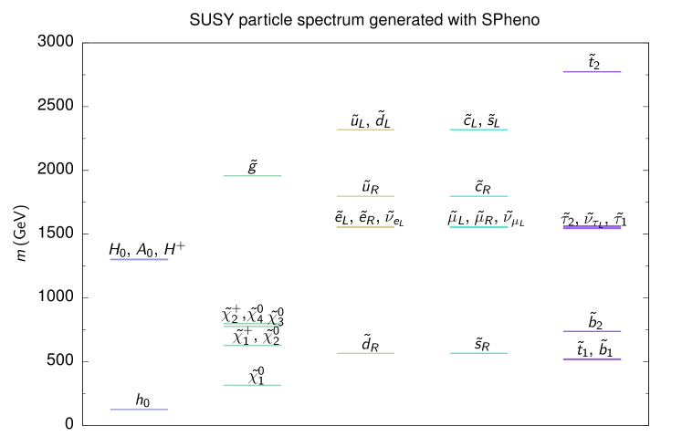
Figure 2: Visualised mass spectrum for the benchmark point defined in Tab. 1. Particles are grouped in Higgs particles, gauginos, first-, second- and third-generation sfermions (left to right).

The physical SUSY mass spectrum is obtained with SPheno 3.37 Porod:2011nf and shown schematically in Fig. 2. Apart from the FCNC, the Higgs-boson and neutralino dark matter data, also the observed value of the anomalous magnetic moment of the muon, which is unaffected by the gluino mass, is reproduced in this scenario. In addition, it satisfies the increasingly stringent constraints that are imposed on the masses of the SUSY particles from direct search results at the LHC. For example, with the 2015 data from Run II, ATLAS and CMS exclude gluino masses up to 1400 and 1280 GeV, assuming masses of the lightest neutralino of up to 600 and 800 GeV, respectively Aad:2016jxj ; CMS:2015vqc . Mass-degenerate light charginos and second-lightest neutralinos produced electroweakly have been excluded at Run I up to 465 and 720 GeV in the case of massless lightest neutralinos Aad:2014vma ; Khachatryan:2014qwa . These exclusion limits are however not valid within the general pMSSM, as they have been obtained assuming direct production cross sections and simplified decay scenarios.

As we have already mentioned in the previous section, our calculations allow for arbitrary squark mixings and mass eigenstates in the appearing couplings and propagators. The mixing of squark interaction eigenstates is numerically relevant only for third-generation (and in particular top) squarks. Since the top and bottom quark PDFs are small, the mixing influences predominantly the gluino self-energy diagram with little (below the percent level) numerical effect. In contrast, the masses of first- and second generation squarks in our scenario span a large range from about 600 to 2300 GeV. Averaging over these masses leads to cross sections that are almost a factor of two larger. This is already true at LO, since the dominant effect comes from squark propagators already present there. If the LO calculations are performed without averaging and corrected by a mass-averaged $K$-factor, as it is, e.g., done in Prospino Beenakker:1996ed , differences of about 5% remain. These differences originate in particular from intermediate squarks at NLO, which in the general case can sometimes be on-shell, while they cannot be on-shell in the mass-averaged case.

3.2 Invariant mass distribution

The associated production of a gluino and the lightest neutralino will be difficult to observe at the LHC, as the latter escapes directly undetected. It is therefore more promising to study the associated production of a gluino with the second-lightest neutralino (or the lightest chargino of often equal mass), since it will decay into an additional $Z$ (or $W$) boson, whose leptonic decay products will then lead to an identifiable signal and better background suppression. As our default PDFs, we use CT14NLO at NLO and NLL+NLO and CT14LL together with the one-loop approximation for $\alpha_{s}$ at LO (see above) Dulat:2015mca .

In the upper panel of Fig. 3, we show the invariant-mass distribution given by Eq. (33), for

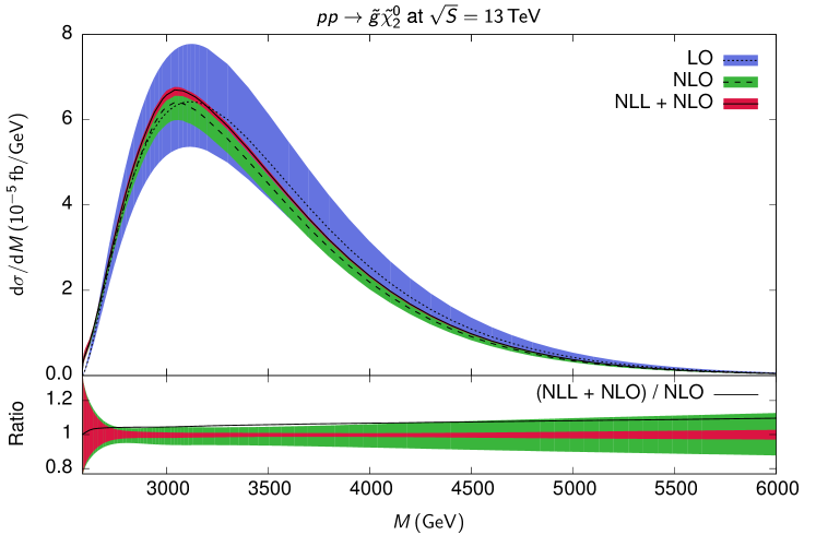
Figure 3: Upper panel: Invariant mass distribution for the process $pp\rightarrow\tilde{g}\tilde{\chi}_{2}^{0}$ at the LHC with a centre-of-mass energy of $\sqrt{S}=13$ TeV at the LO (blue), NLO (green) and NLL+NLO (red) accuracy. Lower panel: Corresponding relative scale uncertainties and the NLL+NLO/NLO $K$-factor (black line).

the production of a gluino with a mass of 1892 GeV and a second-lightest neutralino with a mass of 630 GeV, where both masses have been chosen such that they lie beyond current LHC limits even in simplified scenarios. The cross sections peak at about 3.2 TeV and then fall off towards higher invariant masses $M$. Due to additional radiation, the maximum is shifted from LO (blue) to NLO (green) and NLL+NLO (red) towards slightly smaller values of $M$. At the same time, the scale uncertainties (shaded bands) are significantly reduced from LO to NLO and then again to NLL+NLO. The second reduction is more clearly visible in the lower panel of Fig. 3, where it amounts to a change from $\pm 12\%$ to $\pm 3\%$ at high invariant masses. The scale errors have been obtained here in the usual way from individual variations of the factorisation and renormalisation scales by a factor of two about the average mass of the two produced final-state particles, $(m_{\tilde{g}}+m_{\tilde{\chi}_{2}^{0}})/2$, excluding relative factors of four. In the high-mass region, the corrections from threshold resummation at NLL increase the central NLO cross section by up to 10% (black line) and more closer to the threshold.

3.3 Scale uncertainty of the total cross section

After integrating over the invariant mass $M$ in Eq. (33), we obtain the total production cross section for a gluino and a second-lightest neutralino. For a process that depends already at LO on the strong coupling constant, one expects the significant (approximately logarithmic) scale dependence to be already reduced at NLO. This is clearly visible in Fig. 4, where the NLO result (green dashed curve) shows the characteristic maximum at approximately half the central renormalisation and factorisation scale (upper panel). The scale dependence is further reduced at NLL+NLO (red full curve), as it was already the case for the invariant-mass distribution (see above). When the NLL+NLO result is re-expanded to NLO (blue dotted curve), it becomes a good approximation to the full NLO result in particular for large scale choices, when the logarithmic terms dominate the cross section. This is also true when the renormalisation (central panel) and factorisation scales (lower panel) are varied individually and not together. The lower two panels also demonstrate nicely the interplay of the renormalisation and factorisation scale behaviour in the NLO and NLL+NLO cross sections, that together produce the stabilised behaviour in the upper panel with a large plateau in particular at NLL+NLO. We have verified that we obtain similar results also for larger gluino masses of, e.g., 3 TeV.

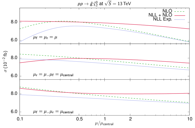
Figure 4: Total cross section for the process $pp\rightarrow\tilde{g}\tilde{\chi}_{2}^{0}$ at the LHC with a centre-of-mass energy of $\sqrt{S}=13$ TeV at NLO (green dashed curve), NLL+NLO (red full curve) and after the re-expansion of the NLL result to NLO (blue dotted curve). We vary the renormalisation scale and factorisation scale together (upper panel), only the renormalisation scale with fixed factorisation scale (central panel) and vice versa (lower panel).

3.4 Gluino mass dependence of the total cross section

Since the gluino mass is unknown, it is interesting to compute the total cross section for associated gluino-neutralino production as a function of the gluino or gaugino mass. The gluino mass dependence is shown in the upper panel of Fig. 5 and in tabular form in Tab. 2 in App. C. As expected, the cross section falls steeply with the gluino mass from 3 to 0.01 fb in the range $m_{\tilde{g}}\in[500,3000]$ GeV. With LHC luminosities of currently a few fb^-1 and in the near future a few 100 fb^-1 at $\sqrt{S}=13$ TeV, these cross sections will soon be observable. In the high-luminosity phase of the LHC, expected to collect up to 3000 fb^-1, even larger gluino masses can be reached that may kinematically no longer be accessible in the strong production of gluino pairs.

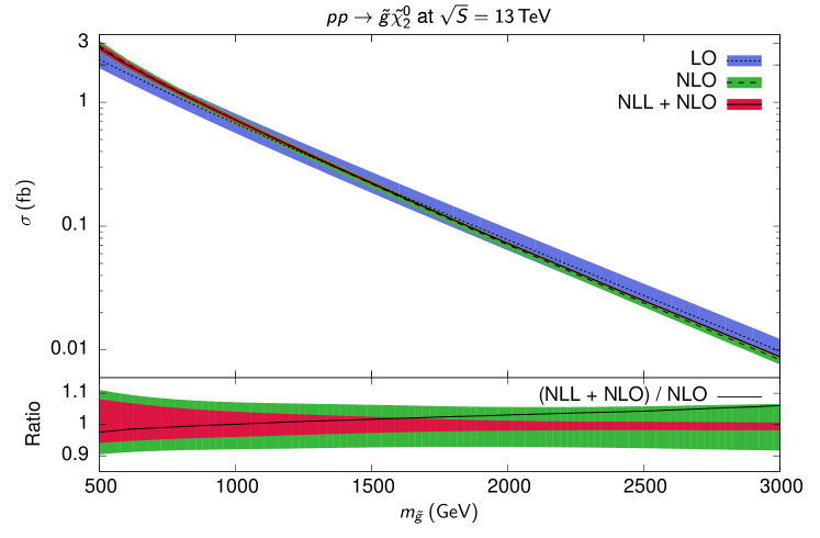
Figure 5: Upper panel: Total cross section for the process $pp\rightarrow\tilde{g}\tilde{\chi}_{2}^{0}$ at the LHC with a centre-of-mass energy of $\sqrt{S}=13$ TeV in LO (blue), NLO (green) and NLL+NLO (red) as a function of the gluino mass. Lower panel: Corresponding relative scale uncertainties and the NLL+NLO/NLO $K$-factor (black line).

As the lower panel of Fig. 5 shows, the NLO scale uncertainty on the total cross section of $\pm 10$% at 500 GeV decreases only slightly towards higher gluino masses. This is in sharp contrast to the NLL+NLO prediction, that has already a smaller scale error of $\pm 7$% at 500 GeV and that becomes much more reliable with an error of only a few percent at large gluino masses. At the same time, the NLO cross section is increased at NLL+NLO by 7 (black line) to 20% for gluino masses of 3 to 6 TeV, respectively.

3.5 Gaugino mass dependence of the total cross section

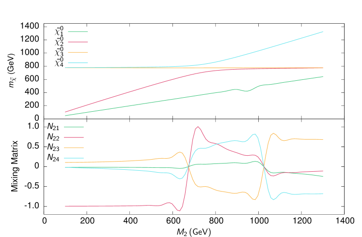
Figure 6: Dependence of the neutralino mass eigenvalues (upper panel) and mixing matrix elements of the second-lightest neutralino (lower panel) on the wino and bino mass parameters $M_{2}\simeq 2\,M_{1}$. All other Higgs and soft SUSY-breaking parameters have been kept fixed and set to the values of our benchmark scenario.

Similarly to the gluino mass dependence, the total cross section for gluino-gaugino associated production decreases with the gaugino mass. Since the mass of the second-lightest neutralino (and the almost identical one of the lightest chargino) is a dependent physical mass obtained after diagonalisation of the neutralino (or chargino) mass matrix with the mixing matrix $N$, we vary instead the bino mass parameter $M_{1}$, which fixes immediately also the wino mass parameter $M_{2}$ through the GUT relation $M_{2}\simeq 2\,M_{1}$. As one can see in the upper panel of Fig. 6, the mass eigenvalue of the second-lightest neutralino $\tilde{\chi}_{2}^{0}$ increases linearly with $M_{2}$ up to $M_{2}=\mu=773$ GeV, where a typical avoided crossing occurs. At higher values of $M_{2}$, it is the mass eigenvalue of $\tilde{\chi}_{4}^{0}$ that depends linearly on $M_{2}$, while the mass of $\tilde{\chi}_{2}^{0}$ stays constant. Accordingly, the decomposition of $\tilde{\chi}_{2}^{0}$ changes from wino-type (large mixing matrix element $N_{22}$, red curve) to higgsino-type (large mixing matrix elements $N_{23}$ and $N_{24}$, yellow and blue curves). Both features will of course influence the production cross section of the process $pp\rightarrow\tilde{g}\tilde{\chi}_{2}^{0}$.

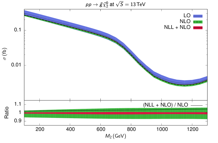
Figure 7: Upper panel: Total cross section for the process $pp\rightarrow\tilde{g}\tilde{\chi}_{2}^{0}$ at the LHC with a centre-of-mass energy of $\sqrt{S}=13$ TeV in LO (blue), NLO (green) and NLL+NLO (red) as a function of the wino mass parameter $M_{2}$. The bino mass parameter has been varied simultaneously using the GUT relation $M_{1}\simeq M_{2}/2$. Lower panel: Corresponding relative scale uncertainties and the NLL+NLO/NLO $K$-factor (black line).

The dependence of the cross section on the wino mass parameter is shown in Fig. 7 and in tabular form in Tab. 3 in App. C. As expected, it falls with $M_{2}$ as long as the physical mass of $\tilde{\chi}_{2}^{0}$ changes. For $M_{2}>\mu$, the neutralino becomes higgsino-like and couples mostly via quark Yukawa couplings. Since the heavy quark PDFs in the proton are small, the cross section starts to fall even faster than before despite the fact that the gaugino mass remains constant and the available phase space no longer changes. Interestingly, the cross section increases again somewhat for $M_{2}>1150$ GeV, which can be explained with a slightly increasing bino component (see Fig. 6). The scale uncertainty (shaded bands) is drastically reduced from LO (blue) to NLO (green), in particular at low values of $M_{2}$. However, the NLO scale dependence increases with $M_{2}$ up to $M_{2}=\mu=773$ GeV due to the rising contribution of the large logarithms. This can be seen more clearly in the lower panel of Fig. 7. Beyond this mass, the scale dependence remains constant as expected. A similar trend is observed in the NLL+NLO scale dependence (red), albeit at an again much lower level. To be specific, it rises only from $\pm 1$ to $\pm 3$% compared to a scale dependence at NLO that rises from $\pm 3$ to $\pm 6$%. The $K$-factor (black line) increases also with $M_{2}$ from 1.02 to 1.07.

3.6 Parton density uncertainty of the total cross section

While the scale uncertainty is expected to be reduced due to the resummation of large logarithms, the PDF uncertainty is normally not improved by this procedure. It is usually estimated by propagating the experimental uncertainties on the fitted data points through to the PDFs (e.g. linearly via a Hessian method) and leads to the production of orthogonal eigenvector PDF sets corresponding to a 90% confidence level. This method is employed by the CTEQ and MMHT collaborations and has been found to produce comparable results to the more intricate Lagrange multiplier method Dulat:2015mca ; Martin:2009iq . The uncertainty on the cross section is then obtained from

$$\Delta\sigma_{\rm PDF+} = \sqrt{\sum_{i=1}^{n}\left[\max\left(\sigma_{+i}-\sigma_{0},\sigma_{-i}-\sigma_{0},0\right)\right]^{2}},$$ (37)

$$\Delta\sigma_{\rm PDF-} = \sqrt{\sum_{i=1}^{n}\left[\max\left(\sigma_{0}-\sigma_{+i},\sigma_{0}-\sigma_{-i},0\right)\right]^{2}},$$ (38)

where $n=28$ and 25 is the number of eigenvector directions in the CT14 and MMHT2014 fits, respectively. Since the MMHT PDF sets are only available for 68% and not 90% confidence level, the corresponding error must be multiplied by the standard factor of 1.645 for compatibility. The NNPDF collaboration uses instead a Monte Carlo method, where the PDF uncertainty is obtained by sampling the available replicas Ball:2014uwa . Since PDF uncertainties are usually not produced for LO fits and since the results are very similar at NLO and NLL+NLO, we will only study them at the level of NLL+NLO cross sections. For NNPDF, we estimate the PDF uncertainty using the $K$-factor method described in Sec. 2.4.

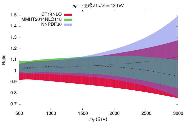
Figure 8: Relative PDF uncertainties of the total cross section for the process $pp\rightarrow\tilde{g}\tilde{\chi}_{2}^{0}$ at the LHC with a centre-of-mass energy of $\sqrt{S}=13$ TeV in NLL+NLO. The uncertainties are shown for three different PDFs, CT14NLO (red), MMHT2014NLO118 (green) and NNPDF30 (blue), as a function of the gluino mass $m_{\tilde{g}}$.

The results are shown in Fig. 8. As one can see, the estimates by the three groups overlap to a large extent. While the three individual PDF uncertainties are still relatively small and comparable to the scale uncertainty with about $\pm 5$% at small values of the gluino mass of about 500 GeV (cf. Fig. 5), they increase rather than decrease with $m_{\tilde{g}}$ and reach a level of $\pm 20$% at 3 TeV. This is of course due the fact that the PDFs are much less constrained at large than at intermediate values of the parton momentum fraction $x$. Compared to the central prediction with CT14, those with MMHT2014 and NNPDF30 lie systematically higher by a few percent. The increase of the uncertainty towards larger $x$ is less pronounced in MMHT and more pronounced in NNPDF. It will therefore be interesting to study the impact of threshold-improved PDFs in future work, as it was done for squark and gluino production Bonvini:2015ira ; Beenakker:2015rna . It is important to note that the scale uncertaintites computed in the previous sections and the PDF uncertainty computed in this section are independent and therefore usually added in quadrature for a reliable estimate of the total theoretical uncertainty.

4 Conclusion

We have presented in this paper a threshold resummation calculation at the NLL+NLO accuracy for the associated production of gluinos and gauginos at the LHC. This process is of intermediate strength compared to the strong production of gluino (and squark) pairs and the electroweak production of gaugino (and slepton) pairs. It can in particular become relevant should the gluinos prove to be too heavy to be pair-produced at the LHC. This situation would not be unexpected, if one takes the GUT relation between the gaugino masses seriously, which predicts $M_{1}=M_{2}/2=M_{3}/6$ after renormalisation group running at the weak scale. Lighter gluinos, e.g. with a possible cosmological impact through their coannihilation with gauginos, typically require non-minimal assumptions such as non-universal gaugino masses or vector-like supermultiplets Profumo:2004wk ; Nagata:2015hha ; Ellis:2015vna ; Nath:2016kfp . Conversely, associated gluino-gaugino production could also become phenomenologically important in the less likely case that the gauginos lie beyond the kinematic reach of the LHC, so that e.g. the gravitino becomes the lightest SUSY particle and its associated production with (relatively light) gluinos an interesting search channel Klasen:2006kb .

Our investigations required the (re-)calculation of the full NLO corrections, which we generalised to the case of non-degenerate squark masses, and of the process-dependent soft anomalous dimension and hard matching coefficients, which we could show to be consistent with each other. For a typical benchmark scenario, obtained in a recent MCMC fit of the Higgs boson, FCNC, muon magnetic moment and LHC data, we presented numerical predictions for the invariant-mass distribution and the total cross section as a function of the gluino or gaugino mass. The resummation of the NLL contributions increased the NLO cross sections at large invariant mass by up to 10% and stabilised them dramatically with respect to the scale dependence. As expected, the PDF uncertainty was, however, not reduced. It will therefore be interesting to study the impact of threshold-improved PDFs in the future.

Numerical predictions for other SUSY scenarios are available from the authors upon request. The calculation will also be included in the next release of the public code Resummino Fuks:2013vua . Its application to the associated production of gluinos and gravitinos would not only require the inclusion of the additional $s$-channel gluon exchange, but also a full NLL+NLO calculation for the gluon-initiated diagrams. The NLL+NLO calculation for the associated production of squarks and gauginos is in progress and will be presented elsewhere.

Appendix A Coupling conventions

The conventions for the couplings appearing in our calculations are defined in Fig. 9. The electromagnetic and (renormalisation scale dependent) strong coupling constants are denoted by $e$ and $g_{s}(\mu_{r})$, respectively. $T^{a}_{\beta\alpha}$ and $f_{abc}$ are SU(3) colour matrices in the fundamental representation and structure constants, $\gamma^{\mu}$ and $P_{L,R}$ Dirac matrices and chirality projection operators. The latter are associated with generic MSSM coupling constants $L^{(^{\prime})}$, $R^{(^{\prime})}$, ${\cal L}^{(^{\prime})}$ and ${\cal R}^{(^{\prime})}$ which involve squark and gaugino mixing matrices and can be found together with the quartic squark couplings $X$ and $Y$ in Refs. Haber:1984rc ; Gunion:1984yn .

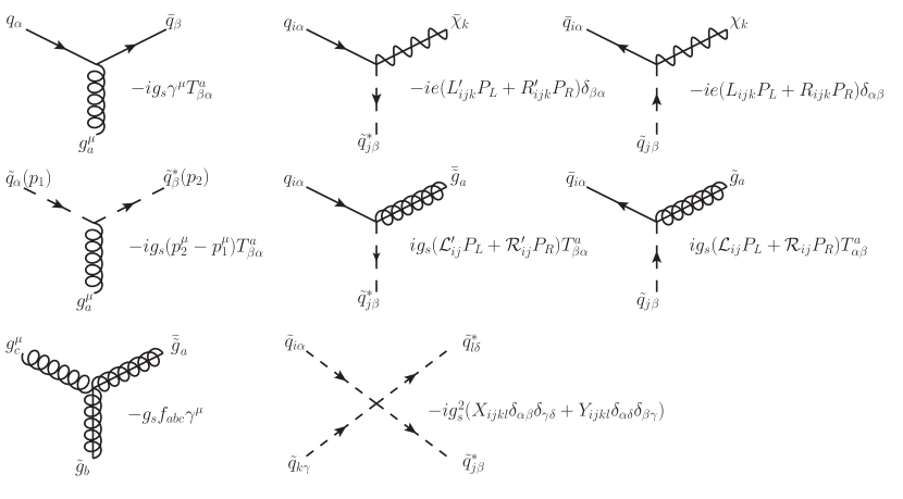
Figure 9: Interaction vertices appearing in the associated production of gluinos and gauginos at LO and NLO. All momenta are ingoing, and arrows describe charge/fermion flow.

Appendix B Soft anomalous dimension

If the calculation of the (modified) soft anomalous dimension is performed in the axial gauge with a gauge vector $n^{\mu}$, it is given by

$${\bar{\Gamma}}_{ab\rightarrow ij,IJ}=\Gamma_{ab\rightarrow ij,IJ}-\frac{\alpha_{s}}{2\pi}\sum\limits_{k={\{a,b\}}}C_{k}\left(1-\ln{\left(2\frac{(v_{k}\cdot n)^{2}}{|n|^{2}}\right)}-i\pi\right)\delta_{IJ},$$ (39)

where one sums over the two incoming particles and where $|n|^{2}=-n^{2}-i\epsilon$ Kidonakis:1997gm ; Beenakker:2009ha . The dimensionless vector $v_{k}$ is given by the momentum of the incoming massless particle $k$ rescaled by $\sqrt{2/s}$. Here, the soft anomalous dimension has been modified (subtracted) for the soft functions of the two incoming Wilson lines annihilating into a colour-singlet, i.e the Drell-Yan process, effectively isolating the gauge dependence of a single line and making the soft functions separately gauge invariant.

Soft anomalous dimensions are computed from the renormalisation constants $Z_{IJ}$ of Wilson-line operator products by taking the residues of their ultraviolet poles in $\epsilon=4-D$ in $D$ dimensions,

$$\Gamma_{ab\rightarrow ij,IJ}=-\alpha_{s}{\partial\over\partial\alpha_{s}}{\rm Res}_{\epsilon\rightarrow 0}Z_{ab\rightarrow ij,IJ}(\alpha_{s},\epsilon).$$ (40)

Here, we only need the one-loop corrections, depicted in Fig. 10. If we denote

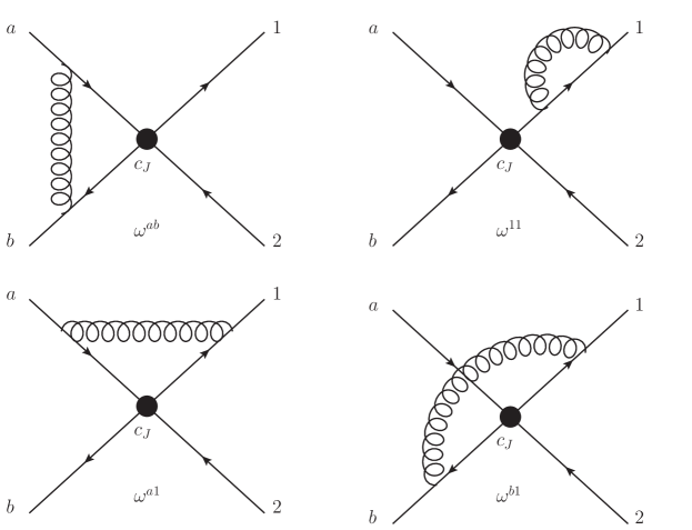
Figure 10: One-loop diagrams contributing to the soft anomalous dimension for the associated production of massive colour-octet gluinos and colour-singlet gauginos with momenta $p_{1}$ and $p_{2}$ from massless colour-triplet quarks and antiquarks with momenta $p_{a}$ and $p_{b}$. The self-energy contributions of the latter vanish.

by $k$ and $l$ the eikonal lines, between which the gluon is spanned, by $C^{kl}_{IJ}$ the colour mixing factors and by $\omega^{kl}$ the kinematic parts of the one-loop corrections, we obtain for the correction to the colour basis tensor $c_{I}$

$$\Gamma_{ab\rightarrow ij,IJ}=-\sum_{kl}C^{kl}_{IJ}{\rm Res}_{\epsilon\rightarrow 0}\omega^{kl}.$$ (41)

We compute these diagrams in an irreducible $s$-channel colour basis with tensors $c_{J}$, which one obtains in general after decomposing the reducible initial-state or final-state multi-particle product representations and which has the advantage of rendering the anomalous dimension matrices diagonal at threshold Kidonakis:1997gm ; Beenakker:2009ha . Since we have only one coloured final-state particle, the gluino with adjoint colour index $i,i^{\prime}$, there is also only one colour basis tensor $c_{J}={\rm Tr}(T^{i}T^{i^{\prime}})=T_{F}\delta_{ii^{\prime}}$ with $T_{F}=1/2$, similarly to the case of prompt photon production with an associated gluon jet Kidonakis:1999hq , and we can drop the associated indices $I,J$. At LO, it leads to the colour factor ${\rm Tr}(T^{i}T^{i})=T_{F}\delta_{ii}=C_{A}C_{F}$ computed in Sec. 2.1. At one loop and after removing the LO colour factors, we obtain for the four diagrams in Fig. 10

$$C^{ab}~{}=~{}{\operatorname{Tr}(T^{i}T^{j}T^{i}T^{j})\over\operatorname{Tr}(T^{i}T^{i})}~{}=~{}C_{F}-{C_{A}\over 2} \ ,\ C^{a1}~{}=~{}{\operatorname{Tr}(T^{i}T^{i^{\prime}}T^{j})f^{ii^{\prime}j}(-i)\over\operatorname{Tr}(T^{i}T^{i})}~{}=~{}{C_{A}\over 2},$$ (42)

$$C^{b1}~{}=~{}{\operatorname{Tr}(T^{i}T^{j}T^{i^{\prime}})f^{ii^{\prime}j}(-i)\over\operatorname{Tr}(T^{i}T^{i})}~{}=~{}-{C_{A}\over 2} \ ,\ C^{11}~{}=~{}{\operatorname{Tr}(T^{i}T^{i^{\prime}})f^{ii^{\prime\prime}j}f^{i^{\prime\prime}i^{\prime}j}(-i)^{2}\over\operatorname{Tr}(T^{i}T^{i})}~{}=~{}C_{A},\qquad~{}~{}$$

where $j$ is the colour index of the exchanged gluon.

The kinematic part of the one-loop corrections can be written in a general form as

$$\omega^{kl} = g_{s}^{2}\int\frac{\mathrm{d}^{D}q}{(2\pi)^{D}}\frac{-i}{q^{2}+i\epsilon}\biggl{[}\frac{\Delta_{k}\Delta_{l}v_{k}\cdot v_{l}}{(\delta_{k}v_{k}\cdot q+i\epsilon)(\delta_{l}v_{l}\cdot q+i\epsilon)}$$ (43)

$$- \frac{\Delta_{k}v_{k}\cdot n}{(\delta_{k}v_{k}\cdot q+i\epsilon)}\frac{P}{(n\cdot q)}-\frac{\Delta_{l}v_{l}\cdot n}{(\delta_{l}v_{l}\cdot q+i\epsilon)}\frac{P}{(n\cdot q)}+n^{2}\frac{P}{(n\cdot q)^{2}}\biggl{]}\,,$$

where $q$ is the loop momentum, $\Delta_{k,l}$ and $\delta_{k,l}$ are signs associated with the eikonal Feynman rules, and $P$ stands for the principle value Kidonakis:1997gm ; Beenakker:2009ha

$$\frac{P}{(n\cdot q)^{\beta}}=\frac{1}{2}\left(\frac{1}{(n\cdot q+i\epsilon)^{\beta}}+(-1)^{\beta}\frac{1}{(-n\cdot q+i\epsilon)^{\beta}}\right)\,.$$ (44)

The integrals can be solved Kidonakis:1997gm (also for two coloured final-state particles with unequal masses Beenakker:2009ha ) with the results Vincent

$$\omega^{ab} = S_{ab}\frac{\alpha_{s}}{\pi\epsilon}\left[-\ln{\left(\frac{v_{a}\cdot v_{b}}{2}\right)}+\frac{1}{2}\ln{\left(\frac{(v_{a}\cdot n)^{2}}{|n|^{2}}\frac{(v_{b}\cdot n)^{2}}{|n|^{2}}\right)}+i\pi-1\right],$$ (45)

$$\omega^{a1} = S_{a1}\frac{\alpha_{s}}{\pi\epsilon}\left[-\frac{1}{2}\ln{\left(\frac{(v_{a}\cdot v_{1})^{2}s}{2m_{\tilde{g}}^{2}}\right)}+L_{1}+\frac{1}{2}\ln{\left(\frac{(v_{a}\cdot n)^{2}}{|n|^{2}}\right)}-1\right],$$ (46)

$$\omega^{b1} = S_{b1}\frac{\alpha_{s}}{\pi\epsilon}\left[-\frac{1}{2}\ln{\left(\frac{(v_{b}\cdot v_{1})^{2}s}{2m_{\tilde{g}}^{2}}\right)}+L_{1}+\frac{1}{2}\ln{\left(\frac{(v_{b}\cdot n)^{2}}{|n|^{2}}\right)}-1\right],$$ (47)

$$\omega^{11} = S_{11}\frac{\alpha_{s}}{\pi\epsilon}\left[2L_{1}-2\right].$$ (48)

Here, we have combined the signs in $S_{kl}=\Delta_{k}\Delta_{l}\delta_{k}\delta_{l}$, so that $S_{ab}=1$, $S_{a1}=1$, $S_{b1}=-1$, and $S_{11}=-1$. The double poles in $\epsilon$ in the first three integrals involving at least one massless particle have canceled among themselves. As one can easily see, the scalar products are

$$v_{a}\cdot v_{b} = \frac{2p_{a}\cdot p_{b}}{s}=1\,,$$ (49)

$$v_{a}\cdot v_{1} = \frac{2p_{a}\cdot p_{1}}{s}=\frac{m_{\tilde{g}}^{2}-t}{s}\,,$$ (50)

$$v_{b}\cdot v_{1} = \frac{2p_{b}\cdot p_{1}}{s}=\frac{m_{\tilde{g}}^{2}-u}{s}\,.$$ (51)

The function $L_{k}=[L_{k}(+n)+L_{k}(-n)]/2$ depends in a rather complicated way on the gauge vector $n$ Kidonakis:1997gm ; Vincent . However, all gauge-dependent terms disappear after the inclusion of the self-energies of the two incoming Wilson lines.

Combining colour factors, signs, soft integrals and simplifying the result leads to

$${\bar{\Gamma}}_{q\bar{q}\rightarrow\tilde{g}\tilde{\chi}}=\frac{\alpha_{s}}{2\pi}C_{A}\left[\ln{2}+i\pi-1+\ln{\left(\frac{m_{\tilde{g}}^{2}-t}{\sqrt{2}m_{\tilde{g}}\sqrt{s}}\right)}+\ln{\left(\frac{m_{\tilde{g}}^{2}-u}{\sqrt{2}m_{\tilde{g}}\sqrt{s}}\right)}\right]=\frac{\alpha_{s}}{2\pi}C_{A}\left(T_{a1}+T_{b1}\right)$$ (52)

with

$$T_{a1}=\ln{\left(\frac{m_{\tilde{g}}^{2}-t}{m_{\tilde{g}}\sqrt{s}}\right)}+\frac{i\pi-1}{2} \ ,\ T_{b1}=\ln{\left(\frac{m_{\tilde{g}}^{2}-u}{m_{\tilde{g}}\sqrt{s}}\right)}+\frac{i\pi-1}{2}.$$ (53)

Due to the LSZ reduction formula, only half of the self-energy contribution $\omega^{11}$ has been taken into account. All terms proportional to $C_{F}$ have vanished, so that only terms proportional to $C_{A}$ remain. In the massless limit and before subtracting the initial-state self-energies, one recovers the well-known result for associated gluon-photon production, i.e. the $C_{A}$-term in Eq. (2.26) of Ref. Kidonakis:1999hq . Our modified soft anomalous dimension can also be compared to the one obtained for associated top-quark and $W$-boson production in Eq. (3.8) of Ref. Kidonakis:2006bu after adjustments of the colour factors. The result in Eq. (3.1) of Ref. Kidonakis:2010ux is slightly different, since Feynman gauge and not axial gauge was used there.

The final result for the soft wide-angle emission function in associated gluino-gaugino production is therefore

$$D_{q\bar{q}\rightarrow\tilde{g}\tilde{\chi}}=\operatorname{Re}\left[C_{A}\left(T_{a1}+T_{b1}\right)\right]\,.$$ (54)

At the production threshold, where the final-state particle velocities vanish and

$$\beta=\sqrt{1-\frac{(m_{\tilde{g}}+m_{\tilde{\chi}})^{2}}{s}}\rightarrow 0\,,$$ (55)

we find

$$D_{q\bar{q}\rightarrow\tilde{g}\tilde{\chi}}=-C_{A}\,,$$ (56)

in accordance with Ref. Beenakker:2009ha .

Appendix C Lists of total cross sections

In Tabs. 2 and 3 we list the total cross sections for the associated production of a second-lightest neutralino and a gluino at the LHC with a centre-of-mass energy of 13 TeV in tabular form. In Tab. 2, these cross sections are presented as a function of the gluino mass, while in Tab. 3 they are presented as a function of the wino mass parameter $M_{2}$. These tables thus correspond to Figs. 5 and 7. They also include listings of the respective scale and PDF uncertainties.

$m_{\tilde{g}}\,(\mathrm{GeV})$	$\mathrm{LO}^{+\mathrm{scale}}_{-\mathrm{scale}}\,(\mathrm{fb})$	$\mathrm{NLO}^{+\mathrm{scale}+\mathrm{PDF}}_{-\mathrm{scale}-\mathrm{PDF}}\,(\mathrm{fb})$	$\mathrm{NLL}^{+\mathrm{scale}}_{-\mathrm{scale}}\,(\mathrm{fb})$
$500$	$2.211^{+18.7\%}_{-14.8\%}$	$2.827^{+11.0\%\,+6.2\%}_{-9.5\%\,-8.1\%}$	$2.751^{+8.0\%}_{-5.8\%}$
$600$	$1.722^{+19.1\%}_{-15.1\%}$	$2.044^{+9.5\%\,+8.7\%}_{-8.7\%\,-6.8\%}$	$2.016^{+7.0\%}_{-5.2\%}$
$700$	$1.350^{+19.5\%}_{-15.3\%}$	$1.543^{+8.2\%\,+9.1\%}_{-8.4\%\,-7.3\%}$	$1.532^{+5.7\%}_{-4.8\%}$
$800$	$1.065^{+19.9\%}_{-15.5\%}$	$1.185^{+7.4\%\,+9.1\%}_{-7.9\%\,-8.8\%}$	$1.178^{+4.7\%}_{-4.2\%}$
$900$	$0.844^{+20.2\%}_{-15.8\%}$	$0.920^{+7.4\%\,+9.3\%}_{-7.8\%\,-9.4\%}$	$0.917^{+4.6\%}_{-4.0\%}$
$1000$	$0.671^{+20.5\%}_{-16.0\%}$	$0.719^{+6.7\%\,+9.6\%}_{-8.3\%\,-9.5\%}$	$0.721^{+3.8\%}_{-4.3\%}$
$1100$	$0.536^{+20.8\%}_{-16.2\%}$	$0.563^{+6.8\%\,+10.7\%}_{-7.8\%\,-9.8\%}$	$0.566^{+3.6\%}_{-3.6\%}$
$1200$	$0.429^{+21.1\%}_{-16.3\%}$	$0.444^{+6.7\%\,+10.1\%}_{-7.6\%\,-11.3\%}$	$0.447^{+3.2\%}_{-3.4\%}$
$1300$	$0.344^{+21.4\%}_{-16.5\%}$	$0.350^{+6.6\%\,+11.4\%}_{-7.3\%\,-11.1\%}$	$0.353^{+3.0\%}_{-2.9\%}$
$1400$	$0.277^{+21.6\%}_{-16.7\%}$	$0.277^{+6.2\%\,+11.6\%}_{-7.6\%\,-12.2\%}$	$0.280^{+2.5\%}_{-3.1\%}$
$1500$	$0.224^{+21.9\%}_{-16.9\%}$	$0.220^{+6.7\%\,+11.7\%}_{-7.3\%\,-13.3\%}$	$0.223^{+2.9\%}_{-2.7\%}$
$1600$	$0.180^{+22.2\%}_{-17.0\%}$	$0.174^{+6.4\%\,+13.4\%}_{-6.8\%\,-12.9\%}$	$0.177^{+2.3\%}_{-2.1\%}$
$1700$	$0.146^{+22.4\%}_{-17.2\%}$	$0.139^{+5.6\%\,+14.2\%}_{-7.1\%\,-13.6\%}$	$0.141^{+1.5\%}_{-2.2\%}$
$1800$	$0.118^{+22.7\%}_{-17.4\%}$	$0.110^{+5.4\%\,+15.0\%}_{-7.1\%\,-14.3\%}$	$0.113^{+1.3\%}_{-2.1\%}$
$1900$	$0.096^{+22.9\%}_{-17.5\%}$	$0.088^{+5.7\%\,+15.6\%}_{-7.1\%\,-15.1\%}$	$0.090^{+1.3\%}_{-2.0\%}$
$2000$	$0.078^{+23.2\%}_{-17.7\%}$	$0.071^{+5.4\%\,+16.4\%}_{-6.9\%\,-16.1\%}$	$0.073^{+1.0\%}_{-1.7\%}$
$2100$	$0.063^{+23.4\%}_{-17.8\%}$	$0.057^{+5.4\%\,+17.9\%}_{-7.3\%\,-16.2\%}$	$0.059^{+0.9\%}_{-1.9\%}$
$2200$	$0.051^{+23.7\%}_{-18.0\%}$	$0.046^{+5.4\%\,+18.2\%}_{-7.3\%\,-17.3\%}$	$0.048^{+0.7\%}_{-1.8\%}$
$2300$	$0.042^{+23.9\%}_{-18.1\%}$	$0.037^{+5.6\%\,+19.3\%}_{-7.2\%\,-18.0\%}$	$0.038^{+1.0\%}_{-1.6\%}$
$2400$	$0.034^{+24.1\%}_{-18.3\%}$	$0.030^{+5.6\%\,+20.3\%}_{-7.3\%\,-18.8\%}$	$0.031^{+1.0\%}_{-1.7\%}$
$2500$	$0.028^{+24.4\%}_{-18.4\%}$	$0.024^{+5.7\%\,+21.3\%}_{-7.6\%\,-19.7\%}$	$0.025^{+0.8\%}_{-1.8\%}$
$2600$	$0.022^{+24.6\%}_{-18.5\%}$	$0.019^{+5.9\%\,+22.8\%}_{-7.6\%\,-20.4\%}$	$0.020^{+0.9\%}_{-1.7\%}$
$2700$	$0.018^{+24.8\%}_{-18.7\%}$	$0.016^{+6.1\%\,+23.4\%}_{-7.8\%\,-21.7\%}$	$0.017^{+0.8\%}_{-1.8\%}$
$2800$	$0.015^{+25.1\%}_{-18.9\%}$	$0.013^{+6.3\%\,+24.9\%}_{-8.1\%\,-22.4\%}$	$0.013^{+0.7\%}_{-1.8\%}$
$2900$	$0.012^{+25.3\%}_{-19.0\%}$	$0.010^{+6.4\%\,+26.3\%}_{-8.2\%\,-23.3\%}$	$0.011^{+0.7\%}_{-1.8\%}$
$3000$	$0.010^{+25.5\%}_{-19.2\%}$	$0.008^{+6.6\%\,+27.7\%}_{-8.3\%\,-24.3\%}$	$0.009^{+0.6\%}_{-1.8\%}$

Table 2: Total cross sections for $p\,p\rightarrow\tilde{\chi}_{2}^{0}\,\tilde{g}$ at $\sqrt{S}=13\,\mathrm{TeV}$ as a function of the gluino mass $m_{\tilde{g}}$ using CT14NLO PDFs.

$M_{2}=2\,M_{1}\,(\mathrm{GeV})$	$\mathrm{LO}^{+\mathrm{scale}}_{-\mathrm{scale}}\,(\mathrm{fb})$	$\mathrm{NLO}^{+\mathrm{scale}+\mathrm{PDF}}_{-\mathrm{scale}-\mathrm{PDF}}\,(\mathrm{fb})$	$\mathrm{NLL}^{+\mathrm{scale}}_{-\mathrm{scale}}\,(\mathrm{fb})$
$100$	$0.309^{+21.9\%}_{-16.9\%}$	$0.272^{+2.7\%\,+13.0\%}_{-5.4\%\,-13.2\%}$	$0.277^{+0.6\%}_{-0.9\%}$
$150$	$0.271^{+22.0\%}_{-17.0\%}$	$0.239^{+3.0\%\,+13.9\%}_{-5.6\%\,-13.3\%}$	$0.245^{+0.6\%}_{-1.1\%}$
$200$	$0.238^{+22.2\%}_{-17.0\%}$	$0.211^{+3.4\%\,+13.7\%}_{-5.6\%\,-14.0\%}$	$0.215^{+0.7\%}_{-1.0\%}$
$250$	$0.208^{+22.3\%}_{-17.1\%}$	$0.185^{+3.5\%\,+14.4\%}_{-5.9\%\,-13.9\%}$	$0.189^{+0.6\%}_{-1.1\%}$
$300$	$0.182^{+22.4\%}_{-17.2\%}$	$0.162^{+3.8\%\,+14.9\%}_{-6.2\%\,-13.9\%}$	$0.166^{+0.7\%}_{-1.4\%}$
$350$	$0.159^{+22.6\%}_{-17.3\%}$	$0.142^{+4.3\%\,+14.6\%}_{-6.1\%\,-14.8\%}$	$0.145^{+0.8\%}_{-1.2\%}$
$400$	$0.139^{+22.7\%}_{-17.4\%}$	$0.124^{+4.3\%\,+15.2\%}_{-6.3\%\,-14.9\%}$	$0.128^{+0.8\%}_{-1.3\%}$
$450$	$0.121^{+22.8\%}_{-17.5\%}$	$0.109^{+4.6\%\,+15.7\%}_{-6.6\%\,-15.3\%}$	$0.112^{+0.8\%}_{-1.6\%}$
$500$	$0.105^{+23.0\%}_{-17.5\%}$	$0.095^{+4.7\%\,+16.2\%}_{-6.8\%\,-15.2\%}$	$0.098^{+0.7\%}_{-1.7\%}$
$550$	$0.092^{+23.1\%}_{-17.6\%}$	$0.083^{+4.9\%\,+16.5\%}_{-6.8\%\,-15.4\%}$	$0.085^{+0.8\%}_{-1.7\%}$
$600$	$0.078^{+23.2\%}_{-17.7\%}$	$0.071^{+5.1\%\,+16.9\%}_{-7.0\%\,-15.7\%}$	$0.073^{+0.9\%}_{-1.8\%}$
$650$	$0.065^{+23.3\%}_{-17.8\%}$	$0.059^{+5.5\%\,+17.0\%}_{-7.2\%\,-16.4\%}$	$0.061^{+0.9\%}_{-1.9\%}$
$700$	$0.051^{+23.4\%}_{-17.8\%}$	$0.046^{+6.0\%\,+18.4\%}_{-7.1\%\,-15.7\%}$	$0.048^{+1.4\%}_{-1.8\%}$
$750$	$0.036^{+23.4\%}_{-17.8\%}$	$0.032^{+5.8\%\,+18.3\%}_{-7.4\%\,-16.1\%}$	$0.033^{+1.0\%}_{-1.9\%}$
$800$	$0.022^{+23.4\%}_{-17.8\%}$	$0.020^{+5.8\%\,+17.9\%}_{-7.4\%\,-16.7\%}$	$0.020^{+1.0\%}_{-1.9\%}$
$850$	$0.013^{+23.3\%}_{-17.8\%}$	$0.012^{+6.0\%\,+18.8\%}_{-7.5\%\,-16.1\%}$	$0.012^{+1.1\%}_{-1.9\%}$
$900$	$0.008^{+23.1\%}_{-17.7\%}$	$0.007^{+5.8\%\,+18.2\%}_{-7.4\%\,-16.8\%}$	$0.008^{+0.8\%}_{-1.8\%}$
$950$	$0.005^{+22.9\%}_{-17.5\%}$	$0.005^{+5.9\%\,+17.9\%}_{-7.2\%\,-17.1\%}$	$0.005^{+0.8\%}_{-1.5\%}$
$1000$	$0.004^{+22.7\%}_{-17.4\%}$	$0.004^{+5.9\%\,+18.8\%}_{-7.3\%\,-16.5\%}$	$0.004^{+0.7\%}_{-1.5\%}$
$1050$	$0.004^{+22.5\%}_{-17.3\%}$	$0.003^{+5.8\%\,+18.8\%}_{-7.1\%\,-16.5\%}$	$0.003^{+0.5\%}_{-1.4\%}$
$1100$	$0.003^{+22.3\%}_{-17.2\%}$	$0.003^{+6.0\%\,+18.9\%}_{-7.2\%\,-16.5\%}$	$0.003^{+0.7\%}_{-1.4\%}$
$1150$	$0.003^{+22.3\%}_{-17.2\%}$	$0.003^{+6.0\%\,+18.9\%}_{-7.2\%\,-16.6\%}$	$0.003^{+0.7\%}_{-1.5\%}$
$1200$	$0.003^{+22.3\%}_{-17.2\%}$	$0.003^{+6.1\%\,+18.9\%}_{-7.2\%\,-16.2\%}$	$0.003^{+0.8\%}_{-1.4\%}$
$1250$	$0.003^{+22.4\%}_{-17.2\%}$	$0.003^{+6.2\%\,+18.9\%}_{-7.4\%\,-16.1\%}$	$0.003^{+0.8\%}_{-1.6\%}$
$1300$	$0.004^{+22.6\%}_{-17.3\%}$	$0.004^{+6.3\%\,+18.7\%}_{-7.6\%\,-16.0\%}$	$0.004^{+0.7\%}_{-1.8\%}$

Table 3: Total cross sections for $p\,p\rightarrow\tilde{\chi}_{2}^{0}\,\tilde{g}$ at $\sqrt{S}=13\,\mathrm{TeV}$ as a function of the wino mass parameter $M_{2}$ using CT14NLO PDFs.

References

- (1) ATLAS Collaboration, G. Aad et. al., Search for new phenomena in final states with large jet multiplicities and missing transverse momentum with ATLAS using TeV proton–proton collisions, 1602.06194.
- (2) CMS Collaboration, C. Collaboration, Search for SUSY in same-sign dilepton events at TeV, CMS-PAS-SUS-15-008.
- (3) ATLAS Collaboration, G. Aad et. al., Search for direct production of charginos, neutralinos and sleptons in final states with two leptons and missing transverse momentum in collisions at 8 TeV with the ATLAS detector, JHEP 05 (2014) 071, [1403.5294].
- (4) CMS Collaboration, V. Khachatryan et. al., Searches for electroweak production of charginos, neutralinos, and sleptons decaying to leptons and W, Z, and Higgs bosons in pp collisions at 8 TeV, Eur. Phys. J. C74 (2014), no. 9 3036, [1405.7570].
- (5) S. Dawson, E. Eichten, and C. Quigg, Search for Supersymmetric Particles in Hadron - Hadron Collisions, Phys. Rev. D31 (1985) 1581.
- (6) H. Baer, D. D. Karatas, and X. Tata, Gluino and Squark Production in Association With Gauginos at Hadron Supercolliders, Phys. Rev. D42 (1990) 2259–2264.
- (7) M. Klasen and G. Pignol, New Results for Light Gravitinos at Hadron Colliders: Tevatron Limits and LHC Perspectives, Phys. Rev. D75 (2007) 115003, [hep-ph/0610160].
- (8) W. Beenakker, R. Höpker, and M. Spira, PROSPINO: A Program for the production of supersymmetric particles in next-to-leading order QCD, hep-ph/9611232.
- (9) E. L. Berger, M. Klasen, and T. M. P. Tait, Scale dependence of squark and gluino production cross-sections, Phys. Rev. D59 (1999) 074024, [hep-ph/9807230].
- (10) W. Beenakker, M. Klasen, M. Krämer, T. Plehn, M. Spira, and P. M. Zerwas, The Production of charginos / neutralinos and sleptons at hadron colliders, Phys. Rev. Lett. 83 (1999) 3780–3783, [hep-ph/9906298]. [Erratum: Phys. Rev. Lett.100,029901(2008)].
- (11) M. Spira, Higgs and SUSY particle production at hadron colliders, in Supersymmetry and unification of fundamental interactions. Proceedings, 10th International Conference, SUSY’02, Hamburg, Germany, June 17-23, 2002, pp. 217–226, 2002. hep-ph/0211145.
- (12) E. L. Berger, M. Klasen, and T. M. P. Tait, Associated production of gauginos and gluinos at hadron colliders in next-to-leading order SUSY QCD, Phys. Lett. B459 (1999) 165–170, [hep-ph/9902350].
- (13) E. L. Berger, M. Klasen, and T. M. P. Tait, Next-to-leading order SUSY QCD predictions for associated production of gauginos and gluinos, Phys. Rev. D62 (2000) 095014, [hep-ph/0005196].
- (14) E. L. Berger, M. Klasen, and T. M. P. Tait, Erratum: Next-to-leading order supersymmetric QCD predictions for associated production of gauginos and gluinos (Phys.Rev.D62:095014,2000), Phys. Rev. D67 (2003) 099901, [hep-ph/0212306].
- (15) D. Goncalves-Netto, D. Lopez-Val, K. Mawatari, T. Plehn, and I. Wigmore, Automated Squark and Gluino Production to Next-to-Leading Order, Phys. Rev. D87 (2013), no. 1 014002, [1211.0286].
- (16) T. Binoth, D. Goncalves Netto, D. Lopez-Val, K. Mawatari, T. Plehn, and I. Wigmore, Automized Squark-Neutralino Production to Next-to-Leading Order, Phys. Rev. D84 (2011) 075005, [1108.1250].
- (17) D. Goncalves, D. Lopez-Val, K. Mawatari, and T. Plehn, Automated third generation squark production to next-to-leading order, Phys. Rev. D90 (2014), no. 7 075007, [1407.4302].
- (18) C. Degrande, B. Fuks, V. Hirschi, J. Proudom, and H.-S. Shao, Automated next-to-leading order predictions for new physics at the LHC: the case of colored scalar pair production, Phys. Rev. D91 (2015), no. 9 094005, [1412.5589].
- (19) C. Degrande, B. Fuks, V. Hirschi, J. Proudom, and H.-S. Shao, Matching next-to-leading order predictions to parton showers in supersymmetric QCD, Phys. Lett. B755 (2016) 82–87, [1510.00391].
- (20) G. F. Sterman, Summation of Large Corrections to Short Distance Hadronic Cross-Sections, Nucl. Phys. B281 (1987) 310.
- (21) N. Kidonakis and G. F. Sterman, Resummation for QCD hard scattering, Nucl. Phys. B505 (1997) 321–348, [hep-ph/9705234].
- (22) N. Kidonakis, G. Oderda, and G. F. Sterman, Threshold resummation for dijet cross-sections, Nucl. Phys. B525 (1998) 299–332, [hep-ph/9801268].
- (23) S. Catani and L. Trentadue, Resummation of the QCD Perturbative Series for Hard Processes, Nucl. Phys. B327 (1989) 323.
- (24) S. Catani and L. Trentadue, Comment on QCD exponentiation at large x, Nucl. Phys. B353 (1991) 183–186.
- (25) G. Bozzi, B. Fuks, and M. Klasen, Slepton production in polarized hadron collisions, Phys. Lett. B609 (2005) 339–350, [hep-ph/0411318].
- (26) G. Bozzi, B. Fuks, and M. Klasen, Transverse-momentum resummation for slepton-pair production at the CERN LHC, Phys. Rev. D74 (2006) 015001, [hep-ph/0603074].
- (27) G. Bozzi, B. Fuks, and M. Klasen, Threshold Resummation for Slepton-Pair Production at Hadron Colliders, Nucl. Phys. B777 (2007) 157–181, [hep-ph/0701202].
- (28) G. Bozzi, B. Fuks, and M. Klasen, Joint resummation for slepton pair production at hadron colliders, Nucl. Phys. B794 (2008) 46–60, [0709.3057].
- (29) B. Fuks, M. Klasen, D. R. Lamprea, and M. Rothering, Revisiting slepton pair production at the Large Hadron Collider, JHEP 01 (2014) 168, [1310.2621].
- (30) J. Debove, B. Fuks, and M. Klasen, Model-independent analysis of gaugino-pair production in polarized and unpolarized hadron collisions, Phys. Rev. D78 (2008) 074020, [0804.0423].
- (31) J. Debove, B. Fuks, and M. Klasen, Transverse-momentum resummation for gaugino-pair production at hadron colliders, Phys. Lett. B688 (2010) 208–211, [0907.1105].
- (32) J. Debove, B. Fuks, and M. Klasen, Threshold resummation for gaugino pair production at hadron colliders, Nucl. Phys. B842 (2011) 51–85, [1005.2909].
- (33) J. Debove, B. Fuks, and M. Klasen, Joint Resummation for Gaugino Pair Production at Hadron Colliders, Nucl. Phys. B849 (2011) 64–79, [1102.4422].
- (34) B. Fuks, M. Klasen, D. R. Lamprea, and M. Rothering, Gaugino production in proton-proton collisions at a center-of-mass energy of 8 TeV, JHEP 10 (2012) 081, [1207.2159].
- (35) B. Fuks, M. Klasen, D. R. Lamprea, and M. Rothering, Precision predictions for electroweak superpartner production at hadron colliders with Resummino, Eur. Phys. J. C73 (2013) 2480, [1304.0790].
- (36) A. Kulesza and L. Motyka, Threshold resummation for squark-antisquark and gluino-pair production at the LHC, Phys. Rev. Lett. 102 (2009) 111802, [0807.2405].
- (37) U. Langenfeld and S.-O. Moch, Higher-order soft corrections to squark hadro-production, Phys. Lett. B675 (2009) 210–221, [0901.0802].
- (38) P. Falgari, C. Schwinn, and C. Wever, NLL soft and Coulomb resummation for squark and gluino production at the LHC, JHEP 06 (2012) 052, [1202.2260].
- (39) U. Langenfeld, S.-O. Moch, and T. Pfoh, QCD threshold corrections for gluino pair production at hadron colliders, JHEP 11 (2012) 070, [1208.4281].
- (40) W. Beenakker, S. Brensing, M. Krämer, A. Kulesza, E. Laenen, and I. Niessen, Soft-gluon resummation for squark and gluino hadroproduction, JHEP 12 (2009) 041, [0909.4418].
- (41) W. Beenakker, S. Brensing, M. Krämer, A. Kulesza, E. Laenen, and I. Niessen, NNLL resummation for squark-antisquark pair production at the LHC, JHEP 01 (2012) 076, [1110.2446].
- (42) W. Beenakker, T. Janssen, S. Lepoeter, M. Krämer, A. Kulesza, E. Laenen, I. Niessen, S. Thewes, and T. Van Daal, Towards NNLL resummation: hard matching coefficients for squark and gluino hadroproduction, JHEP 10 (2013) 120, [1304.6354].
- (43) M. Beneke, P. Falgari, and C. Schwinn, Threshold resummation for pair production of coloured heavy (s)particles at hadron colliders, Nucl. Phys. B842 (2011) 414–474, [1007.5414].
- (44) A. Broggio, M. Neubert, and L. Vernazza, Soft-gluon resummation for slepton-pair production at hadron colliders, JHEP 05 (2012) 151, [1111.6624].
- (45) A. Broggio, A. Ferroglia, M. Neubert, L. Vernazza, and L. L. Yang, NNLL Momentum-Space Resummation for Stop-Pair Production at the LHC, JHEP 03 (2014) 066, [1312.4540].
- (46) A. Broggio, A. Ferroglia, M. Neubert, L. Vernazza, and L. L. Yang, Approximate NNLO Predictions for the Stop-Pair Production Cross Section at the LHC, JHEP 07 (2013) 042, [1304.2411].
- (47) T. Pfoh, Phenomenology of QCD threshold resummation for gluino pair production at NNLL, JHEP 05 (2013) 044, [1302.7202]. [Erratum: JHEP10,090(2013)].
- (48) W. Beenakker, C. Borschensky, M. Krämer, A. Kulesza, E. Laenen, V. Theeuwes, and S. Thewes, NNLL resummation for squark and gluino production at the LHC, JHEP 12 (2014) 023, [1404.3134].
- (49) W. Beenakker, C. Borschensky, R. Heger, M. Krämer, A. Kulesza, and E. Laenen, NNLL resummation for stop pair-production at the LHC, JHEP 05 (2016) 153, [1601.02954].
- (50) M. Bonvini, S. Forte, M. Ghezzi, and G. Ridolfi, Threshold Resummation in SCET vs. Perturbative QCD: An Analytic Comparison, Nucl. Phys. B861 (2012) 337–360, [1201.6364].
- (51) M. Bonvini, S. Forte, G. Ridolfi, and L. Rottoli, Resummation prescriptions and ambiguities in SCET vs. direct QCD: Higgs production as a case study, JHEP 01 (2015) 046, [1409.0864].
- (52) B. Jäger, A. von Manteuffel, and S. Thier, Slepton pair production in the POWHEG BOX, JHEP 10 (2012) 130, [1208.2953].
- (53) B. Jäger, A. von Manteuffel, and S. Thier, Slepton pair production in association with a jet: NLO-QCD corrections and parton-shower effects, JHEP 02 (2015) 041, [1410.3802].
- (54) R. Gavin, C. Hangst, M. Krämer, M. Mühlleitner, M. Pellen, E. Popenda, and M. Spira, Matching Squark Pair Production at NLO with Parton Showers, JHEP 10 (2013) 187, [1305.4061].
- (55) R. Gavin, C. Hangst, M. Krämer, M. Mühlleitner, M. Pellen, E. Popenda, and M. Spira, Squark Production and Decay matched with Parton Showers at NLO, Eur. Phys. J. C75 (2015), no. 1 29, [1407.7971].
- (56) J. Baglio, B. Jäger, and M. Kesenheimer, Electroweakino pair production at the LHC: NLO SUSY-QCD corrections and parton-shower effects, 1605.06509.
- (57) B. Fuks, M. Klasen, F. Ledroit, Q. Li, and J. Morel, Precision predictions for - production at the CERN LHC: QCD matrix elements, parton showers, and joint resummation, Nucl. Phys. B797 (2008) 322–339, [0711.0749].
- (58) C. Weydert, S. Frixione, M. Herquet, M. Klasen, E. Laenen, T. Plehn, G. Stavenga, and C. D. White, Charged Higgs boson production in association with a top quark in MC@NLO, Eur. Phys. J. C67 (2010) 617–636, [0912.3430].
- (59) M. Klasen, K. Kovarik, P. Nason, and C. Weydert, Associated production of charged Higgs bosons and top quarks with POWHEG, Eur. Phys. J. C72 (2012) 2088, [1203.1341].
- (60) R. Bonciani, T. Jezo, M. Klasen, F. Lyonnet, and I. Schienbein, Electroweak top-quark pair production at the LHC with bosons to NLO QCD in POWHEG, JHEP 02 (2016) 141, [1511.08185].
- (61) G. Bozzi, B. Fuks, and M. Klasen, Non-diagonal and mixed squark production at hadron colliders, Phys. Rev. D72 (2005) 035016, [hep-ph/0507073].
- (62) G. Bozzi, B. Fuks, B. Herrmann, and M. Klasen, Squark and gaugino hadroproduction and decays in non-minimal flavour violating supersymmetry, Nucl. Phys. B787 (2007) 1–54, [0704.1826].
- (63) F. del Aguila et. al., Collider aspects of flavour physics at high , Eur. Phys. J. C57 (2008) 183–308, [0801.1800].
- (64) B. Fuks, B. Herrmann, and M. Klasen, Flavour Violation in Gauge-Mediated Supersymmetry Breaking Models: Experimental Constraints and Phenomenology at the LHC, Nucl. Phys. B810 (2009) 266–299, [0808.1104].
- (65) B. Fuks, B. Herrmann, and M. Klasen, Phenomenology of anomaly-mediated supersymmetry breaking scenarios with non-minimal flavour violation, Phys. Rev. D86 (2012) 015002, [1112.4838].
- (66) K. De Causmaecker, B. Fuks, B. Herrmann, F. Mahmoudi, B. O’Leary, W. Porod, S. Sekmen, and N. Strobbe, General squark flavour mixing: constraints, phenomenology and benchmarks, JHEP 11 (2015) 125, [1509.05414].
- (67) J. C. Collins, D. E. Soper, and G. F. Sterman, Factorization of Hard Processes in QCD, Adv. Ser. Direct. High Energy Phys. 5 (1989) 1–91, [hep-ph/0409313].
- (68) S. P. Martin and M. T. Vaughn, Regularization dependence of running couplings in softly broken supersymmetry, Phys. Lett. B318 (1993) 331–337, [hep-ph/9308222].
- (69) S. Catani and M. Seymour, The Dipole formalism for the calculation of QCD jet cross-sections at next-to-leading order, Phys.Lett. B378 (1996) 287–301, [hep-ph/9602277].
- (70) S. Catani, S. Dittmaier, M. H. Seymour, and Z. Trocsanyi, The Dipole formalism for next-to-leading order QCD calculations with massive partons, Nucl.Phys. B627 (2002) 189–265, [hep-ph/0201036].
- (71) T. Kinoshita, Mass singularities of Feynman amplitudes, J. Math. Phys. 3 (1962) 650–677.
- (72) T. D. Lee and M. Nauenberg, Degenerate Systems and Mass Singularities, Phys. Rev. 133 (1964) B1549–B1562.
- (73) A. Vogt, Next-to-next-to-leading logarithmic threshold resummation for deep inelastic scattering and the Drell-Yan process, Phys. Lett. B497 (2001) 228–234, [hep-ph/0010146].
- (74) M. Krämer, E. Laenen, and M. Spira, Soft gluon radiation in Higgs boson production at the LHC, Nucl. Phys. B511 (1998) 523–549, [hep-ph/9611272].
- (75) S. Catani, D. de Florian, and M. Grazzini, Higgs production in hadron collisions: Soft and virtual QCD corrections at NNLO, JHEP 05 (2001) 025, [hep-ph/0102227].
- (76) T. O. Eynck, E. Laenen, and L. Magnea, Exponentiation of the Drell-Yan cross-section near partonic threshold in the DIS and MS-bar schemes, JHEP 06 (2003) 057, [hep-ph/0305179].
- (77) H. Contopanagos and G. F. Sterman, Principal value resummation, Nucl. Phys. B419 (1994) 77–104, [hep-ph/9310313].
- (78) S. Catani, M. L. Mangano, P. Nason, and L. Trentadue, The Resummation of soft gluons in hadronic collisions, Nucl. Phys. B478 (1996) 273–310, [hep-ph/9604351].
- (79) A. D. Martin, W. J. Stirling, R. S. Thorne, and G. Watt, Parton distributions for the LHC, Eur. Phys. J. C63 (2009) 189–285, [0901.0002].
- (80) S. Dulat, T.-J. Hou, J. Gao, M. Guzzi, J. Huston, P. Nadolsky, J. Pumplin, C. Schmidt, D. Stump, and C. P. Yuan, New parton distribution functions from a global analysis of quantum chromodynamics, Phys. Rev. D93 (2016), no. 3 033006, [1506.07443].
- (81) NNPDF Collaboration, R. D. Ball et. al., Parton distributions for the LHC Run II, JHEP 04 (2015) 040, [1410.8849].
- (82) Particle Data Group Collaboration, K. A. Olive et. al., Review of Particle Physics, Chin. Phys. C38 (2014) 090001.
- (83) M. Klasen, M. Pohl, and G. Sigl, Indirect and direct search for dark matter, Prog. Part. Nucl. Phys. 85 (2015) 1–32, [1507.03800].
- (84) J. Harz, B. Herrmann, M. Klasen, K. Kovarik, and Q. L. Boulc’h, Neutralino-stop coannihilation into electroweak gauge and Higgs bosons at one loop, Phys. Rev. D87 (2013), no. 5 054031, [1212.5241].
- (85) J. Harz, B. Herrmann, M. Klasen, and K. Kovarik, One-loop corrections to neutralino-stop coannihilation revisited, Phys. Rev. D91 (2015), no. 3 034028, [1409.2898].
- (86) J. Harz, B. Herrmann, M. Klasen, K. Kovarik, and M. Meinecke, SUSY-QCD corrections to stop annihilation into electroweak final states including Coulomb enhancement effects, Phys. Rev. D91 (2015), no. 3 034012, [1410.8063].
- (87) J. Harz, B. Herrmann, M. Klasen, K. Kovarik, and P. Steppeler, Theoretical uncertainty of the supersymmetric dark matter relic density from scheme and scale variations, 1602.08103.
- (88) W. Porod and F. Staub, SPheno 3.1: Extensions including flavour, CP-phases and models beyond the MSSM, Comput. Phys. Commun. 183 (2012) 2458–2469, [1104.1573].
- (89) M. Bonvini, S. Marzani, J. Rojo, L. Rottoli, M. Ubiali, R. D. Ball, V. Bertone, S. Carrazza, and N. P. Hartland, Parton distributions with threshold resummation, JHEP 09 (2015) 191, [1507.01006].
- (90) W. Beenakker, C. Borschensky, M. Krämer, A. Kulesza, E. Laenen, S. Marzani, and J. Rojo, NLO+NLL squark and gluino production cross-sections with threshold-improved parton distributions, Eur. Phys. J. C76 (2016), no. 2 53, [1510.00375].
- (91) S. Profumo and C. E. Yaguna, Gluino coannihilations and heavy bino dark matter, Phys. Rev. D69 (2004) 115009, [hep-ph/0402208].
- (92) N. Nagata, H. Otono, and S. Shirai, Probing bino–gluino coannihilation at the LHC, Phys. Lett. B748 (2015) 24–29, [1504.00504].
- (93) J. Ellis, J. L. Evans, F. Luo, and K. A. Olive, Scenarios for Gluino Coannihilation, JHEP 02 (2016) 071, [1510.03498].
- (94) P. Nath and A. B. Spisak, Gluino Coannihilation and Observability of Gluinos at LHC RUN II, 1603.04854.
- (95) H. E. Haber and G. L. Kane, The Search for Supersymmetry: Probing Physics Beyond the Standard Model, Phys. Rept. 117 (1985) 75–263.
- (96) J. F. Gunion and H. E. Haber, Higgs Bosons in Supersymmetric Models. 1., Nucl. Phys. B272 (1986) 1. [Erratum: Nucl. Phys.B402,567(1993)].
- (97) N. Kidonakis and J. F. Owens, Soft gluon resummation and NNLO corrections for direct photon production, Phys. Rev. D61 (2000) 094004, [hep-ph/9912388].
- (98) V. M. Theeuwes, Soft Gluon Resummation for Heavy Particle Production at the Large Hadron Collider. PhD thesis, Westfälische Wilhelms-Universität, Münster, 2015.
- (99) N. Kidonakis, Single top production at the Tevatron: Threshold resummation and finite-order soft gluon corrections, Phys. Rev. D74 (2006) 114012, [hep-ph/0609287].
- (100) N. Kidonakis, Two-loop soft anomalous dimensions for single top quark associated production with a W- or H-, Phys. Rev. D82 (2010) 054018, [1005.4451].