A general multiple-relaxation-time lattice Boltzmann model for nonlinear anisotropic convection-diffusion equations

Abstract

In this paper, based on the previous work [B. Shi, Z. Guo, Lattice Boltzmann model for nonlinear convection-diffusion equations, Phys. Rev. E 79 (2009) 016701], we develop a general multiple-relaxation-time (MRT) lattice Boltzmann model for nonlinear anisotropic convection-diffusion equation (NACDE), and show that the NACDE can be recovered correctly from the present model through the Chapman-Enskog analysis. We then test the MRT model through some classic CDEs, and find that the numerical results are in good agreement with analytical solutions or some available results. Besides, the numerical results also show that similar to the single-relaxation-time (SRT) lattice Boltzmann model or so-called BGK model, the present MRT model also has a second-order convergence rate in space. Finally, we also perform a comparative study on the accuracy and stability of the MRT model and BGK model by using two examples. In terms of the accuracy, both the theoretical analysis and numerical results show that a numerical slip on the boundary would be caused in the BGK model, and cannot be eliminated unless the relaxation parameter is fixed to be a special value, while the numerical slip in the MRT model can be overcome once the relaxation parameters satisfy some constrains. The results in terms of stability also demonstrate that the MRT model could be more stable than the BGK model through tuning the free relaxation parameters.

1 Introduction

In the past decades, the lattice Boltzmann (LB) method, as a numerical approach originated from the lattice gas automata or developed from the simplified kinetic models, has gained great success in the simulation of the complex flows [1, 2, 3, 4], and has also been extended to solve some partial differential equations, including the diffusion equation [5, 6], wave equation [7], Burgers equation [8], Poisson equation [9], isotropic and anisotropic convection-diffusion equations (CDEs) [10, 11, 12, 13, 25, 14, 26, 15, 16, 17, 18, 19, 20, 27, 28, 29, 30, 31, 32, 21, 33, 34, 22, 23, 24, 35, 36]. However, most of these available works related to CDEs mainly focused on the linear CDE for its important role in the study of the heat and mass transfer [10, 11, 12, 13, 25, 14, 26, 15, 16, 17, 18, 19, 20, 27, 28, 29, 30, 31, 32, 21, 33, 34, 22, 23, 24]. Recently, through constructing a proper equilibrium distribution function, Shi and Guo [35] proposed a single-relaxation-time (SRT) LB model or the Bhatnagar-Gross-Krook (BGK) model for nonlinear convection-diffusion equations (NCDEs) where a nonlinear convection and/or diffusion term is included. Although the model has a second-order convergence rate in space [35, 36], and can also be considered as an extension to some available works, it still has some limitations. The first is that when the BGK model is used to solve the NCDEs where the diffusion coefficient is very small, the relaxation parameter would be close to its limit value, thus the model may suffer from the stability or accuracy problem [32, 22]. Secondly, the BGK model is usually limited to solve the nonlinear isotropic CDEs since it does not have sufficient relaxation parameters to describe the anisotropic diffusion process, while the multiple-relaxation-time (MRT) LB model with more relaxation parameters seems more suitable and more reasonable in solving NCDE with anisotropic diffusion process. And finally, it is also well known that in the BGK model, only a single relaxation process is used to characterize the collision effects, which means all modes relax to their equilibria with the same rate, while from a physical point of view, these rates corresponding to different modes should be different from each other during the collision process [4, 37]. To overcome these deficiencies inherent in the BGK model, in this work we will present a general MRT LB model for the nonlinear anisotropic CDE (NACDE), and show that, through the Chapman-Enskog analysis, the NACDE with a source term can be recovered correctly from the proposed model. Besides, it is also found that, similar to our previous BGK model [35, 36], the present MRT model also has a second-order convergence rate in space, while it could be more stable and more accurate than the BGK model through tuning the relaxation parameters properly.

The rest of the paper is organized as follows. In section 2, a general MRT model for NACDE with a source term is first presented, and then some special cases and distinct characteristics of the present model are also discussed. In section 3, the accuracy and convergence rate of the MRT model are tested through some classic CDEs, followed by a comparison between the present MRT model and the BGK model, and finally, some conclusions are given in section 4.

2 Multiple-relaxation-time lattice Boltzmann model for nonlinear anisotropic convection-diffusion equations

2.1 Nonlinear anisotropic convection-diffusion equation

The $n$-dimensional ($n$-D) nonlinear anisotropic convection-diffusion equation with a source term can be written as

$$\partial_{t}\phi+\nabla\cdot\mathbf{B}(\phi)=\nabla\cdot[\mathbf{K}\cdot(\nabla\cdot\mathbf{D}(\phi))]+R(\mathbf{x},t),$$ (1)

where $\phi$ is a scalar variable and is a function of time and space, $\nabla$ is the gradient operator, $\mathbf{K}=\mathbf{K}(\phi,\mathbf{x},t)$ is the diffusion tensor. $\mathbf{B}(\phi)$ and $\mathbf{D}(\phi)$ are two differential tensor functions with respect to $\phi$, $R(\mathbf{x},t)$ is the source term. It should be noted that Eq. (1) can be viewed as a general form of some important partial differential equations [32, 35, 36], such as the (anisotropic) diffusion equation, Burgers equation, Burgers-Fisher equation, Buckley-Leverett equation, nonlinear heat conduction equation, (anisotropic) convection-diffusion equation, and so on.

2.2 Multiple-relaxation-time lattice Boltzmann model

Generally, the models in the LB method can be classified into three kinds based on collision operator, i.e., the lattice BGK model [38, 39], the two relaxation-time model [29, 40], and the MRT model [37, 41]. In this work, we will focus on the MRT model for its superiority on the stability and accuracy both in the study of fluid flows [37, 42] and solving CDEs [32, 22].

The MRT model with D$n$Q$q$ lattice ($q$ is the number of discrete directions) [38] for the NACDE [Eq. (1)] is considered here, and the evolution equation of the model can be written as

$$\phi_{k}(\mathbf{x}+\mathbf{c}_{k}\delta t,\;t+\delta t) = \phi_{k}(\mathbf{x},\;t)-(\mathbf{M}^{-1}\mathbf{SM})_{kj}[\phi_{j}(\mathbf{x},\;t)-\phi_{j}^{(eq)}(\mathbf{x},\;t)]$$ (2)

$$+ (\delta t+\frac{\delta t^{2}}{2}\bar{D}_{k})R_{k}(\mathbf{x},t),$$

where $\delta t$ is time step, $\bar{D}_{k}=\theta\partial_{t}+\gamma\mathbf{c}_{k}\cdot\nabla$ with $\theta$ and $\gamma$ being two parameters to be determined in the following part. $\phi_{k}(\mathbf{x},\;t)$ is the distribution function associated with the discrete velocity $\mathbf{c}_{k}$ at position $\mathbf{x}$ and time $t$, $\phi_{k}^{(eq)}(\mathbf{x},\;t)$ is the equilibrium distribution function, and is defined as [35]

$$\phi_{k}^{(eq)}(\mathbf{x},\;t)=\omega_{k}[\phi+\frac{\mathbf{c}_{k}\cdot\mathbf{B}}{c_{s}^{2}}+\frac{(\mathbf{C}+dc_{s}^{2}\mathbf{D}-c_{s}^{2}\phi\mathbf{I}):(\mathbf{c}_{k}\mathbf{c}_{k}-c_{s}^{2}\mathbf{I})}{2c_{s}^{4}}],$$ (3)

where $\mathbf{I}$ is the unit matrix, $d$ is a positive parameter related to the diffusion tensor $\mathbf{K}$ [see Eq. (26)], $\mathbf{c}_{k}$ and $\omega_{k}$ are discrete velocity and weight coefficient, and in different lattice models, they can be defined as

D$$1 3$$Q:  

$$\mathbf{c}=(0,1,-1)c,$$ (4a)

$$\omega_{0}=2/3,\;\omega_{1}=\omega_{2}=1/6,$$ (4b)

D$$2 9$$Q:  

$$\mathbf{c}=\left(\begin{array}[]{ccccccccc}0&1&0&-1&0&1&-1&-1&1\\ 0&0&1&0&-1&1&1&-1&-1\end{array}\right)c$$ (5a)

$$\omega_{0}=4/9,\;\omega_{k=1-4}=1/9,\;\omega_{k=5-8}=1/36,$$ (5b)

D$$3 19$$Q:  

$$\mathbf{c}=\left(\begin{array}[]{ccccccccccccccccccc}0&1&-1&0&0&0&0&1&-1&1&-1&1&-1&-1&1&0&0&0&0\\ 0&0&0&1&-1&0&0&1&-1&-1&1&0&0&0&0&1&-1&1&-1\\ 0&0&0&0&0&1&-1&0&0&0&0&1&-1&1&-1&1&-1&-1&1\end{array}\right)c$$ (6a)

$$\omega_{0}=1/3,\;\omega_{k=1-6}=1/18,\;\omega_{k=7-18}=1/36,$$ (6b)

where $c=\delta x/\delta t$ with $\delta x$ representing lattice spacing, and usually it is not equal to 1, $c_{s}^{2}=c^{2}/3$. To recover the correct NACDE from present MRT model, the second-order differential tensor $\mathbf{C}$ in Eq. (3) should satisfy

$$C^{\prime}_{\alpha\beta}(\phi)=B^{\prime}_{\alpha}(\phi)B^{\prime}_{\beta}(\phi)\;\textrm{or}\;C_{\alpha\beta}(\phi)=\int B^{\prime}_{\alpha}(\phi)B^{\prime}_{\beta}(\phi)d\phi.$$ (7)

$\mathbf{M}$ in Eq. (2) is a transformation matrix, and can be used to project the distribution function $\phi_{k}$ and equilibrium distribution function $\phi_{k}^{(eq)}$ in the discrete velocity space onto macroscopic variables in the moment space through following relations [37, 43],

$$\mathbf{m}:=\mathbf{M\Phi},\ \ \ \mathbf{m}^{(eq)}:=\mathbf{M\Phi}^{(eq)},$$ (8)

where $\mathbf{\Phi}=(\phi_{0},\cdots,\phi_{q-1})^{\top}$, $\mathbf{\Phi}^{(eq)}=(\phi_{0}^{(eq)},\cdots,\phi_{q-1}^{(eq)})^{\top}$. $\mathbf{S}$ is the relaxation matrix, $R_{k}(\mathbf{x},t)$ is the discrete source term, and is defined by

$$R_{k}(\mathbf{x},t)=\omega_{k}(1+\frac{\mathbf{c}_{k}\cdot\tilde{\mathbf{B}}}{c_{s}^{2}})R(\mathbf{x},t),$$ (9)

where $\tilde{\mathbf{B}}$ is a differential tensor to be determined below.

In addition, to derive correct NACDE, i.e., Eq. (1), the following conditions also need to be satisfied,

$$\sum\limits_{k}\phi_{k}=\sum\limits_{k}\phi_{k}^{(eq)}=\phi,\ \ \sum\limits_{k}R_{k}=R,$$ (10a)

$$\sum\limits_{k}\mathbf{c}_{k}\phi_{k}^{(eq)}=\mathbf{B}(\phi),\ \ \sum\limits_{k}\mathbf{c}_{k}\mathbf{c}_{k}\phi_{k}^{(eq)}=\mathbf{C}+dc_{s}^{2}\mathbf{D}(\phi),\ \ \sum\limits_{k}\mathbf{c}_{k}R_{k}=\tilde{\mathbf{B}}(\phi)R.$$ (10b)

2.3 The Chapman-Enskog analysis

In this part, we will present the Chapman-Enskog analysis on how to derive the NACDE from the present MRT model. In the Chapman-Enskog analysis, the distribution function, the time and space derivatives, and the source term can be expressed as [22]

$$\phi_{k}=\phi_{k}^{(0)}+\epsilon\phi_{k}^{(1)}+\epsilon^{2}\phi_{k}^{(2)}+\cdots,$$ (11a)

$$\partial_{t}=\epsilon\partial_{t_{1}}+\epsilon^{2}\partial_{t_{2}},\ \ \nabla=\epsilon\nabla_{1},\ \ R=\epsilon R_{1},$$ (11b)

where $\epsilon$ is small parameter. Substituting Eqs. (11) into Eq. (2) and using the Taylor expansion, we can obtain zero, first and second-order equations in $\epsilon$,

$$\epsilon^{0}:\ \ \phi_{k}^{(0)}=\phi_{k}^{({eq})},$$ (12a)

$$\epsilon^{1}:\ \ D_{1k}\phi_{k}^{(0)}=-\frac{1}{\delta t}(\mathbf{{M}^{-1}\mathbf{SM}})_{kj}\phi_{j}^{(1)}+R_{k}^{(1)},$$ (12b)

$$\epsilon^{2}:\ \ \partial_{t_{2}}\phi_{k}^{(0)}+D_{1i}\phi_{k}^{(1)}+\frac{\delta t}{2}D_{1k}^{2}\phi_{k}^{(0)}=-\frac{1}{\delta t}(\mathbf{{M}^{-1}\mathbf{SM}})_{kj}\phi_{j}^{(2)}+\frac{\delta t}{2}\bar{D}_{1k}R_{k}^{(1)},$$ (12c)

where $D_{1k}=\partial_{t_{1}}+\mathbf{c}_{k}\cdot\nabla_{1}$, $\bar{D}_{1k}=\theta\partial_{t_{1}}+\gamma\mathbf{c}_{k}\cdot\nabla_{1}$. If we rewrite Eqs. (12) in a vector form, and multiply $\mathbf{M}$ on both sides of them, we can obtain the corresponding equations in moment space,

$$\epsilon^{0}:\ \ \mathbf{m}^{(0)}=\mathbf{m}^{({eq})},$$ (13a)

$$\epsilon^{1}:\ \ \mathbf{D}_{1}\mathbf{m}^{(0)}=-\frac{1}{\delta t}\mathbf{S}\mathbf{m}^{(1)}+\mathbf{MR}^{(1)},$$ (13b)

$$\epsilon^{2}:\ \ \partial_{t_{2}}\mathbf{m}^{(0)}+\mathbf{D}_{1}(\mathbf{I}-\frac{\mathbf{S}}{2})\mathbf{m}^{(1)}=-\frac{1}{\delta t}\mathbf{S}\mathbf{m}^{(2)}+\frac{\delta t}{2}\mathbf{M}\bar{\bar{\mathbf{D}}}_{1}\mathbf{M}\mathbf{R}^{(1)},$$ (13c)

where $\mathbf{D}_{1}=\mathbf{I}\ \partial_{t_{1}}+\mathbf{M}\ \textrm{diag}(c_{0\alpha},\cdots,c_{(q-1)\alpha})\nabla_{1\alpha}\mathbf{M}^{-1}$, $\bar{\bar{\mathbf{D}}}_{1}=(\theta-1)\mathbf{I}\ \partial_{t_{1}}+(\gamma-1)\mathbf{M}\ \textrm{diag}(c_{0\alpha},\cdots,c_{(q-1)\alpha})\nabla_{1\alpha}\mathbf{M}^{-1}$, $\mathbf{R}^{(1)}=(R_{0}^{(1)},\cdots,R_{q-1}^{(1)})^{\top}$, $\mathbf{m}^{(1)}=\mathbf{M\Phi}^{(1)}$ and $\mathbf{m}^{(2)}=\mathbf{M\Phi}^{(2)}$ with $\mathbf{\Phi}^{(k)}=(\phi_{0}^{(k)},\cdots,\phi_{q-1}^{(k)})^{\top}$.

If we take the D2Q9 lattice model as an example, the transportation matrix $\mathbf{M}$ can be written as

$$\mathbf{M}=\mathbf{C}_{d}\mathbf{M}_{0},$$ (14)

where ${\mathbf{C}}_{d}=\textrm{diag}(c^{0},c^{2},c^{4},c^{1},c^{3},c^{1},c^{3},c^{2},c^{2})$ is a diagonal matrix and $\mathbf{M}_{0}$ is given by [37]

$$\mathbf{M}_{0}=\left({\begin{array}[]{*{20}{c}}1&1&1&1&1&1&1&1&1\\ {-4}&{-1}&{-1}&{-1}&{-1}&2&2&2&2\\ 4&{-2}&{-2}&{-2}&{-2}&1&1&1&1\\ 0&1&0&{-1}&0&1&{-1}&{-1}&1\\ 0&{-2}&0&2&0&1&{-1}&{-1}&1\\ 0&0&1&0&{-1}&1&1&{-1}&{-1}\\ 0&0&{-2}&0&2&1&1&{-1}&{-1}\\ 0&1&{-1}&1&{-1}&0&0&0&0\\ 0&0&0&0&0&1&{-1}&1&{-1}\\ \end{array}}\right).$$ (15)

Consequently, one can also obtain $\mathbf{m}^{(eq)}$ from Eq. (8),

$$\mathbf{m}^{({eq})}=(\phi,-4\phi c^{2}+3C_{2},3\phi c^{4}-3C_{2}c^{2},B_{x},-B_{x}c^{2},B_{y},-B_{y}c^{2},\bar{C}_{xx}-\bar{C}_{yy},\bar{C}_{xy})^{\top},$$ (16)

where $C_{2}=\bar{C}_{xx}+\bar{C}_{yy}$, $\bar{C}_{\alpha\beta}=\sum\limits_{k}c_{k\alpha}c_{k\beta}\phi_{k}^{(eq)}=C_{\alpha\beta}+dc_{s}^{2}D_{\alpha\beta}(\phi)$. For this lattice model, the relaxation matrix $\mathbf{S}$ can be defined as

$$\mathbf{S}=\left({\begin{array}[]{*{20}{c}}s_{0}&0&0&0&0&0&0&0&0\\ 0&s_{1}&0&0&0&0&0&0&0\\ 0&0&s_{2}&0&0&0&0&0&0\\ 0&0&0&s_{3}&0&s_{35}&0&0&0\\ 0&0&0&0&s_{4}&0&0&0&0\\ 0&0&0&s_{53}&0&s_{5}&0&0&0\\ 0&0&0&0&0&0&s_{6}&0&0\\ 0&0&0&0&0&0&0&s_{7}&0\\ 0&0&0&0&0&0&0&0&s_{8}\\ \end{array}}\right),$$ (17)

where the diagonal element $s_{k}$ is the relaxation parameter corresponding to $k$th moment $m_{k}=\sum\limits_{j}\mathbf{M}_{kj}\phi_{j}$, and the off-diagonal components ($s_{35}$ and $s_{53}$) correspond to the rotation of the principal axis of anisotropic diffusion [32]. Besides, based on Eq. (14), one can easily obtain the following equation,

$$\mathbf{M}^{-1}\mathbf{SM}=\mathbf{M}_{0}^{-1}\mathbf{SM}_{0},$$ (18)

and simultaneously, the evolution Eq. (2) can be rewritten as

$$\phi_{k}(\mathbf{x}+\mathbf{c}_{k}\delta t,\;t+\delta t) = \phi_{k}(\mathbf{x},\;t)-(\mathbf{M}_{0}^{-1}\mathbf{SM}_{0})_{kj}[\phi_{j}(\mathbf{x},\;t)-\phi_{j}^{(eq)}(\mathbf{x},\;t)]$$ (19)

$$+ (\delta t+\frac{\delta t^{2}}{2}\bar{D}_{k})R_{k}(\mathbf{x},t).$$

Based on Eq. (13b), we can rewrite the first-order equations in $\epsilon$, but here we present the first, fourth, and sixth ones since only these three equations are useful in the following process of obtaining NACDE,

$$\partial_{t_{1}}\phi+\partial_{1x}B_{x}+\partial_{1y}B_{y}=R^{(1)},$$ (20a)

$$\partial_{t_{1}}B_{x}+\partial_{1x}\bar{C}_{xx}+\partial_{1y}\bar{C}_{xy}=\tilde{B}_{x}R^{(1)}-\frac{s_{3}m_{3}^{(1)}+s_{35}m_{5}^{(1)}}{\delta t},$$ (20b)

$$\partial_{t_{1}}B_{y}+\partial_{1x}\bar{C}_{xy}+\partial_{1y}\bar{C}_{yy}=\tilde{B}_{y}R^{(1)}-\frac{s_{53}m_{3}^{(1)}+s_{5}m_{5}^{(1)}}{\delta t}.$$ (20c)

If we introduce a matrix $\mathbf{A}$ and a vector $\mathbf{m}_{35}^{(1)}$, which are defined as

$$\mathbf{A}=\left({\begin{array}[]{*{20}{c}}s_{3}&s_{35}\\ s_{53}&s_{5}\end{array}}\right),\ \ \ \ \mathbf{m}_{35}^{(1)}=\left({\begin{array}[]{*{20}{c}}m_{3}^{(1)}\\ m_{5}^{(1)}\end{array}}\right),$$ (21)

then Eqs. (20b) and (20c) can be rewritten in a vector form,

$$\partial_{t_{1}}\mathbf{B}+\nabla_{1}\cdot\bar{\mathbf{C}}=\tilde{\mathbf{B}}R^{(1)}-\frac{1}{\delta t}\mathbf{A}\mathbf{m}_{35}^{(1)}.$$ (22)

Similarly, we can also use Eq. (13c) to derive the second-order equations in $\epsilon$, but only the first one corresponding to the conservative variable $\phi$ is presented,

$$\partial_{t_{2}}\phi+\nabla_{1}\cdot[(\mathbf{I}-\frac{\mathbf{A}}{2})\mathbf{m}_{35}^{(1)}]=\frac{\delta t}{2}(\theta-1)\partial_{t_{1}}R^{(1)}+\frac{\delta t}{2}[(\gamma-1)\nabla_{1}\cdot(\tilde{\mathbf{B}}R^{(1)})].$$ (23)

Substituting Eq. (22) into Eq. (23), we have

$$\partial_{t_{2}}\phi + \delta t\nabla_{1}\cdot[-(\mathbf{I}-\frac{\mathbf{A}}{2})\mathbf{A}^{-1}(\partial_{t_{1}}\mathbf{B}+\nabla_{1}\cdot\bar{\mathbf{C}}-\tilde{\mathbf{B}}R^{(1)})]$$ (24)

$$= \frac{\delta t}{2}(\theta-1)\partial_{t_{1}}R^{(1)}+\frac{\delta t}{2}[(\gamma-1)\nabla_{1}\cdot(\tilde{\mathbf{B}}R^{(1)})],$$

with the aid of Eqs. (7) and (20a), we can rewrite Eq. (24) as

$$\partial_{t_{2}}\phi = \nabla_{1}\cdot[(\mathbf{A}^{-1}-\frac{1}{2}\mathbf{I})dc_{s}^{2}\delta t\nabla_{1}\cdot\mathbf{D}]+\frac{\delta t}{2}(\theta-1)\partial_{t_{1}}R^{(1)}$$ (25)

$$+ \delta t\nabla_{1}\cdot\{[(\frac{\gamma}{2}\mathbf{I}-\mathbf{A}^{-1})\tilde{\mathbf{B}}-(\frac{1}{2}\mathbf{I}-\mathbf{A}^{-1})\mathbf{B}^{{}^{\prime}}]R^{(1)}\},$$

where the diffusion tensor $\mathbf{K}$ is given by

$$\mathbf{K}=dc_{s}^{2}(\mathbf{A}^{-1}-\frac{1}{2}\mathbf{I})\delta t.$$ (26)

From above equation, it is clear that, for a fixed diffusion tensor, the parameter $d$ can be used to adjust the relaxation parameters.

Through combining the results at $t_{1}$ and $t_{2}$ scales, i.e., Eqs. (20a) and (25), we can recover the following NACDE,

$$\partial_{t}\phi + \nabla\cdot\mathbf{B}=\nabla\cdot[\mathbf{K}\cdot(\nabla\cdot\mathbf{D})]+R$$ (27)

$$+ \frac{\delta t}{2}(\theta-1)\partial_{t}R+\delta t\nabla\cdot\{[(\frac{\gamma}{2}\mathbf{I}-\mathbf{A}^{-1})\tilde{\mathbf{B}}-(\frac{1}{2}\mathbf{I}-\mathbf{A}^{-1})\mathbf{B}^{{}^{\prime}}]R\}.$$

To derive correct NACDE, the parameter $\theta$ and the tensor $\tilde{\mathbf{B}}$ should be set as

$$\theta=1,\ \ \tilde{\mathbf{B}}=(\frac{\gamma}{2}\mathbf{I}-\mathbf{A}^{-1})^{-1}(\frac{1}{2}\mathbf{I}-\mathbf{A}^{-1})\mathbf{B}^{{}^{\prime}}.$$ (28)

We noted that although above analysis is only carried out for the two-dimensional MRT model with D2Q9 lattice, it can be extended to three-dimensional model without any substantial difficulties.

Now we give some remarks on the present model.

Remark I: We first want to present some discussion on the diffusion tensor $\mathbf{K}$. Actually, if the diffusion tensor $\mathbf{K}$ is taken by $\mathbf{K}=\kappa\mathbf{I}$ with $\kappa$ being a constant or variable, the NACDE [Eq. (1)] would be reduced to the NCDE considered in the previous work [35], and can still be solved in the framework of the BGK model. However, if $\mathbf{K}$ is a diagonal matrix or full matrix where the element $\kappa_{ij}$ is a function of space, the MRT model rather than BGK model should be adopted. We would also like to point out that for the special case where $\mathbf{K}$ is a diagonal matrix,

$$\mathbf{K}=\left({\begin{array}[]{*{20}{c}}\kappa_{xx}&0\\ 0&\kappa_{yy}\end{array}}\right),$$ (29)

the relaxation matrix $\mathbf{S}$ and the matrix $\mathbf{A}$ are also diagonal matrices ($s_{35}=s_{53}=0$), then the tensor $\tilde{\mathbf{B}}$ and the relation between the nonzero elements of $\mathbf{K}$ and relaxation parameters can be written in simple forms,

$$\tilde{\mathbf{B}}=\left({\begin{array}[]{*{20}{c}}\lambda_{1}&0\\ 0&\lambda_{2}\end{array}}\right)\mathbf{B}^{{}^{\prime}},\ \ \ \lambda_{1}=\frac{s_{3}-2}{\gamma s_{3}-2},\lambda_{2}=\frac{s_{5}-2}{\gamma s_{5}-2},$$ (30a)

$$\kappa_{xx}=dc_{s}^{2}(\frac{1}{s_{3}}-\frac{1}{2})\delta t,\ \ \ \kappa_{yy}=dc_{s}^{2}(\frac{1}{s_{5}}-\frac{1}{2})\delta t.$$ (30b)

Remark II: Based on the choice of the parameter $\gamma$, two special schemes of the present model can be obtained.

Scheme A ($\gamma=0$): $\tilde{\mathbf{B}}=(\mathbf{I}-\frac{1}{2}\mathbf{A})\mathbf{B}^{{}^{\prime}}$. For this special case, a time derivative is included in second term of the right hand side of the evolution equation [see Eq. (2)], and thus we need to use the finite-difference method to compute the time derivative term $\partial_{t}R_{k}(\mathbf{x},t)$. Here for simplicity an explicit finite-difference scheme, i.e., $\partial_{t}R_{k}(\mathbf{x},t)=[R_{k}(\mathbf{x},t)-R_{k}(\mathbf{x},t-\delta t)]/\delta t$, is adopted. Although a little larger memory cost would be caused for this scheme, the collision process can still be conducted locally.

Scheme B ($\gamma=1$): $\tilde{\mathbf{B}}=\mathbf{B}^{{}^{\prime}}$. Under the present choice of the parameter $\gamma$, $\bar{D}_{k}=D_{k}=\partial_{t}+\mathbf{c}_{k}\cdot\nabla$, both the time derivative and the space derivative are contained in the evolution equation. Although we can still use explicit finite-difference schemes to calculate time and the space derivatives $(\partial_{t}+\mathbf{c}_{k}\cdot\nabla)R_{k}$, which is similar to the approach used in Scheme A, the collision process cannot be performed locally. To solve the problem, an implicit finite-difference scheme can be applied to compute $D_{k}R_{k}(\mathbf{x},t)$,

$$D_{k}R_{k}(\mathbf{x},t)=\frac{R_{k}(\mathbf{x}+\mathbf{c}_{k}\delta t,t+\delta t)-R_{k}(\mathbf{x},t)}{\delta t},$$ (31)

which not only can result in that the collision process can be implemented locally, but also cause the implementation of present model to be explicit. Substituting Eq. (31) into the evolution equation, we can obtain

$$\phi_{k}(\mathbf{x}+\mathbf{c}_{k}\delta t,\;t+\delta t) - \phi_{k}(\mathbf{x},\;t)=-(\mathbf{M}^{-1}\mathbf{SM})_{kj}[\phi_{j}(\mathbf{x},\;t)-\phi_{j}^{(eq)}(\mathbf{x},\;t)]$$ (32)

$$+ \frac{\delta t}{2}[R_{k}(\mathbf{x}+\mathbf{c}_{k}\delta t,t+\delta t)+R_{k}(\mathbf{x},t)].$$

To avoid the implicitness, a new variable is introduced [44],

$$\bar{\phi}_{k}=\phi_{k}-\delta tR_{k}/2,$$ (33)

then one can rewrite evolution equation as

$$\bar{\phi}_{k}(\mathbf{x}+\mathbf{c}_{k}\delta t,\;t+\delta t) = \bar{\phi}_{k}(\mathbf{x},\;t)-(\mathbf{M}^{-1}\mathbf{SM})_{kj}[\bar{\phi}_{j}(\mathbf{x},\;t)-\phi_{j}^{(eq)}(\mathbf{x},\;t)]$$ (34)

$$+ \delta t[\mathbf{M}^{-1}(\mathbf{I}-\frac{\mathbf{S}}{2})\mathbf{M}]_{kj}R_{j}(\mathbf{x},t).$$

which is the same as the evolution appeared in Ref. [22]. Based on the Eqs. (10a) and (33), the variable $\phi$ in Scheme B can be calculated by

$$\phi=\sum\limits_{k}\phi_{k}=\sum\limits_{k}\bar{\phi}_{k}+\frac{\delta t}{2}R.$$ (35)

Here it should be noted that if the source term $R$ is a function of $\phi$, usually one needs to use some other methods to solve the algebraic equation (35).

Remark III: We noted that there is still a limitation in the applications of above MRT model since it may be difficult or impossible to derive the function $\mathbf{C}$ analytically [see Eq. (7)]. Following the idea presented in the work [17], however, one can solve the problem through adding a new source term $G_{k}$ in the evolution equation, i.e.,

$$\phi_{k}(\mathbf{x}+\mathbf{c}_{k}\delta t,\;t+\delta t) = \phi_{k}(\mathbf{x},\;t)-(\mathbf{M}^{-1}\mathbf{SM})_{kj}[\phi_{j}(\mathbf{x},\;t)-\phi_{j}^{(eq)}(\mathbf{x},\;t)]$$ (36)

$$+ (\delta t+\frac{\delta t^{2}}{2}\bar{D}_{k})R_{k}(\mathbf{x},\;t)+\delta tG_{k}(\mathbf{x},\;t),$$

where $G_{k}$ is defined as

$$G_{k}=\omega_{k}\frac{\mathbf{c}_{k}\cdot(\mathbf{I}-\frac{1}{2}\mathbf{A})\partial_{t}\mathbf{B}}{c_{s}^{2}},$$ (37)

and meanwhile, the equilibrium distribution function $\phi_{k}^{(eq)}(\mathbf{x},\;t)$ can be simplified as

$$\phi_{k}^{(eq)}(\mathbf{x},\;t)=\omega_{k}[\phi+\frac{\mathbf{c}_{k}\cdot\mathbf{B}}{c_{s}^{2}}+\frac{(d\mathbf{D}-\phi\mathbf{I}):(\mathbf{c}_{k}\mathbf{c}_{k}-c_{s}^{2}\mathbf{I})}{2c_{s}^{2}}],$$ (38)

which can be derived from Eq. (3) through setting $\mathbf{C}=\mathbf{0}$. Through the Chapman-Enskog analysis, one can also find that Eq. (1) can be recovered correctly from Eq. (36). In addition, we would also like to point out that if $\mathbf{D}=\phi\mathbf{I}$, the D$n$Q$(2n)$ and D$n$Q$(2n+1)$ lattice models can also be used.

Remark VI: Although there are many LB models for CDEs [10, 11, 12, 13, 25, 14, 26, 15, 16, 17, 18, 19, 20, 27, 28, 29, 30, 31, 32, 21, 33, 34, 22, 23, 24, 35, 36, 50], most of them are limited to the linear CDEs with isotropic diffusion [10, 11, 12, 13, 14, 26, 15, 16, 17, 18, 19, 20, 30, 31, 21, 33, 34, 22, 23, 24], and what is more, some of them cannot give correct CDE [10, 13, 25, 26, 20, 27, 50]. Actually in the past decade, some LB models for anisotropic CDEs have also been developed [31, 25, 27, 32, 33, 34], but usually they can only be used to solve anisotropic CDEs where the convection term $\mathbf{B}$ or diffusion term $\mathbf{D}$ is a linear function of $\phi$ [31, 25, 32, 33, 34]. We also note that the LB model proposed by Ginzburg [27] can be used to solve the CDEs with nonlinear convection and diffusion terms, but some additional assumptions have been adopted to recover the correct CDE, as pointed out in Ref. [35]. Recently, Shi and Guo proposed a new BGK model for NCDE [35], but the model is usually used to solve the isotropic NCDE, and cannot be directly applied to solve the NACDE. From above discussion, however, it is clear that the present MRT model can be viewed as a general LB model for the NACDE.

3 Numerical results and discussion

To test the accuracy and stability of present MRT model for NACDEs, some classic examples, including the isotropic convection-diffusion equation with a constant velocity, Burgers-Fisher equation, Buckley-Leverett equation, and anisotropic convection-diffusion equations, will be considered in this section. In our simulations, the following global relative error ($GRE$) defined by Eq. (39) is used to test the accuracy of the present MRT model,

$$GRE=\frac{\sum\limits_{\mathbf{x}}|\phi_{a}(\mathbf{x},t)-\phi_{n}(\mathbf{x},t)|}{\sum\limits_{\mathbf{x}}|\phi_{a}(\mathbf{x},t)|},$$ (39)

where the subscripts $a$ and $n$ denote the analytical and numerical solutions. The distribution function $\phi_{k}$ is initialized by its equilibrium distribution function $\phi_{k}^{(eq)}$, i.e.,

$$\phi_{k}(\mathbf{x},t=0)=\phi_{k}^{(eq)}|_{t=0}.$$ (40)

Unless otherwise stated, the parameter $d$ appeared in the equilibrium distribution function is set to be 1.0, the Scheme B is adopted since the computation of the time derivative in Scheme A can be avoided, and meanwhile, the non-equilibrium extrapolation scheme [45] is adopted since it can be used to treat different boundary conditions and also has a second-order convergence rate in space. In addition, it should be noted that, besides the relaxation parameters ($s_{3}$, $s_{35}$, $s_{5}$ and $s_{53}$) related to diffusion tensor, the other relaxation parameters are simply taken as [22]

$$s_{0}=0,\ s_{1}=s_{2}=s_{4}=s_{6}=s_{7}=s_{8}=1.0.$$ (41)

3.1 Isotropic convection-diffusion equation with a constant velocity

We first consider a simple two-dimensional isotropic CDE with a constant velocity, which can be expressed as

$$\partial_{t}\phi+u_{x}\partial_{x}\phi+u_{y}\partial_{y}\phi=\kappa(\partial_{xx}\phi+\partial_{yy}\phi)+R,$$ (42)

where $u_{x}$ and $u_{y}$ are constants, and are set to be 0.1, $\kappa$ is the diffusion coefficient. $R$ is the source term, and is given by

$$R=\exp[(1-2\pi^{2}\kappa)t]\{\sin[\pi(x+y)]+\pi(u_{x}+u_{y})\cos[\pi(x+y)]\}.$$ (43)

Under the periodic boundary conditions adopted on the domain $[0,2]\times[0,2]$ and the following initial condition,

$$\phi(x,y,t=0)=\sin[\pi(x+y)],$$ (44)

we can derive the analytical solution of the problem,

$$\phi(x,y,t)=\exp[(1-2\pi^{2}\kappa)t]\sin[\pi(x+y)].$$ (45)

When the present MRT model is used to study this problem, the function $\mathbf{B}$, $\mathbf{C}$, $\mathbf{D}$ and the diffusion tensor $\mathbf{K}$ should be given by $\mathbf{B}=\phi\mathbf{u}$ with $\mathbf{u}=(u_{x},u_{y})^{\top}$, $\mathbf{C}=\phi\mathbf{u}\mathbf{u}$, $\mathbf{D}=\phi\mathbf{I}$ and $\mathbf{K}=\kappa\mathbf{I}$.

We now performed some simulations under different time and different Péclet numbers (Pe=$Lu_{x}/\kappa$, $L=2.0$ is characteristic length), and presented the results in Fig. 1 where the lattice size is $201\times 201$. As seen from the figure, the numerical results are in good agreement with analytical solutions.

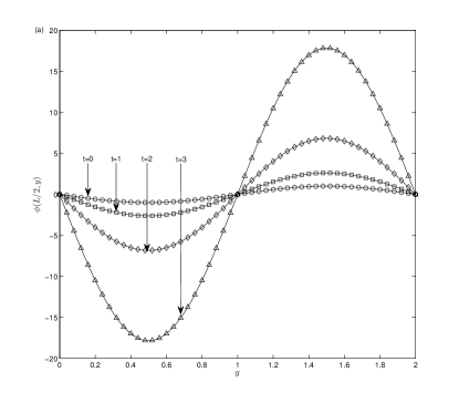
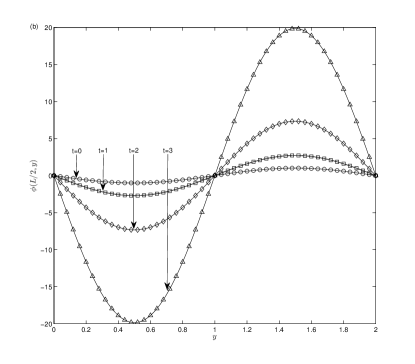
Figure 1: Profiles of scalar variable $\phi$ at different time and Péclet numbers [(a): Pe=100, (b): Pe=1000; solid lines: analytical solutions, symbols: numerical results].

Besides, this problem is also applied to test the convergence rate of the present model since the boundary effect can be eliminated by the periodic boundary conditions adopted. To this end, we conducted a number of simulations and computed the $GRE$s under different lattice resolutions. As shown in Fig. 2 where lattice spacing is varied from $L/500$ to $L/100$ and numerical simulations are suspended at time $T=3.0$, it is clear that present MRT model has a second-order convergence rate in space.

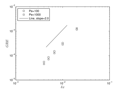
Figure 2: The global relative errors at different lattice sizes ($\delta x=L/500$, $L/400$, $L/300$, $L/200$ and $L/100$), the slope of the inserted line is 2.0, which indicates the present MRT model has a second-order convergence rate in space.

3.2 The two-dimensional Burgers-Fisher equation

The two-dimensional Burgers-Fisher equation, as a special case of the NACDEs, can be written as [35, 46]

$$\partial_{t}\phi+a\phi^{\delta}\partial_{x}\phi=\kappa(\partial_{xx}\phi+\partial_{yy}\phi)+R,$$ (46)

where $R=b\phi(1-\phi^{\delta})$ is the source term, $\delta$, $a$, $b$ and diffusion coefficient $\kappa$ are constants. Compared to the first problem considered above, the present problem is more complicated since it is nonperiodic and nonlinear, but we can still obtain its analytical solution under the proper initial and boundary conditions,

$$\phi(x,y,t)=\{\frac{1}{2}+\frac{1}{2}\tanh[A(x+y-\omega t)]\}^{\frac{1}{\delta}},$$ (47)

where $A$ and $\omega$ are two parameters, and are defined by

$$A=-\frac{a\delta}{4\kappa(\delta+1)},\ \ \omega=\frac{a^{2}+2b\kappa(\delta+1)}{a(\delta+1)}.$$ (48)

Compared with the NACDE defined by Eq. (1), the function $\mathbf{B}(\phi)$ should be given by

$$\mathbf{B}(\phi)=\phi^{\delta+1}(\frac{a}{\delta+1},0)^{\top}.$$ (49)

Based on Eq. (7), one can further derive the tensor $\mathbf{C}$ in Eq. (3),

$$\mathbf{C}=\left({\begin{array}[]{*{20}{c}}\frac{a^{2}}{2\delta+1}\phi^{2\delta+1}&0\\ 0&0\\ \end{array}}\right).$$ (50)

The diffusion tensor $\mathbf{K}$ and tensor $\mathbf{D}$ can be simply determined as

$$\mathbf{K}=\kappa\mathbf{I},\ \ \mathbf{D}=\phi\mathbf{I}.$$ (51)

We now consider how to use present MRT model to solve the Burgers-Fisher equation. If the scheme B is adopted to solve Eq. (46), one needs to use some other methods to solve nonlinear equation (33) since the source term $R$ is a nonlinear function of $\phi$. To avoid such process, the Scheme A is applied to solve the Burgers-Fisher equation. We carried out some simulations in the computational domain $[-1,2]\times[-1,2]$, and presented numerical results and corresponding analytical solutions under different time and different modified Péclet numbers (Pe=$La/\kappa$, $L=3.0$ is the characteristic length) in Fig.3 where the parameters $a$, $b$, and lattice size are fixed to be 4.0, 1.0 and $301\times 301$. As seen from the figure, the numerical results agree well with corresponding analytical solutions.

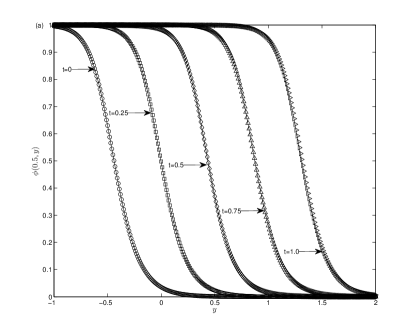
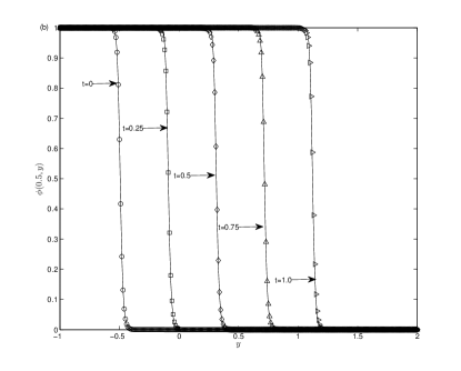
Figure 3: Profiles of the scalar variable $\phi$ at different time and modified Péclet numbers [(a): Pe=100, (b): Pe=1000; solid lines: analytical solutions, symbols: numerical results].

We note that this problem is nonperiodic and the boundary effect cannot be excluded, thus it can be used to test the convergence rate of the MRT model coupling with the non-equilibrium extrapolation scheme. To this end, we also carried out some simulations, and presented the $GRE$s in Fig. 4 where the lattice spacing is ranged from $L/900$ to $L/300$ and simulations are suspended at time $T=1.0$. As shown in this figure, the present MRT model coupling with non-equilibrium extrapolation scheme also has a second-order convergence rate in space. Besides, it is also found that the $GREs$ at Pe=600 is less than those at Pe=120, this may be because the relaxation parameters ($s_{3}$ and $s_{5}$) corresponding to the case of Pe=600 are more close to 1, which usually give more accurate results.

Figure 4: The global relative errors at different lattice sizes ($\delta x=L/900$, $L/750$, $L/600$, $L/450$ and $L/300$), the slope of the inserted line is 2.0, indicating that the present MRT model has a second-order convergence rate in space.

3.3 The two-dimensional Buckley-Leverett equation

We also consider the two-dimensional Buckley-Leverett equation [36, 47, 48]

$$\partial_{t}\phi+\partial_{x}f(\phi)+\partial_{y}g(\phi)=\kappa(\partial_{xx}\phi+\partial_{yy}\phi),$$ (52)

with the following initial condition,

$$\phi(x,y,0)=\left\{\begin{array}[]{ll}1,&x^{2}+y^{2}<0.5,\\ 0,&x^{2}+y^{2}\geq 0.5,\end{array}\\ \right.$$

where $\kappa$ is the diffusion coefficient. $f(\phi)$ and $g(\phi)$ are a function of $\phi$, and are defined as

$$f(\phi)=\frac{\phi^{2}}{\phi^{2}+(1-\phi)^{2}},\ \ \ g(\phi)=f(\phi)[1-5(1-\phi)^{2}].$$ (53)

We note that, similar to the Burgers-Fisher equation considered previously, the Buckley-Leverett equation is also a special NACDE, but there is no analytical solution to this problem.

When the present MRT model is used to solve the problem, the evolution equation [Eq. (2)] can be written more simply since there is no source term included in the the Buckley-Leverett equation,

$$\phi_{k}(\mathbf{x}+\mathbf{c}_{k}\delta t,\;t+\delta t)=\phi_{k}(\mathbf{x},\;t)-(\mathbf{M}^{-1}\mathbf{SM})_{kj}[\phi_{j}(\mathbf{x},\;t)-\phi_{j}^{(eq)}(\mathbf{x},\;t)],$$ (54)

then from Eqs. (1) and (7), one can further determine the functions $\mathbf{B}$, $\mathbf{C}$, $\mathbf{D}$ and diffusion tensor $\mathbf{K}$,

$$\mathbf{B}=[f(\phi),g(\phi)]^{\top},\ \ \mathbf{C}=\left({\begin{array}[]{*{20}{c}}C_{xx}&C_{xy}\\ C_{yx}&C_{yy}\\ \end{array}}\right),\ \ \mathbf{D}=\phi\mathbf{I},\ \ \mathbf{K}=\kappa\mathbf{I},$$ (55)

where the elements of the matrix $\mathbf{C}$ are given as

$$C_{xx}=\frac{1}{2}\arctan(2\phi-1)+\frac{1}{6A^{3}}(2-A+3A^{2})(\phi-\frac{1}{2}),$$ (56a)

$$C_{xy}=C_{yx} = \frac{1}{2}\arctan(2\phi-1)+\frac{5}{4}\ln(\frac{A}{2})$$ (56b)

$$+ \frac{1}{2A}(2+\phi)+\frac{1}{12A^{2}}(\frac{17-4\phi}{2}+\frac{-7+4\phi}{A}),$$

$$C_{yy} = -\frac{17}{8}\arctan(2\phi-1)+\frac{5}{2}\ln(\frac{A}{2})+25\phi[\frac{1}{4}-\frac{\phi}{2}+\frac{\phi^{2}}{3}]$$ (56c)

$$+ \frac{1}{16A}(-89+258\phi)+\frac{1}{16A^{2}}(13+14\phi)+\frac{1}{24A^{3}}(1-42\phi).$$

In our simulations, the computational domain of the problem and the lattice size are set to be $[-1.5,1.5]\times[-1.5,1.5]$ and $301\times 301$. We performed simulations at two different diffusion coefficients ($\kappa=0.1$ and $0.01$) or equivalently two different Péclet numbers (Pe=$LU/\kappa$=30 and 300, $L=3.0$ is the characteristic length, $U=1.0$ is the characteristic velocity), and presented the results at time $T=0.5$ in Figs. 5 and 6. As expected, when the Pe is smaller or the diffusion coefficient is larger, the role of the diffusion becomes dominant, and thus the distribution of scalar variable $\phi$ is more smooth [see Fig. 6(a)]. Besides, to show more details on the distributions of scalar variable $\phi$ at different time, we also conducted some simulations, and presented the results of $\phi$ along the vertical centreline in Fig. 7. As seen from the figure, with the increase of time, the distribution of the scalar variable with a small Pe becomes more smooth.

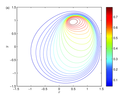
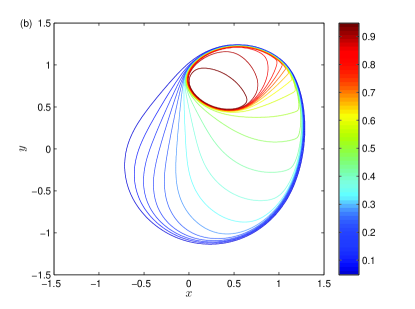
Figure 5: Contours of the scalar variable $\phi$ at the time $T=0.5$ and different Péclet numbers [(a): Pe=30, (b): Pe=300].

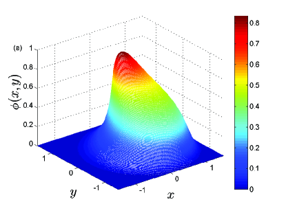
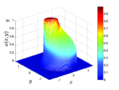
Figure 6: Distributions of the scalar variable $\phi$ at the time $T=0.5$ and different Péclet numbers [(a): Pe=30, (b): Pe=300].

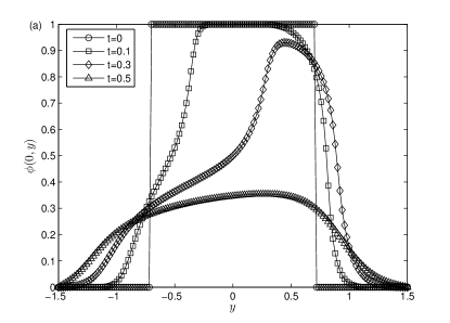
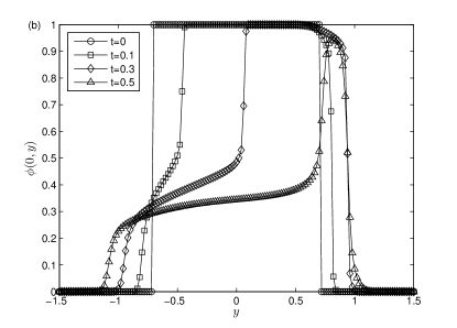
Figure 7: Profiles of the scalar variable $\phi$ at different time and Péclet numbers [(a): Pe=30, (b): Pe=300].

We note that although the problem has no analytical solution, the present results [see Figs. 5(b) and 6(b) where $\kappa=0.01$] agree well with those reported in some previous studies [36, 47, 48], which can also be used to conclude that the present MRT model is also accurate in solving the Buckley-Leverett equation.

3.4 Anisotropic convection-diffusion equation with constant velocity and diffusion tensor

We now consider the problem of the Gaussian hill with constant velocity and diffusion tensor, which is also a classic benchmark example and has also been used to validate LB models for anisotropic CDEs [27, 30, 32, 34]. The CDE for this problem can be written as

$$\partial_{t}\phi+\nabla\cdot(\phi\mathbf{u})=\nabla\cdot(\mathbf{K}\cdot\nabla\phi),$$ (57)

where $\mathbf{u}=(u_{x},u_{y})^{\top}$ is a constant velocity, $\mathbf{K}$ is the constant diffusion tensor, and can be defined as

$$\mathbf{K}=\left({\begin{array}[]{*{20}{c}}\kappa_{xx}&\kappa_{xy}\\ \kappa_{yx}&\kappa_{yy}\\ \end{array}}\right).$$ (58)

Under the proper initial and boundary conditions, one can also derive the analytical solution of the problem,

$$\phi(x,y,t)=\frac{\phi_{0}}{2\pi|\det(\sigma)|^{1/2}}\exp\{-\frac{\sigma^{-1}:[(\mathbf{x}-\mathbf{u}t)(\mathbf{x}-\mathbf{u}t)]}{2}\},$$ (59)

where $\mathbf{x}=(x,y)^{\top}$, $\sigma=\sigma_{0}^{2}\mathbf{I}+2\mathbf{K}t$, $\sigma^{-1}$ is inverse matrix of $\sigma$, $|\det(\sigma)|$ is the absolute value of the determinant of $\sigma$.

Actually, there are two approaches that can be adopted to study the Gaussian hill problem. The first is that we directly use the MRT model to solve Eq. (57) with an anisotropic form, and set the functions $\mathbf{B}$, $\mathbf{C}$, and $\mathbf{D}$ as

$$\mathbf{B}=(\phi u_{x},\phi u_{y})^{\top},\ \ \mathbf{C}=\left({\begin{array}[]{*{20}{c}}\phi u_{x}^{2}&\phi u_{x}u_{y}\\ \phi u_{x}u_{y}&\phi u_{y}^{2}\\ \end{array}}\right),\ \ \mathbf{D}=\phi\mathbf{I}.$$ (60)

While in the second approach, we first need to write Eq. (57) in an isotropic form,

$$\partial_{t}\phi+\nabla\cdot(\phi\mathbf{u})=\nabla\cdot[\kappa(\nabla\cdot\mathbf{D})].$$ (61)

which is then solved by the MRT model. In addition, it should be noted that Eq. (61) can also be solved by the previous BGK model [35]. Based on Eq. (61), one can also find that the functions $\mathbf{B}$ and $\mathbf{C}$ should be the same as those appeared in Eq. (60), but the tensor $\mathbf{D}$ should be given by $\mathbf{D}=\mathbf{K}\phi/\kappa$ with $\kappa$ being a positive constant.

Similar to some previous works [32, 34], we also considered the Gaussian hill problem in a bounded domain $[-1,1]\times[-1,1]$, and adopted the periodic boundary condition on all boundaries. In our simulations, $\sigma_{0}=0.01$ which is small enough to ensure that the periodic boundary condition adopted is reasonable and accurate at a finite time $T$, $\phi_{0}=2\pi\sigma_{0}^{2}$, $u_{x}=u_{y}=0.01$, and the lattice size is $401\times 401$. To test the capacity of the present MRT model in solving the anisotropic CDEs, the following three types of diffusion tensor are considered,

$$\mathbf{K}=\left[\left({\begin{array}[]{*{20}{c}}1&0\\ 0&1\\ \end{array}}\right),\ \ \left({\begin{array}[]{*{20}{c}}1&0\\ 0&2\\ \end{array}}\right),\ \ \left({\begin{array}[]{*{20}{c}}1&1\\ 1&2\\ \end{array}}\right)\right]\times 10^{-3},$$ (62)

which are usually denoted as isotropic, diagonally anisotropic and fully anisotropic diffusion problems.

We conducted some simulations by using above two approaches, and presented numerical results in Figs. 8, 9 and 10 where $\kappa=10^{-3}$ is used in the second approach. As seen from these figures, the numerical results qualitatively agree with analytical solutions. To quantitatively measure the deviations between numerical results and analytical solutions, the $GRE$s of isotropic, diagonally anisotropic and fully anisotropic diffusion problems are computed, and the values of them are $1.199\times 10^{-4}$, $3.853\times 10^{-4}$ and $6.531\times 10^{-4}$ for the first approach, while they are $1.199\times 10^{-4}$, $2.118\times 10^{-4}$ and $4.572\times 10^{-4}$ for the second approach, which illustrate that the present MRT model is accurate in studying these problems. Besides, the convergence rate of the MRT model for anisotropic CDEs is also investigated, and the results are shown in Fig. 11 where the lattice size is varied from $201\times 201$ to $801\times 801$. From this figure, one can find that, similar to some available MRT models for anisotropic diffusion problems [32, 34], the present MRT model also has a second-order convergence rate in space.

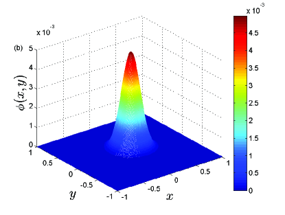
Figure 8: Distributions of the scalar variable $\phi$ at the time $T=10$ [Isotropic diffusion problem: numerical solution (a), analytical solution (b)].

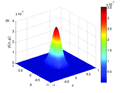
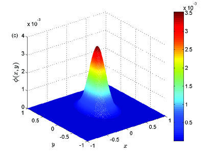
Figure 9: Distributions of the scalar variable $\phi$ at the time $T=10$ [Diagonally anisotropic diffusion problem: first approach (a), second approach (b), analytical solution (c)].

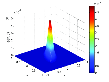
Figure 10: Distributions of the scalar variable $\phi$ at the time $T=10$ [Fully anisotropic diffusion problem: first approach (a), second approach (b), analytical solution (c)].

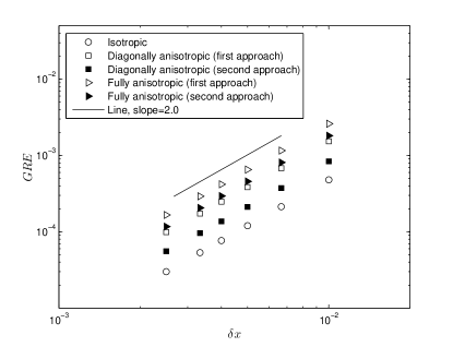
Figure 11: The global relative errors at different lattice sizes ($\delta x=L/800$, $L/600$, $L/500$, $L/400$, $L/300$ and $L/200$, $L=2.0$ is the characteristic length), the slope of the inserted line is 2.0, which indicates that the present MRT model has a second-order convergence rate in space.

3.5 Anisotropic convection-diffusion equation with constant velocity and variable diffusion tensor

In this part, we will consider the following anisotropic CDE with a constant velocity $\mathbf{u}=(u_{x},u_{y})^{\top}$ and a variable diffusion tensor $\mathbf{K}$,

$$\partial_{t}\phi+\nabla\cdot(\phi\mathbf{u})=\nabla\cdot(\mathbf{K}\cdot\nabla\phi)+R.$$ (63)

where $R$ is the source term. We note that the problem is more complicated since the diffusion tensor $\mathbf{K}$ is a function of space $\mathbf{x}$. For this reason, we cannot write Eq. (63) in an isotropic form, and thus the problem cannot be solved directly by the previous BGK model [35].

In this work, the diffusion tensor $\mathbf{K}$ is simply given by a diagonal matrix,

$$\mathbf{K}=\kappa\left({\begin{array}[]{*{20}{c}}2-\sin(2\pi x)\sin(2\pi y)&0\\ 0&1\\ \end{array}}\right),$$ (64)

where $\kappa$ is a constant, and is fixed to be $1.0\times 10^{-3}$. The source term $R$ is defined as

$$R = \exp[(1-12\pi^{2}\kappa)t]\{\sin(2\pi x)\sin(2\pi y)+4\kappa\pi^{2}\cos(4\pi x)\sin^{2}(2\pi y)$$ (65)

$$+ 2\pi[u_{x}\cos(2\pi x)\sin(2\pi y)+u_{y}\sin(2\pi x)\cos(2\pi y)]\}.$$

Under the periodic boundary conditions on the physical region $[0,1]\times[0,1]$ and the following initial condition,

$$\phi(x,y,t=0)=\sin(2\pi x)\sin(2\pi y),$$ (66)

one can derive the exact solution of the problem,

$$\phi=\exp[(1-12\pi^{2}\kappa)t]\sin(2\pi x)\sin(2\pi y).$$ (67)

Based on Eq. (63), one can determine the functions $\mathbf{B}$, $\mathbf{C}$ and $\mathbf{D}$, which are the same as those appeared in Eq. (60). We now performed some simulations with a fixed lattice size $401\times 401$, and presented the results at time $T=3.0$ and different Péclet numbers (Pe=$Lu_{x}/\kappa$, $L=1.0$ is the characteristic length, $u_{x}=u_{y}=0.1$ is the characteristic velocity) in Figs. 12 and 13 where Pe=100 and 1000. As seen from these figures, the numerical results are very close to the analytical solutions. To quantitatively measure the deviations between numerical results and corresponding analytical solutions, we also computed the $GRE$s of these two cases, and found that the values of them are $6.207\times 10^{-4}$ and $9.831\times 10^{-5}$, which are small enough and can be used to demonstrate that the present MRT model is accurate in the study of the anisotropic CDE with a variable diffusion tensor.

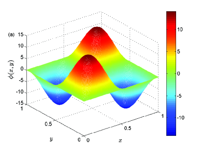
Figure 12: Distributions of the scalar variable $\phi$ at the time $T=3$ and Pe=100 [(a): numerical solution, (b): analytical solution].

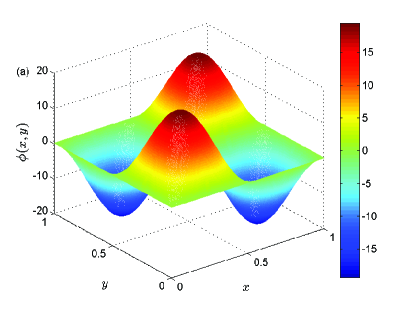
Figure 13: Distributions of the scalar variable $\phi$ at the time $T=3$ and Pe=1000 [(a): numerical solution, (b): analytical solution].

To show the convergence rate of the present MRT for such complicated problem, we also carried out a number of simulations under different lattice resolutions, and presented the results in Fig. 14 where the lattice size is varied from $201\times 201$ to $801\times 801$. As shown in this figure, the present MRT model also has a second-order convergence rate for this special problem.

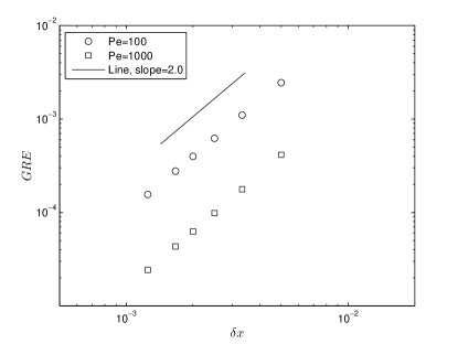
Figure 14: The global relative errors at different lattice sizes ($\delta x=L/800$, $L/600$, $L/500$, $L/400$, $L/300$ and $L/200$), the slope of the inserted line is 2.0, indicating that the present MRT model has a second-order convergence rate in space.

3.6 A comparison between the MRT model and BGK model

As reported in some available works [4, 30, 22, 32, 34], through tuning the relaxation parameters properly, the MRT model could be more accurate and more stable than the BGK model. To show the superiority of the MRT model over the BGK model, a comparison between two models is also conducted.

We first performed a comparison of accuracy between the BGK model and MRT model through adopting a simple problem defined in a physical region $[0,L]\times[0,L]$, which can be described by the following CDE and boundary conditions,

$$\partial_{t}\phi+\nabla\cdot(\phi\mathbf{u})=\nabla\cdot(\kappa\nabla\phi)+R,$$ (68a)

$$\phi(t,x,0)=\phi_{0},\phi(t,x,L)=\phi_{L},$$ (68b)

where $\kappa$ is a constant diffusion coefficient, $\mathbf{u}=(u_{x},u_{y})^{\top}$ is a constant velocity with $u_{y}=0$, $\phi_{0}$ and $\phi_{L}$ are two constants, $R=2\kappa\Delta\phi/L^{2}$ is the source term with $\Delta\phi=\phi_{L}-\phi_{0}$. Under an assumption that the problem is steady and unidirectional, i.e., $\phi$ is only a function of $y$, we can derive analytical solution of the problem,

$$\phi(y)=\phi_{0}+\Delta\phi\frac{y}{L}(2-\frac{y}{L}).$$ (69)

The reason for choosing this problem is that, following a similar procedure reported in Ref. [49], one can readily derive the analytical solutions of the BGK model and MRT model (Scheme B with $s_{1}=s_{2}=s_{4}=s_{6}=s_{7}=s_{8}$) with adopting the anti-bounce back boundary condition [28, 50, 22],

$$\phi_{j}=\phi_{0}-\Delta\phi\bar{y}_{j}(2.0-\bar{y}_{j})+\phi_{s},$$ (70)

where $\bar{y}_{j}=(j-1/2)/N$ with $N$ representing the grid number used in $y$ direction, $\phi_{s}$ is numerical slip caused by the model adopted, and can be given by

$$\phi_{s,BGK}=\frac{\Delta\phi}{12N^{2}}[4(\frac{2}{s_{BGK}}-1)^{2}-3],$$ (71a)

$$\phi_{s,MRT}=\frac{\Delta\phi}{12N^{2}s_{1}s_{3}}[s_{1}s_{3}-8(s_{1}+s_{3})+16].$$ (71b)

Based on Eq. (71a), one can find that although the BGK model has a second-order convergence rate for this simple problem, the numerical slip of the scalar variable $\phi$ cannot be eliminated unless $s_{BGK}=4(2-\sqrt{3})$. While for the MRT model, we can make the solution of MRT model [Eq. (71b)] consistent with that of the physical problem [Eq. (69)] through setting $\phi_{s}$ to be zero, which means that the relaxation parameters $s_{1}$ and $s_{3}$ should satisfy the following relation,

$$s_{1}=\frac{8(s_{3}-2)}{8-s_{3}}.$$ (72)

From above theoretical analysis, it is clear that the MRT model can be more accurate than the BGK model through tuning the free relaxation parameter $s_{1}$. In addition, similar to the procedure used in above examples, the functions $\mathbf{B}$, $\mathbf{C}$ and $\mathbf{D}$, the diffusion tensor $\mathbf{K}$, and the source term $R_{i}$ used in our model can also be determined,

$$\mathbf{B}=\phi\mathbf{u},\ \ \mathbf{C}=\phi\mathbf{u}\mathbf{u},\ \ \mathbf{D}=\phi\mathbf{I},\ \ \mathbf{K}=\kappa\mathbf{I},\ \ R_{i}=\omega_{i}(1+\frac{\mathbf{c}_{i}\cdot\mathbf{u}}{c_{s}^{2}})R.$$ (73)

To validate above analysis and confirm our statement, we also performed some simulations with different lattice resolutions and relaxation parameters ($s_{3}$), and presented the results in Fig. 15 where $L=1.0$, $u_{x}=0.1$, $\phi_{0}=0$, $\phi_{L}=1.0$, and the diffusion coefficient $\kappa$ is set to be 0.1. As seen from Fig. 15, the numerical results obtained by the MRT model are in good agreement with the analytical solution [Eq. 69] even with a coarse grid (e.g., $N=4$), while the results given by the BGK model deviate from the analytical solution unless the relaxation parameter $s_{BGK}$ is fixed to be $s_{3}=4(2-\sqrt{3})$, which is consistent with above theoretical analysis.

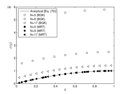
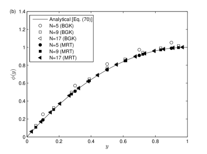
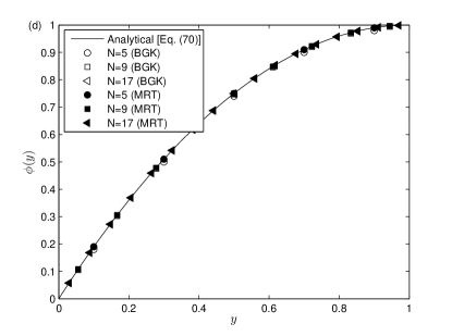
Figure 15: Comparisons between the BGK model and MRT model under different lattice sizes and relaxation parameters [(a): $s_{3}=0.1$, (b): $s_{3}=0.6$, (c): $s_{3}=4(2-\sqrt{3})$, (d): $s_{3}=1.9$].

Then a comparison of stability between the BGK model and MRT model is also carried out through using the Gaussian hill problem, which has been investigated previously. Here we only take the fully anisotropic diffusion problem as an example, while to simply perform a comparison between the BGK and MRT models, the second approach presented in section 3.4 [the anisotropic CDE is written in an isotropic form, see Eq. (61)] is adopted. In the following simulations, the diffusion tensor $\mathbf{K}$ is taken as

$$\mathbf{K}=\kappa\left({\begin{array}[]{*{20}{c}}1&1\\ 1&2\\ \end{array}}\right),$$ (74)

from which one can further determine the function $\mathbf{D}=\mathbf{K}\phi/\kappa$ in the second approach [see Eq. (60)]. $\kappa$ is a constant, and is varied to test the stability of the BGK model and MRT model. The lattice speed $c$ is equal to 1.0, the velocity $\mathbf{u}$ is fixed to be $\mathbf{u}=(0.1,0.1)^{\top}$. For the relaxation parameters appeared in the MRT model, $s_{3}$ and $s_{5}$ can be determined from $\kappa$, and the others are fixed through the following equation,

$$s_{0}=0,\ s_{1}=s_{2}=s_{4}=s_{6}=s_{7}=s_{8}=s,$$ (75)

where $s$ can be varied in a proper range to ensure that the MRT model is stable, but for simplicity, only a special case $s=0.6$ is considered. The other parameters used in simulations are the same as those appeared in section 3.4 except for time $T=5.0$.

We first conducted simulations with $\kappa=10^{-3}$, and presented the results in Fig.16. As shown in this figure, both numerical results obtained by the BGK model and MRT model are close to the analytical solution. However, when $\kappa$ is decreased to $10^{-4}$, the BGK model is unstable, while the MRT model can give a stable solution (see Fig. 17), and the $GRE$ is about $4.438\times 10^{-2}$.

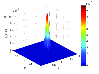
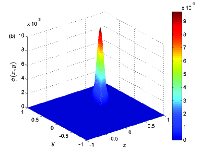
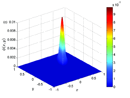
Figure 16: A comparison between the BGK model and MRT model for fully anisotropic diffusion problem ($\kappa=10^{-3}$) [(a): BGK model, (b): MRT model, (c): Analytical solution].

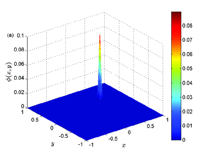
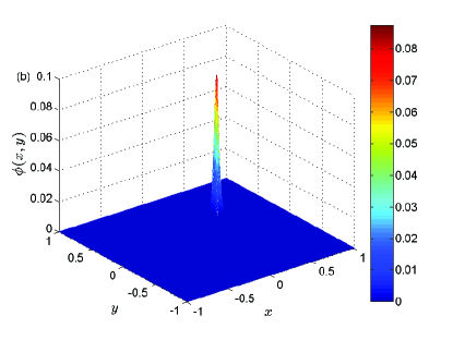
Figure 17: A comparison between the BGK model and MRT model for fully anisotropic diffusion problem ($\kappa=10^{-4}$) [(a): MRT model, (b): Analytical solution].

From above discussion, it is clear that, through tuning the relaxation parameters properly, the MRT could be more accurate and more stable than the BGK model.

4 Conclusions

In this work, a general multiple-relaxation-time lattice Boltzmann model for nonlinear anisotropic convection-diffusion equations is proposed, and is then tested by some classic NACDEs, including the simple linear CDE, nonlinear Burgers-Fisher equation, nonlinear Buckley-Leverett equation and some anisotropic CDEs. The numerical results show that the present MRT model is efficient and accurate in solving the NACDEs, and also has a second-order convergence rate in space. Besides, we also conducted a comparison between the BGK model and MRT model, and found that the present MRT model could be more accurate and more stable than BGK model through tuning the relaxation parameters properly. And finally, we would also like to point out that, based on the superiority of the MRT model and the role of the NACDEs in describing the physical phenomena caused by the convection and diffusion processes, the present work may promote the MRT model in the study of heat and mass transfer [2, 4], multiphase flows and crystal growth based on phase-field models [15, 23, 51].

References

- [1] S. Chen and G. Doolen, Lattice Boltzmann method for fluid flows, Annu. Rev. Fluid Mech. 30 (1998) 329-364.
- [2] S. Succi, The Lattice Boltzmann Equation for Fluid Dynamics and Beyond (Clarendon Press, Oxford, 2001).
- [3] C. K. Aidun and J. R. Clausen, Lattice Boltzmann method for complex flows, Annu. Rev. Fluid Mech. 42 (2010) 439-471.
- [4] Z. Guo and C. Shu, Lattice Boltzmann Method and Its Applications in Engineering (World Scientific, Singapore, 2013).
- [5] D. Wolf-Gladrow, A lattice Boltzmann equation for diffusion, J. Statist. Phys. 79 (1995) 1023-1032.
- [6] C. Huber, B. Chopard, M. Manga, A lattice Boltzmann model for coupled diffusion, J. Comput. Phys. 229 (2010) 7956-7976.
- [7] G. Yan, A lattice Boltzmann equation for waves, J. Comput. Phys. 161 (2000) 61-69.
- [8] X. M. Yu and B. C. Shi, A lattice Bhatnagar-Gross-Krook model for a class of the generalized Burgers equations, Chinese Phys. 15 (2006) 1441-1449.
- [9] Z. Chai and B. Shi, A novel lattice Boltzmann model for the Poisson equation, Appl. Math. Model. 32 (2008) 2050-2058.
- [10] S. P. Dawson, S. Chen, G. D. Doolen, Lattice Boltzmann computations for reaction-diffusion equations, J. Chem. Phys. 98 (1993) 1514-1523.
- [11] Z. L. Guo, B. C. Shi, N. C. Wang, Fully lagrangian and lattice Boltzmann methods for the advection-diffusion equation, J. Sci. Comput. 14 (1999) 291-300.
- [12] R. G. M. van der Sman and M. H. Ernst, Convection-diffusion lattice Boltzmann scheme for irregular lattices, J. Comput. Phys. 160 (2000) 766-782.
- [13] X. He N. Li, B. Goldstein, Lattice Boltzmann simulation of diffusion-convection systems with surface chemical reaction, Mol. Simulat. 25 (2000) 145-156.
- [14] B. Deng, B. C. Shi, G. C. Wang, A new lattice Bhatnagar-Gross-Krook Model for the convection-diffusion equation with a source term, Chin. Phys. Lett. 22 (2005) 267-270.
- [15] H. W. Zheng, C. Shu, Y. T. Chew, A lattice Boltzmann model for multiphase flows with large density ratio, J. Comput. Phys. 218 (2006) 353-371.
- [16] B. C. Shi, B. Deng, R. Du, X. W. Chen, A new scheme for source term in LBGK model for convection-diffusion equation, Comput. Math. Appl. 55 (2008) 1568-1575.
- [17] B. Chopard, J. L. Falcone, J. Latt, The lattice Boltzmann advection-diffusion model revisited, Eur. Phys. J. Special Topics 171 (2009) 245-249.
- [18] H.-B. Huang, X.-Y. Lu, M. C. Sukop, Numerical study of lattice Boltzmann methods for a convection-diffusion equation coupled with Navier-Stokes equations, J. Phys. A 44 (2011) 055001.
- [19] Z. Chai and T. S. Zhao, Lattice Boltzmann model for the convection-diffusion equation, Phys. Rev. E 87 (2013) 063309.
- [20] J. Perko and R. A. Patel, Single-relaxation-time lattice Boltzmann scheme for advection-diffusion problems with large diffusion-coefficient heterogentities and high-advection transport, Phys. Rev. E 89 (2014) 053309.
- [21] H. Yoshida and M. Nagaoka, Lattice Boltzmann method for the convection-diffusion equation in curvilinear coordinate systems, J. Comput. Phys. 257 (2014) 884-900.
- [22] Z. Chai and T. S. Zhao, Nonequilibrium scheme for computing the flux of the convection-diffusion equation in the framework of the lattice Boltzmann method, Phys. Rev. E 90 (2014) 013305.
- [23] H. Liang, B. C. Shi, Z. L. Guo, and Z. H. Chai, Phase-field-based multiple-relaxation-time lattice Boltzmann model for incompressible multiphase flows, Phys. Rev. E, 89 (2014) 053320.
- [24] R. Huang and H. Wu, Lattice Boltzmann model for the correct convection-diffusion equation with divergence-free velocity field, Phys. Rev. E, 91 (2015) 033302.
- [25] X. Zhang, A. G. Bengough, J. W. Crawford, I. M. Young, A lattice BGK model for advection and anisotropic dispersion equation, Adv. Water Resour. 25 (2002) 1-8.
- [26] S. Suga, Stability and accuracy of lattice Boltzmann schemes for anisotropic advection-diffusion equations, Int. J. Mod. Phys. C 20 (2009) 633-650.
- [27] I. Ginzburg, Equilibrium-type and link-type lattice Boltzmann models for generic advection and anisotropic-dispersion equation, Adv. Water Resour. 28 (2005) 1171-1195.
- [28] I. Ginzburg, Generic boundary conditions for lattice Boltzmann models and their application to advection and anisotropic dispersion equations, Adv. Water Resour. 28 (2005) 1196-1216.
- [29] I. Ginzburg, Truncation Errors, exact and heuristic stability analysis of two-relaxation-times lattice Boltzmann schemes for anisotropic advection-diffusion equation, Commun. Comput. Phys. 11 (2012) 1439-1502.
- [30] B. Servan-Camas, F. T.-C. Tsai, Lattice Boltzmann method with two relaxation times for advection-diffusion equation: Third order analysis and stability analysis, Adv. Water Resour. 31 (2008) 1113-1126.
- [31] I. Rasin, S. Succi, W. Miller, A multi-relaxation lattice kinetic method for passive scalar diffusion, J. Comput. Phys. 206 (2005) 453-462.
- [32] H. Yoshida and M. Nagaoka, Multiple-relaxation-time lattice Boltzmann model for the convection and anisotropic diffusion equation, J. Comput. Phys. 229 (2010) 7774-7795.
- [33] L. Li, R. Mei, J. F. Klausner, Multiple-relaxation-time lattice Boltzmann model for the axisymmetric convection diffusion equation, Int. J. Heat Mass Transfer 67 (2013) 338-351.
- [34] R. Huang, H. Wu, A modified multiple-relaxation-time lattice Boltzmann model for convection-diffusion equation, J. Comput. Phys. 274 (2014) 50-63.
- [35] B. Shi and Z. Guo, Lattice Boltzmann model for nonlinear convection-diffusion equations, Phys. Rev. E 79 (2009) 016701.
- [36] B. Shi and Z. Guo, Lattice Boltzmann simulation of some nonlinear convection-diffusion equations, Comput. Math. Appl. 61 (2011) 3443-3452.
- [37] P. Lallemand and L. S. Luo, Theory of the lattice Boltzmann method: Dispersion, dissipation, isotropy, Galilean invariance, and stability, Phys. Rev. E 61 (2000) 6546-6562.
- [38] Y. H. Qian, D. d’Humières, and P. Lallemand, Lattice BGK models for Navier-Stokes equation, Europhys. Lett. 17 (1992) 479-484.
- [39] S. Ansumali, I. V. Karlin, and H. C. Öttinger, Minimal entropic kinetic models for hydrodynamics, Europhys. Lett. 63 (2003) 798-804.
- [40] I. Ginzburg, F. Verhaeghe, and D. d’Humières, Two-relaxation-time lattice Boltzmann scheme: About parametrization, velocity, pressure and mixed boundary conditions, Commun. Comput. Phys. 3 (2008) 427-478.
- [41] D. d’Humières, Generalized lattice-Boltzmann equations, in: B.D. Shizgal, D.P. Weave (Eds.), Rarefied Gas Dynamics: Theory and Simulations, in: Prog. Astronaut. Aeronaut., Vol. 159, AIAA, Washington, DC, 1992, pp. 450-458.
- [42] L.-S. Luo, W. Liao, X. Chen, Y. Peng, and W. Zhang, Numerics of the lattice Boltzmann method: Effects of collision models on the lattice Boltzmann simulations, Phys. Rev. E 83 (2011) 056710.
- [43] Z. Chai and T. S. Chai, Effect of the forcing term in the multiple-relaxation-time lattice Boltzmann equation on the shear stress or the strain rate tensor, Phys. Rev. E 86 (2012) 016705.
- [44] X. He, S. Chen, and G. D. Doolen, A novel thermal model for the lattice Boltzmann method in incompressible limit, J. Comput. Phys. 146 (1998) 282-300.
- [45] Z.-L. Guo, C.-G. Zheng, and B.-C. Shi, Non-equilibrium extrapolation method for velocity and pressure boundary conditions in the lattice Boltzmann method, Chinese Phys. 11 (2002) 366-374.
- [46] A.-M. Wazwaz, The tanh method for generalized forms of nonliner heat conduction and Burgers-Fisher equations, Appl. Math. Comput. 169 (2005) 321-338.
- [47] K. H. Karlsen, K. Brusdal, H. K. Dahle, S. Evje, and K.-A. Lie, The corrected operator splitting approach applied to a nonlinear advection-diffusion problem, Comput. Methods Appl. Mech. Engrg. 167 (1998) 239-260.
- [48] A. Kurganov and E. Tadmor, New high-resolution central schemes for nonlinear conservation laws and convection-diffusion equations, J. Comput. Phys. 160 (2000) 241-282.
- [49] X. He, Q. Zou, L.-S. Luo, and M. Dembo, Analytic solutions and analysis on non-slip boundary condition for the lattice Boltzmann BGK model, J. Stat. Phys. 87 (1997) 115-136.
- [50] T. Zhang, B. Shi, Z. Guo, Z. Chai, and J. Lu, General bounce-back scheme for concentration boundary condition in the lattice-Boltzmann method, Phys. Rev. E 85 (2012) 016701.
- [51] W. J. Boettinger, J. A. Warren, C. Beckermann, and A. Karma, Phase-field simualtion of solidification, Annu. Rev. Mater. Res. 32 (2002) 163-194.