First-principles approach to the dynamic magnetoelectric couplings in BiFeO₃

Abstract

Despite its great technological importance, the magnetoelectric (ME) couplings in BiFeO₃ are barely understood. By using a first-principles approach, we uncover the dynamic ME couplings of the long-range spin-cycloid in BiFeO₃. Based on a microscopic Hamiltonian, our first-principles approach disentangles the hidden ME couplings due to spin-current and exchange-striction. Beyond the spin-current polarization governed by the inverse Dzyaloshinskii-Moriya interaction iDM , various spin-current polarizations derived from both ferroelectric and antiferrodistortive distortions cooperatively produce the strong non-reciprocal directional dichroism or the asymmetry in the absorption of counter-propagating light in BiFeO₃. Our systematic approach can be generally applied to any multiferroic material, laying the foundation for revealing hidden ME couplings on an atomic scale and for exploiting optical ME effects in the next generation of technological devices such as optical diodes.

The heroic characteristics of BiFeO₃ , i.e. its room-temperature ferroelectric ($T_{\rm C}\approx$ 1100 K teague70 ) and magnetic ($T_{\rm N}\approx$ 640 K sosnowska82 ) transitions and large ferroelectric polarization lebeugle07 below $T_{\rm C}$, have unexpectedly hampered our understanding of the magneto-capacitance effects driven by spin ordering below $T_{\rm N}$. Because BiFeO₃ is a type-$I$ multiferroic, its spin-driven polarizations and magnetoelectric (ME) behavior are veiled by a large preexisting FE polarization. Despite a great deal of effort kadomtseva04 ; tokunaga10 ; park11 ; sosnowska82 ; lebeugle08 ; rama11a ; sosnowska11 and the strong ME effects revealed by recent neutron-scattering lee13 and Raman-spectroscopy rov10 measurements, little is known about the microscopic origins of the spin-driven polarizations and ME couplings in BiFeO₃.

Due to the lack of spatial inversion and time reversal symmetries in multiferroics, the intimate coupling between spins and local electric dipoles can give rise to strong ME effects fiebig05 . Such ME effects, mostly studied in the static limit so far, can resonantly be enhanced at the so-called ME spin-wave excitations characterized by a coupled dynamics of spins and local electric dipoles fiebig05 . Non-reciprocal directional dichroism (NDD) or the difference in the absorption of counter-propagating light beams has proven to be a powerful tool to investigate intrinsic ME couplings in several multiferroics kezsmarki11 ; takahashi12 ; bordacs12 ; miy12 ; szaller13 .

BiFeO₃ has two distinctive structural distortions that eliminate inversion centers and can couple to the electric component of light. One is the ferroelectric (FE) distortion ($\Gamma_{4}^{-}$[111]), which breaks global inversion-symmetry (IS), and the other is the antiferrodistortive (AFD) octahedral rotation ($R_{4}^{+}$[111]), which breaks the local IS between nearest neighbor spins.

Using a first-principles approach based on a microscopic Hamiltonian, we show that all ME couplings are microscopically driven by a distinctive combination of these two inherent structural distortions. Four spin-current polarizations associated with the FE and AFD distortions cooperatively induce the strong NDD in BiFeO₃. This type of study of dynamical or optical ME effects is especially powerful for leaky ferroelectrics where static magneto-capacitance measurements are not feasible and for type-$I$ multiferroics such as BiFeO₃ where the evaluation of static magneto-capacitance data is not straightforward due to the large preexisting FE polarization of roughly $90\mu$C/cm² [lebeugle07, ].

1. Microscopic spin-cycloid model for R3c BiFeO₃.

The FE and AFD distortions each creates its own Dzyaloshinskii-Moriya (DM) interaction, $\textbf{\emph{D}}_{\rm FE}$ and $\textbf{\emph{D}}_{\rm AFD}$. By including all magnetic anisotropies governed by the FE and AFD distortions, the spin Hamiltonian can be written as

$${\cal H}=\;{\cal H^{\rm SC}_{\rm FE}}\;+\;{\cal H^{\rm SC}_{\rm AFD}}\;+{\cal H^{\rm EX}}+{\cal H^{\rm SIA}}$$ (1)

$${\cal H^{\rm SC}_{\rm FE}}=\sum_{\langle i,j\rangle}\textbf{\emph{D}}_{\rm FE}\cdot({\bf S}_{i}\times{\bf S}_{j})$$ (2)

$${\cal H^{\rm SC}_{\rm AFD}}=\sum_{\langle i,j\rangle}\,(-1)^{n_{i}}\textbf{\emph{D}}_{\rm AFD}\cdot({\bf S}_{i}\times{\bf S}_{j})$$ (3)

$${\cal H^{\rm EX}}=-J_{1}\sum_{\langle i,j\rangle}{\bf S}_{i}\cdot{\bf S}_{j}-J_{2}\sum_{\langle i,j\rangle^{\prime}}{\bf S}_{i}\cdot{\bf S}_{j}$$ (4)

$${\cal H^{\rm SIA}}=-K\sum_{i}({\bf S}_{i}\cdot{\bf z}^{\prime})^{2},$$ (5)

where $\langle i,j\rangle$ and $\langle i,j\rangle^{\prime}$ represent nearest and next-nearest neighbor spins, respectively. The FE polarization lies along ${\bf z}^{\prime}=[1,1,1]$ (all unit vectors are assumed normalized to one). Since the FE distortion is uniform, its DM interaction ($\textbf{\emph{D}}_{\rm FE}$) is translation-invariant. By contrast, the translation-odd R${}_{4}^{+}$[111] AFD octahedral rotation requires the coefficient $(-1)^{{n_{i}}}$, which alternates from one hexagonal layer $n_{i}$ to the next, in front of $\textbf{\emph{D}}_{\rm AFD}$. The final contribution to the Hamiltonian is the single-ion anisotropy (SIA) proportional to the corresponding coefficient $K$. SIA favors spin alignment along the FE polarization direction ${\bf z}^{\prime}$. Simplified forms for the DM terms $\cal{H}^{\rm SC}_{\rm FE}$ and $\cal{H}^{\rm SC}_{\rm AFD}$ are given in Appendix A.

By ignoring the cycloidal harmonics but including the tilt pyatakov09 $\tau$ produced by $\textbf{\emph{D}}_{\rm AFD}$, the spin state can be approximated fishman13b as

$$S_{x^{\prime}}({\bf R}) = S(-1)^{n+1}\cos\tau\sin(2\pi\delta r),$$ (6)

$$S_{y^{\prime}}({\bf R}) = S\sin\tau\sin(2\pi\delta r),$$ (7)

$$S_{z^{\prime}}({\bf R}) = S(-1)^{n+1}\cos(2\pi\delta r).$$ (8)

We recall that fishman13a $\sin\tau=S_{0}/S$ where $M_{0}=2\,\mu_{\rm B}S_{0}$ is the weak FM moment of the AF phase along ${\bf y}^{\prime}$ above $H_{c}$. For moment tokunaga10 ; weakFM $M_{0}=0.03\,\mu_{\rm B}$, $\tau=0.006$ or 0.34^∘. By comparison, our result of Local Spin-Density Approximation (LSDA)+$U$ ($U=5$ eV) indicates that $M_{0}=0.029\,\mu_{\rm B}$. Because higher harmonics are neglected, averages taken with the tilted cycloid introduce a very small error of order ${C_{3}}^{2}\approx 2.5\times 10^{-5}$.

2. First-principles method

First-principles calculations were performed using density functional theory (DFT) from the VASP code within a local spin-density approximation with an additional Hubbard (LSDA+$U$) interaction for the exchange-correlation functional. The Hubbard $U$ and the exchange $J_{\rm H}$ were set to $U$ = 5 eV and $J_{\rm H}$ = 0 eV for Fe³⁺, parameters that were found to be optimal for BiFeO₃ wein12 ; ed05 . We used the projector augmented wave (PAW) potentials PAW1 ; PAW2 . To integrate over the Brillouin zone, we used a supercell made of a 2$\times$2$\times$2 perovskite units (40 atoms, 8 f.u.), 3$\times$3$\times$3 Monkhorst-Pack (MP) $k$-points mesh. To evaluate $\textbf{\emph{D}}_{\rm FE}$ and $\textbf{\emph{D}}_{\rm AFD}$, we employed a 4$\times$2$\times$2 unit (80 atoms, 16 f.u.) with a 1$\times$3$\times$3 Monkhorst-Pack (MP) mesh. The wave functions were expanded with plane waves up to an energy cutoff of 500 eV. To calculate exchange interactions ($J_{n}$), we used four different magnetic configurations ($G$-AFM, $C$-AFM, $A$-AFM and FM). The DM parameters $\textbf{\emph{D}}_{\rm FE}$ and $\textbf{\emph{D}}_{\rm AFD}$ were estimated by replacing all except for four of Fe³⁺ cations with Al³⁺ wein12 in the 80 atom unit cell.

After obtaining the exchange, DM, aand SIA interactions, we calculated their derivatives with respect to an applied electric field parallel to a cartesian direction. To simulate atomic displacements driven by the applied field ($E_{\alpha}$) in bulk BiFeO₃, we calculated the lowest-frequency polar eigenvector from the dynamical matrix and forcibly move the atoms incrementally from the ground state ($R3c$) structure. The resulting energy difference between the two structures are divided by the induced electric polarization ($P^{\rm ind}_{\alpha}$). The major difference in the polar eigenvectors obtained from the dynamic and the force-constant matrix arises from the Fe-O-Fe bond angle. The eigenvector of the dynamic matrix decreases the bond-angle while the eigenvector of the force-constant matrix increases that angle (Appendix B). These opposing tendencies result in distinct ME behaviors in dynamic and static electric fields.

In the present study we analyzed the dynamic matrix to understand the dynamic ME couplings resulting in NDD.

$$P^{\rm SD}_{\alpha}=\frac{\partial H}{\partial E_{\alpha}}=\frac{\partial P^{\rm ind}_{\alpha}}{\partial E_{\alpha}}\frac{\partial{\cal H}}{\partial P^{\rm ind}_{\alpha}}\approx\epsilon\frac{\partial{\cal H}}{\partial P^{\rm ind}_{\alpha}}$$ (9)

To estimate the dynamic spin-driven polarization ($P^{\rm SD}_{\alpha}$), we calculated $\partial{\cal H}/\partial P^{\rm ind}$ from LSDA+$U$ and used the dielectric constant of $\epsilon\approx 90$ when the electric field is perpendicular to the rhombohedral axis lobo07 .

3. Spin-current polarizations

The change in the ${\bf S}_{i}\times{\bf S}_{j}$ cross product modulates the Fe-O-Fe bond angle and produces the spin-driven polarizations iDM . FE and AFD distortions each generates its own spin-current polarizations associated with the electric-field derivatives of the DM interactions $\textbf{\emph{D}}_{\rm FE}$ and $\textbf{\emph{D}}_{\rm AFD}$, respectively. They are calculated using the procedure explained in Ref. lee15 .

Hence, the spin-current polarization (SCP) may be written as ${\bf P}^{\rm SC}={\bf P}^{\rm SC}_{\rm FE}+{\bf P}^{\rm SC}_{\rm AFD}$. The first SCP is induced by the response of the FE distortion to an external electric field:

$$P^{\rm SC}_{\rm FE,\gamma}=-\frac{\partial{\cal H_{\rm FE}^{\rm SC}}}{\partial E_{\gamma}}=-\frac{1}{N}\displaystyle\sum_{k,\langle i,j\rangle^{\bf k}}\frac{\partial{\textbf{\emph{D}}^{k}_{{\rm FE}}}}{\partial E_{\gamma}}\cdot\bigl{(}{\bf S}_{i}\times{\bf S}_{j}\bigr{)},$$ (10)

where $\langle i,j\rangle^{\bf k}$ is a sum over nearest neighbors with ${\bf R}_{j}-{\bf R}_{i}=a{\bf k}$ and ${\bf k}={\bf x}$, ${\bf y}$, or ${\bf z}$. The electric-field derivatives of the DM interactions ${\bf f}^{k\gamma}=\partial\textbf{\emph{D}}_{\rm FE}^{k}/\partial E_{\gamma}$ are given in Appendix C and Tab. 1. While the derivative (${\bf f}^{\alpha\alpha}$) of $\textbf{\emph{D}}_{\rm FE}^{k}$ between spins ${\bf S}_{j}$ and ${\bf S}_{i}$ with ${\bf R}_{j}-{\bf R}_{i}$ parallel to the electric field is parallel to $\textbf{\emph{D}}_{\rm FE}^{k}$, that (${\bf f}^{\alpha\beta}$) of $\textbf{\emph{D}}_{\rm FE}^{k}$ between spins with ${\bf R}_{j}-{\bf R}_{j}$ perpendicular to the electric field is perpendicular to $\textbf{\emph{D}}_{\rm FE}^{k}$, as shown in Fig. 1.

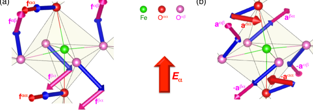
Figure 1: Response of Dzyaloshinskii-Moriya (DM) interactions to electric field in $R3c$ BiFeO₃. Blue arrows denote DM vectors without ${\bf E}$ and red arrows denote the change of DM with ${\bf E}$. (a) FE-induced DM ($\textbf{\emph{D}}_{\rm FE}$) and its derivative vectors (${\bf f}$) with respect to ${\bf E}$. (b) AFD-induced DM ($\textbf{\emph{D}}_{\rm AFD}$) and its derivative vectors (${\bf a}$) with respect to ${\bf E}$. The sign of the vectors alternate due to the AFD nature. Thick- and light-red arrows denote responses of DM to ${\bf E}$ along the $\alpha$ direction when spin bonds are parallel (${\bf f}^{\alpha\alpha}$, ${\bf a}^{\alpha\alpha}$) and perpendicular (${\bf f}^{\alpha\beta}$, ${\bf a}^{\alpha\beta}$) to ${\bf E}$ respectively. The size of the arrows is proportional to the magnitudes of the response to ${\bf E}$. O^αα (O^αβ) denotes oxygens along bonds parallel (perpendicular) to ${\bf E}$, respectively. Bi is not drawn for clarity.

In the lab reference frame $\{x,y,z\}$, regrouping terms for domain 2 with ${\bf x}^{\prime}=[1,0,-1]$ yields $P^{{\rm SC}}_{{\rm FE},\alpha}=\sum_{\beta}\Lambda^{\rm FE}_{\alpha\beta}T_{\beta}$ with

$$\underline{\Lambda}^{\rm FE}=\left\{\begin{array}[]{l}{\bf f}^{xx}\\ {\bf f}^{xy}\\ {\bf f}^{xz}\end{array}\right\}-\left\{\begin{array}[]{l}{\bf f}^{zx}\\ {\bf f}^{zy}\\ {\bf f}^{zz}\end{array}\right\}=\left(\begin{array}[]{ccc}-h&f-g&-f\\ g&2h&g\\ -f&f-g&-h\\ \end{array}\right),$$ (11)

where

$${\bf T}_{1}=\frac{1}{N}\sum_{\langle i,j\rangle^{\bf x}}({\bf S}_{i}\times{\bf S}_{j})$$ (12)

and $f={\bf f}_{\beta}^{\alpha\alpha}$, $g={\bf f}_{\beta}^{\alpha\beta}$, $h={\bf f}_{\gamma}^{\alpha\beta}$.

The second SCP arising from AFD rotations alternates in sign due to the alternating AFD rotations along [111]:

$$P^{\rm SC}_{{\rm AFD},\gamma}=-\frac{\partial{\cal H_{\rm AFD}^{\rm SC}}}{\partial E_{\gamma}}=-\displaystyle\sum_{k,\langle i,j\rangle^{\bf k}}\!\!\frac{(-1)^{n_{i}}}{N}\frac{\partial{\textbf{\emph{D}}^{k}_{{\rm AFD}}}}{\partial E_{\gamma}}\cdot\!\bigl{(}{\bf S}_{i}\times{\bf S}_{j}\!\bigr{)}.$$ (13)

The SCP components ${\bf a}^{k\gamma}=\partial\textbf{\emph{D}}_{\rm AFD}^{k}/\partial E_{\gamma}$ are evaluated in Tab. 1. While the derivative (${\bf a}^{\alpha\alpha}$) of $\textbf{\emph{D}}_{\rm AFD}^{k}$ between spins ${\bf S}_{i}$ and ${\bf S}_{j}$ with ${\bf R}_{j}-{\bf R}_{i}$ parallel to the electric field is nearly anti-parallel to $\textbf{\emph{D}}_{\rm AFD}^{k}$, that (${\bf a}^{\alpha\beta}$) of $\textbf{\emph{D}}_{\rm AFD}^{k}$ between spins with ${\bf R}_{j}-{\bf R}_{i}$ perpendicular to the electric field is perpendicular to $\textbf{\emph{D}}_{\rm AFD}^{k}$, as shown in Fig. 1.

For the spin-cycloid in BiFeO₃, the SCP is simplified as (Appendix D),

$${\bf P}^{\rm SC}_{\rm AFD} = \frac{1}{\sqrt{3}N}\Biggl{\{}\sum_{\langle i,j\rangle^{\bf x}}(-1)^{n_{i}}\underline{\Lambda}^{\rm AFD}\cdot({\bf S}_{i}\times{\bf S}_{i+x})+\sum_{\langle i,j\rangle^{\bf y}}(-1)^{n_{i}}\underline{\Lambda}^{\rm AFD}\cdot({\bf S}_{i}\times{\bf S}_{i+y})$$ (14)

$$+\sum_{\langle i,j\rangle^{\bf z}}(-1)^{n_{i}}\underline{\Lambda}^{\rm AFD}\cdot({\bf S}_{i}\times{\bf S}_{i+z})\Biggr{\}}$$

so that

$$\underline{\Lambda}^{\rm AFD}={\bf a}^{xx}+{\bf a}^{yy}+{\bf a}^{zz}=\left(\begin{array}[]{ccc}s&t&t\\ t&s&t\\ t&t&s\\ \end{array}\right),$$ (15)

where $s=a^{\alpha\alpha}_{\alpha}+2a^{\alpha\beta}_{\beta}$ and $t=a^{\alpha\alpha}_{\beta}+a_{\alpha}^{\alpha\beta}+a_{\gamma}^{\alpha\beta}$ as shown in Tab. 1.

4. Two exchange-striction polarizations

The absence of an inversion center between neighboring spin sites also allows the emergence of exchange-striction (ES) polarizations. Since the scalar product ${\bf S}_{i}\cdot{\bf S}_{j}$ is modified by external perturbations such as temperature, electric or magnetic field, the change in the dot product can induces the ES polarizations. FE and AFD distortions each generates its own ES polarization.

For symmetric exchange couplings, ES is dominated by the response of the nearest-neighbor interaction $J_{1}$:

$${\cal H_{\rm ex}}=-\sum_{\langle i,j\rangle}J_{1}\;{\bf S}_{i}\cdot{\bf S}_{j}=-\sum_{k,\langle i,j\rangle^{\bf k}}J_{1}^{k}\;{\bf S}_{i}\cdot{\bf S}_{j}.$$ (16)

The two ES polarizations ($P^{{\rm ES}}_{{\rm FE}}$, $P^{{\rm ES}}_{{\rm AFD}}$) associated with ${\bf W}_{1}$ and ${\bf W}_{2}$ are closely related to one another. The electric-field derivatives $\underline{\Gamma}$ are given in the cubic coordinate system by

$$P^{{\rm ES}}_{{\rm FE},\alpha}=-\frac{1}{N}\sum_{\alpha}\frac{\partial{\cal H_{\rm ex}}}{\partial{E_{\alpha}}}=\sum_{\beta}\Gamma^{\rm FE}_{\alpha\beta}\,W_{1\beta}$$ (17)

$$\underline{\Gamma}^{\rm FE}=\left(\begin{array}[]{ccc}C_{\parallel}&C_{\perp}&C_{\perp}\\ C_{\perp}&C_{\parallel}&C_{\perp}\\ C_{\perp}&C_{\perp}&C_{\parallel}\\ \end{array}\right),$$ (18)

$$W_{1u}=\frac{1}{N}\sum_{\langle i,j\rangle^{\bf u}}\!{\bf S}_{i}\cdot{\bf S}_{j},$$ (19)

where $C_{\perp}=\partial{J_{1}^{\beta}}/\partial E_{\alpha}$ ($\beta\neq\alpha$) and $C_{\parallel}=\partial J_{1}^{\alpha}/\partial E_{\alpha}$ for spin bonds perpendicular and parallel to the electric field, respectively.

The AFD octahedral rotation is perpendicular to ${\bf z}^{\prime}$. Therefore, the ES polarization associated with AFD is also perpendicular to ${\bf z}^{\prime}$ with

$${\textbf{\emph{P}}^{\rm ES}_{\rm AFD}}=C_{\rm AFD}\,{\bf z}^{\prime}\times{\bf W}_{2},$$ (20)

$$P^{{\rm ES}}_{\rm AFD,\alpha}=\sum_{\beta}\Gamma^{\rm AFD}_{\alpha\beta}\,W_{2\beta}$$ (21)

$$W_{2u}=\frac{1}{N}\sum_{\langle i,j\rangle^{\bf u}}(-1)^{n_{i}}\,{\bf S}_{i}\cdot{\bf S}_{j},$$ (22)

$$\underline{\Gamma}^{\rm AFD}=\left(\begin{array}[]{ccc}0&-(C_{\parallel}\!-\!C_{\perp})&C_{\parallel}\!-\!C_{\perp}\\ C_{\parallel}\!-\!C_{\perp}&0&-(C_{\parallel}\!-\!C_{\perp})\\ -(C_{\parallel}\!-\!C_{\perp})&C_{\parallel}\!-\!C_{\perp}&0\\ \end{array}\right).$$ (23)

Unlike $W_{1u}$, $W_{2u}$ alternates in sign due to opposite AFD rotations between adjacent hexagonal layers.

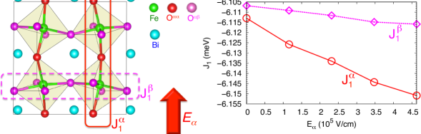
Figure 2: Strong anisotropic response of magnetic exchange ($J_{1}$) to an electric field. The slopes of thick and dotted lines represent derivatives of $J_{1}$ with respect to electric fields parallel ($C_{\parallel}=\partial{J_{1}^{\alpha}}/\partial{E_{\alpha}}$) and perpendicular ($C_{\perp}=\partial{J_{1}^{\beta}}/\partial{E_{\alpha}}$, $\alpha\neq\beta$) to the spin-bond direction calculated from DFT.

The first ES polarization parallel to ${\bf z}^{\prime}$ with coefficient $C_{\rm FE}=(2C_{\perp}+C_{\parallel})$ modulates the FE polarization that already breaks IS above $T_{\rm N}$. The second ES polarization perpendicular to ${\bf z}^{\prime}$ is described by the coefficient $C_{\rm AFD}=C_{\perp}-C_{\parallel}$. The AFD distortion affects the bonds between nearest-neighbor spins in the plane normal to ${\bf z}^{\prime}$ because each oxygen moves along $[0,-1,1]$, $[1,0,-1]$, and $[-1,1,0]$, perpendicular to ${\bf z}^{\prime}$. Thus, the second ES polarization is associated with atomic displacements perpendicular to ${\bf z}^{\prime}$ and parallel to the AFD rotation.

Figure 2 shows a strong anisotropy in the response of magnetic exchange to an electric field. $C_{\perp}$ arises from the change in Fe-O-Fe bond angle due to a polar distortion; $C_{\parallel}$ arises from bond contraction. As shown in the figure, $C_{\parallel}$ is much more sensitive to an electric field than $C_{\perp}$. Since the ME anisotropy $C_{\rm AFD}=C_{\parallel}-C_{\perp}$ produces an ES polarization associated with AFD, the AFD rotation angle is affected by the spin ordering. In particular, the negative sign ($C_{\rm AFD}=-250$ nC/cm²) indicates an increase of the rotation angle with respect to an increase in the dot product ${\bf S}_{i}\cdot{\bf S}_{j}$ because oxygen atoms moving in the AFD plane have a negative effective charge $Z^{*}_{\rm O}({\rm DFT})=-3.3e$.

The anisotropic ES polarization components $C_{\perp}$ and $C_{\parallel}$ cooperatively induce the ES polarization along ${\bf z}^{\prime}$ under the IS broken by the FE polarization. We now obtain a negative $C_{\rm FE}=-350$ nC/cm² with respect to a dynamic electric field in contrast to our previous study lee15 on the response to a static electric field ($C_{\rm FE}=215$ nC/cm²). Appendix B shows the different eigenvectors of the dynamic and force-constant matrices. Fe moves upward with respect to oxygens in the static regime while Fe moves downward in the dynamic regime because its mass is much larger than that of oxygen. Therefore, a static ${\bf E}$ increases the bond angle of Fe-O-Fe (positive $C_{\rm FE}$) but a dynamic ${\bf E}$ decreases the bond angle (negative $C_{\rm FE}$) due to the Goodenough-Kanamori rules goodenough

5. Origin of directional dichroism

The most stringent test yet for the microscopic model proposed above is its ability to predict the NDD, i.e. the weak asymmetry $\Delta\alpha(\omega)$ in the absorption $\alpha(\omega)$ of light when the direction of light propagation is reversed. The absorption of THz light is given by $\alpha(\omega)=(2\omega/c)\,{\rm{Im}}N(\omega)$ where miyahara11 ; miyahara14

$$N(\omega)\approx\sqrt{(\underline{\epsilon}_{ii}+\chi^{ee}_{ii}(\omega))(1+\chi^{mm}_{jj}(\omega))}\pm\chi^{me}_{ji}(\omega)$$ (24)

is the complex refractive index for a linearly polarized beam, $\underline{\chi}^{ee}$, $\underline{\chi}^{mm}$ and $\underline{\chi}^{me}$ are the dielectric, magnetic, and magnetoelectric susceptibility tensors describing the dynamical response of the spin system kezsmarki11 ; bordacs12 ; miyahara11 ; szaller13 and $\underline{\epsilon}$ is the dielectric constant. Subscripts $i$ and $j$ refer to the electric and magnetic polarization directions, respectively. The second term, which depends on the light propagation direction and produces NDD, is separated from the mean absorption by writing $N(\omega)=\bar{N}(\omega)\pm\chi^{me}_{ji}(\omega)$.

Summing over the spin-wave modes $n$ at the cycloidal ordering wavevector ${\bf Q}$, $\Delta\alpha(\omega)=(4\omega/c)\,{\rm{Im}}\chi^{me}(\omega)$ is given by

$$\Delta\alpha(\omega)=\sum_{n}A_{n}\,\delta(\omega-\omega_{n}),$$ (25)

$$A_{n}=NX\omega_{n}\,\rm{Re}\Bigl{\{}\rho_{n0}\mu_{0n}\Bigr{\}},$$ (26)

$$\rho_{0n}=\langle 0|P^{\rm SD}\cdot{\bf e}/{\cal V}|{\it n}\rangle,\;\;\;\;\;\;\;\;\;\;\;\;\mu_{0n}=\langle 0|{\bf M}\cdot{\bf h}/\mu_{\rm B}|{\it n}\rangle,$$ (27)

where ${\bf M}=(2\mu_{\rm B}/N)\sum_{i}{\bf S}_{i}$ is the magnetization, ${\cal V}=a^{3}$ is the volume per Fe site, ${\bf P}^{\rm SD}/{\cal V}=({\textbf{P}}^{\rm ES}+{\textbf{P}}^{\rm SC})/{\cal V}$ is the net spin-driven polarization given in units of nC/cm², and

$$X=\frac{4\pi\mu_{\rm B}}{\hbar}\frac{{\rm nC}}{{\rm cm}^{2}}=\frac{0.1388}{{\rm cm}}.$$ (28)

The THz electric and magnetic fields are polarized in the electric (${\bf e}$) and magnetic (${\bf h}$) directions, respectively.

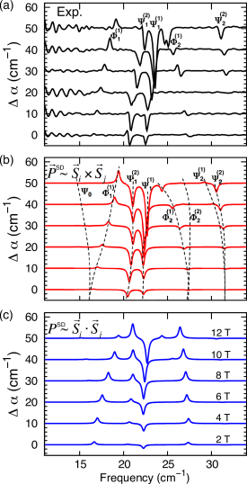
Figure 3: Origin of the strong directional dichroism in BiFeO₃. (a) The experimental NDD ($\Delta$ $\alpha$) with static magnetic field from 2 to 12 T and oscillating electric field along $[1,-1,0]$. The predicted NDD using spin-current (b) and exchange-striction (c) polarizations. $i,j$ denotes nearest neighbors.

Table 1: SD-polarizations from exchange striction, spin current and single-ion anisotropy. Shown are the calculated (LSDA+$U$) electric-field derivatives of $J_{1}$, $\textbf{\emph{D}}_{\rm FE},\textbf{\emph{D}}_{\rm AFD}$, and $K$. The upper left and right scripts denote the directions of the spin bond and electric field, respectively. $f^{\alpha\alpha}_{\beta}=-f^{\alpha\alpha}_{\gamma}$, $f^{\alpha\beta}_{\gamma}=-f^{\beta\alpha}_{\gamma}$, and $a^{\alpha\alpha}_{\beta}=a^{\alpha\alpha}_{\gamma}$ by $R3c$ symmetry as in Appendix C. $\alpha$, $\beta$, and $\gamma$ are in ascending order so that $\epsilon_{\alpha\beta\gamma}=1$.

	SCP from $\textbf{\emph{D}}_{\rm FE}$			SCP from $\textbf{\emph{D}}_{\rm AFD}$		ES polarization from $J_{1}$
	$f^{\alpha\alpha}_{\beta}$	$f^{\alpha\beta}_{\gamma}$	$f^{\alpha\beta}_{\beta}$	$a^{\alpha\alpha}_{\alpha}$+2$a^{\alpha\beta}_{\beta}$	$a_{\beta}^{\alpha\alpha}+a_{\alpha}^{\alpha\beta}+a_{\gamma}^{\alpha\beta}$	$C_{\rm AFD}$	$C_{\rm FE}$
LSDA+$U$	9	17	14	17	$-19$	$-250$	$-350$
Directional dichroism	36	29	29	28	$-7.2$	-	-

For each field orientation and set of propagation vectors ${\bf e}$ and ${\bf h}$, the integrated weight of every spectroscopic peak at $\omega_{n}$ is compared with the measured values, thereby eliminating estimates of the individual peak widths. Experimental results for the NDD with field along ${\bf m}=[1,-1,0]$ are plotted in Fig. 3(a) for ${\bf e}=[1,-1,0]$. Fits to the NDD are based on the plotted 2, 4, 6, 8, 10, and 12 T data sets. For each data set (${\bf h}$ polarizations per field), we evaluate the integrated weights for the 8 modes nagel13 $\Psi_{0}$, $\Phi_{1}^{(1)}$, $\Psi_{1}^{(1,2)}$, $\Phi_{2}^{(1,2)}$, and $\Psi_{2}^{(1,2)}$ between roughly 12 and 35 cm^-1.

From the comparison of Figs. 3(a) and (b), the NDD for ${\bf m}=[1,-1,0]$ is dominated by the two sets of SC polarizations ${\bf P}^{{\rm SC}}_{\rm FE}$ and ${\bf P}^{{\rm SC}}_{\rm AFD}$ associated with the DM interactions $\textbf{\emph{D}}_{\rm FE}$ and $\textbf{\emph{D}}_{\rm AFD}$, respectively. Tab. 1 indicates that the fitting results are not significantly changed by including the ES polarizations. As shown in Figs. 3(c) and (d), which minimizes $\chi^{2}$ with respect to the experimental measurements Istvan , ES polarizations by themselves cannot produce the observed NDD.

Comparing our results to the fits to the NDD, the various components of the spin-current polarizations in BiFeO₃ are captured by first-principles calculations in Tab. 1. The optical ME effect responsible the NDD is dominated by the spin-current polarizations and is not strongly affected by the exchange-striction terms. This selective feature originates from the nature of the spin dynamics in BiFeO₃. Due to the very small single-ion anisotropy on the S = 5/2 Fe³⁺ spins, each magnon mode can be described as the pure precession of the Fe³⁺ spins: the oscillating component $\delta{\bf S}_{i}^{\omega}$ of the spin on site $i$ is perpendicular to its equilibrium direction ${\bf S}_{i}^{0}$. Since neighboring spins are close to collinear in the long-range spin cycloid of BiFeO₃, a dynamic polarization is effectively induced by spin-current terms such as ${\bf S}_{i}^{0}\times\delta{\bf S}_{i+1}^{\omega}$. However, the dynamic polarization generated by exchange-striction terms ${\bf S}_{i}^{0}\cdot\delta{\bf S}_{i+1}^{\omega}$ is almost zero. The spin stretching modes observed in strongly anisotropic magnets miyahara11 ; penc12 does not appear in BiFeO₃.

Nevertheless, our DFT calculations underestimate the NDD fitting results in Tab. 1. We can think of five reasons for this underestimation. First, a larger dielectric constant ($\epsilon$) could produce better agreement between DFT and NDD since the spin-driven polarizations are proportional to the dielectric constant that enters Eq. 9. Second, consideration of an electrically-induced polarization ($P^{\rm ind}_{\beta}$, $\beta\neq\alpha$) not parallel to electric field ($P^{\rm ind}_{\alpha}$) could improve the results quantitatively. Third, higher-frequency polar modes which were not considered here also can affect NDD. Fourth, a smaller Hubbard $U$ will increase the spin-driven polarizations and improve the agreement with the experimental fits. Fifth, magnon modes were observed between $\nu=15$ and 40 cm^-1 while we calculated the ME couplings in the dynamical limit. The crossover frequency $\omega_{c}$ between static and dynamical behavior lies between 0 and the polar phonon at $\omega=78$ cm^-1. If $\omega_{c}$ lies in the middle of the measured frequencies, then the polarization parameters may differ from the dynamical couplings evaluated here.

6. Discussion

Anchoring first-principles calculations to the right microscopic Hamiltonian is crucial to understand the ME couplings in complex multiferroic systems. With two sets of spin-current polarizations derived from the two distinct structural distortions, BiFeO₃ is a good example of how our atomistic approach works for complex materials beyond the simple inverse DM interaction iDM with only one spin-current polarization.

The advantages (large FE polarization, high $T_{\rm C}$, and $T_{\rm N}$) of BiFeO₃ have also turned out to be major obstacles to understanding the ME couplings that produce the spin-driven polarizations below $T_{\rm N}$. Leakage currents and the preexisting large FE polarization at high temperatures have hampered magneto-capacitance measurements and hidden the spin-driven polarizations. Although recent neutron-scattering measurements lee13 imply a large ES polarization, most other ME polarizations are unknown. However, NDD measurements combined with first-principles calculations based on a microscopic model reveal the hidden SC-induced polarizations. In particular, this approach allows us to disentangle the delicate spin-current polarizations and the hidden ES polarizations associated with AFD rotation that cannot be captured in any other way. We envision that intrinsic methods such as NDD will reveal hidden ME couplings in many materials and rekindle the investigation of type-$I$ multiferroics.

Acknowledgements

We acknowledge discussions with H. Kim, E. Bousquet, Nobuo Furukawa, S. Miyahara, J. Musfeldt, U. Nagel, S. Okamoto, S. Bordács and T. Rõõm. Research sponsored by the U.S. Department of Energy, Office of Basic Energy Sciences, Materials Sciences and Engineering Division. I.K. was supported by the Hungarian Research Fund OTKA K 108918. We also thank Hee Taek Yi and Sang-Wook Cheong for preparation of the BiFeO₃ sample.

Appendix A Simplified form of Dzyaloshinskii-Moriya (DM) interactions.

A.1 FE-induced Dzyaloshinskii-Moriya (DM) interaction.

Since the FE vectors $\textbf{\emph{D}}_{\rm FE}^{k}$ are given by (0, $D_{\rm FE}$, $-D_{\rm FE}$), ($-D_{\rm FE}$, $D_{\rm FE}$, 0), and ($D_{\rm FE}$, $-D_{\rm FE}$, 0) between nearest spins along ${\bf x}$, ${\bf y}$, and ${\bf z}$, respectively, the FE-induced DM interaction can be transformed as:

$${\cal H}_{\rm FE}^{\rm SC}=\sum_{{\bf R}_{i},{\bf R}_{j}={\bf R}_{i}+{\bf e}_{k}}\textbf{\emph{D}}_{\rm FE}^{k}\cdot({\bf S}_{i}\times{\bf S}_{j})=D_{1}\,\sum_{{\bf R}_{i},{\bf R}_{j}={\bf R}_{i}+{\bf e}_{k}}({\bf z}^{\prime}\times{\bf e}_{k}/a)\cdot({\bf S}_{i}\times{\bf S}_{j}),$$ (29)

where $D_{1}=D_{\rm FE}\approx 154$ nC/cm² is now larger by $\sqrt{2}$ than in previous work fishman13a .

A.2 AFD-induced Dzyaloshinskii-Moriya (DM) interaction.

The AFD interactions $\textbf{\emph{D}}_{\rm AFD}^{k}$ along ${\bf x}$, ${\bf y}$, and ${\bf z}$ can be written

$${\textbf{\emph{D}}_{{\rm AFD}}^{x}}=B({\bf y}+{\bf z})+A{\bf x},$$ (30)

$${\textbf{\emph{D}}_{{\rm AFD}}^{y}}=B({\bf z}+{\bf x})+A{\bf y},$$ (31)

$${\textbf{\emph{D}}_{{\rm AFD}}^{z}}=B({\bf x}+{\bf y})+A{\bf z}.$$ (32)

For the magnetic domain with wavevector along $[1,0,-1]$,

$${\cal H}_{\rm AFD}^{\rm SC} = \sum_{{\bf R}_{i},{\bf R}_{j}={\bf R}_{i}+{\bf e}_{k}}\,(-1)^{n_{i}}\textbf{\emph{D}}_{\rm AFD}^{k}\cdot({\bf S}_{i}\times{\bf S}_{j})$$ (34)

$$= \sqrt{3}\sum^{\prime}_{{\bf R}_{i}}{\bf z}^{\prime}\cdot\Bigl{\{}B\;{\bf S}_{r}\times({\bf S}_{{\bf R}_{i}+a{\bf x}}+2{\bf S}_{{\bf R}_{i}+a{\bf y}}+{\bf S}_{{\bf R}_{i}+a{\bf z}})+A\;{\bf S}_{{\bf R}_{i}}\times({\bf S}_{{\bf R}_{i}+a{\bf x}}+{\bf S}_{{\bf R}_{i}+a{\bf z}})\Bigr{\}}$$

$$+ \sum^{\prime}_{{\bf R}_{i}}{\bf y}^{\prime}\cdot\Bigl{\{}(B-A)\;{\bf S}_{{\bf R}_{i}}\times({\bf S}_{{\bf R}_{i}+a{\bf x}}-2{\bf S}_{{\bf R}_{i}+a{\bf y}}+{\bf S}_{{\bf R}_{i}+a{\bf z}})\Bigr{\}}$$

$$\approx \sqrt{3}\sum^{\prime}_{{\bf R}_{i}}{\bf z}^{\prime}\cdot\Bigl{\{}B\;{\bf S}_{{\bf R}_{i}}\times({\bf S}_{{\bf R}_{i}+a{\bf x}}+2{\bf S}_{{\bf R}_{i}+a{\bf y}}+{\bf S}_{{\bf R}_{i}+a{\bf z}})+A\;{\bf S}_{{\bf R}_{i}}\times({\bf S}_{{\bf R}_{i}+a{\bf x}}+{\bf S}_{{\bf R}_{i}+a{\bf z}})\Bigr{\}},$$

$$\approx \sqrt{3}(4B+2A)\sum^{\prime}_{{\bf R}_{i}}{\bf z}^{\prime}\cdot({\bf S}_{{\bf R}_{i}}\times{\bf S}_{{\bf R}_{i}+a{\bf y}})$$

where the primed sum over ${\bf R}_{i}$ is restricted to either $n_{i}$ odd or even hexagonal layers. Because ${\bf S}_{{\bf R}_{i}+a{\bf x}}-2{\bf S}_{{\bf R}_{i}+a{\bf y}}+{\bf S}_{{\bf R}_{i}+a{\bf z}}$ is of order $\delta^{2}\sim 2\times 10^{-5}$, the ${\bf z}^{\prime}$ term dominates.

Previously, the second DM term was written

$${\cal H}_{\rm AFD}^{\rm SC} = D_{2}\sum_{{\bf R}_{i},{\bf R}_{j}={\bf R}_{i}+{\bf e}_{k}}\,(-1)^{n_{i}}{\bf z}^{\prime}\cdot({\bf S}_{i}\times{\bf S}_{j})$$ (35)

$$= 2\sqrt{3}D_{2}\sum^{\prime}_{{\bf R}_{i}}{\bf z}^{\prime}\cdot({\bf S}_{{\bf R}_{i}}\times{\bf S}_{{\bf R}_{i}+a{\bf x}}+{\bf S}_{{\bf R}_{i}}\times{\bf S}_{{\bf R}_{i}+a{\bf y}}+{\bf S}_{{\bf R}_{i}}\times{\bf S}_{{\bf R}_{i}+a{\bf z}})$$

$$\approx 6\sqrt{3}D_{2}\sum^{\prime}_{{\bf R}_{i}}{\bf z}^{\prime}\cdot({\bf S}_{{\bf R}_{i}}\times{\bf S}_{{\bf R}_{i}+a{\bf y}})$$

Therefore, $D_{2}=(A+2B)/3=0.064$ meV, which is in excellent agreement with previous determinations of $D_{2}$ [fishman13a, ].

Appendix B Eigenvectors of dynamic and force-constant matrix responsible for the different C_FE.

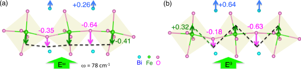
Figure 4: Distinct atomic responses to dynamic and static electric fields. The lowest-frequency eigenvectors of dynamic matrix (a) and of force-constant matrix (b) are compared. Note that the polar displacement in the dynamic limit ($\omega$ = 78 cm^-1) increases the Fe-O-Fe bond angle (dotted line) while the displacement decreases in the static limit.

We note in the paper that C_FE is negative from the eigenmode of the dynamic matrix while it is positive from eigenmode of force-constant matrix lee15 . This difference originates from the opposite change of the Fe-O-Fe bond angle. The bond angle increases in the static limit (a) while it decreases in the dynamic limit (b) ($\omega$ = 78 cm^-1). The different responses to electric field give rise to opposite sign of C_FE.

Appendix C Spin-current polarization components in cubic axis

Defining ${\bf f}^{k\gamma}=\partial\textbf{\emph{D}}_{\rm FE}^{k}/\partial E_{\gamma}$ (f denotes FE distortion),

$${\textbf{\emph{D}}_{{\rm FE}}^{x}}=(0,D,-D),\;\;\;\;\;\;{\textbf{\emph{D}}_{{\rm FE}}^{y}}=(-D,0,D),\;\;\;\;\;\;{\textbf{\emph{D}}_{{\rm FE}}^{z}}=(D,-D,0)$$ (36)

$$\vspace{4mm}{\bf f}^{xx}=(0,f,-f),\;\;\;\;\;\;{\bf f}^{yx}=(-g,0,-h),\;\;\;\;\;\;{\bf f}^{zx}=(g,h,0),$$ (37)

$${\bf f}^{xy}=(0,g,h),\;\;\;\;\;\;{\bf f}^{yy}=(-f,0,f),\;\;\;\;\;\;{\bf f}^{zy}=(-h,-g,0),$$ (38)

$${\bf f}^{xz}=(0,-h,-g),\;\;\;\;\;\;{\bf f}^{yz}=(h,0,g),\;\;\;\;\;\;{\bf f}^{zz}=(f,-f,0),$$ (39)

where $f\equiv f^{\alpha\alpha}_{\beta},g\equiv f^{\alpha\beta}_{\beta}$, and $h\equiv f^{\alpha\beta}_{\gamma}$.

Defining ${\bf a}^{k\gamma}=\partial\textbf{\emph{D}}_{\rm AFD}^{k}/\partial E_{\gamma}$ (a denotes AFD distortion),

$${\textbf{\emph{D}}_{{\rm AFD}}^{x}}=(A,B,B),\;\;\;\;\;\;{\textbf{\emph{D}}_{{\rm AFD}}^{y}}=(B,A,B),\;\;\;\;\;\;{\textbf{\emph{D}}_{{\rm AFD}}^{z}}=(B,B,A),$$ (40)

$$\hskip 45.5244pt{\bf a}^{xx}=(a,b,b),\;\;\;\;\;\;{\bf a}^{yx}=(d,c,e),\;\;\;\;\;\;{\bf a}^{zx}=(d,e,c),$$ (41)

$${\bf a}^{xy}=(c,d,e),\;\;\;\;\;\;{\bf a}^{yy}=(b,a,b),\;\;\;\;\;\;{\bf a}^{zy}=(e,d,c),$$ (42)

$${\bf a}^{xz}=(c,e,d),\;\;\;\;\;\;{\bf a}^{yz}=(e,c,d),\;\;\;\;\;\;{\bf a}^{zz}=(b,b,a),$$ (43)

where $a\equiv a_{\alpha}^{\alpha\alpha},b\equiv a_{\beta}^{\alpha\alpha},c\equiv a^{\alpha\beta}_{\alpha},d\equiv a^{\alpha\beta}_{\beta}$, and $e\equiv a^{\alpha\beta}_{\gamma}$.

Appendix D Simplification of spin-current polarization (${\bf a}^{\alpha\beta}$) from antiferrodistortive DM ($\textbf{\emph{D}}_{\rm AFD}$)

For domain 2 with ${\bf x}^{\prime}=[1,0,-1]$,

(44)

$${\cal T}_{x}=\frac{1}{\sqrt{3}}{\cal T}_{z^{\prime}}-\frac{1}{\sqrt{6}}{\cal T}_{y^{\prime}}\;\;\;\;{\cal T}_{y}=\frac{\sqrt{6}}{3}{\cal T}_{y^{\prime}}+\frac{1}{\sqrt{3}}{\cal T}_{z^{\prime}}\;\;\;\;{\cal T}_{z}={\cal T}_{x}\;\;\;\;\;\Big{(}{\cal T}_{k}\equiv\frac{3}{N}\sum_{i}(-1)^{n_{i}}({\bf S}_{i}\times{\bf S}_{i+k})\Big{)}$$ (45)

The spin-driven polarization associated with $\textbf{\emph{D}}_{\rm AFD}$ is

$$P^{\rm SC}_{x} = {\bf a}^{xx}\cdot{\cal T}_{x}+{\bf a}^{yx}\cdot{\cal T}_{y}+{\bf a}^{zx}\cdot{\cal T}_{z},$$ (46)

$$= \frac{1}{\sqrt{6}}(-{\bf a}^{xx}+2{\bf a}^{yx}-{\bf a}^{zx})\cdot{\cal T}_{y^{\prime}}+\frac{1}{\sqrt{3}}({\bf a}^{xx}+{\bf a}^{yy}+{\bf a}^{zz})\cdot{\cal T}_{z^{\prime}}$$ (47)

$$\approx \frac{1}{\sqrt{3}}({\bf a}^{xx}+{\bf a}^{yy}+{\bf a}^{zz})\cdot{\cal T}_{z^{\prime}}$$ (48)

Similarily,

$$P^{\rm SC}_{y} \approx \frac{1}{\sqrt{3}}({\bf a}^{xx}+{\bf a}^{yy}+{\bf a}^{zz})\cdot{\cal T}_{z^{\prime}}$$ (49)

$$P^{\rm SC}_{z} \approx \frac{1}{\sqrt{3}}({\bf a}^{xx}+{\bf a}^{yy}+{\bf a}^{zz})\cdot{\cal T}_{z^{\prime}}$$ (50)

Therefore, in the local frame,

$$P^{\rm SC}_{{\bf x}^{\prime}} = P^{\rm SC}_{{\bf y}^{\prime}}=0,$$ (51)

$$P^{\rm SC}_{{\bf z}^{\prime}} = \frac{1}{\sqrt{3}}(P^{\rm SC}_{x}+P^{\rm SC}_{y}+P^{\rm SC}_{z})=\frac{1}{3}({\bf a}^{xx}+{\bf a}^{yy}+{\bf a}^{zz})\cdot{\cal T}_{z^{\prime}}.$$ (52)

The polarization matrix used to evaluate the NDD is given by

$${\bf a}^{xx}+{\bf a}^{yy}+{\bf a}^{zz}=\left(\begin{array}[]{ccc}a+2d&b+c+e&b+c+e\\ b+c+e&a+2d&b+c+e\\ b+c+e&b+c+e&a+2d\\ \end{array}\right)$$ (53)

where $a+2d=17$ nC/cm² and $b+c+e=-19$ nC/cm² are obtained from first principles as given in Tab.I of the paper. ($a\equiv a_{\alpha}^{\alpha\alpha}=4.1$ nC/cm², $b\equiv a_{\beta}^{\alpha\alpha}=-21$ nC/cm², $c\equiv a^{\alpha\beta}_{\alpha}=-6.7$ nC/cm², $d\equiv a^{\alpha\beta}_{\beta}=6.4$ nC/cm², and $e\equiv a^{\alpha\beta}_{\beta}=8.9$ nC/cm².)

References

(1) Katsura H, Nagaosa N and Balatsky A V
2005 Phys. Rev. Lett.95, 057205;
Mostovoy M
2006 Phys. Rev. Lett.96, 067601;
Sergienko I A and Dagotto E
2006 Phys. Rev. B73, 094434
(2) Teague J R, Gerson R and James W J
1970 Solid State Commun.8, 1073
(3) Sosnowska I, Peterlin-Neumaier T and Steichele E
1982 J. Phys. C: Solid State Phys.15, 4835
(4) Lebeugle D, Colson D, Forget A and Viret M,
2007 Appl. Phys. Lett.91, 022907
(5) Kadomtseva A M, Zvezdin, A.K., Popv Y F, Pyatakov A P and Vorob’ev G P
2004 JTEP Lett.79, 571
(6) Tokunaga M, Azuma M and Shimakawa Y
2010 J. Phys. Soc. Jpn.79, 064713
(7) Zvezdin A K and Pyatakov A P
2012 Europhys. Lett.99, 57003
(8) Park J et al.
2011 J. Phys. Soc. Jpn.80, 114714
(9) Lebeugle D, Colson D, Forget A, Viret M, Bataille A M and Gukasov A
2008 Phys. Rev. Lett.100, 227602
(10) Ramazanoglu M, Ratcliff II W, Choi Y J, Lee S, Cheong S-W and Kiryukhin V
2011 Phye. Rev. B83, 174434
(11) Sosnowska I and Przenioslo R
2011 Phys. Rev. B84, 144404
(12) Lee S et al.
2013 Phys. Rev. B88, 060103(R)
(13) Rovillain P et al.
2010 Nat. Mater.9, 975
(14) Fiebig M 2005 J. Phys. D38, R123R152
(15) Kézsmárki I, Kida N, Murakawa H, Bordàcs S, Onose Y and Tokura Y
2011 Phys. Rev. Lett.106, 057403
(16) Takahashi Y, Shimano R, Kaneko Y, Murakawa H and Tokura Y
2012 Nat. Phys.8, 121
(17) Bordàcs S et al.
2012 Nat. Phys.8, 734
Arima, T 2008 J. Phys. Condens. Matter20, 434211
(18) Miyahara S and Furukawa N
2012 J. Phys. Soc. Japan81, 023712
(19) Szaller D, Bordàcs S and Kézsmáki I 2013
Phys. Rev. B87, 014421;
Kézsmáki I et al. 2014 Nat. Commun.5, 3203
(20) Chen H B and Li Y-Q
2013 App. Phy. Lett.102, 252906
(21) Pyatakov A P and Zvezdin A K
2009 Eur. Phys. J. B71, 419
(22) Fishman R S
2013 Phys. Rev. B87, 224419
(23) Fishman R S, Haraldsen J T, Furukawa N and Miyahara S
2013 Phys. Rev. B87, 134416
(24) Weingart C, Spaldin N, and Bousquet E
2012 Phys. Rev. B86, 094413
(25) Ederer C and Spaldin N A
2005 Phys. Rev. B71, 060401(R)
(26) Blöchl P E
1994 Phys. Rev. B50, 17953
(27) Kresse G and Joubert D
1999 Phys. Rev. B59, 1758
(28) Lobo R P et al.
2007 Phys. Rev. B76, 172105
(29) Lee J H and Fishman R S
arXiv:1506.04595.
(30) Goodenough J B 1993 Magnetism and the chemical bond (John Wiley and Sons, New York-London)
(31) Miyahara S and Furukawa N 2011 P J. Phys. Soc. Japan80, 073708
(32) Miyahara S. and Furukawa N 2014 Phys. Rev. B89, 195145
(33) Nagel U et al.
2013 Phys. Rev. Lett.110, 257201
(34) Kézsmáki I et al. (submitted).
(35) Penc K et al.
2012 Phys. Rev. Lett.108, 257203