Wireless Coverage Area Computation and Optimization

Abstract

A wireless network’s design must include the optimization of the area of coverage of its wireless transmitters - mobile and base stations in cellular networks, wireless access points in WLANs, or nodes on a transmit schedule in a wireless ad-hoc network. Typically, the coverage optimization for the common channels is “solved” by spatial multiplexing, i.e. keeping the access networks far apart. However, with increasing densities of wireless network deployments (including the Internet-of-Things) and paucity of spectrum, and new developments like whitespace devices and self-organizing, cognitive networks, there is a need to manage interference and optimize coverage by efficient algorithms that correctly set the transmit powers to ensure that transmissions only use the power necessary.

In this work we study methods for computing and optimizing interference-limited coverage maps of a set of transmitters. We progress successively through increasingly realistic network scenarios. We begin with a disk model with a fixed set of transmitters and present an optimal algorithm for computing the coverage map. We then enhance the model to include updates to the network, in the form of addition or deletion of one transmitter. In this dynamic setting, we present an optimal algorithm to maintain updates to the coverage map. We then move to a more realistic interference model - the SINR model. For the SINR model we first show geometric bases for coverage maps. We then present a method to approximate the measure of the coverage area. Finally, we present an algorithm that uses this measure to optimize the coverage area with minimum total transmit power.

To my family, for giving me selfless support for my selfish endeavor.

Chapter 1 Introduction

A wireless network is a communication network in which network nodes communicate with each other over wireless media. Wireless communication between two nodes involves the transmission of radio signals from one node (the transmitter) which are then decoded by the intended node (the receiver). Successful decoding of a radio signal requires sufficient receive signal energy at the receiver. Radio signals from simultaneous transmissions also typically interfere with each other, and receivers are unable to decode signals that are disrupted by interfering transmissions.

The set of locations at which potential receivers in the network are able to decode transmissions intended for them is the coverage map of the wireless network. For example, Figure 1.1 shows a typical wireless network with a fixed set of transmitters. The shaded area in this figure shows the network’s coverage map.

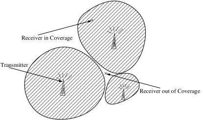
Figure 1.1: Example of Coverage Map with 3 Transmitters

1.1 Motivation and goals

A key service quality indicator of a wireless network is the size or measure of its coverage map, i.e. the coverage area. The maintenance of an adequately large coverage area is achieved by coverage area maximization. The objective function for this optimization is the coverage area, and the optimization variables and constraints are drawn from the network topology and energy profile, such as the transmitter and receiver location constraints, channels available for transmission, receive sensitivity and environmental noise, transmission schedules, MAC parameters (for example, the backoff algorithm and retransmit policy), and available and allowed transmit power for individual transmitters and the network.

Both speed and accuracy of coverage area measurement and maximization are necessary to manage the phenomenal expanse of applications on the wireless medium - cell sites, mobile subscribers, access points, WiFi-connected portable devices, and on-demand mobile software.

Infrastructure wireless networks, like WLANs and cellular networks, have their wireless hops anchored to access points and base stations. In these networks, much of the network coverage optimization is done before the infrastructure is deployed. In ad-hoc networks, in contrast, coverage optimization happens while the network is in operation. In both cases coverage is limited by the RF environment - due to path loss, fading and shadowing - and by interference from simultaneous transmissions on conflicting bands. In cellular networks, the optimization begins as early as designing the regulatory framework - apportioning RF bands by country, region and network operator - to limit interference and thereby, improve coverage. WLANs use non-regulated bands, and hence the interference management for coverage optimization happens at network deployment. Some of the coverage optimization happens during the signalling between device and access point (or base station): the device is informed of specific channels in the band to use for each transmission in order to avoid interference.

Transmitter locations may be restricted due to availability of shelter, power source, cooling, or other infrastructure restrictions. The schedule of transmissions too may not be within the control of the designer, given the large variety of applications. Once a network deployment location is chosen the only variables available for coverage optimization possibly are the channels, number of transmitters and their transmit powers.

Furthermore, optimization methods that allow the designer to experiment with configurations quickly are desirable. Such optimization methods are also required for self-management of wireless networks, where the transmitters dynamically vary their parameters to increase coverage.

1.2 Coverage Maps

An intermediate step in designing to optimize coverage is the computation of the ‘coverage map’ for a given set of transmitters. By coverage map we mean the set of feasible locations for placement of receivers such that each receiver can decode correctly a transmission intended for it. Our rationale for suggesting this step is that computing the coverage map may validate an optimum choice of the network’s parameters - for example, the transmitter locations.

Computing and then optimizing the coverage map requires consideration of some basic constraints of wireless transmissions. The constraints we focus on are the following: wireless transmission energy reduces with distance, and simultaneous transmissions in close proximity of the receiver cause interference. Interference at a receiver may be avoided by ensuring that transmissions are only on a single ‘channel’ - fundamentally: frequency, time-slot, or orthogonal code. This may be feasible in infrastructure networks, since link control protocols are available to transmit out-of-band channel information to the receiver. However, in less regulated networks, like wireless ad-hoc networks, simultaneous transmission and reception on the same channel may be unavoidable, and automated self-management is required.

The first step in the computation of the coverage map is the computation of the coverage map for a single ‘channel’. Suppose the coverage map of a given set of transmitters for one channel is known. Then the designer can attempt to optimize coverage by varying the location of the transmitters or their transmission power, or by employing more channels.

While an exact coverage map can be computed for disk models, we shall see that for the SINR model, we can only estimate the area in coverage - since the coverage boundaries are not defined by closed-form equations. Extending coverage estimation beyond the geometric SINR is further complicated by irregular coverage areas, coverage areas that change shape due to fading and shadowing, interference caused by transmitters outside the administrative control of the network, and asymmetric channel conditions between the communicating pair.

1.3 Statement of Work

This thesis contributes new algorithms that: 1) compute the coverage map of a wireless network for different wireless topology models, and 2) find an optimal assignment of transmission parameters that maximizes the coverage area. The algorithms for computing the coverage map report the boundary of the set of points in coverage. For wireless models in which geometric computation of the boundary is inefficient, we show an algorithm that reports a bounded-accuracy estimate of the coverage area. Further, we show an algorithm for optimizing (maximizing) the coverage area of a given network under topology and energy constraints.

We first consider the problem of computing the coverage map for a single channel, modeling the network with the ‘protocol model’ of Gupta et al. [1].

1. Transmissions occur only in the 2-dimensional plane.

2. Each transmitter’s transmission range is a circular disk centered around it, and its interference range is a larger concentric disk.

3. The coverage region of a transmitter is the set of points lying on its transmission disk and outside every other transmitter’s interference disk.

The coverage map is thus the union of the coverage regions of all transmitters.

Figure 1.2 shows an example of a coverage map in the protocol model.

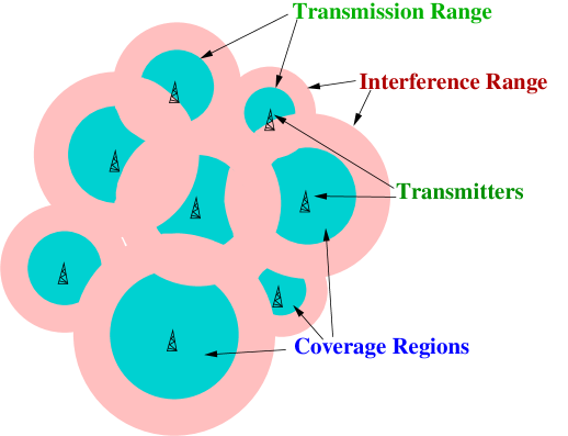
Figure 1.2: A Coverage Map in the Protocol Model

In the protocol model, coverage is decided by set-membership alone - coverage regions being points inside appropriate transmission and interference ranges. This allows us to compute the coverage map efficiently using simple computational geometric primitives. However, this model precludes path loss - the loss of transmission energy with distance from the transmitter.

In Chapter 3 we demonstrate a method for computing the coverage map (for a single channel) under our model. This method requires the entire set of transmitters to be known a priori. However, the designer would have to re-calculate the coverage map for an incremental change in the network, like for example, addition of a new transmitter. In Chapter 4 we extend these results to allow maintenance of the coverage map when one transmitter is added or removed at a time.

In Chapter 5, we explore the coverage problem for a more ‘realistic’ model - the SINR (Signal-to-Interference-plus-Noise-Ratio) model, also called Physical Model by Gupta et al. [1]. We observe that partitioning methods similar to the protocol model studied earlier can be employed - each coverage region corresponds to a partition. However, there are differences in the shapes of the curves enclosing the coverage regions, and hence their representation in coverage computation is different.

In Chapter 6 we propose a simple algorithm that finds an optimal transmit power assignment that maximizes the coverage area of a set of transmitters operating on the same channel. This algorithm uses a coverage estimation function for the coverage area that may be adapted to any deterministic coverage model. We demonstrate the efficiency of this algorithm experimentally using the SINR model to compare it with other algorithms. We also note how the algorithm can be extended to a generic coverage model.

Chapter 2 Literature Review

A recent survey by Phillips et al. [2] covers various coverage mapping methods and transmission models reported over the past few decades. This work considers the problems of computing and optimizing the coverage map for a single channel. It is inspired by the asymptotic capacity limits for wireless networks espoused in the protocol and physical models by Gupta et al. [1].

Our work in coverage map computation generalizes the coverage map computation reported by So et al. [3]. They compute the coverage map for a static wireless sensor network without considering interference. Our ideas for coverage map computation are inspired by generalizations of Voronoi diagrams reported by Aurenhammer et al. in [4], [5], and [6]. The extensions of these ideas to dynamic coverage maps has been influenced by the works on randomized geometric algorithms from Mulmuley ([7]), Aragon et al. [8], and Clarkson et al. [9]. Our work on the coverage map in the SINR model is related to research by Avin et al. [10], who report an approximation algorithm that decides membership of a point in an SINR coverage map.

Our approach to coverage optimization extends that of ‘successive refinement’ by Ahmed et al. [11] that reports optimum transmit power assignments to access points assuming a protocol model. A recent work by Plets et al. [12] describes a tool for optimal design for indoor wireless LANs. Optimal placement of transmitters in bounded geometric areas (modeling typical room shapes) has been recently reported by Yu et al. [13]. Our optimization procedure is inspired by Mudumbai et al. [14]. They report a randomized procedure to synchronize multiple transmissions to send a common message coherently in a distributed beamforming system.

Some optimization problems in link scheduling and power control in the SINR model are closely related to our problem. Goussevskaia et al. [15] show that a discrete problem of ‘single-shot scheduling’ with weighted links is NP-hard. Lotker et al. [16] and Zander et al. [17] give efficient algorithms for optimizing the maximum achievable SINR in a set of links. Yates et al. [18] report an algorithm to optimize the total uplink transmit power for users served by a base station, assuming that all users meet the minimum SINR constraint. A recent study by Altman et al. [19] considers SINR games played co-operatively and co-optively between base stations to maximize coverage area for mobile receivers or determine optimal placement for base stations themselves.

A recent study of coverage optimization algorithms for indoor coverage appears in Reza et al. [20]. A new optimization model based on extrapolation of data collected from measurement tools is given by Kazakovtsev in [21].

In a survey of practical tools for coverage optimization, we found recent tools appearing in the research literature, like those by Kim et al. [22], Chen et al. [23], and Zhang et al. [24], discuss coverage management using measurements from wireless devices in the network. These, along with the use of modern data analytics tools - for example, Kim et al. [22] and Kazakovtsev ([21]) who demonstrate methods for estimating and optimizing wireless coverage by analyzing radio “fingerprints” - appear to be candidate tools of the future.

Extended summaries of our work appear in two publications: Kapadia and Damani [25] and Kapadia, Damani and Kumar [26].

Chapter 3 Coverage in the Protocol Model: Fixed Set of Transmitters

Our work generalizes the coverage map computed by So et al. [3]. They compute the coverage map for a wireless sensor network without considering interference.

3.1 Problem Statement

We are given $n$ transmitter locations (points) in the plane. We are also given the transmission and interference ranges of each transmitter. All transmitters share the same wireless channel. We need to compute the set of points that lie within the transmission range of one transmitter, and outside the interference range of every other. We call this set the ‘coverage region’ of a transmitter. The union of all $n$ coverage regions is the ‘coverage map’ of the network.

The shaded region in figure 3.1 shows the coverage region of one transmitter surrounded by 7 other transmitters. The interference ranges (disks) are shown in solid perimeter and the transmission disk of transmitter $p$ is shown with a dotted perimeter. Note that the transmission disk of other transmitters is a subset of the interference disk, and hence is not shown in the figure.

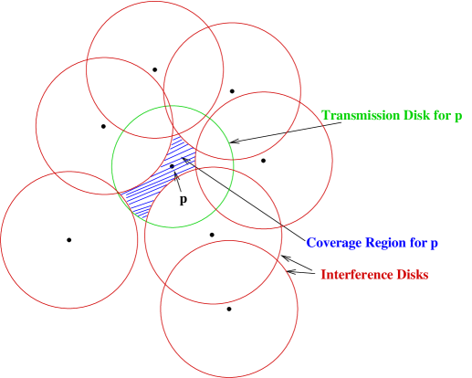
Figure 3.1: Coverage Region of a Transmitter

3.2 Our Approach

We show that for an appropriate choice of distance measure, coverage at each point can be computed by considering only certain nearby transmitters. The distance measure imposes a partition of the plane which our algorithm uses to compute the coverage map efficiently.

For equal ranges, the partition corresponds to the division of the plane into cells or Voronoi regions in the well-known closest point Voronoi Diagram[6]. For unequal ranges, we use a closely related structure called the Power Diagram. The partition by a power diagram is very similar in shape, structure, representation, and properties to the Voronoi Diagram[5].

The Voronoi Diagram (see, for example Figure 3.2) of a given set of points $T$ in 2-D partitions the plane into Voronoi regions - each point $p\in T$ corresponds to one region $\triangle(p,T)$. Every point in $\triangle(p,T)$ is closer, in Euclidean distance, to $p$ than to any other point in $T$.

Aurenhammer et al. [6] give a detailed treatment of the Voronoi Diagram, its properties and algorithms for its construction.

Figure 3.2: Voronoi Diagram of 8 Points

Two key claims to justify our approach -

Claim 3.1: The coverage region for a transmitter lies entirely in its Voronoi (or power) cell.

Claim 3.2: The Voronoi (or power) cell can be further partitioned such that coverage in each (sub-)partition can be decided by considering interference from only the nearest transmitter.

We develop our arguments starting with equal ranges and Voronoi diagrams, and later extend these to unequal ranges and power diagrams.

3.3 Equal Ranges and the Voronoi Diagram

We propose an augmentation to the Voronoi diagram of the point set corresponding to transmitter locations. This augmentation yields an efficient algorithm for computing the coverage map.

Let $T$ be the set of transmitter locations, and let $\mathbb{V}(T)$ denote their Voronoi diagram. Voronoi diagrams are classically used for reasoning about point sets. We show that we can apply Voronoi diagrams to our problem concerning interference disks with equal radii.

Let $\bigcirc(c,r)$ be a disk with center at $c$ and radius $r$. We write $\bigcirc$ when the parameters $c$ and $r$ are clear from the context. We define $\delta$, a signed distance measure between a point and a disk, as follows: $\delta(x,\bigcirc(c,r))=d(x,c)-r$, where $d(x,c)$ denotes the Euclidean distance between points $x$ and $c$. $\delta$ is a signed distance, since it is negative if $x\in\bigcirc$ and non-negative otherwise.

Observation 3.1.

Let $\bigcirc_{1}(c_{1},r)$ and $\bigcirc_{2}(c_{2},r)$ be two disks of equal radii, $r$, with centers $c_{1}$ and $c_{2}$ respectively. For a given point $x$, let $\delta_{1}$ and $\delta_{2}$ be the signed distances of $x$ from $\bigcirc_{1}$ and $\bigcirc_{2}$, respectively. $x$ is equidistant from the centers $c_{1}$ and $c_{2}$ if, and only if, $\delta_{1}=\delta_{2}$.

Proof.

$\delta_{1}=\delta_{2}\Leftrightarrow d(x,c_{1})-r=d(x,c_{2})-r$
$\Leftrightarrow d(x,c_{1})=d(x,c_{2})$ ∎

Similarly,

$$\delta(x,\bigcirc(c,r))>\delta(y,\bigcirc(c,r))\Leftrightarrow d(x,c)>d(y,c)$$

We make an observation that relates the distance measure to interference disks.

Observation 3.2.

Consider a point $x$ on the interference disk for $p$. $x$ is also on the interference disk of every transmitter closer than $p$.

Proof.

Let $q\in T\setminus\{p\}$. Let $x$ be closer to $q$ than $p$. Let $\bigcirc_{p}$ and $\bigcirc_{q}$ be the interference disks of $p$ and $q$, respectively.

Since $d(x,q)<d(x,p)\Rightarrow\delta(x,\bigcirc_{q})<\delta(x,\bigcirc_{p})$, if $x$ is in the interference range of $p$, $\delta(x,\bigcirc_{p})<0$. Which means that $\delta(x,\bigcirc_{q})<0$, i.e. $x$ must also be in the interference range of $q$. ∎

The Voronoi diagram of the centers of disks tells us which center is closest to a given point, in Euclidean distance. Given disks with equal radii, let us have a diagram which partitions points in the plane according to the disk nearest to them by the distance measure $\delta$; i.e. a ‘Voronoi’ diagram of disks. The above Observation 3.1 shows that the ‘Voronoi’ diagram of disks of equal radii using the signed distance measure $\delta$ is the same as the Voronoi diagram of the centers of the respective disks. Thus we can compute the classical Voronoi diagram, using the Euclidean distance measure, instead of the signed distances $\delta$. The ensuing discussion in this section thus refers directly to the Voronoi diagram of the transmitter locations and Euclidean point distances from them.

We now state notation and expressions for the points corresponding to a Voronoi region, its extreme points, and the Voronoi diagram.

The Voronoi region corresponding to a point $p\in T$ is given by:

$$\triangle(p)=\{x\ |\ d(x,p)<d(x,q),\forall q\in T\setminus\{p\}\}$$

The extreme points of the Voronoi region for $p$ are given by:

$$\partial(p)=\{x\ |\ d(x,p)\leq d(x,q),\forall q\in T\setminus\{p\}\}\setminus\triangle(p)$$

The Voronoi diagram is given by:

$$\mathbb{V}(T)=\displaystyle\bigcup_{p\in T}\partial(p)$$

We now prove an important property of the Voronoi region - it shows that the coverage region for a transmitter is confined to that transmitter’s Voronoi region.

Lemma 3.1 (Coverage in Voronoi Region).

Consider a point $x$ outside $\triangle(p)$ that is on the transmission disk for $p$. $x$ is also on some interference disk other than that of $p$.

Proof.

Let $q\in T\setminus\{p\}$, and $x\in\triangle(q)$. The Voronoi property implies that $p$ is farther away from $x$ than $q$. The transmission disk of $p$ is a subset of its interference disk; thus $x$ lies on the interference disk of $p$. Hence, by Observation 3.2, since $x$ is in the interference range of $p$, $x$ must also be in the interference range of $q$. ∎

Extreme points of $\triangle(p)$ appear as either Voronoi edges or vertices. These in turn correspond to some other transmitters in $T$ that we call the set of Voronoi neighbors of $p$, denoted by $\Gamma(p)$. Lets assume that the Voronoi diagram for $T$ has been built by some classical algorithm (see [6]). Suppose we delete the point $p$ from $T$, and build $\mathbb{V}(T\setminus\{p\})$. Figure 3.3 shows the effect of these changes. :

1. Some existing edges are extended - see dotted portions in Figure 3.3

2. Some existing edges are deleted - see dashed edges in Figure 3.3

3. Some new vertices are added - see intersections of dotted extensions in Figure 3.3

4. Some new edges are added - see edges between new vertices in Figure 3.3

Note that in figure 3.3, only the neighborhood of $p$ changes to form $\mathbb{V}(T\setminus\{p\})$. We will formally show later, in Lemma 3.2, that this is true for every Voronoi diagram.

Figure 3.3: Effect of deleting p

We call the new set of vertices, edges, and extension edges the Voronoi Frame corresponding to $p$. The dotted portions in Figure 3.3 are the Voronoi Frame. Edges in the frame correspond to the set of points equidistant from two transmitters adjacent to $p$ in $\mathbb{V}(T)$. Vertices in the frame correspond to points equidistant from three (or more) transmitters adjacent to $p$.

Before we delve into our discussion, we define certain terms in the context of what has been said so far.

Feasible Coverage Map: For a given transmitter $p$, this is the set of points lying in the Voronoi region of $p$, but outside every interference disk other than $p$. We reiterate that due to Lemma 3.1, to compute coverage, we can restrict our attention only to the Voronoi region of $p$.

Actual Coverage Map: For a given transmitter $p$, this is the set of points that lie in its Feasible Coverage Map and also on its transmission disk. The Actual Coverage Map of $p$ is the intersection of the transmission disk of $p$ with the Feasible Coverage Map. An Actual Coverage Area is demarcated by arcs, each of which correspond to the portion of the periphery of either the transmission disk of $p$, or an interference disk of a Voronoi neighbor of $p$ that bounds the Feasible Coverage Map.

Contiguous Feasible Region: The Feasible Coverage Map may be composed of several disjoint maximal simply-connected subsets (see, for example, the two shaded sets in figure 3.5). These subsets are called Contiguous Feasible Regions. In the subsequent text we use the term ‘Feasible Region’ when the word ‘Contiguous’ is obvious from the context.

Voronoi Frame: For a given transmitter $p$, this is the set of points on extension edges, new edges and vertices in $\triangle(p)$ obtained from deleting the point $p$ and adding new extreme points from the Voronoi diagram of $T\setminus\{p\}$. The only extreme points in $\mathbb{V}(T)$ that do not belong in $\mathbb{V}(T\setminus\{p\})$ are the extreme points on the edges in $\triangle(p)$. The Voronoi Frame is thus the set of points in $\mathbb{V}(T\setminus\{p\})\setminus\mathbb{V}(T)$.

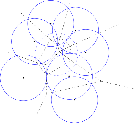
Figure 3.4: Feasible Coverage Map: Closed Feasible Region

Figure 3.5: Feasible Coverage Map: Multiple Contiguous Feasible Regions

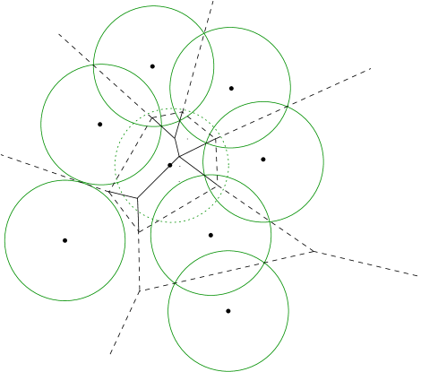
Figure 3.6: Feasible Coverage Map: Open Feasible Region

Our goal in this remainder of this section is to demonstrate how the Voronoi Frame aids in reasoning about the Feasible and Actual Coverage Maps.

Figures 3.4, 3.5, and 3.6 will help the reader visualize the concepts being discussed. Each figure corresponds to the same set of transmitter locations. The interference radii, however, are different.

1. Interference disks are shown with solid perimeters.

2. Only one transmission disk is shown. It is shown by a dotted perimeter.

3. The original Voronoi diagram is shown by dashed lines.

4. The Voronoi Frame is shown by solid lines.

5. Figure 3.4 illustrates a closed Feasible Region; i.e. one that is bounded on all sides by interference disks.

6. Figure 3.5 illustrates two Contiguous Feasible Regions in one Feasible Coverage Map.

7. Figure 3.6 illustrates an open Feasible Region.

We now show that only neighbors of $p$ in $\mathbb{V}(T)$ contribute edges in the Voronoi Frame for $p$. We actually observe a more general result - that all points in a Voronoi region are closer to Voronoi neighbors than to any other point -

Lemma 3.2.

Let $x\in\triangle(p)$. The closest point to $x$ in $T\setminus\{p\}$ is a Voronoi neighbor of $p$ in $\mathbb{V}(T)$.

Proof.

Let $q$ be the closest point to $x$ in $T\setminus\{p\}$. Assume that $q$ is not a neighbor of $p$. We show that this leads to a contradiction. Note that $p$ and $q$ have distinct Voronoi regions, and each of them is a partition of the plane. Thus the line segment joining $x$ and $q$ must intersect an edge of $\partial(p)$. Let this intersection point be $x_{0}$, and the Voronoi neighbor of $p$ on this edge be $q_{0}$. The position of the points is shown in figure 3.7.

Since $p$ and $q_{0}$ are neighbors, $d(x_{0},p)=d(x_{0},q_{0})$
$\Rightarrow$ {Since $p$ and $q$ are not neighbors, } $d(x_{0},q)>d(x_{0},p)$
$\Rightarrow$ {Adding $d(x,x_{0})$ to both sides, } $d(x,x_{0})+d(x_{0},q)=d(x,q)>d(x,x_{0})+d(x_{0},q_{0})$
$\Rightarrow$ {Since $x$, $x_{0}$, and $q$ are collinear, } $d(x,q)>d(x,x_{0})+d(x_{0},q_{0})$
$\Rightarrow$ {By the triangle inequality, } $d(x,x_{0})+d(x_{0},q_{0})\geq d(x,q_{0})$
$\Rightarrow d(x,q)>d(x,q_{0})$
This contradicts the assumption that $q$ is the closest point to $x$ in $T\setminus\{p\}$. ∎

Figure 3.7: Illustration of Lemma 3.2

Corollary 3.3.

If a point $x\in\triangle(p)$ is in the interference range of some transmitter $t\neq p$, it is in the interference range of a neighbor of $p$.

Proof.

Lemma 3.2 states that the closest point to $x$ in $T\setminus\{p\}$ is a neighbor of $p$. Thus, using Observation 3.2 we infer that $x$ is in the interference range of a neighbor of $p$. ∎

We denote by $\nu(x,S)$ the set of points in $S$ closest to $x$. We can now give an expression for the Voronoi Frame corresponding to $p$. Due to Corollary 3.3, the Voronoi Frame has edges only from Voronoi neighbors :

$$\bot(p)=\{x\in\triangle(p)\ |\ \exists\{q_{1},q_{2}\}\subseteq\nu(x,\Gamma(p))\}$$

Our aim is to compute the Actual Coverage Map for $p$. We will use the Voronoi Frame of $p$ to do so. Note that not all points on the Voronoi Frame are in the Feasible Coverage Map. This is because some interference disk corresponding to a neighbor may include part of an edge on the Voronoi Frame. Our first task is to exclude points on the Voronoi Frame that are on some interference disk in $T\setminus\{p\}$. We call the resultant subset of the Voronoi Frame the Feasible Coverage Frame. Corollary 3.3 shows that to obtain the Feasible Coverage Frame it is sufficient to exclude points on interference disks adjacent to edges in the Voronoi Frame. For each edge in the frame, we remove the portion of the edge on one of its adjacent interference disks. This results in zero, one, or two corresponding edges - depending on whether the edge has no points in any Feasible Coverage Region, is partially in a Feasible Coverage Region, or is entirely in a Feasible Coverage Region. We illustrate this operation in figure 3.8.

Figure 3.8: Voronoi Frame Yields Feasible Coverage Frame

Definition 3.1 (Feasible Coverage Frame).

For a given transmitter $p$, this is the set of points that lie on its Voronoi Frame and outside the union of interference disks of its neighbors.

Formally, the Feasible Coverage Frame for transmitter $p$ is given as:

$$\bot_{g}(p)=\bot(p)\setminus\{x\ :\ x\in\bigcirc^{i}(q),\forall q\in\Gamma(p)\}$$

where $\bigcirc^{i}(q)$ denotes the interference range of the transmitter at $q$.

We now have a procedure for building a Voronoi Frame for a transmitter, and for using this Voronoi Frame to find the transmitter’s Feasible Coverage Frame. We note a property of the Voronoi Frame that we will use to show its correlation with the Feasible Coverage Region.

Observation 3.3.

$\bot(p)$ partitions $\triangle(p)$, and each partition corresponds to exactly one neighbor in $\Gamma(p)$.

Proof.

$\mathbb{V}(T\setminus\{p\})$, due to the Voronoi property, partitions the plane. By definition, the Voronoi Frame is the subset of this Voronoi diagram lying inside $\triangle(p)$. Hence $\triangle(p)$ is partitioned by the Voronoi Frame. Each point in a partition belongs to some Voronoi region in $\mathbb{V}(T\setminus\{p\})$. Due to Lemma 3.2, a point in such a partition can be closest only to a neighbor of $p$ in $\mathbb{V}(T)$.

Each point in a partition can, by definition, be closest only to one point in $T\setminus\{p\}$. Hence, the partition corresponds to exactly one neighbor. ∎

Note that the edges in the Voronoi Frame bounding this partition correspond to the edges contributed by a neighbor of $p$. Further, since $p$ is closer than $q$ to each point in this partition, the edge between $p$ and $q$ also bounds the partition.

This observation is illustrated by figure 3.9. We denote by $\blacktriangle(p,q)$ the partition of $\triangle(p)$ by edges on the Voronoi Frame corresponding to $q$. Formally,

$$\blacktriangle(p,q)=\triangle(p)\cap\{x\ |\ q\in\nu(x,\Gamma(p))\}$$

Figure 3.9: Voronoi Frame Partitions Voronoi Region

We note a correlation between $\blacktriangle(p,q)$ and the interference disk for $q$.

Corollary 3.4.

If $x\in\blacktriangle(p,q)$ and $x$ is in the interference range of some transmitter $t\neq p$, then $x$ is in the interference range of $q$.

Proof.

By definition, every point in $\blacktriangle(p,q)$ is closer to $q$ than any other point in $T$. Since $x$ is closer to $q$ than $t$, we can apply Observation 3.2 to see that $x$ is in the interference range of $q$. ∎

We refer again to figures 3.4, 3.5, and 3.6. We observe that each Contiguous Feasible Region is bounded by the arcs of the rims of interference disks. These disks correspond to edges in the Feasible Coverage Frame enclosed within the Feasible Region.

We could compute the Actual Coverage Map of a transmitter directly by intersections of each Contiguous Feasible Region with the transmission disk. This would get us the coverage map. However, this would require our algorithm to represent the Contiguous Feasible Region as a sequence of arcs. Instead, we obtain the Actual Coverage Map by an alternative approach that uses the Voronoi properties.

We denote the Actual Coverage Map of a transmitter $p$ by $\chi(p)$. The following result shows that the partition given by the Voronoi Frame allows us to compute the coverage map by excluding interference from just neighboring transmitters.

Theorem 3.5 (Transmitter’s coverage map can be computed by excluding interference only from Voronoi neighbors).

$$\chi(p)=\bigcup_{q\in\Gamma(p)}(\bigcirc^{t}(p)\cap\blacktriangle(p,q))\setminus\bigcirc^{i}(q)$$

Proof.

Let $\bigcirc^{i}(p)$ and $\bigcirc^{t}(p)$ denote the interference and transmission disks, respectively, of transmitter $p$. Lemma 3.1 implies that the Actual Coverage Map lies inside $\triangle(p)$. Also, Observation 3.3 states that the Contiguous Feasible Region for $p$ is composed of contributions from each neighbor. Corollary 3.4 shows that to find points within $\blacktriangle(p,q)$ that lie in the Feasible Coverage Map, it is sufficient only to exclude points on the interference disk of $q$. Thus the Actual Coverage Area can be computed from the individual regions contributed by each partition. ∎

The advantage of using the Voronoi Frame is now clear - we need only the Feasible Frame to represent the Actual Coverage Map. Also, to compute the Actual Coverage Map, only two arc intersection computations are required for each neighbor $q$ - one for $\bigcirc^{t}(p)$, and one for $\bigcirc^{i}(q)$.

In order to compute $\chi(p)$ we need a generalized polygon representation that allows circular arcs as edges. Berberich et al. [27] study intersections of polygons with arcs. We defer discussion on these generalized polygons until Section 3.5.

In this section we have shown how to compute the coverage map for a set of transmitters having the same interference (and transmission, respectively) radius. We generalize the arguments presented here to transmitters with unequal interference (and transmission, respectively) radii in Section 3.4.

3.4 Unequal Ranges and the Power Diagram

Note that Observation 3.1 does not hold when the interference radii (and transmission radii, respectively) are not the same. This is because equal minimum Euclidean distance of point $x$ from two disks $\bigcirc(c_{1},r_{1})$ and $\bigcirc(c_{2},r_{2})$, where $r_{1}\neq r_{2}$ does not imply equal Euclidean distance of the centers $c_{1}$ and $c_{2}$ from $x$. Thus, we need find an alternative distance measure.

The Voronoi Diagram of the centers of disks tells us which center is closest to a given point, in Euclidean distance. The Power Diagram (see Aurenhammer et al. [5]) is a generalization of the Voronoi Diagram; and is based on a different distance measure (between a point and a disk), called the Power Distance. We denote the power distance by $\rho$.

The power distance of a point $x$ from a disk $\bigcirc$ of radius $r$ and center $c$ is defined by $\rho(x,\bigcirc)=d(x,c)^{2}-r^{2}$; where $d(x,c)$ is the Euclidean distance between $p$ and the center $c$. Geometrically, the power distance of a point outside a disk is the square of the length of the tangent from that point to the disk rim. Inside the disk perimeter, the power Distance is negative in sign, and corresponds to the square of half the length of the chord normal to the line joining the point and the center of the disk.

Figure 3.10 shows a power diagram of 7 disks in the plane. Some fundamental properties of the power diagram are stated in [5]. The power diagram for $\Psi$, a set of disks, partitions the plane into convex polygonal regions, i.e. shapes exactly like Voronoi regions. A point lies in the Power Region corresponding to disk $\bigcirc\in\Psi$ if its power distance from $\bigcirc$ is less than its power distance from every other disk in $\Psi$.

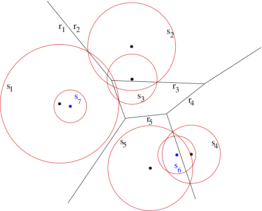
Figure 3.10: Power Diagram: 7 disks, 5 regions (adapted from [5])

The power diagram for disks with equal radii (under distance measure $\rho$) is a Voronoi diagram (under Euclidean distance measure $d(p,c)$.) The generalization, however, leads to instances where a disk does not have a corresponding power region. One such instance is shown in figure 3.10. There are no power regions corresponding to disks $s_{6}$ and $s_{7}$; since no point in the plane is closest (by $\rho$) to any of these disks. In this chapter we assume that every disk has a corresponding power region. We discuss the impact of relaxing this assumption later in Chapter 4.

The power diagram generalizes the Voronoi distance measure of $\delta$ to $\rho$. This leads us to three key facts, which together form the core of our progression from Voronoi diagrams to power diagrams as tools for computing the coverage map.

1. A generalization of Observation 3.2 shows the same relationship exists between the power region and interference disks. This generalization is shown in Observation 3.4.

2. A generalization of Lemma 3.1 (Lemma 3.6 also holds when the distance measure is replaced by $\rho$. This means that the Actual Coverage Map will lie only in the power region.

3. A generalization of Lemma 3.2 is also possible, as we will see shortly in Lemma 3.7. This means that we need to consider interference only from transmitters that are Power Neighbors.

In Table 3.1, we introduce the new notation for unequal ranges and the power diagram. We also note the corresponding notation with equal ranges and the Voronoi diagram.

Equal Ranges	Unequal Ranges
Voronoi Diagram $\mathbb{V}(T)$	Power Diagram $\mathbb{P}(T)$
Transmitter Location $p$	Transmitter Location $\tilde{p}$
Voronoi Region $\triangle(p)$	Power Region $\triangle(\tilde{p})$
Voronoi Neighbors $\Gamma(p)$	Power Neighbors $\Gamma(\tilde{p})$
Voronoi Frame $\bot(p)$	Power Frame $\bot(\tilde{p})$
Voronoi Region partition by Voronoi Frame $\blacktriangle(p,q)$	Power Region partition by Power Frame $\blacktriangle(\tilde{p},\tilde{q})$

Table 3.1: Notation for Unequal Ranges

We begin with an observation that relates the distance measure $\rho$ to interference disks. Note its correspondence with Observation 3.2

Observation 3.4.

Consider a point $x$ on the interference disk for $\tilde{p}$. $x$ is also on the interference disk of every transmitter closer than $\tilde{p}$ in power distance.

Proof.

Let $\tilde{q}\in T\setminus\{\tilde{p}\}$. Let $x$ be closer, by power distance measure $\rho$, to $\tilde{q}$ than $\tilde{p}$. Let $\bigcirc_{\tilde{p}}$ and $\bigcirc_{\tilde{q}}$ be the interference disks of $\tilde{p}$ and $\tilde{q}$, respectively.

Since $\rho(x,\bigcirc_{\tilde{q}})<\rho(x,\bigcirc_{\tilde{p}})$, if $x$ is in the interference range of $\tilde{p}$, $\rho(x,\tilde{p})<0$. Which means that $\rho(x,\tilde{q})<0$, i.e. $x$ must also be in the interference range of $\tilde{q}$. ∎

We now observe the following generalization of Lemma 3.1 -

Lemma 3.6 (Coverage in Power Region).

Consider a point $x$ outside $\triangle(\tilde{p})$ that is on the transmission disk for $\tilde{p}$. $x$ is also on some interference disk other than that of $\tilde{p}$.

Proof.

Let $\tilde{q}\in T\setminus\{\tilde{p}\}$, and $x\in\triangle(\tilde{q})$. Since the power diagram is a partition of the plane, such a $\tilde{q}$ exists. Thus, $x$ is closer to $\tilde{q}$, in power distance, than it is to $\tilde{p}$. The transmission disk of $\tilde{p}$ is a subset of its interference disk; thus $x$ lies on the interference disk of $\tilde{p}$. Hence, by Observation 3.4 $x$ must also be on the interference disk of $\tilde{q}$. ∎

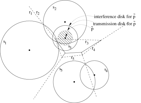
Figure 3.11: Power Diagram with Power Frame

In the ensuing discussion, we will implicitly assume the use of the distance measure $\rho$, the power distance; that is, we will say ‘closest’ or ‘closer’ (respectively, ‘farthest’ or ‘farther’) to mean closest or closer (farther, farthest, respectively) in power distance.

Lemma 3.7.

Assume that every transmitter has a non-empty power region. Let $x$ be a point in the power region of transmitter $\tilde{p}$, i.e. $\triangle(\tilde{p})$. If $\tilde{q}$ is the closest (by power distance) transmitter in $T\setminus\{\tilde{p}\}$ to $x$, then $\tilde{q}$ is a power neighbor of $\tilde{p}$.

Proof.

We denote by $\triangle(\tilde{p},T)$ the power region of $\tilde{p}$ in the power diagram of the set of transmitters $T$. Similarly, $\triangle(\tilde{q},T\setminus\{\tilde{p}\})$ denotes the power region of $\tilde{q}$ in the set of transmitters $T\setminus\{\tilde{p}\}$. By definition, $x\in\triangle(\tilde{p},T)\cap\triangle(\tilde{q},T\setminus\{\tilde{p}\})$.

Assume that $\tilde{q}$ is not a power neighbor of $\tilde{p}$. We show that this leads to a contradiction.

Case 1 : Assume that an extreme point $x_{0}$ of $\triangle(\tilde{p},T)$ lies in $\triangle(\tilde{q},T\setminus\{\tilde{p}\})$. We show that this leads to a contradiction.

Let $\tilde{q_{0}}$ be a power neighbor of $\tilde{p}$ corresponding to the point $x_{0}$. Thus,

$$\rho(x_{0},\tilde{p})=\rho(x_{0},\tilde{q_{0}})$$

However, since $\tilde{q}$ is closer to $x_{0}$ than $\tilde{q_{0}}$,

$$\rho(x_{0},\tilde{p})=\rho(x_{0},q_{0})>\rho(x_{0},\tilde{q})$$

This is a contradiction since no transmitter can be closer to $x_{0}$ than $\tilde{p}$. Thus, no extreme points of $\triangle(\tilde{p},T)$ lie in $\triangle(\tilde{q},T\setminus\{\tilde{p\}})$.

Case 2 : Assume that no extreme point of $\triangle(\tilde{p},T)$ lies in $\triangle(\tilde{q},T\setminus\{\tilde{p}\})$. We show that this leads to a contradiction.

$\Rightarrow$ All edges in $\triangle(\tilde{p},T)$ lie outside $\triangle(\tilde{q},T\setminus\{\tilde{p}\})$.
$\Rightarrow$ Either $\triangle(\tilde{q},T\setminus\{\tilde{p}\})\subset\triangle(\tilde{p},T)$, or $\triangle(\tilde{q},T\setminus\{\tilde{p}\})\cap\triangle(\tilde{q},T\setminus\{\tilde{p}\})=\phi$.
In other words, the power region of $\tilde{p}$ in $\mathbb{P}(T)$ either encloses that of $\tilde{q}$ in $\mathbb{P}(T\setminus\tilde{p})$, or the two power regions are disjoint.
Since $x\in\triangle(\tilde{p},T)\cap\triangle(\tilde{q},T\setminus\{\tilde{p}\})\Rightarrow\triangle(\tilde{p},T)\cap\triangle(\tilde{q},T\setminus\{\tilde{p}\})\neq\phi$
Thus, $\triangle(\tilde{q},T\setminus\{\tilde{p}\})\subset\triangle(\tilde{p},T)$
$\Rightarrow$ each point in $\triangle(\tilde{q},T\setminus\{\tilde{p}\})$ is closer to $\tilde{p}$ than $\tilde{q}$.
$\Rightarrow\triangle(\tilde{q},T)=\phi$
This contradicts the assumption that no power region is empty.∎

Having established the basic correspondence between Voronoi diagrams and power diagrams, we note that Observation 3.3, Corollary 3.4, and Theorem 3.5 are directly applicable to power diagrams. We give corresponding results next.

Observation 3.5.

$\bot(\tilde{p})$ partitions $\triangle(\tilde{p})$, and each partition corresponds to exactly one neighbor in $\Gamma(\tilde{p})$.

Proof.

$\mathbb{P}(T\setminus\{\tilde{p}\})$, by definition, partitions the plane. By definition, the power frame is the subset of this power diagram lying inside $\triangle(\tilde{p})$. Hence $\triangle(\tilde{p})$ is partitioned by the power frame. Each point in a partition belongs to some power region in $\mathbb{P}(T\setminus\{\tilde{p}\})$. Due to Lemma 3.7, a point in such a partition can be closest only to a neighbor of $\tilde{p}$ in $\mathbb{P}(T)$.

Each point in a partition can, by definition, be closest only to one point in $T\setminus\{\tilde{p}\}$. Hence, the partition corresponds to exactly one neighbor. ∎

We note that the same relationship as Corollary 3.4 holds between $\blacktriangle(\tilde{p},\tilde{q})$ and the interference disk for $\tilde{q}$.

Corollary 3.8.

If $x\in\blacktriangle(\tilde{p},\tilde{q})$ and $x$ is in the interference range of some transmitter $\tilde{t}\neq\tilde{p}$, then $x$ is in the interference range of $\tilde{q}$.

Proof.

By definition, every point in $\blacktriangle(\tilde{p},\tilde{q})$ is closer to $\tilde{q}$ than any other point in $T$. Since $x$ is closer to $\tilde{q}$ than $\tilde{t}$, we can apply Observation 3.4 to see that $x$ is in the interference range of $\tilde{q}$. ∎

We now state and prove our main theorem. Note that it is a generalization of Theorem 3.5.

We denote the Actual Coverage Map of a transmitter $\tilde{p}$ by $\chi(\tilde{p})$. The following result shows that, if no power region is empty, then the partition given by the power frame allows us to compute the coverage map by excluding interference from just one transmitter.

Theorem 3.9.

Assume no power region is empty. Then,

$$\chi(\tilde{p})=\bigcup_{q\in\Gamma(\tilde{p})}(\bigcirc^{t}(\tilde{p})\cap\blacktriangle(\tilde{p},\tilde{q}))\setminus\bigcirc^{i}(\tilde{q})$$

Proof.

Let $\bigcirc^{i}(\tilde{p})$ and $\bigcirc^{t}(\tilde{p})$ denote the interference and transmission disks, respectively, of transmitter $\tilde{p}$. Since no power region is empty, Lemma 3.6 implies that the Actual Coverage Map lies inside $\triangle(\tilde{p})$. Also, Observation 3.5 states that the Contiguous Feasible Region for $\tilde{p}$ is composed of contributions from each neighbor. Corollary 3.8 shows that to find points within $\blacktriangle(\tilde{p},\tilde{q})$ that lie in the Feasible Coverage Map, it is sufficient only to exclude points on the interference disk of $\tilde{q}$. Thus the Actual Coverage Map can be computed from the individual regions contributed by each partition. ∎

3.4.1 Removing Redundant Transmitters

The power region corresponding to a circle may be empty - as is the case with $s_{7}$ in figure 3.10. No point on the power bisector of $s_{1}$ and $s_{7}$ appears in the power diagram since each point on this bisector is closer to either $s_{2}$, $s_{3}$, or $s_{5}$.

However, as we will show below, if a disk $\bigcirc$ has an empty power region then it is included in the union of other disks in $\Psi$. A disk that belongs in the union of other disks has an empty coverage map, since every point on it is in the interference range of some other transmitter. Hence, for our purposes, during preprocessing we can remove disks that do not have a corresponding power region.

We show a more general result - that if a disk and its corresponding power region have no points in common, then that disk is included in the union of other disks.

Lemma 3.10 (Empty Power Regions).

Let $\tilde{q}$ be a transmitter with interference disk $\bigcirc_{\tilde{q}}$, such that $\bigcirc_{\tilde{q}}\cap\triangle(\tilde{q})=\phi$. Then,

$$\bigcirc_{\tilde{q}}\subseteq\bigcup_{\tilde{p}\in T\setminus\tilde{q}}\bigcirc_{\tilde{p}}$$

Proof.

We prove this result by contradiction.

Let $\bigcirc_{\tilde{q}}\nsubseteq\displaystyle\bigcup_{\tilde{p}\in T\setminus\tilde{q}}\bigcirc_{\tilde{p}}$
$\Rightarrow\exists x\in\bigcirc_{\tilde{q}}$ such that $\forall\tilde{p}\neq\tilde{q},\ x\notin\bigcirc_{\tilde{p}}$
$\Rightarrow(\rho(x,\bigcirc_{\tilde{q}})<0)\land(\forall\tilde{p}\neq\tilde{q},\ \rho(x,\bigcirc_{\tilde{q}})>0)$
$\Rightarrow x\in\triangle(\tilde{q})$
$\Rightarrow x\in\triangle(\tilde{q})\cap\bigcirc_{\tilde{q}}$
This contradicts the assumption that $\triangle(\tilde{q})\cap\bigcirc_{\tilde{q}}$ is empty. ∎

This fact justifies our pre-processing step for removing disks that have an empty power region.

3.5 Algorithm

We collate the observations made in the preceding text into an algorithm. The inputs to the algorithm are: a set $T$ of transmitters, their locations in the plane, and their transmission and interference radii. The algorithm outputs a coverage map for $T$, denoted by $\widehat{\chi}(T)$.

Notation defined in Table 3.1 is used in the algorithm. In addition, we denote by $\hbar(\tilde{p},\tilde{q})$ the half-space of points closer to $\tilde{p}$ than $\tilde{q}$.

Algorithm 3.1 (Coverage Map).

1. Initialize: $\widehat{\chi}(T)\leftarrow\phi$.

2. Compute the Power Diagram $\mathbb{P}(T)$.

3. For each transmitter $\tilde{p}\in T$, do If $\triangle(\tilde{p})=\phi$, $T\leftarrow T\setminus\{\tilde{p}\}$.

4. For each transmitter $\tilde{p}\in T$, do

   1. $\chi(\tilde{p})\leftarrow\phi$

   2. Find the Power Diagram of $\Gamma(\tilde{p})$, i.e.$\mathbb{P}(\Gamma(\tilde{p}))$.

   3. For each region $\triangle(\tilde{q},\Gamma(\tilde{p}))$, do

      1. $\blacktriangle(\tilde{p},\tilde{q})\leftarrow\triangle(\tilde{q},\Gamma(\tilde{p}))\cap\hbar(\tilde{p},\tilde{q})$

      2. $\chi(\tilde{p})\leftarrow\chi(\tilde{p})\cup((\blacktriangle(\tilde{p},\tilde{q})\cap\bigcirc^{t}_{\tilde{p}})\setminus\bigcirc^{i}_{\tilde{q}})$

5. For each transmitter $\tilde{p}\in T$, do $\widehat{\chi}(T)\leftarrow\widehat{\chi}(T)\cup\chi(\tilde{p})$

3.5.1 Running Time Analysis

We show a proof sketch of a result from Aurenhammer et al. [5] that bounds the number of power edges in a power diagram.

Observation 3.6.

The number of power edges in a power diagram is less than $3n-6$.

Proof.

The power diagram in the plane is a planar graph. Its dual graph $D(\mathbb{P})$ contains exactly one vertex for each region of $\mathbb{P}$. Two vertices of $D(\mathbb{P})$ are connected by an edge if, and only if, the boundaries of the corresponding regions of $\mathbb{P}$ have an edge in common. $D(\mathbb{P})$ is a triangulation on $n$ vertices. A triangulation on $n$ vertices cannot have more than $3n-6$ edges. ∎

We make an observation that the sum of the number of neighbors over all transmitters is linear in $n$. This result will be invoked in our proof.

Observation 3.7 (Sum of Neighbors).

$$\sum_{\tilde{p}\in T}|\Gamma(\tilde{p})|=O(n)$$

Proof.

The sum $\displaystyle\sum_{\tilde{p}\in T}|\Gamma(\tilde{p})|$ is also the number of ordered pairs $(\tilde{p},\tilde{q})$ such that $\tilde{p}$ and $\tilde{q}$ are neighbors in $\mathbb{P}(T)$. Since each power edge in $\mathbb{P}(T)$ corresponds to two transmitters, the latter is twice the number of power edges, which is $O(n)$ by Observation 3.6 ∎

Theorem 3.11 (Runtime).

The coverage map of ‘$n$’ transmitters with equal or unequal ranges can be constructed in $O(n\log{n})$ time.

Proof.

Step 2 A power diagram of $n$ disks in the plane can be constructed in $O(n\log{n})$ time (see [4]).

Step 4b: The power diagram of $\Gamma(\tilde{p})$ can be constructed in $O(|\Gamma(\tilde{p})|\log{|\Gamma(\tilde{p})|}$ time. Now, $\log{|\Gamma(\tilde{p})|}\leq\log{n}$
$\Rightarrow\displaystyle\sum_{\tilde{p}\in T}|\Gamma(\tilde{p})|\log{|\Gamma(\tilde{p})|}\leq(\log{n})\sum_{\tilde{p}\in T}|\Gamma(\tilde{p})|$
$\Rightarrow$ {By Observation 3.7} $(\log{n})\displaystyle\sum_{\tilde{p}\in T}|\Gamma(\tilde{p})|=O(n\log{n})$
The total time to compute the power diagrams for all transmitters is thus $O(n\log{n})$.

Step 4(c)i: A well-known algorithm (see [28]) for convex polygon intersection can be used to compute the partition. This algorithm is linear in the total number of edges, i.e. in our case $O(|\Gamma(\tilde{p})|)$. By Observation 3.7, the total time taken executing this step is $O(n)$.

Step 4(c)ii: The union and set difference operations can be performed by the sweep-line algorithm from [27]. This computation is also linear time in the number of line segments (edges) and arcs; i.e. in our case $O(|\Gamma(\tilde{p})|)$. By Observation 3.7, the total time taken executing this step is $O(n)$.

Step 4c: Each transmitter $\tilde{p}$ can contribute a partition only to a neighbor (Lemma 3.6). Thus the total number of partitions created by the algorithm is the sum of neighbors, which is $O(n)$ by Observation 3.7. Since each edge appears in at most two partitions, the total number of edges created in this step is also $O(n)$.

Hence, the coverage map can be computed in $O(n\log{n})$ time. ∎

3.6 A Lower Bound on Coverage Map Computation

We show here that $O(n\log{n})$ time is optimal in an algebraic decision- tree model. We use a result on the lower bound of the classical $\epsilon$- closeness problem to show that computing the coverage map is $\Omega(n\log{n})$. Our proof is adapted from the proof for the lower bound for constructing Voronoi diagrams by reduction from the $\epsilon$-closeness problem [6].

We first present a formal representation of the coverage map. We then use this representation to locate a transmitter with a certain property we call interference-bound. We show that this operation takes $O(n)$ time. We then reduce the $\epsilon$-closeness problem to that of computing the coverage map for a suitable set of transmitters and using it to locate an interference-bound transmitter. Given a coverage map, an interference-bound transmitter can be found in $O(n)$ time. Thus, if the coverage map can be constructed in $o(n\log{n})$ time, then $\epsilon$-closeness can be solved in $o(n\log{n})$ time as well. This reduction shows that constructing the coverage map is $\Omega(n\log{n})$.

3.6.1 A Representation of the Coverage Map

We represent the coverage map $\widehat{\chi}(T)$ as the union of all coverage regions for transmitters in $T$. Each coverage region is represented by a set of arc-polygons, each a list $(s_{1},s_{2}\ldots s_{k},s_{1})$ of $k$ circular arcs forming a connected closed chain.

Though not explicit in the representation, the areas enclosed by these chains form the coverage region. In a particular chain $(s_{1},s_{2}\ldots s_{k},s_{1})$, corresponding to transmitter $\tilde{p}$, there is at most one arc corresponding to the rim of the transmission disk for $\tilde{p}$ (curving outward), whereas the remaining arcs correspond to rims of interference disks of transmitters interfering with $\tilde{p}$ (curving inward).

3.6.2 Locating an Interference-Bound Transmitter

A transmitter whose transmission disk intersects with an interference disk of another transmitter is called interference-bound. Assume that such a transmitter $\tilde{p}$ exists and has a non-empty coverage region. The coverage region for $\tilde{p}$ has at least one inward arc - corresponding to a transmitter that intersects with its transmission disk.

Suppose we are given a coverage map $\widehat{\chi}(T)$, and we want to find whether there exists an interference-bound transmitter in $T$. We first test for a transmitter with an empty coverage region. We then test each arc in the coverage map to check that it is not a complete circle. Thus, given the coverage map, one can find an interference-bound transmitter in time linear in the number of arcs in the coverage map. We show that the number of arcs is $O(n)$.

Lemma 3.12.

If no power region is empty, then the total number of arcs in the coverage map is $O(n)$.

Proof.

We analyze using the partition of the power region by the power frame. Each neighboring pair of transmitters contributes to one partition each in two power regions (one for each neighbor in the pair). Thus, the total number of partitions is twice the sum of neighboring pairs, i.e $O(n)$. Each partition corresponds to at most one inward arc and at most one outward arc. Thus, the total number of arcs is also $O(n)$. ∎

Thus, given a coverage map for the above configuration, an interference-bound transmitter can be located in $O(n)$ time.

3.6.3 A reduction from the $\epsilon$-closeness problem

The lower bound for the $\epsilon$-closeness problem is a classical problem related to many fundamental proximity problems in computational geometry. We formally state the problem in Lemma 3.13 below.

Lemma 3.13 ($\epsilon$-closeness).

Consider a real number $\epsilon$ and a sequence $(a_{1},a_{2},\ldots,a_{n})$ of $n$ real numbers. Finding whether there exists a pair of real numbers $\{a_{i},a_{j}\}$ in this sequence such that $|a_{i}-a_{j}|<\epsilon$ is $\Omega(n\log{n})$.

Proof.

Refer Chapters 5 and 8 in Preparata et al. [29]. ∎

We now prove our main result by reducing the $\epsilon$-closeness problem to computing a coverage map.

Theorem 3.14.

The coverage map problem is $\Omega(n\log{n})$.

Proof.

The input given to the $\epsilon$-closeness problem is $\epsilon$ and the sequence of real numbers $(a_{1},a_{2},\ldots,$ $\ a_{n})$. Given this input we construct a set of $n$ transmitters as input for the coverage problem as follows - the center of transmitter $\tilde{p}_{i}$ is $(a_{i},0)$, the transmission radius of each transmitter is $\frac{\epsilon}{3}$, and the interference radius of each transmitter is $\frac{2\epsilon}{3}$.

Suppose we have the coverage map for this set of transmitters. A transmitter is interference-bound only if its transmission disk intersects with some other transmitter’s interference disk. Given our placement of the disks, this can occur only if there exists a pair of transmitters whose centers are located less than $\epsilon$ distance apart. The distance between two transmitters, however, is the same as the (unsigned) difference between the corresponding real numbers in the $\epsilon$-closeness problem. Hence, the existence of an interference-bound transmitter implies the existence of a pair $\{a_{i},a_{j}\}$ separated by distance less than $\epsilon$. Thus, the coverage map problem must be $\Omega(n\log{n})$. ∎

Chapter 4 Coverage in the Protocol Model: Dynamic Set of Transmitters

We consider two update operations - addition and deletion of one transmitter, and propose a method to maintain the coverage map efficiently on each update. Our purpose is to achieve efficiency comparable to the static algorithm in Chapter 3.

In this chapter we report a randomized algorithm whose efficiency is expressed as a sum of two components - expected and deterministic. The expected cost is an expectation over random choices made in building internal data structures - in other words, the expected cost of locating coverage regions affected by the update. This cost is $O(\log{n})$; independent of the sequence of updates. The other component is a deterministic cost. Lets say we have found $k$ disks whose power regions are affected by a particular update. Our algorithm updates the contours of the corresponding coverage regions in $O(k)$.

4.1 Our Approach

The key ideas we use in our approach are:

1. Dynamic maintenance of Power Diagrams

   1. Mapping from set of 2-D disks to a 3-D convex polytope This mapping is used for dynamic construction of Voronoi diagrams in Mulmuley [7, Chapters 3 and 4], following the original idea from Brown [30]. A similar map is used for static construction of power diagrams in Aurenhammer [5].

   2. Dynamic maintenance of a 3-D convex polytope We have chosen an algorithm from Mulmuley [7, Chapter 4]. We have adapted this algorithm to suit our purpose without compromising on its efficiency. This adaptation is discussed later in Section 4.4.

2. Dynamic maintenance of disk intersections We use the new power regions to update disk intersections efficiently.

In Section 4.2 we illustrate our ideas using dynamic 1-D Voronoi diagram maintenance as a conceptual tool. Later, in Section 4.3, we show how these ideas can be extended to 2-D power diagrams. Section 4.3 shows the use of the new power region to compute the new coverage regions. In Section 4.3 we also present an analysis of these algorithms. In Section 4.4, we present the use of the power frame to update disk intersections efficiently. Finally, in Section 4.5, we explore dynamic maintenance of the coverage map in presence of transmitters with empty power regions.

4.2 Dynamic 1-D Voronoi Diagrams

A Voronoi diagram of a set of points on the $x$-axis directly corresponds to the sorted sequence of these points, ordered in co-ordinate order. In this section we discuss a method for dynamic maintenance of a sorted sequence. This method lays the groundwork for dynamic maintenance of power diagrams in 2-D.

We will follow a randomized model (as in [7], [8]), and show in Section 4.3 that its concepts extend coverage maps as well. The performance guarantees in this model are probabilistic - the expected cost per addition (deletion) of one point to (from) a set of $n$ points is $O(\log{n})$.

4.2.1 The randomization model

The purpose of the model is to give probabilistic guarantees on the operations of addition and deletion of one point from a sorted sequence. Each inserted point is assigned a unique random priority from a uniform probability distribution on the interval $(0,1)$. The data structure maintained is a binary search tree on the co-ordinate order with the min-heap property on the priority order. We use the term treap for this data structure, following Seidel et al. [8]. Each point corresponds to a node in the tree. Each node is the root of a subtree, with left and right subtrees below it. The coordinate order of a node is lower than all nodes in its left subtree, and higher than all nodes in its right subtree. The priority of a root node is the lowest in its subtree.

Figure 4.1 shows a treap of 6 points with co-ordinate values $\{10,30,50,70,90,110\}$. The corresponding priority values are given by the function $\{(10,0.3),$ $(30,0.13),$ $(50,0.4),$ $(70,0.22),$ $(90,0.56),$ $(110,0.43)\}$.

Figure 4.1: A treap for points $\{10,30,50,70,90,110\}$

Addition of a point requires treap properties to be maintained. This maintenance is effected by balancing rotations. A new node is first added at the leaf position corresponding to the point’s position in the co-ordinate order. If the node’s priority is higher than its parent’s, then the treap is correct. Otherwise, the node’s position is ‘rotated’ with its parent’s to preserve the co-ordinate order. This process is repeated until the treap property is satisfied. Deletion of a point is analogous - it is performed in reverse order. Figure 4.2 shows the addition of $(130,0.2)$ by rotations to the treap in Figure 4.1.

Figure 4.2: Adding $130$ to the set $\{10,30,50,70,90,110\}$

4.2.2 Expected cost of updates

The cost of addition or deletion consists of four components -

1. The cost of locating the point to delete (or locating the position of the point being added),

2. The cost of rotations,

3. The cost of updating the sequence, and

4. The number of random bits used to distinguish the priority of a new node. Note that a prefix of most significant bits of the priority is sufficient to distinguish a node’s priority.

Figure 4.3: Merged intervals after deleting $90$ from the set $\{10,30,50,70,90,110,130\}$

An analysis of the expected costs of these operations on the treap is presented in [8]. We summarize the results in Table 4.1.

Cost of Locating the point to delete or the position of the point being added	$O(\log{n})$
Cost of rotations required per update	$O(1)$
Cost of updating the sequence	$O(1)$
Number of bits of priority used for a new point	$O(1)$

Table 4.1: Expected Costs for Treap Operations

4.2.3 From 1-D to 2-D

In subsequent sections we will show extensions of these concepts to higher dimensions. The partition of the line imposed by the set of points may be viewed as a set of intervals. Addition of a point splits the interval to which the point belongs into two adjacent intervals; while a deletion merges the two intervals adjacent to the deleted point. In the next section, we use a 2-D extension of the interval - a 2-D convex region. We extend to 2-D the concepts of random priorities, imaginary sequence of additions in priority order, and rotation in the data structure to maintain this sequence.

4.3 Dynamic 2-D Power Diagrams

We now show an extension of the dynamic methods for 1-D Voronoi diagrams to 2-D power diagrams. Table 4.2 shows the correspondence of some concepts between dimensions.

1-D	2-D
Partition by Intervals	Partition by Power Regions
Locate intervals affected by point to delete	Locate partitions affected by disk to delete
Merge intervals after deletion	Merge neighboring Power Regions after deletion
Locate interval for point being added	Determine Power Regions changed by disk being added
Split interval after addition	Split neighboring Power Regions after addition

Table 4.2: Correspondence between Partitions in 1-D and 2-D

We extend the treap data structure and its analysis. We first show in Subsection 4.3.1 that the cost of merging and splitting partitions in 2-D is $\Omega(n)$. We call this the cost of structural change. In Subsection 4.3.3 we present an extension of the treap and show that the expected cost of locating partitions is $O(\log{n})$.

4.3.1 Cost of Structural Change in 2-D Voronoi Diagrams

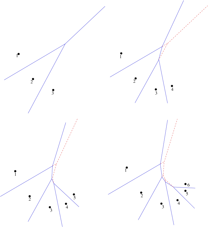
Figure 4.4: Worst-case Sequence of Additions to a Voronoi Diagram

A lower bound for the performance of any dynamic algorithm is the amount of structure update in the output per addition or deletion. In 1-D, the structural change is the merging or splitting of one interval, which is $O(1)$. 1-D intervals extend to convex polytopic partitions in 2-D. We show (Lemma 4.1) that for 2-D Voronoi (and thereby, power) diagrams this lower bound is the number of existing partitions - i.e. $\Omega(n)$.

Lemma 4.1.

There exists a sequence of addition of points in an online construction of a Voronoi Diagram such that the amortized cost per addition is $\Omega(n)$.

Proof.

See Figure 4.4. ∎

Figure 4.4 shows points being added from left to right to a Voronoi diagram; each point is inside the circumcircle of the three points succeeding it. Each addition affects all existing regions in the partition. This sequence of points demonstrates that there are sequences of 2-D inputs for which the structure change for each update is $\Omega(n)$. In contrast, the cost of structure update in 1-D ($O(1)$) is independent of the sequence in which points are added.

If the input sequence is random, however, the expected structure update cost for every addition is $O(1)$ (see [8]). The algorithm randomizes choices made in maintaining an internal data structure. We report the efficiency of our algorithm as a sum of two components - deterministic and expected. The expected cost of locating one region affected by the update is $O(\log{n})$. This cost is independent of the input sequence. It is an expectation over random choices for the data structure. The other component is the deterministic cost of the structure change. If $k$ is this number of disks whose power regions are affected by a particular update then our algorithm updates the power regions, and corresponding coverage regions in $O(k)$.

4.3.2 Mapping between 2-D Power Diagrams and 3-D Convex Polytopes

An upper convex polytope in 3-D is the intersection of a set of 3-D half-spaces containing the point $(0,0,\infty)$. The method we propose for dynamic updates to power diagrams uses a mapping from 2-D disks to 3-D upper convex polytopes.

Consider a set of disks $\{C_{1},C_{2},\ldots,C_{n}\}$ in the $xy$-plane. Let $r_{i}$ be the radius, and $(x_{i},y_{i})$ be the center of disk $C_{i}$. Disk $C_{i}$ is mapped to the half-space $S_{i}\equiv z\geq 2xx_{i}+2yy_{i}-x^{2}_{i}-y^{2}_{i}+r^{2}_{i}$. The intersection of half-space $S_{i}$ with the paraboloid $z=x^{2}+y^{2}$ projects down to $C_{i}$.

This map is illustrated in Figure 4.5. The intersection of two disks, and their mapping to two intersecting 3-D half-spaces is shown in Figure 4.6.

Figure 4.5: Mapping a Disk to a Half-Space (courtesy [6])

Figure 4.6: Two Intersecting Disks Map to Intersecting Half-Spaces (courtesy [31])

The upper convex polytope formed by the intersection of the half-spaces $\{S_{1},S_{2},$ $\ldots,S_{n}\}$ is dual to the power diagram of the disks $\{C_{1},C_{2},\ldots,C_{n}\}$. This claim is proved in [5].

Figure 3.10 shows a power diagram containing disks with empty power regions. The mapping described here leads to a characterization of such disks - in terms of half-spaces we call redundant. A half-space $S$ is redundant if the convex polytope formed by $\{S_{1},S_{2},\ldots,S_{n}\}$ is not changed by the addition of $S$. The mapping described here implies a duality between redundant half-spaces and disks with empty power regions.

Dynamic maintenance of the 2-D power diagram during addition or deletion of a disk corresponds to dynamic maintenance of the dual 3-D convex polytope during addition or deletion of the mapped half-space. The 2-D partition into power regions is obtained by projecting down from the 3-D convex polytope. This projection maps the 2-D faces of the 3-D convex polytope to power regions in 2-D.

In the remainder of this section we do not explicitly state our arguments in the context of 2-D power regions. Instead, we formulate our arguments in terms of faces of the corresponding convex polytope.

4.3.3 Dynamic Maintenance of a 3-D Convex Polytope

The best known dynamic 3-D convex polytope maintenance algorithm is by Chan [32]. However, this algorithm does not construct the new faces explicitly. We choose an approach described in Mulmuley [7, Chapter 4]). This algorithm constructs the new faces (i.e. 2-D partitions) which we require to compute disk intersections. Our approach, however, requires special treatment of redundant half-spaces; Chan’s algorithm does not. We discuss redundant half-spaces in more detail in Section 4.5.

Our approach for dynamic maintenance of a 3-D convex polytope follows that of Mulmuley [7, Chapters 3 and 4], which presents an algorithm for online construction of a convex polytope. We will refer to the analysis of this algorithm in the analysis of the dynamic algorithm. We do not, however, reproduce the online algorithm or its analysis in this report.

Facial Lattice of a Convex Polytope

The ‘facial lattice’ of a convex polytope is the adjacency relation between its vertices, edges, and faces. Each addition of a half-space causes a change to the facial lattice. Vertices, edges, and faces that do not belong to the half-space are removed. New vertices, edges, and faces are created corresponding to the intersection of the added half-space to the existing polytope. This operation may be viewed as splitting the faces of the polytope intersecting with the new half-space; the portion of the split polytope outside the half-space is removed, and a new face corresponding to the boundary of the intersection is created.

The size of the facial lattice of a convex polytope constructed with $i$ half-spaces is $O(i)$. $i$ half-spaces contribute to at most $i$ faces. Using this in Euler’s formula, we can show a bound of $O(i)$ on the number of edges and vertices as well.

Shuffle - A Randomized Data Structure

We adopt the terminology Shuffle from Mulmuley [7]. Each added half-space is assigned a random priority from the interval $(0,1)$. We begin the description of Shuffle by assuming that half-spaces are added in order of increasing priority. Later, we describe the operations of adding and deleting a half-space from an arbitrary position in the order. We denote Shuffle by $\mathbb{S}$.

We further assume that the bounded edges and faces of the polytopes we build are included in a large 3-D cube $\mathbb{C}$. This assumption serves only to simplify our description, and we later show how it may be removed.

$\mathbb{S}$ contains nodes for vertices and half-spaces, and represents a relation between these nodes. We will describe these nodes and relation shortly. $\mathbb{S}$ has eight root vertex nodes. These root nodes correspond to the vertices of $\mathbb{C}$.

When a half-space is added to a polytope, a new face and some new vertices are created. Some edges are split, and some edges are deleted. $\mathbb{S}$ records these actions as follows:

$vertex(v)$: vertex corresponding to the vertex node $v$

$created(v)$: half-space that creates vertex $v$

$next(u)$: for edge $\{u,v\},\ u\not\in S$ split at $w$, this the vertex $w$

$prev(w)$: for edge $\{u,v\},\ u\not\in S$ split at $w$, this the vertex $u$

$createdFace(S)$: list of vertices created by $S$, in order of face traversal

$deletedEdges(S)$: list of edges deleted by $S$, in order of traversal

The first half-space added, $S_{1}$, splits some faces of $\mathbb{C}$. The resultant polytope is $S_{1}\cap\mathbb{C}$. Vertex nodes corresponding to the new vertices are added to $\mathbb{S}$. The relation described by $created,\ next,\ prev,\ createdFace,$ and $deletedEdges$ is created.

This process is repeated for each addition. Consider the addition of (a non-redundant) half-space $S$ to polytope $H$. The resultant polytope is $S\cap H$. New nodes that correspond to the new face are created in $\mathbb{S}$. The relations $created$ and $createdFace$ are updated accordingly. The relations $next$ and $prev$ are updated to reflect the split of each edge. Edges deleted are added to the list $deletedEdges$.

Each vertex node corresponds to a vertex in some polytope $\supseteq H$. $prev$ is not defined for root nodes (corresponding to vertices of $\mathbb{C}$). A vertex node $v$ for which $next(v)$ is not defined is a leaf vertex node. Non-leaf vertex nodes correspond to polytopes constructed from half-spaces with priority less than $S$. We use $next$ and $prev$ to traverse from root to leaf, as described below.

Half-Space Intersection using Shuffle

In order to compute the intersection of a half-space $S$ with a polytope $H$, we first locate one intersection point, and then the rest of the intersecting face by traversal on other faces of $H$. We first show the use of $\mathbb{S}$ to locate an intersection point.

Algorithm 4.2 (TraverseShuffle(S)).

1. Find a root node $u$ such that $vertex(u)\in\mathbb{C}\setminus S$

2. $v\leftarrow next(u)$

3. if $v=\phi$ return $u$ // reached vertex $u$ of $H$

4. Find a vertex $w$ on $createdFace(created(v))$ such that $w\not\in S$

5. if such a $w$ exists, then $u\leftarrow w$; repeat 2

6. if no such $w$ exists, then return $\phi$ // $S$ is a redundant half-space

We use the routine TraverseShuffle to locate a vertex $v\in H\setminus S$. Since $H\setminus S$ is a connected convex polytope, we can traverse all faces either intersecting $S$ or outside $S$ starting from the adjacencies of $v$. We construct the new polytope on this second traversal. If we find a face that is outside $S$, we remove it from the facial lattice. If we find a face that intersects $S$, we traverse that face on the path defined by the vertex adjacencies. During this traversal, we remove edges that lie outside $S$, and split edges that intersect $S$. A new edge is added between the two new vertices on this face. After traversing one face, we move to a face with a common edge that is either outside $S$ or intersects $S$. Doubly-Connected Edge List - a data structure for maintaining the facial lattice efficiently is described in the book by de Berg et al. [33].

Analysis - TraverseShuffle and Intersection

We first prove the correctness of TraverseShuffle; that is it returns $\phi$ if and only if $S$ is redundant for $H$.

Lemma 4.2.

TraverseShuffle returns $\phi$ if and only if $H\subset S$

Proof.

If $x\not=\phi$ is returned, then the path followed by the algorithm ensures that $x\in H\setminus S$, thus $H\not\subset S$.

Suppose $\phi$ is returned. Let $u$ be the last vertex node visited; and $H_{u}$ be the corresponding polytope when $u$ was created. Let $v=next(u)$; and $H_{v}$ be its corresponding polytope. We can imagine the traversal from $u$ to $v$ as a traversal from the outer surface of $H_{u}$ to the outer surface of $H_{v}$. Since no vertex on the face creating $v$ is outside $S$, no point in $H_{v}$ is outside $S$ either. Since $H_{v}\supset H$, $H\subset S$.

Thus, $\phi$ is returned if an only if $H\subset S$. ∎

We use the online algorithm for polytope construction in [7]. This algorithm is analyzed probabilistically, assuming that the input sequence of half-spaces was drawn from a uniform random distribution. So far in this presentation we have assumed that additions are made in increasing order of priority. Thus, this model and assumption are the equivalent to the online algorithm from [7].

The data structure from [7] - history - is built on the same principles as $\mathbb{S}$. Thus, the analysis of TraverseShuffle is the same as that of search in history. TraverseShuffle thus performs in expected $O(\log{n})$ time.

The method of half-space intersection is also carried over from [7]. We have only used a random sequence as a conceptual tool to aid the analysis so far; whereas the algorithm input may be an arbitrary sequence. Hence, the cost of an addition is deterministic. If $k$ faces intersect with $S$, $O(k)$ is the size of the facial lattice of $S\cap H$. Thus, the addition of $S$ costs $O(k)$.

We now show the addition of a half-space $S$ with a random priority $p$. Unlike the assumption so far, this priority is not necessarily higher than all existing priorities.

Our approach is similar to Section 4.2. We first add the half-space to the end of the sequence, and then move it up the sequence using rotations in $\mathbb{S}$. We will see that these rotations are analogous to the rotations described for the treap in Section 4.2.

Note that the output polytope is independent of the sequence of additions; our purpose of rotations is only to manipulate the data structure. This manipulation is required to maintain the $O(\log{n})$ expected search guarantee shown earlier. The purpose of the rotation is to maintain the data structure such that it appears as if all half-spaces were added in increasing priority order.

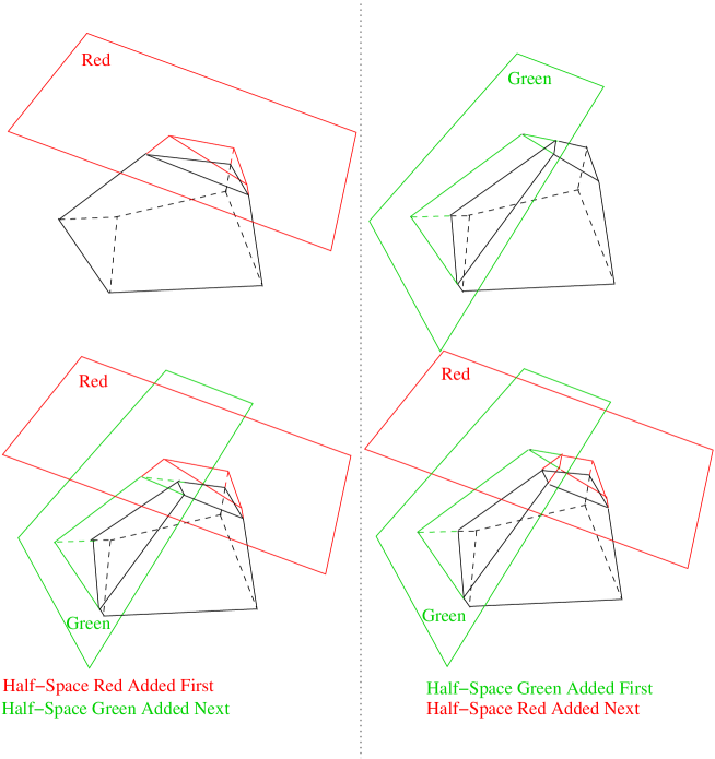
Figure 4.7: Addition of Half-Space to Polytope

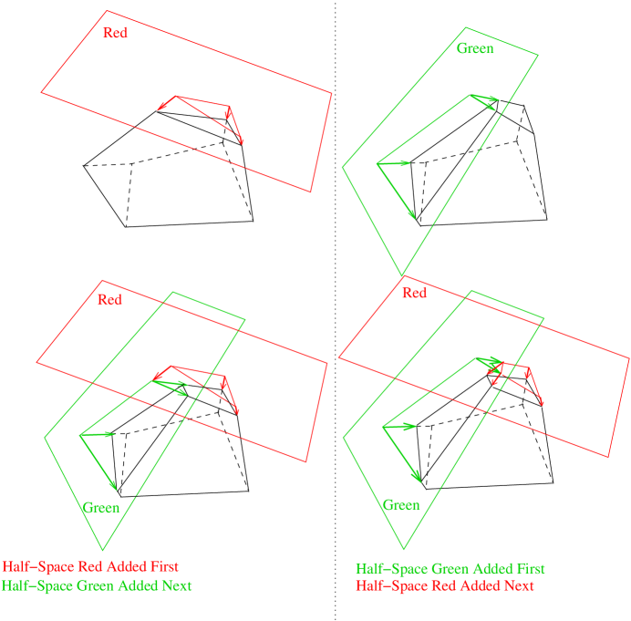
Figure 4.8: Data Structure changes for Addition

Algorithm 4.3 (Rotate-Addition).

1. $L\leftarrow\phi$ // $L$, set of half-spaces

2. for each $v\in createdFace(S)$, do

   1. $S^{\prime}\leftarrow created(prev(v))$

   2. add $S^{\prime}$ to $L$

3. for the highest priority half-space $S^{\prime}\in L$, do

   1. $S^{\prime}\leftarrow$ highest priority half-space in $L$

   2. traverse $createdFace(S^{\prime})$ and $deletedEdges(S^{\prime})$ to build polytope $\mathbb{A}=S^{\prime}\setminus H$

   3. traverse $\mathbb{A}$ to build polytope $\mathbb{A^{\prime}}\leftarrow\mathbb{A}\setminus S$

   4. use $\mathbb{A^{\prime}}$ to update relations for $S$ and $S^{\prime}$ // switch order of intersection

   5. $L\leftarrow L\setminus\{S^{\prime}\}$

Figure 4.7 shows the addition of two distinct half-spaces to a 3-D polytope. Since set intersection is commutative, the order of addition does not change the resultant polytope. However, the facial lattice changes are distinct. Figure 4.8 shows the two different search structures arising from the two sequences.

This algorithm is adapted from Mulmuley [7, Chapter 4]. Our algorithm is meant for use only with non-redundant half-spaces. It is the 2-D extension of treap rotation in Section 4.2. The operations Algorithm 4.3 performs on the facial lattice for addition of half-space Green, which has a higher-priority than half-space Red, is depicted in Figure 4.8. The relevant edges in the facial lattice are marked with arrow-tips. The sequence on the left shows the facial lattice before Step 3, and the sequence on the right shows the changes to the facial lattice after Step 3. The cost of each iteration of Step 3 is $O(|A^{\prime}|)$. The sum over all iterations is $O(k)$, where $k$ is the structure change due to addition of $S$.

Deleting a Half-Space

Deletion of a half-space $S$ from $H$ first requires a search for the corresponding face on $H$, and then updates for the part of the facial lattice that changes. The delete operation is the reverse of addition.

We first locate the corresponding face using $\mathbb{S}$. The traversal technique is the same as TraverseShuffle. Then we increase the priority of $S$ beyond that of its neighbors. This makes all vertices of $createdFace(S)$ leaves.

The update to $H$ is then removal of the face for $S$, and extension of neighboring faces using $deletedEdges(S)$ and $prev(v)$ for each vertex $v$ on $createdFace(S)$. Note that during addition, this update is performed in reverse - the new half-space is added as the highest priority order and moved up the priority order to fit its final position. Rotations are required here too to increase the priority for $S$. These too, are the reverse of rotations for addition.

Choice of Method

The choice of this particular method of random priorities with rotation is primarily motivated by the ready availability of the power frame during addition and deletion. We show this property in the next section and use this for disk intersections.

4.3.4 Open Problems

Analyses for addition and deletion are given in Mulmuley [7] that shows $O(\log{n})$ expected time. However, the analysis requires assumption of a random sequence. The cost of rotations in a random sequence is $O(1)$. Additionally, this result is derived as a corollary of results on configuration spaces. We conjecture that this analysis can be simplified to $O(\log{n})$ expected search and rotation time under our assumption of non-redundant half-spaces.

We assumed a bounding cube at the beginning of this section. Removing this assumption is possible by assigning non-numerical symbolic values to vertices on $\mathbb{C}$ and its split edges.

4.4 Dynamic Disk Intersections

Updating a coverage map for adding a transmitter requires two sets of operations. The first set of operations compute the coverage region for the new transmitter. The second set of operations compute changes in the coverage regions of the new transmitter’s neighbors in the power diagram. We show dynamic methods for both sets of operations. Similar operations are required to delete a transmitter.

Algorithm 3.1 uses the power frame for a transmitter to compute its coverage region. The power frame helps us limit the number of arc intersections for each interfering neighbor. Two arc intersections are required per neighbor. For the same reason, we use the power frame for dynamic disk intersection as well.

4.4.1 Computing the power frame

Our method computes the power frame of an added or deleted transmitter in linear time. The addition of a half-space $S$ begins at the end of the priority order. Later rotations fix the data structure $\mathbb{S}$ to reflect the correct priority of $S$. We use this initial addition, before rotation, to get the power frame. Similarly, the last stage of deletion is used to get the power frame of the transmitter to delete.

In Algorithm 3.1, we compute the power diagram of neighboring disks to obtain a transmitter’s power frame. This computation takes $O(k\log{k})$ time for $k$ neighbors. In $O(k)$ time, however, we can traverse $createdFace(S)$, $prev(v)$ for each vertex $v$ on $createdFace(S)$, and $killedEdges(S)$. This traversal gives the power frame, just like the traversal to obtain $\mathbb{A}$ in Algorithm 4.3.

4.4.2 Using the Power Frame

The coverage region for a transmitter is represented by arc polygons (see Figures 3.4, 3.5, and 3.6). The coverage region for the added transmitter is computed exactly as in Step 4c of Algorithm 3.1. An interference arc corresponding to a neighbor is removed from each power partition, and the transmission arc is added.

The coverage region for neighboring transmitters must be updated to remove arcs corresponding to the new transmitter. Consider the addition of a new transmitter $\tilde{p}$, and a power neighbor $\tilde{q}$. We only have the power frame for $\tilde{p}$, and not $\tilde{q}$. Thus, the method in Algorithm 3.1 cannot be used.

We use the power frame of $\tilde{p}$ for this update. We also use additional information in the power diagram. Each edge of the power diagram corresponds to two neighbors. With each edge we maintain one pointer to the interference arcs (if any) for the two neighbors, and one pointer to their transmission arcs. Thus, given the edges of power frame for the new transmitter, we can lookup the interference arcs of old neighbors that need to be removed. Only the arcs that must be removed are then traversed in sequence in the coverage region. This method takes $O(k)$ time for updating $k$ neighboring coverage regions.

Deleting a transmitter requires only the update of its neighboring coverage regions, since removal of the deleted transmitter is trivial. Here too, we use the pointers to the transmission and interference disks, as outlined in the addition procedure. Each neighbor’s interference arc is added, and the deleted transmitter’s transmission and interference arcs are removed in sequence. This operation is $O(k)$ in general, the only special condition being when degenerate arcs (i.e. with one point) result. This condition can be avoided by the “standard assumption” that after any (addition or deletion) operation the underlying polytope does not contain a subset of four half-spaces intersecting in one vertex.

4.5 Hidden Disks and Redundant Half-Spaces

We call disks with empty power regions hidden disks. As remarked in Subsection 4.3.2, these disks are dual to redundant half-spaces in the 3-D upper convex polytope. Claim 3.1 implies that any coverage point must have a corresponding power region. Thus, disks with empty power regions contribute only to interference in the coverage map, and do not contribute to coverage.

3-D convex polytope construction is dual to 3-D convex hull construction. In this duality, points inside the convex hull map to redundant half-spaces. The mapping we use implies that hidden disks (in 2-D) map to points inside the 3-D convex hull. Thus, in a random deployment of disks, it is highly probable that a disk will be hidden (i.e. that the mapped 3-D point will lie inside the 3-D convex hull). However, in an arbitrary or planned deployment by software or a network designer, we don’t expect many redundant disks, since these do not contribute positively to coverage.

The efficiency of maintaining a dynamic 3-D convex hull depends on structure, as shown by the mapping from our lower bound in Section 4.3. However, even the problem of maintaining a location structure for $O(\log{n})$ query to decide whether a given point lies in the convex hull is open (see Demaine et al. [34]). The best known algorithm, by Chan [32], is polylogarithmic.

Our method gives $O(\log{n})$ performance simply because the deletion of any half-space does not ’expose’ a redundant half-space. Thus, we do not require to look through redundant half-spaces that have become non-redundant following a deletion. A data structure to maintain this lookup information is apparently hard to develop, hence the open problem.

We can, however, maintain a relation between hidden disks and power regions. Thus, during removal of a non-redundant disk, we lookup this relation to check whether the affected power regions contained a hidden disk that has now become ‘visible’. We claim that this method requires $kO(\log{n})$ time for update to a power region affecting $k$ redundant disks.

The union of all disks remains the same, regardless of the presence of hidden disks. We observe that dynamic maintenance of coverage without considering interference (sensor coverage, as in [3]) is still possible (by suitably modifying our methods) in $O(\log{n})$ time per update.

Chapter 5 Coverage in the SINR Model

In Chapters 3 and 4, we have shown algorithms in the protocol model that report and maintain the boundary of the wireless coverage map. This chapter shows that the partitioning model extends, by appropriate extensions to the distance measure, to the SINR model. We also show that the boundary of the coverage cannot neither be computed efficiently nor represented efficiently in a data structure. In this sense, this chapter is exploratory and lays a foundation for Chapter 6.

The SINR (Signal-to-Interference-plus-Noise-Ratio) model includes the effects of path-loss and aggregated interference from all transmitters into the coverage decision. Formally, the SINR model is defined as follows:
$T$: a set of transmitters
$P_{\tilde{t}}>0$: Transmit power of transmitter $\tilde{t}\in T$
$N_{0}>0$: Ambient noise power
$d(x,\tilde{t})$: Distance of point $x$ from transmitter $\tilde{t}$
$\alpha\geq 2$: Path-loss exponent
$SINR(x,\tilde{t})=\frac{\displaystyle\frac{P_{\tilde{t}}}{d(x,\tilde{t})^{\alpha}}}{\displaystyle\sum_{\tilde{u}\in T\setminus\tilde{t}}\frac{P_{\tilde{u}}}{d(x,\tilde{u})^{\alpha}}+N_{0}}$
$\beta>0$: Receive sensitivity
Point $x$ is said to be in coverage if $\exists\tilde{t}\in T$ such that $SINR(x,\tilde{t})>\beta$.

In this work, we study coverage in SINR for the following model parameters:

• Fixed 2-D transmitter locations

• Fixed values for $\alpha$, $\beta$, $N_{0}$, and $P_{\tilde{t}}\ \forall\tilde{t}\in T$

As in the case of coverage in the protocol model, we begin our analysis for the special case of all transmit powers being equal. The method developed for equal transmit powers is then generalized to unequal transmit powers. We also aim to generalize the methods to include statistical variations in the received signal energy - such as fading and shadowing.

A capture transmitter for any point $x$ in the plane is a transmitter $\tilde{t}$ for which $SINR(x,\tilde{t})\geq SINR(x,\tilde{u})\ \forall\tilde{u}\in T\setminus\tilde{t}$. The subset of points covered by a transmitter $\tilde{t}$ is the set of points captured by $\tilde{t}$ at which $SINR(x,\tilde{t})>\beta$.

Since we are interested in studying the coverage region for each transmitter, we first analyze the partition of the plane into the capture regions of the transmitters. The coverage regions are subsets of the capture regions.

5.1 Equal Transmit Powers: Voronoi Partitions and Capture Transmitters

The following lemma shows that the partition of the plane into capture regions is the Voronoi diagram of the transmitter locations. First we note that:

$$\frac{A}{M-A}\geq\frac{B}{M-B}\Leftrightarrow A\geq B,\ \forall A,B>0,\ M>A+B$$ (5.1)

Lemma 5.1.

If all transmit powers are equal, then a point $x$ is in the capture region of $\tilde{t}$ if and only if $x$ is in the Voronoi partition corresponding to $\tilde{t}$.

Proof.

$$SINR(x,\tilde{t})=\frac{\frac{P}{d(x,\tilde{t})^{\alpha}}}{\displaystyle\sum_{\tilde{u}\in T\setminus\tilde{t}}\frac{P}{d(x,\tilde{u})^{\alpha}}+N_{0}}$$

$$\Leftrightarrow SINR(x,\tilde{t})=\frac{\frac{P}{d(x,\tilde{t})^{\alpha}}}{\displaystyle\sum_{\tilde{u}\in T}\frac{P}{d(x,\tilde{u})^{\alpha}}+N_{0}-\frac{P}{d(x,\tilde{t})^{\alpha}}}$$

Let

$$A=\frac{P}{d(x,\tilde{t})^{\alpha}},\ \textrm{and}\ M=\sum_{\tilde{u}\in T}\frac{P}{d(x,\tilde{u})^{\alpha}}+N_{0}$$

Let $s$ be another transmitter in $T$, and $\displaystyle B=\frac{P}{d(x,\tilde{s})^{\alpha}}$

$$SINR(x,\tilde{t})\geq SINR(x,\tilde{s})\Leftrightarrow\frac{A}{M-A}\geq\frac{B}{M-B}\Leftrightarrow A\geq B$$

$$\Leftrightarrow\frac{P}{d(x,\tilde{t})^{\alpha}}\geq\frac{P}{d(x,\tilde{s})^{\alpha}}$$

$$\Leftrightarrow d(x,\tilde{t})\leq d(x,\tilde{s})$$

Thus, if $\forall\tilde{s},\ SINR(x,\tilde{t})\geq SINR(x,\tilde{s})$, then $\forall\tilde{s},\ d(x,\tilde{t})\leq d(x,\tilde{s})\Leftrightarrow x\in$ Voronoi partition of $\tilde{t}$. ∎

This lemma shows that the capture region for each transmitter lies in its Voronoi partition. This is similar to Claim 3.1 - for the protocol model for equal transmitter powers - which states that the coverage region of a transmitter lies inside its Voronoi partition.

In order to find the coverage region of a transmitter, we need to find the transmitter’s Voronoi partition, and then the set of points in this partition at which the SINR is at least $\beta$. Some examples of coverage region contours for varying $\beta$ are shown in Figures 5.1, 5.2, and 5.3.

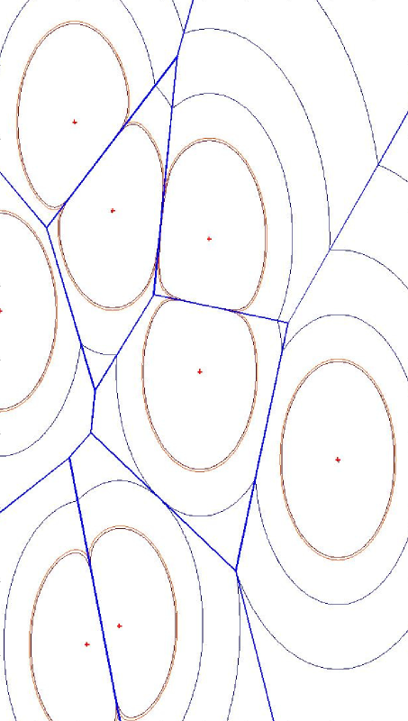
Figure 5.1: SINR Coverage: 8 Transmitters

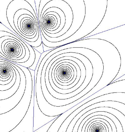
Figure 5.2: SINR Coverage: 6 Transmitters

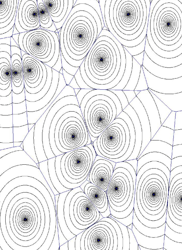
Figure 5.3: SINR Coverage: 25 Transmitters

We cannot represent the coverage region as a set of circular arcs, like the conic polygons in Chapter 3. Instead, we aim to approximate the boundary by a finite sequence of low-degree polynomial arcs. The choice of approximate boundary is such that the error in approximating the coverage region is bounded, and the number of evaluations of the SINR function required to build the representation is minimized.

Alt et al. [35] demonstrate an efficient strategy for approximate representation for convex areas. This may be extended to SINR coverage regions, if they can be shown to be convex. As we see later in Section 5.5, though, coverage regions are not convex in general. Some recent research has focussed on restrictions on the SINR model parameters that yield convex regions.

5.2 Concurrent Research in SINR Coverage

Research on similar lines has recently been reported by Avin et al. [10]: an approximation algorithm to decide whether a point $x$ is in a SINR coverage region. Our work was independently conceived. The algorithm in [10] is based on the following ideas:

1. Lemma 5.1,

2. The SINR coverage region $SINR(x,\tilde{t})>\beta$ is convex for $\alpha=2$ and $\beta>1$,

3. An error bound $\epsilon$, and approximate representation of the region $SINR(x,\tilde{t})>\beta$, and

4. An algorithm that uses this representation to decide coverage at a point within the error bound $\epsilon$.

Our work has more general aims:

1. We aim for an approximate representation for $\alpha\geq 2$, since $2\leq\alpha\leq 6$ for practical wireless environments (see [36]). This representation should also be valid for any $\beta>0$. The Voronoi partition contains points at which SINR $<1$, for which decoding is possible in practice.

2. We conjecture that the region $\{x|SINR(x,\tilde{t})>\beta\}\cap\triangle(\tilde{t})$ is convex. (Following the terminology from Table 3.1, $\triangle(\tilde{t})$ is the Voronoi partition corresponding to transmitter $\tilde{t}$) Thus, convexity is independent of $\beta$, but instead applies to the set of all points inside the capture transmitter’s Voronoi partition having SINR $>\beta$.

5.3 Convexity of SINR Coverage Regions in 2-D

We briefly review the definition of convexity, and outline our approach to proving convexity of the SINR coverage region.

Definition 5.1.

A set of points $S$ is a convex set if $\forall a,b\in S$, the set of all points $ka+(1-k)b,0<k<1$ is in $S$. In other words, if the end-points of any line segment $l$ lie in a convex set, then so does $l$.

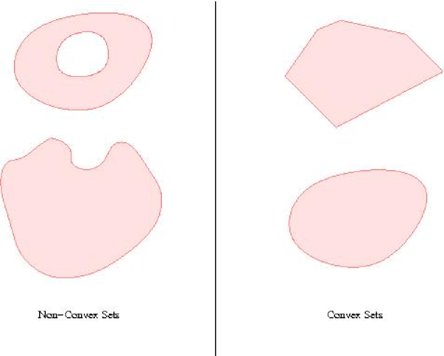
Figure 5.4: Examples of Convex Sets in 2-D

Figure 5.4 shows 2-D examples of convex and non-convex sets.

Applying this definition to the SINR coverage region:
Let $l_{p,q}$ denote the line segment between points $p$ and $q$. The SINR coverage region is convex if for all points $p$ and $q$ such that $SINR(p,\tilde{t})>\beta$ and $SINR(q,\tilde{t})>\beta$, the following is true: $SINR(x,\tilde{t})>\beta,\forall x\in l_{p,q}$.

Figures 5.1, 5.2, and 5.3 show convex SINR coverage regions for varying values of $\beta$. Many other experiments we conducted also suggest convexity.

A direct analytic proof of convexity would require calculating partial derivatives of the SINR formula. The intermediate expressions in such a proof would be hard to analyze due to the presence of the power $\alpha$, $2n$ constants corresponding to the transmitter locations in 2-D, and $N_{0}$.

Avin et al. [10] prove convexity for $\alpha=2$. This allows the SINR formula to be expressed as a polynomial of degree $2$ with $2n+1$ coefficients. Proving convexity is still a significant challenge, even with this simplification, as noted by the authors in the paper.

5.4 Convexity for $\alpha\geq 2$ and $\beta>0$

We now describe our approach to proving convexity of the SINR coverage region. We aim for a proof for $\alpha\geq 2$ and $\beta>0$. We have proved a restricted form of convexity called star-convexity for these parameters. In contrast, Avin et al. prove star-convexity also for $\alpha=2$. We conjecture that ideas in our proof for star-convexity can be generalized to prove convexity.

Definition 5.2 (Star-Convex Set).

A set $S$ is star-convex if $\exists r\in S$ such that for every line segment $l$ with $r$ as one end-point, and any other point in $S$ as the other end-point, all points in $l$ belong to $S$.

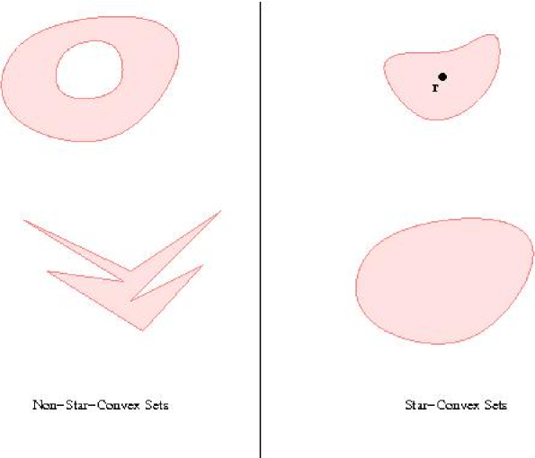
Figure 5.5: Examples of Star-Convexity in 2-D

2-D examples star-convex and non-star-convex sets are shown in Figure 5.5. All convex sets, by definition, are star-convex.

Some basic ideas in our approach follow:

1. Without loss of generality, we assume that $P_{\tilde{t}}=1,\ \forall\tilde{t}\in T$. The SINR function can be re-written as:

   $$SINR(p,\tilde{t})=\frac{1}{\displaystyle\sum_{\tilde{u}\in T\setminus\tilde{t}}\frac{d(p,\tilde{t})^{\alpha}}{d(p,\tilde{u})^{\alpha}}+N_{0}d(p,\tilde{t})^{\alpha}}$$

2. Since $SINR(p,\tilde{t})\geq\beta\Leftrightarrow\displaystyle\frac{1}{SINR(p,\tilde{t})}\leq\frac{1}{\beta},\ \forall\beta>0$, testing SINR coverage region convexity is equivalent to testing convexity for the region

   $$\sum_{\tilde{u}\in T\setminus\tilde{t}}\frac{d(p,\tilde{t})^{\alpha}}{d(p,\tilde{u})^{\alpha}}+N_{0}d(p,\tilde{t})^{\alpha}\leq\frac{1}{\beta}$$ (5.2)

3. We view the sum of terms in Inequality 5.2 as a function $f:\triangle(\tilde{t})\rightarrow R^{+}$. $f$ is a function of two variables. In order to prove convexity of the region $f\leq\frac{1}{\beta}$, we must analyze it on domains that are line segments $l_{p,q}$, for arbitrary points $p,\ q$ in the region $\triangle(\tilde{t})$.

   We denote the restriction of function $f$ to the domain $l_{p,q}$ by $f_{p,q}$. Since $l_{p,q}$ is a line segment, $f_{p,q}$ is a function of only one variable.

4. We use convexity terminology from Boyd et al. [37]. $f_{p,q}:l_{p,q}\rightarrow R$ is monotonic if: $f_{p,q}$ is differentiable and $\forall x\in l_{p,q},\ \frac{d}{dx}f_{p,q}$ has the same sign.

   $f_{p,q}$ is unimodal if $\exists x^{*}\in l_{p,q}$ such that $f_{p,x^{*}}$ and $f_{x^{*},q}$ are monotonic and $\frac{d}{dx}f_{p,q}(x)=0\Rightarrow\frac{d^{2}}{dx^{2}}f_{p,q}(x)\geq 0$.

   $f_{p,q}$ is quasi-convex if it is monotonic or unimodal. If $f_{p,q}$ is quasi-convex, then $\forall l_{p^{*},q^{*}}\subset l_{p,q},\ f_{p^{*},q^{*}}$ is quasi-convex.

   Lemma 5.2.

   In order to prove convexity of the region $f\leq\frac{1}{\beta}$, it suffices to prove that: for each pair of points $\{p,q\}$ on the boundary of the region, $f$ is quasi-convex on the line segment $l_{p,q}$.

5. We analyze each term in the sum separately, and then analyze the sum. The following lemma shows conditions for which monotonicity of individual terms extends to monotonicty of the sum:

   Lemma 5.3.

   If $f:R\rightarrow R$ and $g:R\rightarrow R$ are two functions monotonically increasing in an interval $[p,x^{*}]$ and monotonically decreasing in an interval $[x^{*},q]$, then the function $f+g$ is also monotonically increasing in $[p,x^{*}]$ and monotonically decreasing in $[x^{*},q]$. In other words, the sum of quasi-convex functions with the same mode(s) and directions of monotonicity is also quasi-convex.

6. In the quasi-convexity analysis for each term, we work with the power $2$ instead of $\alpha$. The following lemma shows that this approach is sufficient to prove quasi-convexity for any $\alpha$.

   Lemma 5.4.

   Consider a differentiable function $f:R\rightarrow R^{+}$. If $f$ is quasi-convex in interval $[a,b]$, then for all $\alpha>0$, $f^{\alpha}$ also quasi-convex in $[a,b]$.

   Proof.

   Monotonicity can be verified by differentiating $f^{\alpha}$:
   $\displaystyle\frac{d}{dx}f(x)^{\alpha}=\alpha f(x)^{\alpha-1}\frac{d}{dx}f(x)$. Since $\alpha>0$ and $f>0$, $\displaystyle\frac{d}{dx}f(x)^{\alpha}$ and $\displaystyle\frac{d}{dx}f(x)$ have the same sign. Thus, monotonic increase in $f$ is equivalent to monotonic increase in $f^{\alpha}$. Similarly, monotonic decrease is also equivalent for both functions.

   Since $\displaystyle\frac{d^{2}}{dx^{2}}f(x)^{\alpha}=\alpha f(x)^{\alpha-1}\frac{d^{2}}{dx^{2}}f(x)$ at ${x|\frac{d}{dx}f(x)=0}$, $\displaystyle\frac{d}{dx}f(x)^{\alpha}=0\Rightarrow\displaystyle\frac{d^{2}}{dx^{2}}f(x)^{\alpha}\geq 0$.

   $f^{\alpha}$ is quasi-convex in $[a,b]$. ∎

7. We want to prove convexity for the SINR coverage region in the Voronoi partition corresponding to each transmitter. Accordingly, we require to establish quasi-convexity for functions evaluated on line segments inside the Voronoi partition.

   The sum in Inequality 5.2 has two types of terms: $\displaystyle\frac{d(p,\tilde{t})^{\alpha}}{d(p,\tilde{u})^{\alpha}}$ and $N_{0}d(p,\tilde{t})^{\alpha}$. It is sufficient to show quasi-convexity for $\displaystyle\frac{d(p,\tilde{t})^{2}}{d(p,\tilde{u})^{2}}$ and $N_{0}d(p,\tilde{t})^{2}$, as shown by Lemma 5.4.

   We show quasi-convexity for the term $\displaystyle\frac{d(p,\tilde{t})^{2}}{d(p,\tilde{u})^{2}}$ on intersections of lines with the half-space $\hbar(\tilde{t},\tilde{u})$. This restriction to the half-space is sufficient, since the intersection of the half-spaces $\displaystyle\bigcap_{\tilde{u}\in T\setminus\tilde{t}}\hbar(\tilde{t},\tilde{u})$ is the Voronoi partition corresponding to $\tilde{t}$.

8. One final trick helps us to further simplify the analysis - rotation and translation of axes. Rotation and translation of axes do not alter the results of the analysis, since the distance function is invariant of these operations. Given line $l$ on which we need to evaluate a term, we rotate axes such that $l$ becomes the new $x$-axis. For evaluating the term $\displaystyle\frac{d(p,\tilde{t})^{2}}{d(p,\tilde{u})^{2}}$, we translate the axes such that the positive $x$-axis corresponds to $l\cap\hbar(\tilde{t},\tilde{u})$. (If $l\cap\hbar(\tilde{t},\tilde{u})=\phi$, then no translation is done.) This operation is shown in Figure 5.6.

   

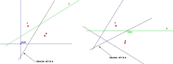
   Figure 5.6: Rotating & Translating Axes

   The following lemma shows quasi-convexity for the term $\displaystyle\frac{d(p,\tilde{t})^{2}}{d(p,\tilde{u})^{2}}$ evaluated on the $x$-axis. We choose, for this term, the brief notation $f_{t,u}$. We recall that $x>0$ corresponds to points on $l$ closer to $\tilde{t}$ than $\tilde{u}$ (see Figure 5.6). Figure 5.7 helps visualize the lemma.

   

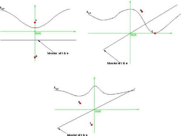
   Figure 5.7: $f_{t,u}\equiv\displaystyle\frac{d(p,\tilde{t})^{2}}{d(p,\tilde{u})^{2}}$ is quasi-convex for $x>0$

   Lemma 5.5.

   For an appropriate choice of $x$-axis, $f_{t,u}$ is quasi-convex on $x\geq 0$.

   Proof.

   Case 1:

   The bisector of $t$ and $u$ is parallel to $l$.

   Choose the line through $t$ and $u$ as the $y$-axis, and $l$ as the $x$-axis. Let $t\equiv(0,y_{t})$ and $u\equiv(0,y_{u})$ in this co-ordinate system.

   $f_{t,u}=\frac{x^{2}+y_{t}^{2}}{x^{2}+y_{u}^{2}}$. Since $t$ is closer to any point on $l$, $y_{t}^{2}\leq y_{u}^{2}$. Thus, $f_{t,u}$ is unimodal with minimum at $x=0$. This can be verified by differentiation:
   $\frac{d}{dx}f_{t,u}=\frac{2x(y_{u}^{2}-y_{t}^{2})}{(x^{2}+y_{u}^{2})^{2}}$.

   Case 2:

   The bisector of $t$ and $u$ intersects $l$.

   Choose $l$ as the $x$-axis, and the intersection point of $l$ with the bisector as the origin. Let $t\equiv(x_{t},y_{t})$ and $u\equiv(x_{u},y_{u})$ in this co-ordinate system.

   $f_{t,u}=\frac{(x-x_{t})^{2}+y_{t}^{2}}{(x-x_{u})^{2}+y_{u}^{2}}$. We verify unimodality of $f_{t,u}$ in $x\geq 0$ by differentiation:
   $\frac{d}{dx}f_{t,u}=\frac{2(x-x_{t})}{(x-x_{u})^{2}+y_{u}^{2}}-\frac{2(x-x_{u})}{((x-x_{t})^{2}+y_{t}^{2})^{2}}$
   Thus, the optima are at $x^{2}=x_{t}^{2}+y_{t}^{2}$. We can verify that $x=\sqrt{x_{t}^{2}+y_{t}^{2}}$ is a minima by substituting for $x$ in $f_{t,u}$.∎

9. Corollary 5.6 (Star-Convexity).

   The SINR coverage region is star-convex for $\alpha\geq 2$ and $\beta>0$.

   Proof.

   If one end-point of any line segment is always chosen to be the transmitter $\tilde{t}$, then minima of $f_{\tilde{t},u}$ for all $u$ are at $\tilde{t}$. Also, $d(x,\tilde{t})^{2}$ is convex on $x\geq 0$ with a unique minimum at $t$. Due to Lemma 5.4, the same monotonicity properties hold if we replace the power $2$ with the power $\alpha$. Since the minima coincide, the sum of quasi-convex terms are also quasi-convex, due to Lemma 5.3. ∎

10. A proof for convexity requires a generalization of Lemma 5.3 that excludes the pre-condition that all minima coincide. Though we see in Lemma 5.5 that all terms are unimodal, their minima occur at different points on the $x$-axis. We can show that the minima occur close together (within distance $|y_{t}|$ of each other), but a generalization of Lemma 5.3 eludes us.

5.5 SINR Coverage for Unequal Transmit Powers

Lemma 5.1 for equal transmit powers gives us a characterization of the SINR capture regions by Voronoi partitions - in terms of distance alone, i.e. independent of the transmit power(s). The partition of SINR capture regions for unequal transmit powers corresponds to “multiplicatively-weighted” Voronoi partitions. An example of a multiplicatively-weighted Voronoi diagram is Figure 5.8. The generalization of partitioning of SINR capture regions for unequal transmit powers is shown by the generalization of Lemma 5.1 below:

Lemma 5.7.

A point $x$ is in the capture region of transmitter $\tilde{t}$ if and only if $x$ is in the multiplicatively weighted Voronoi partition corresponding to $\tilde{t}$ with weight $P_{\tilde{t}}^{\frac{1}{\alpha}}$.

Proof.

$$SINR(x,\tilde{t})=\frac{\frac{P_{\tilde{t}}}{d(x,\tilde{t})^{\alpha}}}{\displaystyle\sum_{\tilde{u}\in T\setminus\tilde{t}}\frac{P_{\tilde{u}}}{d(x,\tilde{u})^{\alpha}}+N_{0}}$$

$$\Leftrightarrow SINR(x,\tilde{t})=\frac{\frac{P_{\tilde{t}}}{d(x,\tilde{t})^{\alpha}}}{\displaystyle\sum_{\tilde{u}\in T}\frac{P_{\tilde{t}}}{d(x,\tilde{u})^{\alpha}}+N_{0}-\frac{P_{\tilde{t}}}{d(x,\tilde{t})^{\alpha}}}$$

Let

$$A=\frac{P_{\tilde{t}}}{d(x,\tilde{t})^{\alpha}},\ \textrm{and}\ M=\sum_{\tilde{u}\in T}\frac{P_{\tilde{u}}}{d(x,\tilde{u})^{\alpha}}+N_{0}$$

Let $s$ be another transmitter in $T$, and $B=\frac{P_{\tilde{s}}}{d(x,\tilde{s})^{\alpha}}$

$$SINR(x,\tilde{t})\geq SINR(x,\tilde{s})\Leftrightarrow\frac{A}{M-A}\geq\frac{B}{M-B}\Leftrightarrow A\geq B$$

$$\Leftrightarrow\frac{P_{\tilde{t}}}{d(x,\tilde{t})^{\alpha}}\geq\frac{P_{\tilde{s}}}{d(x,\tilde{s})^{\alpha}}$$

$$\Leftrightarrow P_{\tilde{t}}^{\frac{1}{\alpha}}d(x,\tilde{t})\leq P_{\tilde{s}}^{\frac{1}{\alpha}}d(x,\tilde{s})$$

Thus, if $\forall\tilde{s},\ SINR(x,\tilde{t})\geq SINR(x,\tilde{s})$, then $\forall\tilde{s},\ P_{\tilde{t}}^{\frac{1}{\alpha}}d(x,\tilde{t})\leq P_{\tilde{s}}^{\frac{1}{\alpha}}d(x,\tilde{s})\Leftrightarrow x\in$ multiplicatively-weighted Voronoi partition of $\tilde{t}$. ∎

The generalization to unequal powers is similar to the generalization of Voronoi diagrams to Power diagrams introduced in Chapter 3. In fact, another term for the Power Diagram is “additively-weighted” Voronoi diagram (see [6]).

As seen in Figure 5.8, the multiplicatively-weighted Voronoi partition is not convex. Hence, we must relax the constraint of representing the SINR region by approximating a convex region.

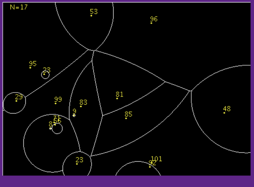
Figure 5.8: Multiplicatively Weighted Voronoi Diagram (courtesy [38]

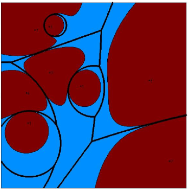
Figure 5.9: Non-Star-Convex Coverage Region

Furthermore, as seen in Figure 5.9, the coverage region for a transmitter may not be star-convex if all transmitters do not have the same power. Thus, it is hard to follow a geometric algorithm approach to coverage area computation for the SINR model.

Chapter 6 Coverage Optimization

In this chapter we propose an algorithm that optimizes coverage by choosing an apt transmit power assignment to transmitters operating on the same channel. Though it is desirable to solve this problem exactly in an analytical framework, it is observed that this would require solutions to implicit non-linear equations in many variables (see Section 6.3). Thus, to solve this optimization problem, we propose a derivative-free approach with the Random Hill Climbing algorithm. We demonstrate the efficiency of this algorithm using the SINR model. An important advantage of this algorithm is that it uses a coverage estimation procedure that can accommodate any deterministic coverage model.

In this chapter we presents simulation results to justify the performance of the proposed algorithm by comparison with optimization results using the Nelder-Mead method [39] and exhaustive search.

The rest of the chapter is organized as follows: The remainder of this section describes related work and notation. Section 6.3 initiates discussion and background for our solution approach. Section 6.4 describes methods we have analyzed for optimizing coverage, Section 6.5 presents an experimental comparison of these methods.

6.1 Related Work

Ahmed et al. [11] study optimum transmit power assignments to access points assuming a protocol model. Some optimization problems in link scheduling and power control in the SINR model are closely related to our problem. Goussevskaia et al. [15] show that a discrete problem of ‘single-shot scheduling’ with weighted links is NP-hard. Lotker et al. [16] and Zander et al. [17] give efficient algorithms for optimizing the maximum achievable SINR in a set of links. Yates et al. [18] report an algorithm to optimize the total uplink transmit power for users served by a base station, assuming that all users meet the minimum SINR constraint. A recent study by Altman et al. [19] considers SINR games played co-operatively and co-optively between base stations to maximize coverage area for mobile receivers or determine optimal placement for base stations themselves.

A more recent study of coverage optimization algorithms for indoor coverage appears in Reza et al. [20]. A new optimization model based on extrapolation of data collected from measurement tools is given by Kazakovtsev in [21].

In contrast to these studies, our work reports a method to obtain the power assignment that maximizes the coverage area; that is, the power assignment that enables the maximum possible number of receivers to meet the SINR constraint. Our Random Hill Climbing procedure is inspired by Mudumbai et al. [14]. They report a randomized procedure to synchronize multiple transmissions to send a common message coherently in a distributed beamforming system.

6.2 Notation

We use the following assumptions:

1. A receiver is in coverage if the SINR due to some transmitter is above a given threshold.

2. Transmitter locations are fixed; and all transmitters lie in the plane. We measure the coverage area within a bounding rectangle.

3. All receivers have the same receive sensitivity. All transmissions are omni-directional.

The notation we use is as follows:

1. $T$ denotes the set of transmitters. All transmitters lie in an axis-parallel rectangle $E$ of unit area.

2. The transmit power of transmitter $t\in T$ is denoted $P_{t}$. The transmit power is bounded, i.e., $P_{t_{min}}\leq P_{t}\leq P_{t_{max}},\forall t\in T$.

3. $\hat{P}$ is the $|T|$-dimensional vector of power assignments.

4. $d(x,t)$ denotes the Euclidean distance between a point $x$ and transmitter at $t$.

5. $\alpha$ is the path-loss exponent. In free space $\alpha=2$, and other values are experimentally or analytically derived from the propagation environment [36, Chapter 2].

6. The receive power $R(x,t)$ at point $x$ from transmitter $t$ is ${P_{t}}/({d(x,t)^{\alpha}})$.

7. $N_{0}$ is the the ambient noise power.

8. $SINR(x,t)$ denotes the SINR at point $x$ due to transmitter $t$.

   $$SINR(x,t)=\frac{R(x,t)}{\sum_{s\in T\setminus\{t\}}R(x,s)+N_{0}}$$ (6.1)

9. $\beta$ is the minimum SINR required for successful reception.

10. The maximum SINR at a point $x$, denoted $SINR_{max}(x)$, is the maximum of $SINR(x,t)$ over the set of transmitters $t\in T$.

11. The coverage area $\mathbb{C}$ is the measure of the area of the set $\{x|SINR_{max}(x)\geq\beta\}\cap E$. Note that $\mathbb{C}$ is a function of the transmitter locations and their power assignments.

It must be noted that all instances of $SINR(x,t)$ and $SINR_{max}(x)$, and $\mathbb{C}$ as well, are functions with domain as the universe of vectors $\{\hat{P}\}$.

6.3 Optimization Problem Solution Approach

We are interested in an optimization method that yields a global maximum for function $\mathbb{C}$. In this section we describe the characteristics of the objective function $\mathbb{C}$, and justify our choice of optimization method. Optimization methods for non-linear functions (such as $\mathbb{C}$) are broadly classified as gradient-based methods and direct-search methods [39]. In gradient-based methods, the gradient vector - comprising the first order partial derivatives of the objective function is required. Thus, the objective function must be continuous and differentiable over the feasible set. Further, its partial derivatives must be expressible in an analytical form (“closed-form expression”).

Optimization of objective functions that are non-differentiable or do not have closed-form expressions requires a heuristic method to iterate through feasible solutions efficiently. Such a method is called a direct search method.

Our objective function $\mathbb{C}$ has domain $\hat{P}$ - the vector of power assignments. $\mathbb{C}$ is the measure of the area of the region $\{x|SINR_{max}(x)\geq\beta\}\cap E$. However, the measure of this area is not expressible in analytical form; and thereby, the partial derivatives of $\mathbb{C}$ are not available in analytical form either.

We must choose a direct search method to maximize $\mathbb{C}$. Further, since $\mathbb{C}$ does not have an expression in analytical form, its values required in the execution of the maximization program must be estimated by numerical methods. The following section describes our methods for estimating the coverage area, and direct search methods for coverage area optimization.

6.4 Proposed Solution Method Details

6.4.1 Estimating the Coverage Area

The coverage area is estimated as follows: We choose an appropriate finite sample set of points in $E$, and report the estimate of $\mathbb{C}$ as the fraction of this sample for which $SINR_{max}\geq\beta$. (Note that $E$ is of unit area.) Computing this fraction involves computations of $SINR_{max}(x)$ for all sample point $x$. Each computation of $SINR_{max}$ is $O(|T|)$. We propose two methods for choosing the sample:

1. The set of points on an axis-parallel grid on $E$.

2. A random finite set of points in $E$.

The accuracy of the estimate depends on the size and distribution of the sample. However, we can obtain probabilistic guarantees on the number of samples required for a desired level of accuracy as follows.

Let the desired estimation error ratio be $\epsilon\in(0,1)$; that is, the estimated area lies in $\left[(1-\epsilon)\mathbb{C},(1+\epsilon)\mathbb{C}\right]$ with probability $\delta$.

We present a method to arrive at a ‘sufficient’ number of random samples or grid points for a desired accuracy ratio. Let $X\in\{0,1\}$ be an indicator random variable corresponding to the event of a sample point belonging in the coverage area. Thus, $Pr(X=0)=1-\mathbb{C}$ and $Pr(X=1)=E_{X}=\mathbb{C}$. Let $S_{n}$ be the random variable corresponding to the sum of $n$ sampling events. In context, $\frac{S_{n}}{n}$ is the estimated area.

By Chernoff’s bound [40], we know that:

$$n>\frac{3ln(\frac{2}{\delta})}{\epsilon^{2}\mathbb{C}}\Rightarrow Pr(|\frac{S_{n}}{n}-\mathbb{C}|\leq\epsilon\mathbb{C})\geq 1-\delta$$ (6.2)

Thus, we can choose $n$ by setting the estimation error $\epsilon$ and probability guarantee $\delta$ suitably.

The grid comprises of lines parallel to the axes. We could not find an analytical method for deriving the number of grid lines required for a desired estimation error. However, as a thumb rule, we use four times the number of points as in the random sample. Using the inequality in 6.2, for a desired accuracy of $85\%$ with an probability guarantee of $90\%$, we need to sample $400$ points. For these accuracy and guarantee parameters, we use $1600$ points in the grid.

In later sections, we refer as EstimateArea the subroutine that estimates the coverage area given the transmitter locations and power assignment. In order to give deterministic guarantees in comparisons of optimization algorithms, we use the grid method; otherwise, each run of an algorithm will use different sample points, and differences of accuracy between two algorithms may be due to the random choice of sample points.

We note that this estimation method can be extended to real world propagation models, such as espoused by project WINNER [41], by coding them as subroutines that compute receive powers at a sample point.

6.4.2 Direct search methods

A direct search maximization method iterates through choices of vectors in the feasible set without recourse to the gradient. We have analyzed two direct search methods - Random Hill Climbing and Nelder-Mead. We also include an exhaustive search method as a baseline for comparing the accuracy and power efficiency of these methods.

Exhaustive Search

The input to this algorithm is the set of transmitter locations and their power thresholds. The output of this algorithm is a power assignment to the transmitters that maximizes the coverage area. This algorithm discretizes the power assignment into levels, and returns the level vector that maximizes the coverage area.

This algorithm iterates through $k$ levels of power for each transmitter and executes the subroutine $EstimateArea$ $k^{|T|}$ times. The subroutine $nextVec$ returns the next power vector in some sequence. In our implementation, we have chosen this sequence in increasing order of total power, such that the added objective of finding the minimum total power that maximizes the coverage is also achieved. This algorithm serves as a benchmark to evaluate the accuracy and total power reported of the other methods we study: Random Hill Climb and Nelder-Mead.

Random Hill Climbing

This optimization procedure iteratively generates random vector increments to the current best known feasible solution. It then updates the best known solution with the incremented vector if the objective function value on the increment is better than the best known value.

We have implemented a variant of Random Hill Climbing for maximizing the coverage area.

We ran a large set of experiments with different parameters to compare this procedure with Exhaustive Search to evaluate convergence and maxima for a small set of transmitters. We also verified that, for large networks, it converges faster than another well-known deterministic procedure - Nelder-Mead. The details of these analyses follow later in Section 6.5.

This algorithm also uses the subroutine $EstimateArea$.

Algorithm 6.4 (RandomHillClimbing(T, $P_{min}$, $P_{max}$)).

  $\hat{bestP}\leftarrow P_{min}$

  $bestEstArea\leftarrow 0$

  repeat

     $attempts\leftarrow 0$

     $scaleUp\leftarrow 1+scaleFactor$

     $scaleDown\leftarrow 1+scaleFactor$

     $\hat{shrinkIncr}\leftarrow stepSize\cdot(P_{max}-P_{min})$

     $\hat{stretchIncr}\leftarrow stepSize\cdot(P_{max}-P_{min})$

     $localMaxima\leftarrow FALSE$

     while $(attempts<maxIterations)$ and $(localMaxima=FALSE)$ do

        $attempts\leftarrow attempts+1$

        if $attempts>scaleUpIncr$ then

           $scaleUp\leftarrow 1+2\cdot scaleFactor$

        end if

        if $isEvenNumber(attempts)$ then

           $\hat{shrinkIncr}\leftarrow\hat{shrinkIncr}/scaleDown$

           $\hat{t}\leftarrow\hat{bestP}+getRandom(0,\hat{shrinkIncr})$

        else

           $\hat{stretchIncr}\leftarrow\hat{stretchIncr}\cdot scaleUp$

           $\hat{t}\leftarrow\hat{bestP}+getRandom(0,\hat{stretchIncr})$

        end if

        Scale $\hat{t}$ to fit values in range specified by $P_{min}$ and $P_{max}$

        if $EstimateArea(T,\hat{t})>bestEstArea$ then

           $bestEstArea\leftarrow EstimateArea(T,\hat{t})$

           $\hat{bestP}\leftarrow\hat{t}$

           $localMaxima\leftarrow TRUE$

        end if

     end while

  until $attempts\geq maxIterations$

  return  $bestEstArea$, $\hat{bestP}$

Table 6.1 describes the parameters used in the Random Hill Climbing algorithm described in Algorithm 6.4. Each iteration of the inner loop checks whether a random increment to the best known vector ($\hat{bestP}$) gives a higher maximum. Random increments increase on odd numbered attempts and reduce on even numbered attempts. This bi-directional approach covers both steep and shallow saddle points: a large increment exits a shallow saddle point, whereas a small increment exits a steep saddle point. Further, to exit a wider shallow region, the rate of increment increases after $scaleUpIncr$ attempts.

When an improved best estimate of a local maxima is found, the outer (repeat) loop resets the increments. If no better estimate is found after $maxIterations$ of the inner loop, the procedure exits with the current estimate. Since the outer loop iterates through increasing estimates of local maxima, the returned result is an estimate of the global maxima.

Table 6.1: Random Hill Climbing Parameters

Parameter	Description	Simulation values
scaleFactor	Controls magnitude of the next random increment	$0.05\alpha$
stepSize	Controls initial magnitude of random increment	$0.01$
maxIterations	Maximum number of attempts to exit local maximum	2000
scaleUpIncr	Number of attempts after which random increment magnitude increases	100

Nelder-Mead

The Nelder-Mead is a well-known direct method for local optimization. Implementations are available in many public forums, and numerical packages like MATLAB have standard implementations. Even though it is an unconstrained optimization method, constraints can be handled by penalty functions [39].

We have adapted an implementation by Flanagan (available online at [42]). A detailed description of the algorithm is found in [39]. We use a random vector to initialize the method, and maintain the default parameter values of the algorithm.

We describe the Nelder-Mead method informally: It maintains a simplex of $n+1$ points (vertices). At each iteration, either a vertex is replaced or the simplex is shrunk. First, the vertex with the least image is chosen as origin, and three new vertices are generated in the direction of the median of the face formed by excluding this vertex. These new vertices are called vertex “contraction inside”, “contraction outside” or “expansion”. Of these three, the vertex the highest image is chosen as a potential new vertex. If this vertex has image higher than the origin (i.e. current least), then this vertex is replaces the origin. Otherwise, the simplex is “shrunk”, i.e. the face opposite the vertex with the highest image is scaled down. This replacement and shrink procedure continues until the difference between the least and highest image is below a convergence threshold.

The parameters of the Nelder-Mead algorithm are the distance of the three potential vertices from the origin, the shrink factor, and the convergence threshold. We have used the default values for these factors: $0.5$ for contraction and shrink, and $2$ for expansion.

The Nelder-Mead only returns a local maximum. In order to get the global maximum, we run the algorithm a number of times with random initial vectors.

Post-processing

We use a post-processing routine to try improve the coverage area by forcing smaller values to $P_{t_{min}}$. This routine iteratively sets the lowest $i\in\{1\ldots|T|\}$ powers to their corresponding values in $P_{min}$.

Another advantage of the post-processing routine is when the designer wants to find a subset of the input transmitters that is sufficient to attain maximum coverage. We can run an optimization procedure by setting $P_{min}$ to $\hat{0}$. Transmitters that have been assigned power $>0$ are sufficient, and those assigned power $0$ may be removed from the network.

The experiments we present in Section 6.5 use this post-processing on the output of Random Hill Climbing and Nelder-Mead.

Algorithm 6.5 ($postProcess(T,\hat{v},P_{min})$).

  $\hat{u}\leftarrow\hat{v}$ in increasing order

  $P_{0}\leftarrow P_{min}$ re-ordered to maintain the mapping with $\hat{v}$ in the sorted order

  $bestEstArea\leftarrow 0$

  $\hat{bestP}\leftarrow\hat{u}$

  for $i=1\to|T|$ do

     Set first $i$ values in $\hat{u}$ to first $i$ values in $P_{0}$

     if $EstimateArea(T,\hat{u})>bestEstArea$ then

        $bestEstArea\leftarrow EstimateArea(T,\hat{u})$

        $\hat{bestP}\leftarrow\hat{u}$

     end if

  end for

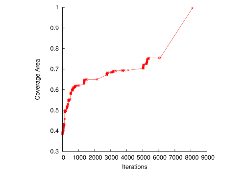
Figure 6.1: One simulation-based realization of Random Hill Climbing algorithm is illustrated in this figure.

Figure 6.1 shows the realization of the algorithm Random Hill Climbing followed by post-processing. This figure shows the estimates for the local maximum for the coverage area increasing by iterations of the inner loop. The final increment is due to the post-processing.

6.5 Algorithm Comparisons: Experiments and Results

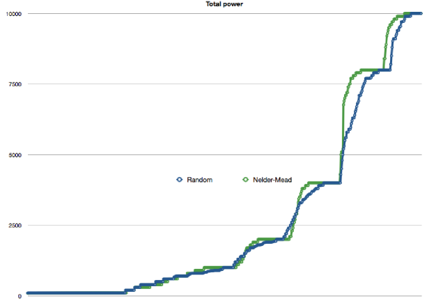
Figure 6.2: Comparisons of the total power used by each algorithm. The X-axis shows an internal variable for the experiment number. For better readability, the ordering of experiment numbers corresponds with increasing power.

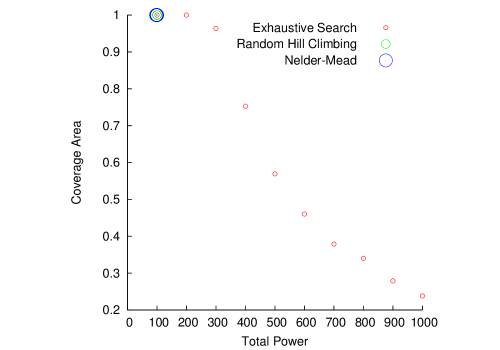
Figure 6.3: The tradeoff between coverage-area and total power is illustrated in this figure with $\alpha=2$, $N_{0}=10^{-5}$. The Random Hill Climbing and the Nelder Mead methods achieve the optimum-coverage transmit-power assignment.

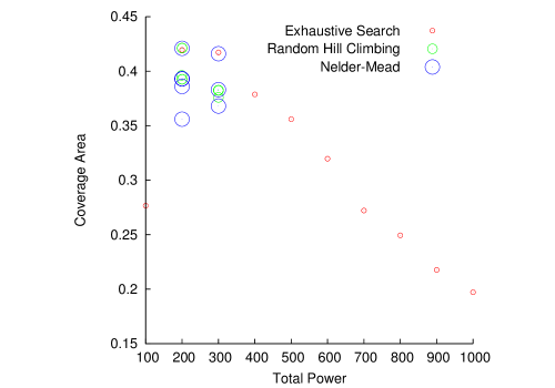
Figure 6.4: The tradeoff between coverage-area and total power is illustrated in this figure with $\alpha=2$, $N_{0}=10^{-3}$. The coverage-area increases initially from $0.28$ (noise-limited regime) towards $0.43$, and then it decreases (interference-limited regime). The Random Hill Climbing and the Nelder Mead methods achieve the optimum-coverage transmit-power assignment.

We have analyzed the coverage optimization algorithms with the following set of experiments. All experiments were run on a server with 8 quad-core processors and 8 GB of RAM. All algorithms were coded in Java, and run on a 64-bit server VM for J2SE 1.6.

Comparison with Exhaustive Search

We have compared the optimum obtained and total transmit power reported by the three algorithms for the following scenarios:

• Number of transmitters: 10

• $p_{min}=0$ and $p_{max}=100$ for all transmitters

• Values of $\alpha$: 2, 3

• Values of $N_{0}$: $10^{-3}$, $10^{-5}$

• Size of Grid: 40 X 40

All experiments are run with the same set of transmitter-locations. We show two of these results in Figures 6.3 and 6.4. We see that in both cases, both the total power consumed and coverage area reported by the Random Hill Climbing and the Nelder-Mead methods is comparable to the exhaustive search. The Nelder-Mead method may give a sub-optimal result, but since its execution time is small, it can be run multiple times and the best value can be chosen as the answer. Even with only $10$ transmitters, each run of Exhaustive Search takes about $11.5$ hours! Hence, we have restricted our comparison scenarios with Exhaustive Search to 10 transmitters.

Random Hill Climbing vs Nelder-Mead for 10 to 100 transmitters

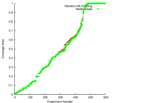
Figure 6.5: The optimum coverage-area ratio, as found by the Random Hill Climbing and the Nelder-Mead methods, is illustrated in this figure for up to 100 transmitters. The two methods are comparable in performance.

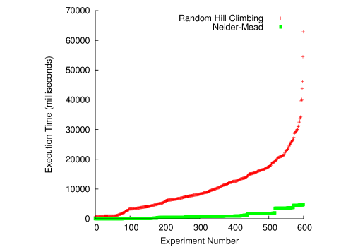
Figure 6.6: Execution time for Random Hill Climbing and Nelder-Mead for up to 100 transmitters is illustrated in this figure. Nelder-Mead runs faster.

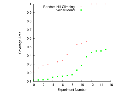
Figure 6.7: Optimum coverage-area found by Random Hill Climbing and Nelder-Mead for $\geq$ 500 transmitters is illustrated in this figure. Random Hill Climbing performs better.

Since these procedures run faster, we can run them with more transmitters. The following combinations were run, yielding a total of $600$ experiments:

• Number of transmitters: 10, 20, 40, 80, 100

• $p_{min}=0$ and $p_{max}=100$ for all transmitters

• Values of $\alpha$: 2, 3, 4

• Values of $N_{0}$: $10^{-3}$, $10^{-4}$, $10^{-5}$, $10^{-6}$

• Size of Grid: 40 X 40

The experiments are run with $5$ fixed sets of transmitter, one set each for 10, 20, 40, 80 and 100 transmitters. Though both methods report nearly the same maximum area in most cases, the Nelder-Mead converges faster (Figure 6.6).

Random Hill Climbing vs Nelder-Mead: $\geq$ 500 transmitters

Our final experiment has the following parameters:

• Number of transmitters: 500, 1000, 2000, 4000

• $p_{min}=0$ and $p_{max}=100$ for all transmitters

• $\alpha$: 2, 3

• $N_{0}$: $10^{-3}$, $10^{-5}$

• Size of Grid: 40 X 40

We observed a better optimization result, as shown in Figure 6.7, for Random Hill Climbing in each scenario above, though the time taken by both methods was comparable. The summary of our observations is as follows:

1. Both Nelder-Mead and Random Hill Climbing report optimum power - this is verified by comparison with Exhaustive Search. The total power reported at the optimum point by all three methods is also comparable.

2. Nelder-Mead converges faster than Random Hill Climbing for up to 100 transmitters. However, Random Hill Climbing estimates a better maximum coverage area for 500 or more transmitters.

6.5.1 A note on the asymptotic analysis of presented optimization methods

A key analytic property of an optimization algorithm is its convergence rate. In combinatorial optimization (with discrete power values), the asymptotic convergence rate is measured by the algorithm’s time efficiency. Exhaustive search converges in time $O(nk^{n})$, where $k$ is the number of power levels and $n$ the number of transmitters. We conjecture that optimizing $\mathbb{C}$ with discrete power values is NP-hard.

In a general sense, Nelder-Mead and Random Hill Climbing do not necessarily converge. Practically, though, the algorithms presented here terminate in $O(nm)$ time, where $m$ is the maximum number of iterations. Our experiments have not uncovered any non-convergent case and show near-optimal results, and further analytical study is required for an asymptotic convergence analysis.

Nelder-Mead: Few objective functions yield convergence guarantees - for example, Singer et al. [43] show that strictly convex functions in lower dimensions lead to convergence. For our case, further study of $\mathbb{C}$ is needed to determine whether it yields convergence for Nelder-Mead.

Random Hill Climbing: Johnson et al. [44] show that convergence can be guaranteed if the probability density function for transitioning between two feasible solutions is chosen such that paths always exist from local optima to global optima. We have used a uniform distribution function for our experiments, but further analysis is required to confirm whether this guarantees convergence for $\mathbb{C}$.

Chapter 7 Conclusions

In this thesis we present new methods for the computation and optimization of an interference-constrained wireless coverage map. We present lower bound arguments and algorithms for this coverage problem.

We study this problem in both protocol and SINR models. For the protocol model, we exploit the underlying geometric structures by employing Voronoi Diagrams and their variants, Power Diagrams, to design efficient algorithms for both static and dynamic settings. We present lower bound arguments and optimal algorithms meeting these lower bounds for both static and dynamic settings. We extend traditional power diagrams and exploit them for building and updating coverage maps. The time complexity for the algorithm for the static setting is $O(n\log{n})$, and the time complexity for the algorithm to update one transmitter in the coverage map in the dynamic setting is $O(\log{n}+k)$ (expected) time per update, where $n$ is the total number of transmitters and $k$ is the number of neighboring transmitters affected by an update.

In the latter half of the thesis we focus on coverage in the SINR model. We relate the analytical difficulty in characterizing the coverage area geometrically to the non-convexity of the coverage region of a transmitter. We present a probabilistic sampling procedure for estimating the measure of the coverage area. We also present a Random Hill Climbing method for coverage area optimization by optimal assignment of transmit power to a given set of transmitters. The proposed method is flexible, in that the coverage-area estimation and optimization can accommodate any computationally tractable interference model - including the protocol model. By comparison with exhaustive search, we demonstrate that for small networks, the Random Hill Climbing method does not get stuck in a local maxima and yields optimum coverage, while using the optimal power allocation. By comparison with the Nelder-Mead method, we also show that for medium and large networks, the Random Hill Climbing method converges fast and yields optimum coverage.

7.1 Related recent work and future directions

The Internet-of-Things is here, with machine-to-machine (M2M) wireless communication networks expected to proliferate, with use in unregulated spectra. Coverage mapping and optimization are crucial in this context. Recent work in the related literature - for example, Zhang et al. [24] discusses coverage management using M2M connected wireless devices.

Another associated area of related research is coverage optimization of self-organizing and co-operative networks. For example, Gueguen et al. [45] discuss co-operative transmission scheduling to extend coverage for a wireless network. Altman et al. [19] pose the mobile association problem in a game-theoretic framework, with transmitters competing and cooperating with one another to maximize network revenue.

More recent tools appearing in the research literature, like those by Kim et al. [22], Chen et al. [23], and Zhang et al. [24], discuss coverage management using measurements from wireless devices in the network. These, along with the use of modern data analytics tools - for example, Kim et al. [22] and Kazakovtsev ([21]) who demonstrate methods for estimating and optimizing wireless coverage by analyzing radio “fingerprints” - appear to be candidate tools of the future.

Lastly, we conjecture that “standard assumptions”, such as those described for dynamic addition and deletion of transmitters in the protocol model could be removed by tweaks to our algorithms and data structures. We also conjecture that a much simpler proof of convexity in geometric SINR (for equal powers) exists than is currently known in published literature.

Appendix I: A Note on Practical Coverage Planning Tools

The thesis primarily discusses coverage from an algorithmic perspective. However, it was deemed interesting to study practical tools, if only to judge the utility of a possible implementation of our algorithms in actual software for use as a subroutine in an implemented software product.

Toward this end, we visited AirTight Networks in Pune (India) to briefly survey a practical coverage planning and design tool. AirTight Networks has a software tool called SpectraGuard Planner that automates placement of access points. We discussed the internals of the tool with the developers and attempted to identify areas where our ideas may be applied.

Our observations are listed below:

• The algorithm is based on ray-tracing with obstacles. The input to the algorithm are the furniture and walls of the room in which coverage is desired. The algorithm progresses by testing points on a grid for suitability of placement of access point.

• The directions in which the rays are traced are arbitrarily chosen. If a ray hits an obstacle, the obstacle attenuates that ray, and the points on the grid in coverage are reduced.

• Coverage estimates are extrapolated to capacity estimates.

• The user is allowed to make changes to the access point location to test whether coverage or capacity improves.

• We feel that a more structured approach (possibly involving partitioning using obstacle data) would speed up the algorithm. However, the team maintained that their current software suited their business model, and hence an additional speed up was not required.

Figures I.1 and I.2 show sample outputs of the software.

I.1: WiFi Coverage Map for IITB Convention Center: Created by AirTight Networks using SpectraGuard Planner

I.2: WiFi Capacity Map for IITB Convention Center: Created by AirTight Networks using SpectraGuard Planner

References

- [1] Piyush Gupta and Panganmala R Kumar. The capacity of wireless networks. Transactions on Information Theory, 46(2):388–404, 2000.
- [2] Caleb Phillips, Douglas C Sicker, and Dirk C Grunwald. A survey of wireless path loss prediction and coverage mapping methods. Communications Surveys Tutorials, IEEE, 15(1):255–270, 2013.
- [3] Anthony Man-Cho So and Yinyu Ye. On solving coverage problems in a wireless sensor network using Voronoi diagrams. In Internet and Network Economics, pages 584–593. Springer, 2005.
- [4] Franz Aurenhammer. Improved algorithms for discs and balls using power diagrams. Journal of Algorithms, 9(2):151–161, 1988.
- [5] Franz Aurenhammer. Power diagrams: properties, algorithms and applications. SIAM Journal on Computing, 16(1):78–96, 1987.
- [6] Franz Aurenhammer and Rolf Klein. Chapter 5 - voronoi diagrams. In J.-R. Urrutia and J. Sack, editors, Handbook of Computational Geometry, pages 201–290. North-Holland, 2000.
- [7] Ketan Mulmuley. Computational geometry: An introduction through randomized algorithms, volume 54. Prentice-Hall, 1994.
- [8] Raimund Seidel and Cecilia R Aragon. Randomized search trees. Algorithmica, 16(4-5):464–497, 1996.
- [9] Kenneth L Clarkson and Peter W Shor. Applications of random sampling in computational geometry - II. Discrete Computational Geometry, 4:387–421, 1989.
- [10] Chen Avin, Yuval Emek, Erez Kantor, Zvi Lotker, David Peleg, and Liam Roditty. SINR diagrams: Convexity and its applications in wireless networks. Journal of the ACM, 59(4):18:1–18:34, August 2012.
- [11] Nabeel Ahmed and Srinivasan Keshav. A successive refinement approach to wireless infrastructure network deployment. In Wireless Communications and Networking Conference, volume 1, pages 511–519. IEEE, 2006.
- [12] David Plets, Niels Machtelinckx, Kris Vanhecke, Jan Van Ooteghem, Koen Casier, Mario Pickavet, Wout Joseph, and Luc Martens. Calculation tool for optimal wireless design and minimal installation cost of indoor wireless LANs. In Antennas and Propagation Society International Symposium, pages 1165–1166. IEEE, 2014.
- [13] Zuoming Yu, Jin Teng, Xinfeng Li, and Dong Xuan. On wireless network coverage in bounded areas. In Proceedings of the Infocom, pages 1195–1203. IEEE, 2013.
- [14] Raghuraman Mudumbai, Ben Wild, Upamanyu Madhow, and Kannan Ramchandran. Distributed beamforming using 1 bit feedback: from concept to realization. In Proceedings of the 44th Allerton conference on Communication, Control and Computation, pages 1020–1027, 2006.
- [15] Olga Goussevskaia, Yvonne Anne Oswald, and Roger Wattenhofer. Complexity in geometric SINR. In Proceedings of the 8th International Symposium on Mobile ad-hoc Networking and Computing, pages 100–109. ACM, 2007.
- [16] Zvi Lotker, Merav Parter, David Peleg, and Yvonne Anne Pignolet. Distributed power control in the SINR model. In Proceedings of the Infocom, pages 2525–2533. IEEE, 2011.
- [17] Jens Zander. Performance of optimum transmitter power control in cellular radio systems. In Transactions on Vehicular Technology, volume 41, pages 57–62. IEEE, 1992.
- [18] Roy D Yates and Ching-Yao Huang. Integrated power control and base station assignment. In Transactions on Vehicular Technology, volume 44, pages 638–644. IEEE, 1995.
- [19] Eitan Altman, Anurag Kumar, Chandramani Singh, and Rajesh Sundaresan. Spatial SINR games of base station placement and mobile association. IEEE/ACM Transactions on Networking, 20(6):1856–1869, 2012.
- [20] Ahmed Wasif Reza, Kaharudin Dimyati, Kamarul Ariffin Noordin, ASM Zahid Kausar, and Md Sumon Sarker. A comprehensive study of optimization algorithms for wireless coverage in indoor area. In Optimization Letters, volume 8, pages 145–157. Springer, 2014.
- [21] Lev A Kazakovtsev. Wireless coverage optimization based on data provided by built-in measurement tools. World Applied Sciences Journal, 22:08–15, 2013.
- [22] Jae-Hoon Kim and Woon-Young Yeo. Cell coverage estimation by radio fingerprint data analytics. EURASIP Journal on Wireless Communications and Networking, (1):72, 2014.
- [23] Qiuyun Chen, Bang Wang, Xianjun Deng, Yijun Mo, and Laurence T Yang. Placement of access points for indoor wireless coverage and fingerprint-based localization. In High Performance Computing and Communications & International Conference on Embedded and Ubiquitous Computing, pages 2253–2257. IEEE, 2013.
- [24] Jizheng Zhang, Lin Yang, Qian Ma, Wei Sun, and Wei Zhao. M2M facilitated wireless network coverage management and real-time monitoring. In Network Operations and Management Symposium, pages 1–5. IEEE, 2014.
- [25] Prateek Kapadia and Om Damani. Interference-constrained wireless coverage in a protocol model. In Proceedings of the 9th International Symposium on Modeling, Analysis and Simulation of Wireless and Mobile Systems, pages 207–211. ACM, 2006.
- [26] Prateek Kapadia, Om Damani, and Animesh Kumar. Interference-constrained coverage algorithms in the protocol and SINR models. In Wireless Networks, pages 1–19. Springer US, 2014.
- [27] Eric Berberich, Arno Eigenwillig, Michael Hemmer, Susan Hert, Kurt Mehlhorn, and Elmar Schömer. A computational basis for conic arcs and boolean operations on conic polygons. In Algorithms–ESA, pages 174–186. Springer, 2002.
- [28] Joseph O’Rourke. Computational Geometry in C. Cambridge University Press, 1998.
- [29] Franco P Preparata and Michael Ian Shamos. Computational geometry: An Introduction. Springer-Verlag, 1985.
- [30] Kevin Q Brown. Voronoi diagrams from convex hulls. Information Processing Letters, 9(5):223–228, 1979.
- [31] Chandrajit L Bajaj, Valerio Pascucci, Ariel Shamir, Robert J Holt, and Arun N Netravali. Dynamic maintenance and visualization of molecular surfaces. Discrete Applied Mathematics, 127(1):23–51, 2003.
- [32] Timothy M Chan. A dynamic data structure for 3-D convex hulls and 2-D nearest neighbor queries. In Proceedings of the 17th Symposium on Discrete Algorithms, pages 1196–1202. ACM-SIAM, 2006.
- [33] Mark de Berg, Otfried Cheong, Marc van Kreveld, and Mark Overmars. Computational Geometry, Algorithms and Applications. Springer-Verlag, 2008.
- [34] Erik D Demaine, Joseph S B Mitchell, and Joseph O’Rourke. The Open Problems Project, Problem 63. http://maven.smith.edu/~orourke/TOPP/P63.html, 2006. [Online; updated January 2006].
- [35] Helmut Alt, Christian Knauer, and Carola Wenk. Matching polygonal curves with respect to the fréchet distance. In Symposium on Theoretical Aspects of Computer Science, pages 63–74. Springer, 2001.
- [36] David Tse and Pramod Vishwanath. Fundamentals of Wireless Communication. Cambridge University Press, 2005.
- [37] Stephen Boyd and Lieven Vandenberghe. Convex Optimization. Cambridge, 2009.
- [38] Takashi Ohyama. Multiplicatively-weighted voronoi diagram. http://www.nirarebakun.com/voro/emwvoro.html, June 2010. Online; last accessed May 2010.
- [39] Mordecai Avriel. Nonlinear Programming. Dover Publications, 2003.
- [40] Michel Mitzenmacher and Eli Upfal. Probability and Computing. Cambridge University Press, 2005.
- [41] Lassi Hentilä, Pekka Kyösti, Martin Käske, Milan Narandzic, and Miko Alatossava. MATLAB implementation of the WINNER Phase II Channel Model ver1.1. https://www.ist-winner.org/phase_2_model.html, 2007. [Online; last accessed May 2011].
- [42] Michael Thomas Flanagan. Java scientific library. http://www.ee.ucl.ac.uk/~mflanaga/java, 2007. [Online; last accessed May 2007].
- [43] Saša Singer and John Nelder. Nelder-Mead algorithm. Scholarpedia, 4(7):2928, 2009.
- [44] Alan W Johnson and Sheldon H Jacobson. On the convergence of generalized hill climbing algorithms. Discrete Applied Mathematics, 119(1–2):37–57, 2002.
- [45] Cédric Gueguen, Abderrezak Rachedi, and Mohsen Guizani. Incentive scheduler algorithm for cooperation and coverage extension in wireless networks. In Transactions on Vehicular Technology, volume 62, pages 797–808. IEEE, 2013.
Acknowledgments and Thanks
This work was done during my affiliations with Reliance Communications (2005 - 2009), TICET – the Tata Teleservices IIT-Bombay Center for Excellence in Telecommunication (2009 - 2010), and Flytxt (2010 to present). Dr. Vinod Vasudevan was co-advisor from 2005 to 2009.
To my advisors - Om, Animesh, Vinod: You have always insisted that I challenge my comfort zone and reach beyond. Thank you.
A note of thanks to my review committee, Prof. Ajit Diwan and Prof. Bhaskaran Raman, with special thanks to Prof. Abhay Karandikar: Your constructive feedback, constant support and encouragement made this possible.
Sundar, Amic, Kover: Thank you for being there, on demand, for every demand.
A note of thanks also to Dr. Pravin Bhagwat and his team at AirTight Networks, for their facilitation to discuss the SpectraGuard Planner tool.
Thanks to Jatin Sharma and Divyanshu Pandey for your programming support with MATLAB experiments on hole-filling.
Finally, to one and all associated with me for this project: I’ll pay forward.