Fragmentation of Neutron Star Matter

Abstract

Background

Neutron stars are astronomical systems with nucleons submitted to extreme conditions. Due to the long range coulomb repulsion between protons, the system has structural inhomogeneities. These structural inhomogeneities arise also in expanding systems, where the fragment distribution is highly dependent on the thermodynamic conditions (temperature, proton fraction, …) and the expansion velocity.

Purpose

We aim to find the different regimes of fragment distribution, and the existence of infinite clusters.

Method

We study the dynamics of the nucleons with a semiclassical molecular dynamics model. Starting with an equilibrium configuration, we expand the system homogeneously until we arrive to an asymptotic configuration (i. e. very low final densities). We study the fragment distribution throughout this expansion.

Results

We found the typical regimes of the asymptotic fragment distribution of an expansion: u-shaped, power law and exponential. Another key feature in our calculations is that, since the interaction between protons is long range repulsive, we do not have always an infinite fragment. We found that, as expected, the faster the expansion velocity is, the quicker the infinite fragment disappears.

Conclusions

We have developed a novel graph-based tool for the identification of infinite fragments, and found a transition from U-shaped to exponential fragment mass distribution with increasing expansion rate.

I Introduction

Neutron stars appear in the universe as the remains of the death of a massive star (but not too massive). Stars die when the internal thermonuclear reactions in the star are no longer able to balance the gravitational compression. At this stage, stars undergo gravitational collapse, followed by a shock wave that ejects most of the mass of the star leaving behind a dense core. During this collapse a big part of electrons and protons turn into neutrons through electron capture emitting neutrinos. Because of this, the residual mass tends to have an excess of neutrons over protons, hence the name neutron star. It should be emphasized that neutron stars are electrically balanced objects: their net charge is zero.

The mass of a neutron star ranges between 1 and 3 solar masses, its radius is of the order of a $10^{-5}$ solar radius or about 10 km, which gives it an average density of $\leavevmode\nobreak\ 10^{15}$ $g/cm^{3}$ or about 20 times that of normal nuclei. Energy considerations indicate that the cores of neutron stars are topped by a crust of about 1 km thick, where the neutrons produced by $\beta$-decay form neutron rich nuclear matter, immersed in a sea of electrons. Its structure can be divided in two parts, according to current models Page et al. (2004); Geppert et al. (2004): the crust, about 1.5 km thick and with a density of up to half the normal nuclear density $\rho_{0}$; and the core, where the structure is still unknown and remains highly speculative Woosley and Janka (2005).

The density of such crust ranges from normal nuclear density ($\approx 3\times 10^{14}$ $g/cm^{3}$ or $\approx\rho_{0}=0.15\text{fm}^{-3}$) at a depth $d\approx 1\ km$ to the neutron drip density ($\approx 4\times 10^{11}$ $g/cm^{3}$) at $d\approx 0.5\ km$, to, finally, an even lighter mix of neutron rich nuclei also embedded in a sea of electrons with densities decreasing down to practically zero in the neutron star envelope. Ravenhall et al. in Ref. Ravenhall et al. (1983) and Hashimoto et al. in Ref. Hashimoto et al. (1984) proposed that the neutron star crust is composed by the structures known as nuclear pasta.

Several models have been developed to study nuclear pasta, and they have shown that these structures arise due to the interplay between nuclear and Coulomb forces in an infinite medium. Nevertheless, the dependence of the observables on different thermodynamic quantities has not been studied in depth. The original works of Ravenhall et al. Ravenhall et al. (1983) and Hashimoto et al. Hashimoto et al. (1984) used a compressible liquid drop model, and have shown that the now known as pasta phases –lasagna, spaghetti and gnocchi– are solutions to the ground state of neutron star matter. From then on, different approaches have been taken, that we roughly classify in two categories: mean field or microscopic.

Mean field works include the Liquid Drop Model, by Lattimer et al. Page et al. (2004), Thomas-Fermi, by Williams and Koonin Williams and Koonin (1985), among others Oyamatsu (1993); Lorenz et al. (1993); Cheng et al. (1997); Watanabe et al. (2000); Watanabe and Iida (2003); Nakazato et al. (2009). Microscopic models include Quantum Molecular Dynamics, used by Maruyama et al. Maruyama et al. (1998); Kido et al. (2000) and by Watanabe et al.Watanabe et al. (2003), Simple Semiclassical Potential, by Horowitz et al. Horowitz et al. (2004a) and Classical Molecular Dynamics, used in our previous works Dorso et al. (2012). Of the many models used to study neutron stars, the advantages of classical or semiclassical models are the accessibility to position and momentum of all particles at all times and the fact that no specific shape is hardcoded in the model, as happens with most mean field models. This allows the study of the structure of the nuclear medium from a particle-wise point of view. Many models exist with this goal, like quantum molecular dynamics Maruyama et al. (1998), simple-semiclassical potential Horowitz et al. (2004a) and classical molecular dynamics Lenk et al. (1990). In these models the Pauli repulsion between nucleons of equal isospin is either hard-coded in the interaction or as a separate term Dorso and Randrup (1988).

Semiclassical models with molecular dynamics have been used to study the nuclear pasta regime, with mainly two parametrizations of the interaction: Simple Semiclassical Potential  Horowitz et al. (2004a), Quantum Molecular Dynamics Maruyama et al. (1998) and Classical Molecular Dynamics  Dorso et al. (2012); Alcain et al. (2014a).

Multifragmentation in nuclear systems has been studied before Bonasera et al. (2000); Chikazumi et al. (2001), but mostly with nuclear matter (without Coulomb interaction). In a recent work by Caplan et al Caplan et al. (2015), expanding neutron star matter has been studied as possible explanations for nucleosynthesis in neutron star mergers.

When two neutron stars collide, a neutron star merger happens. The compression of neutron star matter as a possible source for r-process nuclei was first discussed in Ref. Lattimer and Schramm (1974). According to hydrodynamic models Goriely et al. (2011), these have typical expansions coefficients of $\eta=10^{-21}\,\text{c/fm}<\eta<4\cdot 10^{-20}\,\text{c/fm}$. Inspired by the neutron star merger, we perform a study on the fragmentation of expanding neutron star matter. In section II we explore different models and, in subsection II.2 we define the model we use. Section IV explains how we simulate the expansion of the system. To analyze fragments, we describe in section V the cluster recognition algorithm, with emphasis on the identification of infinite fragments.

II Nucleon Dynamics

To study the nuclear structure of stellar crusts is necessary understand the behavior of nucleons, i.e. protons and neutrons, at densities and temperatures as those encountered in the outer layers of stars. This knowledge comes from decades of study of nucleon dynamics through the use of computational models that have evolved from simple to complex. In this section we review this evolution, presenting a synopsis of existing models and culminating with the model used in this work, namely classical molecular dynamics (CMD).

II.1 Evolution of Models

Several approaches have been used to simulate the behavior of nuclear matter, especially in reactions. The initial statistical studies of the 1980’s, which lacked fragment-fragment interactions and after-breakup fragment dynamics Barz et al. (1996), were followed in the early 1990s by more robust studies that incorporated these effects. All these approaches, however, were based on idealized geometries and missed important shape fluctuation and reaction-kinematic effects. On the transport-theory side, models were developed in the late 1990s based on classical, semiclassical, and quantum-models; because of their use in the study of stellar nuclear systems nowadays, a side-by-side comparison of these transport models is in order.

Starting with the semiclassical, a class of models known generically as BUU is based on the Vlasov-Nordheim equation Nordheim (1928) also known as the Boltzmann-Uehling-Uhlenbeck Uehling and Uhlenbeck (1933). These models numerically track the time evolution of the Wigner function, $f(\mathbf{r},\mathbf{p})$, under a mean potential $U(\mathbf{r})$ to obtain a description of the probability of finding a particle at a point in phase space. The semiclassical interpretation constitutes BUU’s main advantage; the disadvantages come from the limitation of using only a mean field which does not lead to cluster formation. To produce fragments, fluctuations must be added by hand, and more add-ons are necessary for secondary decays and other more realistic features.

On the quantum side, the molecular dynamics models, known as QMD, generically speaking, solve the equations of motion of nucleon wave packets moving within mean fields (derived from Skyrme potential energy density functional). The method allows the imposition of a Pauli-like blocking mechanism, use of isospin-dependent nucleon-nucleon cross sections, momentum dependence interactions and other variations to satisfy the operator’s tastes. The main advantage is that QMD is capable of producing fragments, but at the cost of a poor description of cluster properties and the need of sequential decay codes external to BUU to cut the fragments and de-excite them Polanski et al. (2005); normally, clusters are constructed by a coalescence model based on distances and relative momenta of pairs of nucleons. Variations of these models applied to stellar crusts can be found elsewhere in this volume.

Of particular importance to this article is the classical molecular dynamics (CMD) model, brainchild of the Urbana group  Lenk et al. (1990) and designed to reproduce the predictions of the Vlasov-Nordheim equation while providing a more complete description of heavy ion reactions. As it will be described in more detail in the next section, the model is based on the Pandharipande potential which provides the “nuclear” interaction through a combination of Yukawa potentials selected to correspond to infinite nuclear matter with proper equilibrium density, energy per particle, and compressibility.

Problems common to both BUU and QMD are the failure to produce appropriate number of clusters, and the use of hidden adjustable parameters, such as the width of wave packets, number of test particles, modifications of mean fields, effective masses and cross sections. These problems are not present in the classical molecular dynamics model, which without any adjustable parameters, hidden or not, is able to describe the dynamics of the reaction in space from beginning to end and with proper energy, space, and time units. It intrinsically includes all particle correlations at all levels: 2-body, 3-body, etc. and can describe nuclear systems ranging from highly correlated cold nuclei (such as two approaching heavy ions), to hot and dense nuclear matter (nuclei fused into an excited blob), to phase transitions (fragment and light particle production), to hydrodynamics flow (after-breakup expansion) and secondary decays (nucleon and light particle emission).

The only apparent disadvantage of the CMD is the lack of quantum effects, such as the Pauli blocking, which at medium excitation energies stops the method from describing nuclear structure correctly. Fortunately, in collisions, the large energy deposition opens widely the phase space available for nucleons and renders Pauli blocking practically obsolete López and Dorso (2000), while in stellar environments, at extremely low energies and with frozen-like structures, momentum-transferring collisions cease to be an important factor in deciding the stable configuration of the nuclear matter. Independent of that, the role of quantum effects in two body collisions is guaranteed to be included by the effectiveness of the potential in reproducing the proper cross sections, furthermore, an alternate fix is the use of momentum dependent potentials (as introduced by Dorso and Randrup Dorso and Randrup (1988)) when needed.

Although no theories can yet claim to be a perfect description of nuclear matter, all approaches have their advantages and drawbacks and, if anything can be said about them, is that they appear to be complementary to each other.

II.2 Classical Molecular Dynamics

In this work, we study fragmentation of Neutron Star Matter under pasta-like conditions with the classical molecular dynamics model CMD. It has been used in several heavy-ion reaction studies to: help understand experimental data Chernomoretz et al. (2002); identify phase-transition signals and other critical phenomena López and Dorso (2000); Barranon et al. (2001); Dorso and López (2001); Barranón et al. (2003); Barrañón et al. (2007); and explore the caloric curve Barrañón et al. (2004) and isoscaling Dorso et al. (2006, 2011). CMD uses two two-body potentials to describe the interaction of nucleons, which are a combination of Yukawa potentials:

$$V^{\text{CMD}}_{np}(r) =v_{r}\exp(-\mu_{r}r)/{r}-v_{a}\exp(-\mu_{a}r)/{r}$$

$$V^{\text{CMD}}_{nn}(r) =v_{0}\exp(-\mu_{0}r)/{r}$$

where $V_{np}$ is the potential between a neutron and a proton, and $V_{nn}$ is the repulsive interaction between either $nn$ or $pp$. The cutoff radius is $r_{c}=5.4\,\text{fm}$ and for $r>r_{c}$ both potentials are set to zero. The Yukawa parameters $\mu_{r}$, $\mu_{a}$ and $\mu_{0}$ were determined to yield an equilibrium density of $\rho_{0}=0.16\,\text{fm}^{-3}$, a binding energy $E(\rho_{0})=16\,\text{MeV/nucleon}$ and a compressibility of $250\,\text{MeV}$.

To simulate an infinite medium, we used this potential with $N=11000$ particles under periodic boundary conditions, with different proton fraction (i.e. with $x=Z/A=0.2<x<0.4$) in cubical boxes with sizes adjusted to have densities $\rho=0.05\,\text{fm}^{-3}$ and $\rho=0.08\,\text{fm}^{-3}$. These simulations have been done with LAMMPS Plimpton (1995), using its GPU package Brown et al. (2012).

II.2.1 Ground State Nuclei

Although the $T=0$ state of this classical nuclear matter at normal densities is a simple cubic solid, nuclear systems can be mimicked by adding enough kinetic energy to the nucleons. To study nuclei, for instance, liquid-like spherical drops with the right number of protons and neutrons are constructed confined in a steep spherical potential and then brought to the “ground” state by cooling them slowly from a rather high temperature until they reach a self-contained state. Removing the confining potential, the system is further cooled down until a reasonable binding energy is attained. The remaining kinetic energy of the nucleons helps to resemble the Fermi motion. Figure 1 shows the binding energies of “ground-state nuclei” obtained with the mass formula and with CMD; see Dorso et al. (2011) for details.

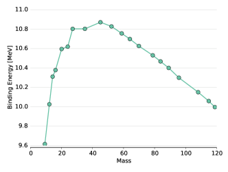
Figure 1: Binding energies of ground-state nuclei obtained with CMD model, extracted from Ref. Dorso et al. (2011).

II.2.2 Collisions

With respect to collisions, these potentials are known to reproduce nucleon-nucleon cross sections from low to intermediate energies Lenk et al. (1990), and it has been used extensively in studying heavy ion collisions (see Ref. Chernomoretz et al. (2002); Barrañón et al. (2007)). For such reactions, two “nuclei” are boosted against each other at a desired energy. From collision to collision, the projectile and target are rotated with respect to each other at random values of the Euler angles. The evolution of the system is followed using a velocity-Verlet algorithm with energy conservation better than 0.01%. At any point in time, the nucleon information, i.e., position and momenta, can be turned into fragment information by identifying the clusters and free particles; several such cluster recognition algorithms have been developed by our collaborator, C.O. Dorso, and they are well described in the literature Dorso and Aichelin (1995); Strachan and Dorso (1997).

The method yields mass multiplicities, momenta, excitation energies, secondary decay yields, etc. comparable to experimental data Belkacem et al. (1996); Chernomoretz et al. (2002). Figure 10, for instance, shows experimental and simulated parallel velocity distributions for particles obtained from mid-peripheral and peripheral ${}^{58}Ni+C$ collisions performed at the Coupled Tandem and Super-Conducting Cyclotron accelerators of AECL at Chalk River Chernomoretz et al. (2002).

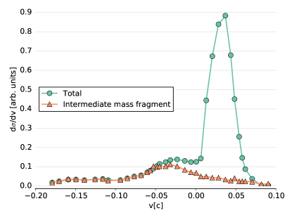
(a) $\eta=0.0001\,\text{fm/c}$

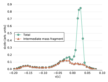
(b) $\eta=0.0001\,\text{fm/c}$

Figure 2: 2(a) Experimental and 2(b) simulated parallel velocity distributions for ${}^{58}Ni+C$ collisions.

II.2.3 Thermostatic Properties of Nuclear Matter

To study thermal properties of static nuclear matter, these drops or infinite systems, nucleons are positioned at random, but with a selected density, in a container and “heated”. After equilibration, the system can then be used to extract macroscopic variables. Repeating these simulations for a wide range of density and temperature values, information about the energy per nucleon, $\epsilon(\rho,T)$, can be obtained and used to construct analytical fits in the spirit of those pioneered by Bertsch, Siemens, and Kapusta Bertsch and J. Siemens (1983); Kapusta (1984); Lopez and Siemens (1984); these fits in turn can be used to derive other thermodynamic variables, such as pressure, etc.

Figure 3 shows the results of the method as applied by Giménez-Molinelli et al. Giménez Molinelli et al. (2014) for stiff cold infinite nuclear matter. The open symbols correspond to CMD calculations at low temperatures, showing a departure from the imposed homogeneous solutions obtained with the full symbols for different crystal symmetries. This shows the emergence of pseudo pastas in nuclear matter.

For finite systems, figure 4 demonstrates the feasibility of using CMD to study thermal properties such as the caloric curve (i.e. the temperature - excitation energy relationship) for a system of 80 nucleons equilibrated at four different densities; see Ref. Dorso et al. (2011) for complete details.

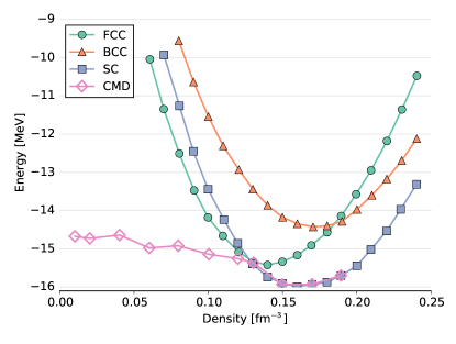
Figure 3: Nuclear matter energy per particle of cold matter calculated with CMD. Full symbols are for homogeneous systems, while open circles denote the emergence of the pseudo-pasta.

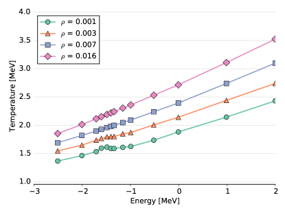
Figure 4: Caloric curve of a system equilibrated at four different densities calculated with CMD.

II.3 Coulomb interaction in the model

Since a neutralizing electron gas embeds the nucleons in the neutron star crust, the Coulomb forces among protons are screened. The model we used to model this screening effect is the Thomas-Fermi approximation, used with various nuclear models Maruyama et al. (1998); Dorso et al. (2012); Horowitz et al. (2004b). According to this approximation, protons interact via a Yukawa-like potential, with a screening length $\lambda$:

$$V_{TF}(r)=q^{2}\frac{e^{-r/\lambda}}{r}.$$

Theoretical estimates for the screening length $\lambda$ are $\lambda\sim 100\,\text{fm}$ Fetter and Walecka (2003), but we set the screening length to $\lambda=20\,\text{fm}$. This choice was based on previous studies Alcain et al. (2014b), where we have shown that this value is enough to adequately reproduce the expected length scale of density fluctuations for this model, while larger screening lengths would be a computational difficulty. We analyze the opacity to neutrinos of the structures for different proton fractions and densities.

III Neutron Star Matter at low densities and temperature

When we consider the system with a screened Coulomb interaction as described in II.3, a very interesting phenomena takes place, described with detail in Ref. Alcain et al. (2014b). At sub-saturation densities, the system displays an inhomogeneous structure known as nuclear pasta, characterized by the emergence of multiple structure per simulation cell, that can be roughly classified as gnocchi, spaghetti, lasagna and tunnels. As an example, in figure 5 we show the configurations of some of these pastas.

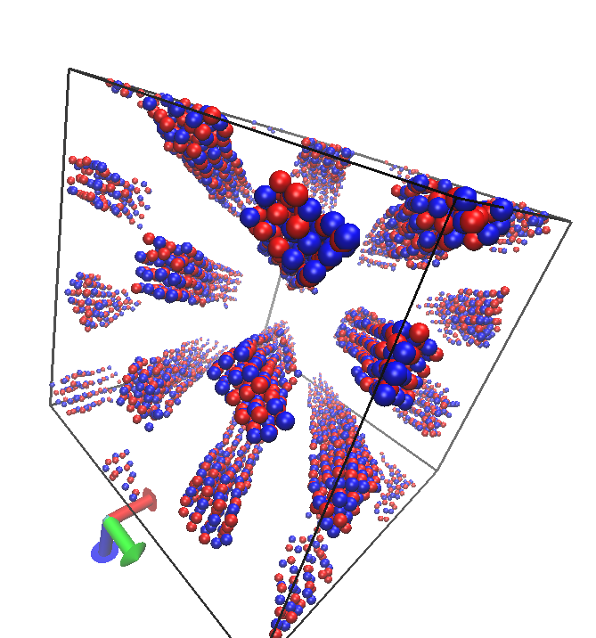
(a) $\rho=0.03\,\text{fm}^{-3}$

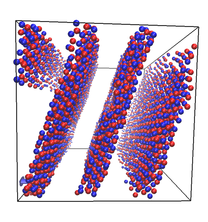
(b) $\rho=0.05\,\text{fm}^{-3}$

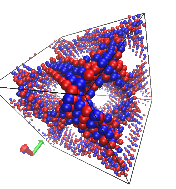
(c) $\rho=0.08\,\text{fm}^{-3}$

Figure 5: 5(a) Spaghetti, 5(b) lasagna and 5(c) tunnels obtained with the CMD method, for the symmetric case $x=0.5$ and low temperature $T=0.5\,\text{MeV}$ extracted from Ref. Alcain et al. (2014b)

IV Expansion

To simulate an expanding system we scale linearly with time the length of the box in every dimension,

$$L(t)=L_{0}(1+\eta\,t)$$

This, however, is not enough to expand the system collectively. We also need the particles inside the cell to expand like the box. In order to accomplish this, based on Ref. Dorso and Strachan (1996), we add to each particle a velocity $v_{exp}$ dependent on the position in the box:

$$\mathbf{v_{exp}}=\eta\,\mathbf{r}$$

We can see from this expression that the particles in the edge of the box will have an expanding velocity equal to that of the box.

Another effect to consider of this expansion is that when a particle crosses a boundary its velocity has to change according to the velocity of the expanding box. For example, if the particle crosses the left-hand boundary of the periodic box, the velocity of the image particle $v_{i}^{\dagger}$ on the right-hand must be modified $v_{i}^{\dagger}=v_{i}+L_{0}\,\eta$.

V Cluster recognition

In typical configurations we have not only the structure known as nuclear pasta, but also a nucleon gas that surrounds the nuclear pasta. In order to properly characterize the pasta phases, we must know which particles belong to the pasta phases and which belong to this gas. To do so, we have to find the clusters that are formed along the simulation.

One of the algorithms to identify cluster formation is Minimum Spanning Tree (MST). In MST algorithm, two particles belong to the same cluster $\{C^{\text{MST}}_{n}\}$ if the relative distance of the particles is less than a cutoff distance $r_{cut}$:

$$i\in C^{\text{MST}}_{n}\Leftrightarrow\exists j\in C_{n}\mid r_{ij}<r_{cut}$$

This cluster definition works correctly for systems with no kinetic energy, and it is based in the attractive tail of the nuclear interaction. However, if the particles have a non-zero temperature, we can have a situation of two particles that are closer than the cutoff radius, but with a large relative kinetic energy.

To deal with situations of non-zero temperatures, we need to take into account the relative momentum among particles. One of the most sophisticated methods to accomplish this is the Early Cluster Recognition Algorithm (ECRA) Dorso and Randrup (1993). In this algorithm, the particles are partitioned in different disjoint clusters $C^{\text{ECRA}}_{n}$, with the total energy in each cluster:

$$\epsilon_{n}=\sum_{i\in C_{n}}K^{CM}_{i}+\sum_{i,j\in C_{n}}V_{ij}$$

where $K^{CM}_{i}$ is the kinetic energy relative to the center of mass of the cluster. The set of clusters $\{C_{n}\}$ then is the one that minimizes the sum of all the cluster energies $E_{\text{partition}}=\sum_{n}\epsilon_{n}$.

ECRA algorithm can be easily used for small systems Dorso and Balonga (1994), but being a combinatorial optimization, it cannot be used in large systems. While finding ECRA clusters is very expensive computationally, using simply MST clusters can give extremely biased results towards large clusters. We have decided to go for a middle ground choice, the Minimum Spanning Tree Energy (MSTE) algorithm Dorso et al. (2012). This algorithm is a modification of MST, taking into account the kinetic energy. According to MSTE, two particles belong to the same cluster $\{C^{\text{MSTE}}_{n}\}$ if they are energy bound:

$$i\in C^{\text{MSTE}}_{n}\Leftrightarrow\exists j\in C_{n}:V_{ij}+K_{ij}\leq 0$$

While this algorithm doesn’t yield the same theoretically sound results from ECRA, it still avoids the largest pitfall of naïve MST implementations for the temperatures used in this work.

V.1 Infinite Clusters

We developed an algorithm for the recognition of infinite clusters across the boundaries. We explain here in detail the implementation for MST clusters in 2D, being the MSTE and 3D extension straightforward. In figure 6 we see a schematical representation of 2D clusters recognized in a periodic cell, labeled from 1 to 6 (note that these clusters don’t connect yet through the periodic walls).

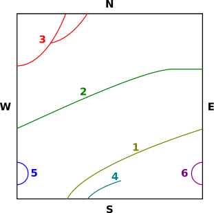
Figure 6: (Color online) Schematical representation of 2D clusters, recognized only in the cell and not through the periodic walls, labeled as N, S, W, E. The clusters inside the cell are labeled from 1 to 6,

In order to find the connections of these clusters through the boundaries, we draw a labeled graph of the clusters, where we connect clusters depending on whether they connect or not through a wall and label such connection with the wall label. For example, we begin with cluster 1. It connects with cluster 2 going out through the E wall, therefore we add a $1\rightarrow 2$ connection labeled as E. Symmetrically, we add a $2\rightarrow 1$ connection labeled as W. Now we go for the pair 1-3. It connects going out through the S wall, so we add $1\rightarrow 3$ labeled as S and $3\rightarrow 1$ labeled as N. Cluster 1 does not connect with 4, 5, or 6, therefore those are the only connections we have. Once we’ve done that, we get the graph of figure 7.

Figure 7: Graph of the clusters with connections labeled by the wall of the boundary they connect through. The graph can be divided in 2 subgraphs that don’t connect: 1–2–3–4 and 5–6. Each of these subgraphs is as cluster when periodic boundary conditions are considered.

We now wonder whether these subgraphs represent an infinite cluster or not not. In order to have an infinite clusters, we need to have a loop (the opposite is not true: having a loop is not enough to have an infinite cluster, as we can see in subragph 5–6), so we first identify loops and mark them as candidates for infinite clusters. Every connection adds to a loop (since the graph connections are back and forth), but we know from inspecting the figure 7 that the cluster 1–2–3 is infinite. Finding out what makes, in the graph, the cluster 1–2–3 infinite is key to identify infinite clusters. And the key feature of cluster 1–2–3 is that its loop 1–2–3–1 can be transversed through the walls E–E–S, while loops like 5–6 can be transversed only through E–W. Now, in order for the cluster to be infinite, we need it to extend infinitely in (at least) one direction. So once we have the list of walls of the loop, we create a magnitude I associated to each loop that is created as follows: beginning with $I=0$, we add a value $M_{i}$ if there is (at least one) $i$ wall. The values are: $M_{E}=1$, $M_{W}=-1$, $M_{N}=2$, $M_{S}=-2$. If $I$ is nonzero, then the loop is infinite. For example, for the loop E–E–S, we have E and S walls, so $I=M_{E}+M_{S}=3$ and the loop is infinite. For the loop E–W, $I=M_{E}+M_{W}=0$, and the loop is finite.

VI Results

In figure 8 we show the initial and final states for the expansion of $N=11000$ particle primordial cell (see caption for details) for the case of low velocity expansion. It can be immediately seen that though the initial configuration shows a compact particle distribution, the final configuration consists of gnocchi structures (almost spherical fragments) with a mass of about 80 particles.

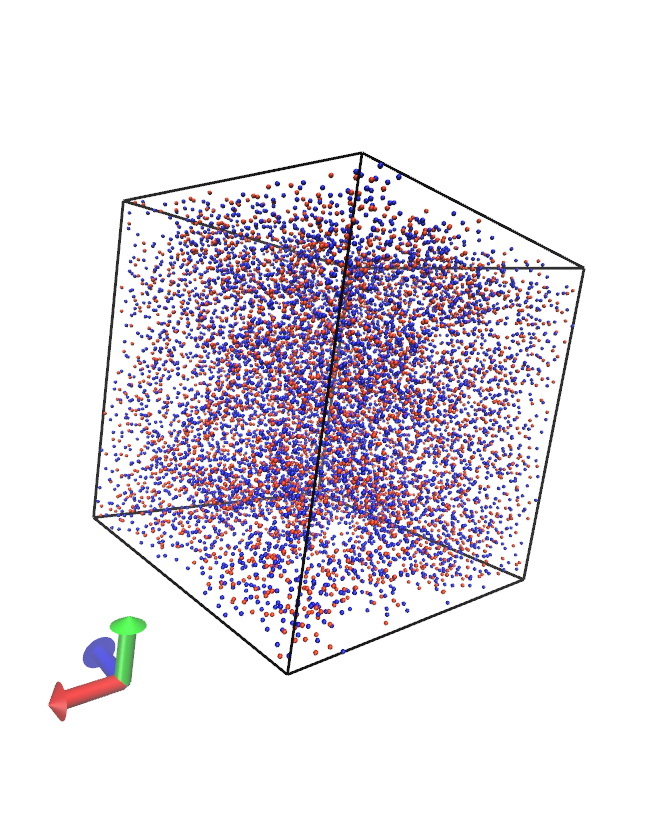
(a) $\eta=0.0001\,\text{fm/c}$

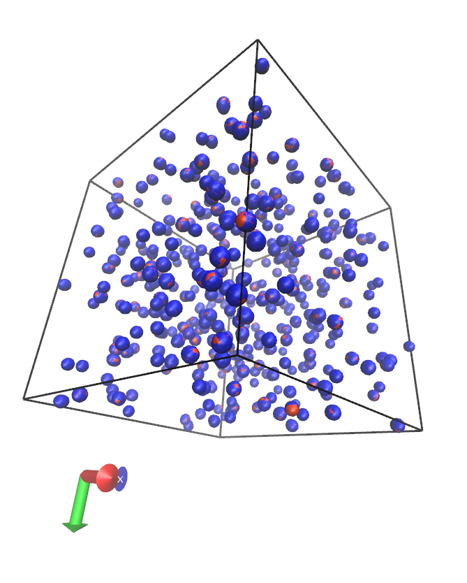
(b) $\eta=0.0005\,\text{fm/c}$

Figure 8: (Color online) Snapshots of a system in the initial configuration 8(a) and the final expanded system 8(b). In the expanded system we see clearly formed gnocchi clusters

In figure 9 we show the fraction of particles in the primordial cell that form part of an infinite cluster (Infinite Fragment Fraction, IFF). It can be easily seen that in the early stages of the evolution, due to the fact that the temperature is low, most of the system in the primordial cell belongs to the infinite clusters. But as the system evolves according to the expansion rate as explained above, the IFF goes down and goes to zero rather quickly, meaning that there is no more infinite fragment in the system. See caption for details.

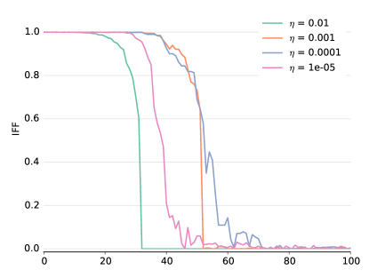
Figure 9: (Color online) Infinite Fragment Fraction (see text) as a function of the length of the edge of the primordial cell. For every expansion rate displayed the IFF goes to zero in the asymptotic regime.

Figure 10 shows the asymptotic fragment mass distribution for 4 different expansion rates. In this case, the MSTE algorithm has been applied over the primordial cell, taking into account periodic boundary conditions knowing that there is no infinite fragment as shown in figure 9. It can be seen that as the homogeneous expansion velocity increases, the fragment mass distribution displays the familiar transition from U-shaped to exponential decay. Somewhere in between, a power law distribution is to be expected. In particular, figure 10(c) shows that with an expansion of $\eta=0.009\,\text{fm/c}$ we are close to a power law distribution. It is interesting to note that at variance with percolation or Lennard-Jones systems, due to the presence of the Coulomb long range repulsion term, it is not possible to see an infinite cluster in the asymptotic regime. Moreover, together with the rather large rate of expansion, we do not expect to find big clusters.

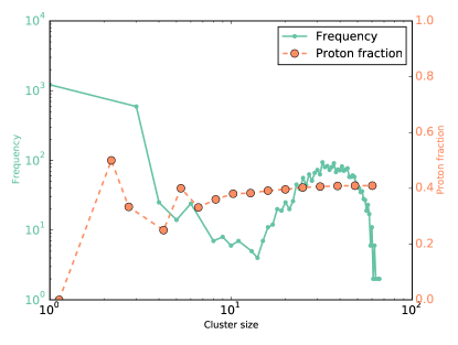
(a) $\eta=0.0001\,\text{fm/c}$

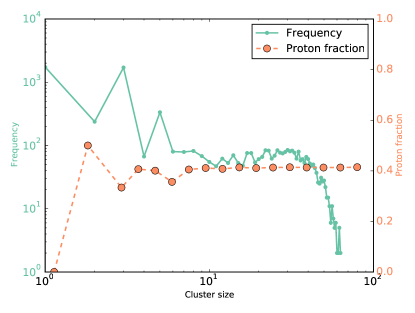
(b) $\eta=0.0005\,\text{fm/c}$

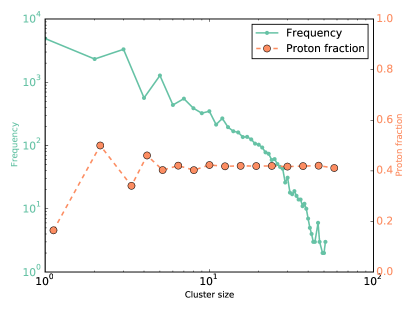
(c) $\eta=0.009\,\text{fm/c}$

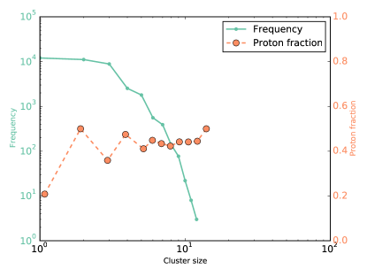
(d) $\eta=0.03\,\text{fm/c}$

Figure 10: (Color online) Fragment mass distribution. Labels grow with larger expansion rates. System consisting of 11000 particles with $x=0.4$ and initial density $\rho_{0}=0.08\,\text{fm}^{-3}$

VII Discussion and Concluding Remarks

In this work we have performed numerical experiments of homogeneously expanding systems with not very small amount of particles in the primordial cell. In order to analyze the fragment structure of such a system as a function of time, we have developed a graph-based tool for the identification of infinite fragments for any definition of percolation-like (i. e., additive) clusters. Once this formalism is applied to the above mentioned simulations, we have been able to identify the region in which a power-law distribution of masses is expected. The fragment mass distribution shapes range from U-like to exponential decay.

We are currently performing simulations with a larger number of particles to properly characterize the critical behavior of the system.

References

- Page et al. (2004) D. Page, J. M. Lattimer, M. Prakash, and A. W. Steiner, ApJS 155, 623 (2004).
- Geppert et al. (2004) U. Geppert, M. Küker, and D. Page, Astronomy & Astrophysics 426, 11 (2004).
- Woosley and Janka (2005) S. Woosley and T. Janka, Nature Physics 1, 147 (2005).
- Ravenhall et al. (1983) D. G. Ravenhall, C. J. Pethick, and J. R. Wilson, Phys. Rev. Lett. 50, 2066 (1983).
- Hashimoto et al. (1984) M.-a. Hashimoto, H. Seki, and M. Yamada, Prog. Theor. Phys. 71, 320 (1984).
- Williams and Koonin (1985) R. D. Williams and S. E. Koonin, Nuclear Physics A 435, 844 (1985).
- Oyamatsu (1993) K. Oyamatsu, Nuclear Physics A 561, 431 (1993).
- Lorenz et al. (1993) C. P. Lorenz, D. G. Ravenhall, and C. J. Pethick, Phys. Rev. Lett. 70, 379 (1993).
- Cheng et al. (1997) K. S. Cheng, C. C. Yao, and Z. G. Dai, Phys. Rev. C 55, 2092 (1997).
- Watanabe et al. (2000) G. Watanabe, K. Iida, and K. Sato, Nuclear Physics A 676, 455 (2000).
- Watanabe and Iida (2003) G. Watanabe and K. Iida, Phys. Rev. C 68, 045801 (2003).
- Nakazato et al. (2009) K. Nakazato, K. Oyamatsu, and S. Yamada, Phys. Rev. Lett. 103, 132501 (2009).
- Maruyama et al. (1998) T. Maruyama, K. Niita, K. Oyamatsu, T. Maruyama, S. Chiba, and A. Iwamoto, Phys. Rev. C 57, 655 (1998).
- Kido et al. (2000) T. Kido, T. Maruyama, K. Niita, and S. Chiba, Nuclear Physics A 663–664, 877c (2000).
- Watanabe et al. (2003) G. Watanabe, K. Sato, K. Yasuoka, and T. Ebisuzaki, Phys. Rev. C 68, 035806 (2003).
- Horowitz et al. (2004a) C. Horowitz, M. Pérez-García, J. Carriere, D. Berry, and J. Piekarewicz, Phys. Rev. C 70, 065806 (2004a).
- Dorso et al. (2012) C. O. Dorso, P. A. Giménez Molinelli, and J. A. López, Phys. Rev. C 86, 055805 (2012).
- Lenk et al. (1990) R. J. Lenk, T. J. Schlagel, and V. R. Pandharipande, Phys. Rev. C 42, 372 (1990).
- Dorso and Randrup (1988) C. Dorso and J. Randrup, Physics Letters B 215, 611 (1988).
- Alcain et al. (2014a) P. N. Alcain, P. A. Giménez Molinelli, and C. O. Dorso, Phys. Rev. C 90, 065803 (2014a).
- Bonasera et al. (2000) A. Bonasera, M. Bruno, C. O. Dorso, and F. Mastinu, (2000).
- Chikazumi et al. (2001) S. Chikazumi, T. Maruyama, S. Chiba, K. Niita, and A. Iwamoto, Phys. Rev. C 63, 024602 (2001).
- Caplan et al. (2015) M. E. Caplan, A. S. Schneider, C. J. Horowitz, and D. K. Berry, Phys. Rev. C 91, 065802 (2015).
- Lattimer and Schramm (1974) J. M. Lattimer and D. N. Schramm, The Astrophysical Journal Letters 192, L145 (1974).
- Goriely et al. (2011) S. Goriely, A. Bauswein, and H.-T. Janka, ApJ 738, L32 (2011).
- Barz et al. (1996) H. W. Barz, J. P. Bondorf, D. Idier, and I. N. Mishustin, Physics Letters B 382, 343 (1996).
- Nordheim (1928) L. W. Nordheim, Proceedings of the Royal Society of London. Series A 119, 689 (1928).
- Uehling and Uhlenbeck (1933) E. A. Uehling and G. E. Uhlenbeck, Phys. Rev. 43, 552 (1933).
- Polanski et al. (2005) A. Polanski, S. Petrochenkov, and V. Uzhinsky, Radiat Prot Dosimetry 116, 582 (2005).
- López and Dorso (2000) J. A. López and C. Dorso, Lectures Notes on Phase Transformations in Nuclear Matter (WORLD SCIENTIFIC, 2000).
- Chernomoretz et al. (2002) A. Chernomoretz, L. Gingras, Y. Larochelle, L. Beaulieu, R. Roy, C. St-Pierre, and C. O. Dorso, Phys. Rev. C 65, 054613 (2002).
- Barranon et al. (2001) A. Barranon, C. O. Dorso, and J. A. Lopez, Revista mexicana de física 47, 93 (2001).
- Dorso and López (2001) C. O. Dorso and J. A. López, Phys. Rev. C 64, 027602 (2001).
- Barranón et al. (2003) A. Barranón, R. Cárdenas, C. O. Dorso, and J. A. López, APH N.S., Heavy Ion Physics 17, 59 (2003).
- Barrañón et al. (2007) A. Barrañón, C. O. Dorso, and J. A. López, Nuclear Physics A 791, 222 (2007).
- Barrañón et al. (2004) A. Barrañón, J. Roa, and J. López, Phys. Rev. C 69, 014601 (2004).
- Dorso et al. (2006) C. O. Dorso, C. R. Escudero, M. Ison, and J. A. López, Phys. Rev. C 73, 044601 (2006).
- Dorso et al. (2011) C. A. Dorso, P. A. G. Molinelli, and J. A. López, J. Phys. G: Nucl. Part. Phys. 38, 115101 (2011).
- Plimpton (1995) S. Plimpton, Journal of Computational Physics 117, 1 (1995).
- Brown et al. (2012) W. M. Brown, A. Kohlmeyer, S. J. Plimpton, and A. N. Tharrington, Computer Physics Communications 183, 449 (2012).
- Dorso and Aichelin (1995) C. O. Dorso and J. Aichelin, Physics Letters B 345, 197 (1995).
- Strachan and Dorso (1997) A. Strachan and C. O. Dorso, Phys. Rev. C 55, 775 (1997).
- Belkacem et al. (1996) M. Belkacem, P. F. Mastinu, V. Latora, A. Bonasera, M. D’Agostino, M. Bruno, J. D. Dinius, M. L. Fiandri, F. Gramegna, D. O. Handzy, W. C. Hsi, M. Huang, G. V. Margagliotti, P. M. Milazzo, C. P. Montoya, G. F. Peaslee, R. Rui, C. Schwarz, G. Vannini, and C. Williams, Phys. Rev. C 54, 2435 (1996).
- Bertsch and J. Siemens (1983) G. Bertsch and P. J. Siemens, Physics Letters B 126, 9 (1983).
- Kapusta (1984) J. Kapusta, Phys. Rev. C 29, 1735 (1984).
- Lopez and Siemens (1984) J. A. Lopez and P. J. Siemens, Nuclear Physics A 431, 728 (1984).
- Giménez Molinelli et al. (2014) P. A. Giménez Molinelli, J. I. Nichols, J. A. López, and C. O. Dorso, Nuclear Physics A 923, 31 (2014).
- Horowitz et al. (2004b) C. J. Horowitz, M. A. Pérez-García, and J. Piekarewicz, Phys. Rev. C 69, 045804 (2004b).
- Fetter and Walecka (2003) A. L. Fetter and J. D. Walecka, Quantum Theory of Many-particle Systems (Courier Dover Publications, 2003).
- Alcain et al. (2014b) P. N. Alcain, P. A. Giménez Molinelli, J. I. Nichols, and C. O. Dorso, Phys. Rev. C 89, 055801 (2014b).
- Dorso and Strachan (1996) C. O. Dorso and A. Strachan, Phys. Rev. B 54, 236 (1996).
- Dorso and Randrup (1993) C. Dorso and J. Randrup, Physics Letters B 301, 328 (1993).
- Dorso and Balonga (1994) C. O. Dorso and P. E. Balonga, Phys. Rev. C 50, 991 (1994).