Abstract

We study the $(1,0)$ six-dimensional SCFTs living on defects of non-geometric heterotic backgrounds (T-fects) preserving a $E_{7}\times E_{8}$ subgroup of $E_{8}\times E_{8}$. These configurations can be dualized explicitly to F-theory on elliptic K3-fibered non-compact Calabi-Yau threefolds. We find that the majority of the resulting dual threefolds contain non-resolvable singularities. In those cases in which we can resolve the singularities we explicitly determine the SCFTs living on the defect. We find a form of duality in which distinct defects are described by the same IR fixed point. For instance, we find that a subclass of non-geometric defects are described by the SCFT arising from small heterotic instantons on ADE singularities.

1 Introduction

String theory admits a rich set of supersymmetric compactifications, giving rise to a vast space of lower dimensional field theories. Most of the study of these compactifications focuses on regimes where the background can be understood geometrically by considering a classical supergravity reduction on the geometry, supplemented with knowledge of the dynamics on brane stacks. This is far from being the only possibility, but it is very convenient and very amenable to concrete analysis. Nevertheless, it would be interesting to go away from this geometric class of backgrounds, both to learn more about the non-classical and non-geometrical properties of string theory, and to gain some insight about the broader set of possible string vacua.

In this paper we focus on a class of compactifications of the $E_{8}\times E_{8}$ heterotic string which are very non-classical, involving compactifications on “spaces” that cannot be globally described as geometries, while remaining accessible thanks to duality with F-theory. We can, in this way, probe many of the properties of the heterotic string away from the classical regime where it is conventionally studied.

More concretely, we will focus on cases where the compactification space for the heterotic string is at a generic point locally geometric, and described by a $T^{2}$ fibration. The non-classical nature of the background arises from the patching between local descriptions, which we choose to involve non-trivial elements of the T-duality group acting on the $T^{2}$ [1]. The resulting total space is usually referred to as a non-geometric T-fold [2]. In the context of the heterotic string one should note that there is additional gauge bundle data (denoted by $E_{T^{2}}$ in the following) which mixes with the geometric data of the $T^{2}$ under generic elements of the T-duality group of the $T^{2}$. The patching will send $(\tau,\rho,E_{T^{2}})\to(\tau^{\prime},\rho^{\prime},E^{\prime}_{T^{2}})$, with $\tau$ the complex structure of the torus, $\rho=\int_{T^{2}}B+iJ$ its complexified Kähler modulus, and $E_{T^{2}}$ the Wilson line data along the two cycles of the torus. The primed values arise from the action of the $O(2,18,\mathbb{Z})$ T-duality on the $T^{2}$.

Such fibrations will in general have defects, i.e. subloci of the compactification space where a local description in terms of the heterotic string on a smooth $T^{2}\times\mathbb{R}^{n}$ with a smooth bundle is no longer possible. For concreteness, we consider the compactification of the heterotic string to six dimensions. In this case, we have locally a $T^{2}$ fibration over a complex one-dimensional base. At certain points of the base we have defects, which will induce a monodromy action on $(\tau,\rho,E_{T^{2}})$ as we go around them. Our goal in this paper is to describe, for a particular class of bundles $E_{T^{2}}$, the low energy dynamics living on the defect itself.

We will do this by dualizing the configuration to F-theory, where the dynamics on the defect can be characterized by purely geometric means. In order to do so in the most explicit way possible, we restrict the bundle $E_{T^{2}}$ to have $SU(2)$ structure, so it will break $E_{8}\times E_{8}$ down to $E_{8}\times E_{7}$. The bundle data on the $T^{2}$ is then described by a single complex number, whose real and imaginary parts are given by the Wilson line of the $SU(2)$ Cartan around the one-cycles of the $T^{2}$. We denote this complexified Wilson line by $\beta$ in the rest of the paper.

With a single Wilson line turned on, the T-duality group is $O(2,3,\mathbb{Z})$ and an order four subset of this group can be identified with $Sp(4,\mathbb{Z})$, which is the action of the mapping class group of a genus-two curve on the homology. In this paper we restrict to monodromies in this $Sp(4,\mathbb{Z})$ subgroup, so we have a formulation in terms of monodromies of genus-two curves. This correspondence is in fact very deep: as shown recently in [3, 4], there is a very close connection between the moduli space of genus-two Riemann surfaces and the moduli space of elliptically fibered K3 surfaces having an $E_{8}$ and an $E_{7}$ point. By duality with F-theory, this is precisely the moduli space of the heterotic string on $T^{2}$ with a single Wilson line. Furthermore, the map has been explicitly worked out in [6, 7, 4, 8] (generalizing previous work in the case with unbroken $E_{8}\times E_{8}$ symmetry [9, 3]): given a genus-two Riemann surface, parameterizing the moduli of a heterotic compactification with unbroken $E_{8}\times E_{7}$, there are explicit expressions — to be reviewed below — for the moduli of the dual K3.

In fact, the existence of the genus-two description for the heterotic vacua on $T^{2}$ with a single Wilson line gives us a formal, but geometric, description of the very non-geometric heterotic compactifications of interest in this paper. This viewpoint is particularly fruitful since there exists a classification of the possible degenerations of genus-two fibers over a complex one-dimensional base, obtained by Ogg-Namikawa-Ueno [10, 11]. This is analogous to, but more involved than, the Kodaira classification of degenerations of genus one fibrations, which are extensively used in F-theory.

We can now summarize the main results of this paper. For each of the possibilities allowed by the classification of genus-two degenerations — or equivalently, for every defect preserving $E_{8}\times E_{7}$ and with monodromy in $Sp(4,{\mathbb{Z}})$ — we will apply the heterotic/F-theory duality map to express the heterotic backgrounds in terms of F-theory compactifications. Generically, the F-theory background dual to a given 5-brane defect on the heterotic side will be highly singular. In some cases (the exact criterion is stated in section 6) we can resolve the singularity by performing a finite number of blow-ups in the base of the fibration. For all the cases where this resolution is possible we construct the resulting smooth geometry. The blow-ups correspond to giving vevs to tensor multiplets of the 6d (1,0) theory on the defect, such that it flows to a Lagrangian description in the IR. In this way, from the knowledge of the smooth geometry one can understand some aspects (such as anomaly polynomials [12, 13]) of the strongly coupled CFT living at the origin of the tensor branch in terms of more ordinary quantum field theories. Let us note that as one might have expected, for the cases that we can resolve we obtain theories that fall into the recent classification of [14, 15, 16].

In order to test our approach we will first consider local genus-two models that correspond to geometric ADE singularities of a K3 surface, together with a monodromy $\rho\rightarrow\rho+n$ for the complexified Kähler modulus. As expected, from the resolution of the dual F-theory models we find a non-perturbative enhancement of the gauge algebra which agrees with the theory of pointlike instantons hitting the orbifold singularity determined in [17], with $n$ related to the number of instantons at the singular point ($n=0$ corresponds to local cancellation of the modified Bianchi identity, and thus to having as many small instantons as the degree of the ADE singularity). We also determine the matter content from the dual F-theory geometry, and verify explicitly that it agrees with the expectation from anomaly cancellation [18].

We then move on to non-geometric models that involve monodromies in the Kähler modulus $\rho$ with a non-trivial action on the torus volume. We find a form of duality, in that distinct defects can give rise to the same SCFTs. For instance, we often encounter the same SCFTs as those describing pointlike instantons on ADE singularities, even for defects arising from non-geometric configurations. Understanding the origin of these dualities is an important open problem. We stress that we also find non-geometric degenerations which are not dual to pointlike instantons on ADE singularities, and give SCFTs which are genuinely new in the heterotic context.

This paper is organized as follows. In section 2 we review the formulation of heterotic/F-theory duality in terms of a map between genus-two curves and K3 surfaces, and we discuss how it can be used to study non-geometric heterotic backgrounds in terms of K3 fibered Calabi-Yau three-folds. In section 3 we apply our formalism to study local heterotic degenerations which admit a geometric description in some duality frame. In section 4 we discuss truly non-geometric models and we show how to construct a global model with such degenerations. We also explicitly describe various dualities between different non-geometric and geometric defects. In section 5 we list the resolutions of the remaining non-geometric models, considering in particular a class of models that do not admit a limit with vanishing Wilson line. Finally in section 6 we provide the details of the classification of all possible local heterotic models, both geometric and non-geometric, admitting F-theory duals that can be resolved into smooth Calabi-Yau three-folds. We conclude with a discussion in section 7. We relegate to appendix A the resolutions of geometric models that correspond to pointlike instantons on ADE singularities. In appendix B we discuss the heterotic/F-theory duality for the case of vanishing Wilson line. In appendix C we show the expressions of the Igusa-Clebsch invariants in terms of coefficients of a sextic that describe a given genus-two curve. In appendix D we reproduce the Namikawa-Ueno classification of singular genus-two fibers, and for each entry we compute the order of vanishing of the Igusa-Clebsch invariants. Finally, in appendix LABEL:sec:matter-analysis we explain how to extract the matter content from the F-theory resolutions for an explicit example.

2 Non-geometric heterotic vacua

In this section we review the formulation of F-theory/heterotic duality recently discussed in [4, 8]. We first discuss the duality in eight dimensions and then we show how to fiber it over a common base to study non-geometric heterotic compactifications to six-dimensions in terms of F-theory on Calabi-Yau three-folds.

2.1 Heterotic/F-theory duality in 8 dimensions

It is well known that the $E_{8}\times E_{8}$ heterotic string compactified on ${\rm T}^{2}$ is dual to F-theory compactified on an elliptically fibered K3 surface [19]. For the heterotic compactification with a Wilson line that breaks the gauge group to $E_{7}\times E_{8}$ the corresponding K3 is described by a Weierstraß model of the form

$$y^{2}=x^{3}+(a\,u^{4}v^{4}+c\,u^{3}v^{5})\,x\,w^{4}+(b\,u^{6}v^{6}+d\,u^{5}v^{7}+u^{7}v^{5})\,w^{6}=0\,,$$ (2.1)

where $[u:v]\in{\mathbb{P}}^{1}$ and $[y:x:w]\in{\mathbb{P}}_{3,2,1}$ are the homogeneous coordinates of the base and the Weierstraß equation, respectively. For generic values of the coefficients the fiber has a Kodaira singularity of type $\mathrm{III^{*}}$ ($E_{7}$) at $u=0$ and a singularity of type $\mathrm{II^{*}}$ ($E_{8}$) at $v=0$. By virtue of the F-theory/heterotic duality, there must be a map relating the heterotic moduli $\rho$, $\tau$ and $\beta$ to the K3 coefficients $a$, $b$, $c$ and $d$.

To obtain an understanding for this map, we study certain limits thereof. Consider first the special case $c=0$. One can immediately see from (2.1) that this implies that both singularities are of type $\mathrm{II^{*}}$ ($E_{8}$). Thus, $c=0$ corresponds to vanishing Wilson line, i.e. to $\beta=0$. In this limit, the coefficients $a$, $b$ and $d$ are related to the heterotic moduli $\tau$ and $\rho$ in the following way

$$j(\tau)j(\rho) =-1728^{2}\frac{a^{3}}{27d}\,,$$ (2.2)

$$(j(\tau)-1728)(j(\rho)-1728) =1728^{2}\frac{b^{2}}{4d}\,,$$

where $j$ is the $SL(2,\mathbb{Z})$ modular invariant function. The map for this specific configuration was originally obtained in [9]. Note that we can interpret the moduli $\tau$ and $\rho$ as complex structures of two elliptic curves (one of which is the physical heterotic torus) which are glued together at one point, i.e. a degenerated genus-two curve. The map thus can be read as a relation between $SL(2,\mathbb{Z})$ modular forms and the K3 coefficients, cf. appendix B. As we will now discuss, we can extend this relation to encompass a non-vanishing Wilson line.

In the general setup, with $c\neq 0$, the map has been recently established in [4], using previous findings about K3 surfaces related to curves of genus two [20, 21, 7]. The three heterotic complex parameters $\rho$, $\tau$, $\beta$ live on the Narain moduli space

$${\mathcal{M}}_{\rm het}={\mathcal{D}}_{2,3}/O(2,3,{\mathbb{Z}})\qquad\textmd{with}\qquad{\mathcal{D}}_{2,3}:=\frac{O(2,3,{\mathbb{R}})}{O(2,{\mathbb{R}})\times O(3,{\mathbb{R}})}\,,$$ (2.3)

where we used the notation of [4]. We will consider a subset $O^{+}(L^{2,3})$ of the Narain U-duality group $O(2,3,{\mathbb{Z}})$ which preserves orientations, because we will be ultimately interested in fibering the duality group holomorphically over a base.

A crucial observation is that there is an isomorphism ${\mathcal{D}}_{2,3}\cong{\mathbb{H}}_{2}$ between the symmetric space and the genus-two Siegel upper half-plane [22]:

$${\mathbb{H}}_{2}=\left\{\Omega=\left(\!\!\begin{array}[]{cc}\tau&\beta\\ \beta&\rho\end{array}\!\!\right)\bigg{|}\ \tau,\rho,\beta\in{\mathbb{C}},\ \det{\rm Im\,}(\Omega)>0,\ {\rm Im\,}(\rho)>0\right\}\,.$$ (2.4)

Since on the same grounds a (two-to-one) relation between $O^{+}(L^{2,3})$ and $Sp(4,{\mathbb{Z}})$ can be established, there is a correspondence between the moduli space of the heterotic compactification and the quotient of ${\mathbb{H}}_{2}$ by the genus-two modular group $Sp(4,{\mathbb{Z}})$. The action of $M\in Sp(4,{\mathbb{Z}})$ on $\Omega$ is given by

$$M(\Omega)=(A\Omega+B)(C\Omega+D)^{-1}\,,\quad M=\left(\!\!\begin{array}[]{cc}A&B\\ C&D\end{array}\!\!\right)$$ (2.5)

where $A$, $B$, $C$ and $D$ are $2\times 2$ matrices such that $M\in Sp(4,{\mathbb{Z}})$. More details about this quotient and the relation to ${\mathcal{M}}_{\rm het}$ can be found in [4] and [22].

A genus-two curve has four linearly independent cycles that can be chosen to span a canonical basis such that the intersection form has a symplectic structure (see e.g. [23]). We indicate the symplectic basis as $(a_{1},a_{2},b_{1},b_{2})$ in figure 1. The matrix $\Omega$ introduced in eq. (2.4) can be determined from integrals of the two holomorphic one-forms over the $a_{i}$, $b_{i}$ cycles [11]. The transformations in $Sp(4,{\mathbb{Z}})$ are induced by changes of homology basis that preserve the intersection form.

Coming back to the dual F-theory description (2.1), it has been found that the duality map can be expressed in terms of genus-two Siegel modular forms as [20, 21, 7, 4]

$$a=-\frac{1}{48}\psi_{4}(\Omega)\,,\quad b=-\frac{1}{864}\psi_{6}(\Omega)\,,\quad c=-4\chi_{10}(\Omega)\,,\quad d=\chi_{12}(\Omega)\,.$$ (2.6)

The definition and properties of the relevant Siegel modular forms can be found in [4], see also [8].

We also note that in eight dimensions the heterotic/F-theory map we use naturally geometrizes the extra massless string states appearing at self-dual points on the moduli space in terms of degenerations of the dual K3 surface [9, 24]. A recent discussion on this from the double field theory point of view appeared in [25].

Genus-two curves

As we have discussed above, the heterotic moduli can be put in correspondence with the moduli of a hyperelliptic genus-two curve. In turn such curve, denoted $\Sigma$, can be represented by a sextic:

$$y^{2}=f(x)=\sum_{i=0}^{6}c_{i}\,x^{i}=c_{6}\prod_{i=1}^{6}(x-\theta_{i})\,.$$ (2.7)

In order to connect the $c_{i}$ coefficients with the $a$, $b$, $c$, $d$ in the dual K3 fibration (2.1), we need to determine the Siegel modular forms appearing in the map (2.6) in terms of the $c_{i}$’s. This can be done in a convenient way by first computing the Igusa-Clebsch invariants of the sextic (2.7) and then relating them to the Siegel modular forms of the corresponding genus-two curve. The Igusa-Clebsch invariants are defined in terms of the six roots $\theta_{i}$ of (2.7) as:

$$\begin{split}I_{2}&=c_{6}^{2}\sum_{15}(12)^{2}(23)^{2}(45)^{2}\,,\\ I_{4}&=c_{6}^{4}\sum_{10}(12)^{2}(23)^{2}(31)^{2}(45)^{2}(56)^{2}(64)^{2}\,,\\ I_{6}&=c_{6}^{6}\sum_{60}(12)^{2}(23)^{2}(31)^{2}(45)^{2}(56)^{2}(64)^{2}(14)^{2}(25)^{2}(36)^{2}\,,\\ I_{10}&=c_{6}^{10}\prod_{i<j}(ij)^{2}\,,\end{split}$$ (2.8)

where $(ij):=(\theta_{i}-\theta_{j})$ and the sums are over permutations [26]. By using a computer algebra program, we find the general expressions for $I_{2}$, $I_{4}$, $I_{6}$, $I_{10}$ as functions of the coefficients $c_{i}$ of the sextic (2.7). These are somewhat involved and are therefore relegated to appendix C.

In the case of a genus-one curve, the discriminant, as well as the coefficients, of the Weierstraß cubic, are related to $SL(2,{\mathbb{Z}})$ modular forms with argument the modular parameter $\tau$ of the genus-one curve. For a curve of genus-two the Igusa-Clebsch invariants are similarly given by Siegel modular forms as follows [26]:

$$I_{2}(c_{i})=\frac{\chi_{12}(\Omega)}{\chi_{10}(\Omega)}\,, I_{4}(c_{i})=2^{-4}\cdot 3^{-2}\psi_{4}(\Omega)\,,$$ (2.9)

$$I_{6}(c_{i})=2^{-6}\cdot 3^{-4}\psi_{6}(\Omega)+2^{-4}\cdot 3^{-3}\frac{\psi_{4}(\Omega)\chi_{12}(\Omega)}{\chi_{10}(\Omega)}\,, I_{10}(c_{i})=2^{-1}\cdot 3^{-5}\chi_{10}(\Omega)\,,$$

with $\Omega$ specified by the three complex moduli of the genus-two curve. From (2.6) we can write the dual K3 coefficients in terms of the Igusa-Clebsch invariants and thus in terms of polynomials of the coefficients $c_{i}$:

$$a=-3I_{4}\,,\quad b=2(I_{4}I_{2}-3I_{6})\,,\quad c=-2^{3}3^{5}I_{10}\,,\quad d=2\,3^{5}I_{2}I_{10}\ .$$ (2.10)

This form of the map will be very important for the purpose of studying non-geometric heterotic vacua in lower dimensions.

2.2 From 8 to 6 dimensions: local models and exotic defects

In the previous section we reviewed the close relation between the moduli space of the heterotic string on $T^{2}$ with one complex Wilson line and the moduli spaces of genus-two curves and elliptically fibered K3 surfaces developing $E_{7}\times E_{8}$ degenerations. This led to a formulation of F-theory/heterotic duality which is very useful once we consider compactifications to lower dimensions, obtained by allowing the moduli to vary along a (compact) base variety $\mathcal{B}$. We are interested in the case were $\mathcal{B}$ is complex one-dimensional, locally parametrized by a complex coordinate $t\in{\mathbb{C}}$. The structure of such a compactification is that of a fibration, with fiber a point in the Narain space or equivalently a genus-two curve which encodes this point and the base given by $\mathcal{B}$. Such fibrations allow for a varying $\Omega(t)$ with $Sp(4,{\mathbb{Z}})$ identifications at chart transitions, or to be more precise along non-contractible loops. Since every consistent genus-two fibration will give us a consistent fibration of $\Omega(t)$, we will restrict our attention in the following to the first one. This has the advantage that we obtain again a geometry with which we can more easily deal.

To preserve supersymmetry this fibration has to be holomorphic. In the case of a non-trivial fibration this implies that the genus-two curve $\Sigma(t)$ has to degenerate at co-dimension one loci on the base. Moreover, following $\Omega(\Sigma(t))$ of the genus-two curve around such a degeneration locus it will experience a monodromy transformation. Since along a loop we end up with the same fiber that we started with, the monodromy must belong to $Sp(4,\mathbb{Z})$. Hence, the moduli fields of the heterotic $T^{2}$ compactification equal only modulo a duality transformation when we go around such a non-trivial loop. Since the duality group includes transformations of the type $\rho\to-1/\rho$, thereby exchanging small and large volume, the spaces around such singularities are in general non-geometric T-folds. Note that the non-geometric structure is here of global kind, i.e. as long as we are probing only the local neighborhood of a regular point we do not experience any duality transformations.

In order to get some intuition regarding $\rho$ degenerations, let us consider the monodromy $\rho\to\rho+1$. This arises around a point $t_{0}\in\mathcal{B}$ at which the cycle $a_{2}$ of $\Sigma$ shrinks, cf. figure 1. The monodromy corresponds to a Dehn twist around this vanishing cycle. In this case the singularity can be identified with a NS5-brane [27]. In fact, the corresponding solution $\rho(t)=1/(2\pi i)\log(t-t_{0})$ coincides with the solution for a NS5-brane on $\mathbb{C}\times T^{2}$ if one neglects its position on the $T^{2}$. By pinching a different cycle, i.e. $p\,a_{2}+q\,b_{2}$, one gets a more general $(p,q)$ monodromy in $\rho$, with solution (for $q\neq 0$):

$$\rho(t)=-\frac{2\pi i}{q^{2}\log\left(t-t_{0}\right)}-\frac{p}{q}\,.$$ (2.11)

As an example, we can consider the monodromy $\rho\rightarrow\rho/(1-\rho)$, corresponding to a $(0,1)$ degeneration. The volume of the fiber does not come back to itself after encircling the defect, and hence the solution is non-geometric. It coincides with an exotic $5^{2}_{2}$-brane (or Q-brane) [28, 29, 30].

More general, as in F-theory, one can have $\rho$ degenerations described by monodromies in different conjugacy classes of the duality group. The typical genus-two degeneration will induce also monodromies for the moduli $\tau$ and $\beta$. As in[31], we refer to such degenerations as T-duality defects, or T-fects. The aim of this paper is to uncover the six-dimensional theories that live on such T-fects.

An advantage of mapping the non-geometric fibrations to geometric genus-two fibrations is the existence of a classification of all possible local degenerations of genus-two fibers due to Ogg and Namikawa-Ueno (NU) [10, 11]. This is analogous to the Kodaira classification of genus-one curves [32] which we reproduce in table 1. Furthermore, NU give explicit local descriptions of the possible degenerations in terms of hyperelliptic curves. Our strategy will be then to compute the Igusa-Clebsch invariants for each local genus-two model that realizes a given $Sp(4,\mathbb{Z})$ monodromy, and use the F-theory/heterotic map (2.10) to obtain the corresponding K3 degeneration in the dual F-theory model.

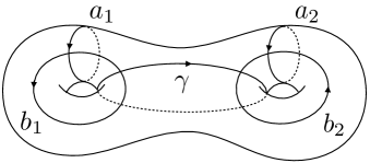
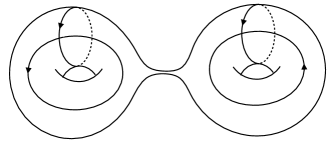
Figure 1: (a) The Humphries generators for a genus-two surface $\Sigma$: any element of the mapping class group $\mathcal{M}(\Sigma)$ can be written as a product of Dehn twists along the cycles $(a_{1},b_{1},\gamma,a_{2},b_{2})$. Note that $\gamma=a_{1}^{-1}a_{2}$. (b) Switching off the Wilson line parameter $\beta$ corresponds to splitting $\Sigma$ into two genus-one components. This geometrizes the $SL(2,\mathbb{Z})_{\tau}\times SL(2,\mathbb{Z})_{\rho}$ subgroup of the T-duality group $O(2,2,\mathbb{Z})$.

In the following we briefly describe the structure of the NU list for genus-two degenerations. For the reader’s convenience, we reproduce this list in appendix D (and adopt their notation). For each model we list the order of vanishing of the Igusa-Clebsch invariants that we compute from the expressions (C.1)-(C.4).

The geometric picture is especially useful to understand the different classes of degenerations and to obtain a decomposition of the monodromies in terms of a set of generators, in analogy with the ABC factorization of F-theory [33, 34]. It follows from a theorem of Humphries (see for instance [35]) that the mapping class group of $\Sigma$ is generated by Dehn twists along the set of five cycles $(a_{1},b_{1},\gamma,a_{2},b_{2})$, shown in figure 1. If we pick the base $\mathtt{B}=(a_{1},a_{2},b_{1},b_{2})$ for $H_{1}(\Sigma,\mathbb{Z})$, their symplectic representation is:

$$\begin{split}A_{1}&=\begin{pmatrix}1&0&1&0\\ 0&1&0&0\\ 0&0&1&0\\ 0&0&0&1\end{pmatrix}\,,\quad B_{1}=\begin{pmatrix}1&0&0&0\\ 0&1&0&0\\ -1&0&1&0\\ 0&0&0&1\end{pmatrix}\,,\quad\Gamma=\begin{pmatrix}1&0&1&-1\\ 0&1&-1&1\\ 0&0&1&0\\ 0&0&0&1\end{pmatrix}\,,\\[10.0pt] A_{2}&=\begin{pmatrix}1&0&0&0\\ 0&1&0&1\\ 0&0&1&0\\ 0&0&0&1\end{pmatrix}\,,\quad B_{2}=\begin{pmatrix}1&0&0&0\\ 0&1&0&0\\ 0&0&1&0\\ 0&-1&0&1\end{pmatrix}\,.\end{split}$$ (2.12)

The action of these $Sp(4,\mathbb{Z})$ elements on the period matrix defined by (2.5) gives the following monodromies for the moduli:

$$\begin{split}A_{1}&:\quad\tau\rightarrow\tau+1\,,\quad\rho\rightarrow\rho\,,\quad\beta\rightarrow\beta\,,\\ B_{1}&:\quad\tau\rightarrow\frac{\tau}{1-\tau}\,,\quad\rho\rightarrow\rho+\frac{\beta^{2}}{1-\tau}\,,\quad\beta\rightarrow\frac{\beta}{1-\tau}\,,\\ \Gamma&:\quad\tau\rightarrow\tau+1\,,\quad\rho\rightarrow\rho+1\,,\quad\beta\rightarrow\beta-1\,,\\ A_{2}&:\quad\tau\rightarrow\tau\,,\quad\rho\rightarrow\rho+1\,,\quad\beta\rightarrow\beta\,,\\ B_{2}&:\quad\tau\rightarrow\tau+\frac{\beta^{2}}{1-\rho}\,,\quad\rho\rightarrow\frac{\rho}{1-\rho}\,,\quad\beta\rightarrow\frac{\beta}{1-\rho}\,.\end{split}$$ (2.13)

Note that when $\beta=0$, $\Sigma$ splits into the two genus-one components whose mapping class groups are identified with the subgroups $SL(2,\mathbb{Z})_{\tau}$ and $SL(2,\mathbb{Z})_{\rho}$ of the T-duality group $O(2,2,\mathbb{Z})$, cf. see figure 1. Indeed, in this limit $(A_{1},\,B_{1})$ and $(A_{2}\,,B_{2})$ have the expected monodromies that generate the genus-one modular group. A large set of entries in the NU list has monodromies in $\mathcal{M}(\Sigma)$ that involve only the generators $A_{1},\,B_{1},\,A_{2},\,B_{2}$. Thus in the limit $\beta\rightarrow 0$, these models can be thought of as collisions of Kodaira monodromies for $\tau$ and $\rho$, associated to the two genus-one components of $\Sigma$. In this case it is simpler to use a different basis $\tilde{\mathtt{B}}=(a_{1},b_{1},a_{2},b_{2})$ for $H_{1}(\Sigma,\mathbb{Z})$, in which the symplectic representations for the $A$ and $B$ twists are block diagonal and each block coincides with the factorizations listed in table 1. In the following we will study several NU examples of this kind, corresponding to the models $\mathrm{[K_{1}-K_{2}-0]}\equiv\mathrm{[K_{1}-K_{2}]}$, where ${\mathrm{K}}_{i}$ is one of the Kodaira type degenerations. The monodromy of these models is thus of the form

$$M_{[K_{1}-K_{2}]}=M_{\mathtt{B}\tilde{\mathtt{B}}}\begin{pmatrix}K_{1}&0\\ 0&K_{2}\end{pmatrix}M_{\mathtt{B}\tilde{\mathtt{B}}}^{-1}\,,$$ (2.14)

with

$$M_{\mathtt{B}\tilde{\mathtt{B}}}=\begin{pmatrix}1&0&0&0\\ 0&0&1&0\\ 0&1&0&0\\ 0&0&0&1\end{pmatrix}\,.$$ (2.15)

We will also discuss a class of models (for example the elliptic type 1 in the NU notation) whose monodromies contain the twist $\Gamma$ and mix the $(\tau,\rho,\beta)$ moduli among themselves.

$\mu(f)$	$\mu(g)$	$\mu(\Delta)$	Type	Singularity	Monodromy
$\geq 0$	$\geq 0$	0	$\mathrm{I_{0}}$	$-$	${\small\begin{pmatrix}1&0\\ 0&1\end{pmatrix}}$
0	0	$n$	$\mathrm{I}_{n}$	$A_{n-1}$	${\small A^{n}=\begin{pmatrix}1&n\\ 0&1\end{pmatrix}}$
$\geq 1$	1	2	$\mathrm{II}$	cusp	${\small BA=\begin{pmatrix}1&1\\ -1&0\end{pmatrix}}$
1	$\geq 2$	3	$\mathrm{III}$	$A_{1}$	${\small BAB=\begin{pmatrix}0&1\\ -1&0\end{pmatrix}}$
$\geq 2$	2	4	$\mathrm{IV}$	$A_{2}$	${\small(BA)^{2}=\begin{pmatrix}0&1\\ -1&-1\end{pmatrix}}$
$\geq 2$	$\geq 3$	6	$\mathrm{I_{0}^{\ast}}$	$D_{4}$	${\small(BA)^{3}=\begin{pmatrix}-1&0\\ 0&-1\end{pmatrix}}$
2	3	$n+6$	$\mathrm{I}_{n}^{\ast}$	$D_{4+n}$	${\small(BA)^{3}A^{n}=\begin{pmatrix}-1&-n\\ 0&-1\end{pmatrix}}$
$\geq 3$	4	8	$\mathrm{IV^{\ast}}$	$E_{6}$	${\small(BA)^{4}=\begin{pmatrix}-1&-1\\ 1&0\end{pmatrix}}$
3	$\geq 5$	9	$\mathrm{III^{\ast}}$	$E_{7}$	${\small(BA)^{4}B=\begin{pmatrix}0&-1\\ 1&0\end{pmatrix}}$
$\geq 4$	5	10	$\mathrm{II^{\ast}}$	$E_{8}$	${\small(BA)^{5}=\begin{pmatrix}0&-1\\ 1&1\end{pmatrix}}$

Table 1: Kodaira classification of degenerations of elliptic fibers. We show the factorization of the monodromy in terms of Dehn twists $A$, $B$ around the two cycles of the torus, denoted as $(a_{1},\,b_{1})$ in figure 1. Note that $A$ corresponds to the monodromy of a $(1,0)$ 7-brane (the D7 brane) in type IIB, while $B$ to the monodromy of a $(0,1)$ 7-brane.

2.3 From 8 to 6 dimensions: global models.

In the case of a compact base manifold $\mathcal{B}$ we cannot decouple gravity consistently anymore. This leads to further data defining the genus-two fibration. To obtain these constrains, we change to the F-theory frame. On the F-theory side we have, as discussed already above, an elliptically fibered K3 surface given by (2.1) instead of the Kähler, complex structure, and Wilson line moduli of the $T^{2}$. This K3 is then, similar to the heterotic side, fibered over the same (compact) base — in the following a $\mathbb{P}^{1}$. Since we want to preserve supersymmetry in six dimensions, the total F-theory compactification space must be a Calabi-Yau three-fold. To this end, we promote the coefficients $a$, $b$, $c$ and $d$ in (2.1) to sections of appropriate line bundles over the base $\mathbb{P}^{1}$. Since the monomials $y^{2}$, $x^{3}$ and $u^{7}v^{5}$ come without prefactors, they are all sections of the same line bundle with respect to the base. This and the Calabi-Yau condition fixes the class of the fibration uniquely as can be seen from,

$$[y^{2}]=[x^{3}]=[u^{7}]=[\mathcal{L}^{n}]\,,$$ (2.16)

$$[y]+[x]+[u]+[\bar{K}_{\mathbb{P}^{1}}]=[y^{2}]\,,$$

where the second line is the condition for a vanishing first Chern class of the tangent bundle. If we chose for $n$ the LCM of 2, 3 and 7, we obtain $\mathcal{L}=\bar{K}_{\mathbb{P}^{1}}$. Furthermore, the coefficients in (2.1) are sections of the following line bundles:

$$\left[a\right]=4\,\bar{K}_{\mathbb{P}^{1}}\,,\quad\left[b\right]=6\,\bar{K}_{\mathbb{P}^{1}}\,,\quad\left[c\right]=10\,\bar{K}_{\mathbb{P}^{1}}\,,\quad\left[d\right]=12\,\bar{K}_{\mathbb{P}^{1}}\,.$$ (2.17)

In particular that means that $a$, $b$, $c$, and $d$ are polynomials of degree 8, 12, 20 and 24, respectively, in the homogeneous coordinates $[t_{1}:t_{2}]\in{\mathbb{P}}^{1}$ of the base.

The resulting Calabi-Yau threefold ($\rm{CY}_{3}$) can be seen as an elliptic fibration over the Hirzebruch surface ${\mathbb{F}}_{12}$ [4]. We recall that F-theory compactified on a $\rm{CY}_{3}$ realized as an elliptic fibration over ${\mathbb{F}}_{n}$ is dual to a compactification of the $E_{8}\times E_{8}$ heterotic string on K3 with instanton numbers $(12+n,12-n)$ on the $E_{8}$ factors [36, 37]. For $n=12$ there are 24 instantons embedded in the first $E_{8}$. Taking the standard embedding [38, 39] $E_{8}$ is broken to $E_{7}$ with 20 half-hypermultiplets in the ${\bf 56}$.

We now go back to the fibration of the hyperelliptic curve, given by the sextic (2.7), applying the results of the K3 fibration. Since all the terms in equation (2.7) have to be sections of the same line bundle, we obtain that

$$[c_{i}]-[c_{i-1}]=[x]\qquad\Rightarrow\qquad[c_{i}]=[\mathcal{P}^{-i}\otimes\mathcal{M}]$$ (2.18)

with $[x]=[\mathcal{P}]$ and $[\mathcal{M}]=2\,[y]$ with respect to the base classes. For the scaling of the Igusa-Clebsch invariants we find then

$$[I_{k}]=k\,[\mathcal{P}^{-3}\otimes\mathcal{M}]\qquad\textmd{with}\qquad k=2,4,6,10\,,$$ (2.19)

where we have used the explicit formulas for the invariants given in (C.1)–(C.4). Comparing this with (2.17), we see that $c_{3}$ is a sections of $\bar{K}_{\mathbb{P}^{1}}$. Demanding that the $c_{i}$’s do not vanish identically, gives the following inequality

$$6\,[\mathcal{P}]\leq[\mathcal{M}]\qquad\Rightarrow\qquad 3\,[\mathcal{P}]\leq\bar{K}_{\mathbb{P}^{1}}\,.$$ (2.20)

Hence, for $\mathbb{P}^{1}$ this leads to a trivial bundle for $\mathcal{P}$ because the inequality can only be fulfilled by a fractional line bundle. All the coefficients $c_{i}$ are, therefore, sections of the anti-canonical bundle of $\mathbb{P}^{1}$, i.e. quadratic polynomials in the homogeneous coordinates of $\mathbb{P}^{1}$.

The upshot of the preceding discussion is that a global non-geometric heterotic compactification can be described by a fibration of the hyperelliptic curve defined by (2.7) over ${\mathbb{P}}^{1}$, such that the coefficients $c_{i}$ are given by

$$c_{i}(t_{1},t_{2})=\sum_{j=0}^{2}\gamma_{ij}t_{1}^{j}t_{2}^{2-j}\,,$$ (2.21)

where the $\gamma_{ij}$ are constant parameters. A natural question is how the hyperelliptic fiber degenerates as we move along the base. In this respect, notice that the discriminant of (2.7) is a polynomial of degree 20, i.e. generically the fiber becomes singular over 20 points on the base. These points indicate the position of branes. The further study and classification of the possible local degenerations will be the subject of the next sections. Note that the derivation presented above assumes that the genus-two fiber does not split everywhere into two genus-one components, or equivalently that $I_{10}$ does not vanish identically. The analysis for the case with $I_{10}\equiv 0$ can be found in [3].

It is interesting to point out that the moduli space of genus-two surfaces also arises in the so-called G-vacua of [40, 41, 42, 43]. In these solutions the starting point is a type IIB supersymmetric compactification on ${\rm T}^{4}$ with the metric, dilaton, $B$-field and R-R potentials taking values in ${\mathbb{C}}$. In fact, in [40] it was already proposed to construct global models by fibering a hyperelliptic curve over ${\mathbb{P}}^{1}$. The techniques that we develop in this paper should also be useful to understand this class of U-folds.

3 Geometric models: five-branes on ADE singularities

In this section we begin our study of the brane catalog obtained from the genus-two degenerations in the Ogg-Namikawa-Ueno classification. We will first consider a subset of heterotic models that have a trivial monodromy in $\rho$. These are geometric solutions for which we have a direct understanding on the heterotic side, and thus are a useful starting point to put the F-theory/heterotic map at work. More concretely, the models we consider first are of type $\mathrm{[I_{0}-K]}$, where $\mathrm{K}$ is an ADE singularity in $\tau$. Note that by fiberwise mirror symmetry, they also describe a non-geometric model with constant $\tau$ and non-trivial monodromy in $\rho$. Having a singularity in $\tau$ induces a monodromy in the $B$-field due to the Bianchi identity:

$$dH=\frac{\alpha^{\prime}}{4}\Big{[}\text{Tr}(F\wedge F)-\text{Tr}(R\wedge R)\Big{]}\,.$$ (3.1)

Having a component of type $\mathrm{I}_{0}$, meaning trivial monodromy in $\rho$, and leaving the gauge group unbroken, forces us to have some small instantons on top of the ADE singularity, with the number of instantons related to the order of the singularity. We then add further small instantons, described by the $\mathrm{[K-I_{n}]}$ models with a monodromy $\rho\to\rho+n$. Finally we consider the $[\mathrm{I}_{n-p-q}]$ models, in which the three moduli $(\tau,\rho,\beta)$ shift by an integer.

3.1 $\mathrm{[I_{0}-II^{\ast}]}$ model and $E_{8}$ singularity

To start, we consider a geometric $E_{8}$ singularity on the heterotic side, described by the model $\mathrm{[I_{0}-II^{\ast}]}$. We discuss this example in detail in order to illustrate the main points, while for the remaining models we summarize the results in appendix A. From the NU list we read off the $Sp(4,\mathbb{Z})$ monodromy:

$$M_{[\mathrm{II^{\ast}}-\mathrm{I}_{0}]}=\begin{pmatrix}0&0&-1&0\\ 0&1&0&0\\ 1&0&1&0\\ 0&0&0&1\end{pmatrix}\,.$$ (3.2)

This is indeed the action of the product of twists $(B_{1}A_{1})^{5}$ along the homology basis of one of the genus-one handles. Recall that $A_{i}$ and $B_{i}$ are twists around the $a_{i}$ and $b_{i}$ cycles shown in figure 1. The action on the heterotic $(\tau,\rho,\beta)$ moduli can be found from the $Sp(4,\mathbb{Z})$ action on $\Omega$ given in (2.5):

$$\tau\rightarrow-\frac{1}{1+\tau}\,,\quad\rho\rightarrow\rho-\frac{\beta^{2}}{1+\tau}\,,\quad\beta\rightarrow\frac{\beta}{1+\tau}\,.$$ (3.3)

Note that when the Wilson line value $\beta$ is turned off, this is precisely the monodromy of a $\mathrm{II^{\ast}}$ type fiber of the $\tau$ fibration.

The genus-two model with this monodromy is given by the following curve:

$$y^{2}=\left(t^{5}+x^{3}\right)\left(x^{2}+\alpha x+1\right)\,,$$ (3.4)

where the local coordinate $t\in\mathcal{B}$ was chosen such that the degeneration is at the origin, and $(x,y)$ are coordinates on the fiber. By computing the Igusa-Clebsch invariants from equations (C.1)-(C.4), and plugging the result in the heterotic/F-theory map (2.10), (2.1), we get the dual K3 fibration:

$$y^{3}=x^{3}+f(u,v,t)x+g(u,v,t)\,,$$ (3.5)

where:

$$f =108(\alpha-2)(\alpha+2)t^{5}u^{3}v^{4}\big{[}486t^{25}v-972\alpha^{3}t^{20}v+2916\alpha t^{20}v+486\alpha^{6}t^{15}v-2916\alpha^{4}t^{15}v$$

$$\quad+4374\alpha^{2}t^{15}v+972t^{15}v-972\alpha^{3}t^{10}v+2916\alpha t^{10}v+2t^{5}u+486t^{5}v-\alpha u\big{]}\,,$$

$$g =u^{5}v^{5}\big{[}-314928\alpha^{3}t^{35}v^{2}+1259712\alpha t^{35}v^{2}+629856\alpha^{6}t^{30}v^{2}-4408992\alpha^{4}t^{30}v^{2}$$

$$\quad+7479540\alpha^{2}t^{30}v^{2}+314928t^{30}v^{2}-314928\alpha^{9}t^{25}v^{2}+3149280\alpha^{7}t^{25}v^{2}-10235160\alpha^{5}t^{25}v^{2}$$

$$\quad+9605304\alpha^{3}t^{25}v^{2}+4408992\alpha t^{25}v^{2}+216t^{20}uv-78732\alpha^{8}t^{20}v^{2}+1417176\alpha^{6}t^{20}v^{2}$$

$$\quad-7007148\alpha^{4}t^{20}v^{2}+10235160\alpha^{2}t^{20}v^{2}+629856t^{20}v^{2}-1944\alpha^{3}t^{15}uv+7452\alpha t^{15}uv$$

$$\quad+157464\alpha^{5}t^{15}v^{2}-1417176\alpha^{3}t^{15}v^{2}+3149280\alpha t^{15}v^{2}+216\alpha^{6}t^{10}uv-1620\alpha^{4}t^{10}uv$$

$$\quad+6156\alpha^{2}t^{10}uv-11880t^{10}uv-78732\alpha^{2}t^{10}v^{2}+314928t^{10}v^{2}+216\alpha^{3}t^{5}uv-972\alpha t^{5}uv+u^{2}\big{]}\,.$$

We see that at $u=0$ and $v=0$ there are fibers of type $\mathrm{III^{\ast}}$ and $\mathrm{II^{\ast}}$ respectively, coming from the perturbative $E_{7}\times E_{8}$ gauge group of the heterotic string. Moreover, close to $u=t=0$ there are additional enhancements, schematically described by the following leading terms (up to for now unimportant coefficients):

$$y^{2}=x^{3}+\left[t^{10}u^{3}+t^{5}u^{4}\right]x+t^{10}u^{5}+t^{5}u^{6}+u^{7}\,.$$ (3.6)

Clearly, the vanishing orders of $f$, $g$ and $\Delta$ at $u=t=0$ are non-minimal. To resolve the singularity we need to perform a series of blowups in the base [17] as we now explain.

The blowups can be implemented by replacing:

$$\begin{split}x&\rightarrow\left(e_{1}e_{2}^{2}\cdots e_{10}^{10}\right)^{2}x^{\prime}\,,\quad y\rightarrow\left(e_{1}e_{2}^{2}\cdots e_{10}^{10}\right)^{3}y^{\prime}\,,\\ t&\rightarrow e_{1}e_{2}\cdots e_{10}t^{\prime}\,,\quad u\rightarrow e_{1}e_{2}^{2}\cdots e_{10}^{10}u^{\prime}\,.\end{split}$$ (3.7)

At this stage it is convenient to use the notation of [15] to identify each divisor $e_{i}$ by an integer equal to minus its self-intersection number. In this notation the above resolution gives a chain of the form $1\,2\,2\,2\,2\,2\,2\,2\,2\,2$. While this reduces the order of vanishing of $f$, $g$ and $\Delta$ along each $e_{i}$ to be of Kodaira type, at the intersections $e_{3}\cap e_{4}$, $e_{4}\cap e_{5}$, $e_{5}\cap e_{6}$, $e_{6}\cap e_{7}$ the orders of vanishing are still too high and further blowups are required. We iterate this process until we reach a smooth model, arriving at the resolution shown in figure 2.

Figure 2: Resolution of the dual $\mathrm{[II^{\ast}-I_{0}]}$ model.

We schematically represent the resolution as:

$$\mathrm{[III^{\ast}]-\Box-I_{0}-II^{\ast}-\Box}\,,$$ (3.8)

where the leftmost factor is the perturbative $E_{7}$ singularity at $u=0$ and we defined the chain $\Box$ to be:

$$\Box=\mathrm{I_{0}-II-IV-I_{0}^{\ast}-II-IV^{\ast}-II-I_{0}^{\ast}-IV-II}\,.$$ (3.9)

Dropping the $\mathfrak{e}_{7}$ factor, the chain in (3.8) has the self-intersection pattern $1\,2\,2\,3\,1\,5\,1\,3\,2\,2\,1\,10\,1$ $2\,2\,3\,1\,5\,1\,3\,2\,2$.

The next step is to figure out the gauge algebras supported on each curve. This amounts to checking for the presence of monodromies which may reduce the simply laced gauge algebras, naïvely expected from the Kodaira classification, to non-simply laced subalgebras thereof [44]. A detailed description of how this works in terms of the Weierstraß model was given in [45]. We briefly recall the procedure for the singularities appearing in our example. Type $\mathrm{II}$ singularities give no gauge group, while for type $\mathrm{IV}$, $\mathrm{I_{0}^{\ast}}$, $\mathrm{IV^{\ast}}$ on a divisor $e_{i}$ one has to consider the appropriate monodromy covers, as displayed in table 2. After performing this analysis on the chain (3.8) we finally obtain a smooth model represented as:

$$\mathfrak{sp}(1)$$

1 2 2 3 1 5 1 3 2 2 1 10 1 2 2 3 1 5 1 3 2 2

(3.10)

Type	Monodromy cover	Algebra
$\mathrm{I}_{0}$, $\mathrm{I_{1}}$	$-$	$-$
$\mathrm{I_{2}}$	$-$	$\mathfrak{su}(2)$
$\mathrm{I}_{n}$, $n>2$	$\psi^{2}+\left.\left(9g/2f\right)\right|_{e_{i}=0}$	$\text{red}:\,\mathfrak{su}(n)\,,\,\text{irred}:\,\mathfrak{sp}([n/2])$
$\mathrm{II}$	$-$	$-$
$\mathrm{III}$	$-$	$\mathfrak{su}(2)$
$\mathrm{IV}$	$\psi^{2}-\left.\left(g/e_{i}^{2}\right)\right|_{e_{i}=0}$	$\text{red}:\,\mathfrak{su}(3)\,,\,\text{irred}:\,\mathfrak{sp}(1)$
$\mathrm{I_{0}^{\ast}}$	$\psi^{3}+\psi\left.\left(f/e_{i}^{2}\right)\right|_{e_{i}=0}+\left.\left(g/e_{i}^{3}\right)\right|_{e_{i}=0}$	$\text{3 comp}:\,\mathfrak{so}(8)\,,\,\text{2 comp}:\,\mathfrak{so}(7)\,,\,\text{irred}:\,\mathfrak{g}_{2}$
$\mathrm{I}_{2n-5}^{\ast}$, $n>2$	$\psi^{2}+\frac{1}{4}\left.\left(\Delta/e_{i}^{2n+1}\right)\left(2e_{i}f/9g\right)^{3}\right|_{e_{i}=0}$	$\text{red}:\,\mathfrak{so}(4n-2)\,,\,\text{irred}:\,\mathfrak{so}(4n-3)$
$\mathrm{I}_{2n-4}^{\ast}$, $n>2$	$\psi^{2}+\left.\left(\Delta/e_{i}^{2n+2}\right)\left(2e_{i}f/9g\right)^{2}\right|_{e_{i}=0}$	$\text{red}:\,\mathfrak{so}(4n)\,,\,\text{irred}:\,\mathfrak{so}(4n-1)$
$\mathrm{IV^{\ast}}$	$\psi^{2}-\left.\left(g/e_{i}^{4}\right)\right|_{e_{i}=0}$	$\text{red}:\,\mathfrak{e}_{6}\,,\,\text{irred}:\,\mathfrak{f}_{4}$
$\mathrm{III^{\ast}}$	$-$	$\mathfrak{e}_{7}$
$\mathrm{II^{\ast}}$	$-$	$\mathfrak{e}_{8}$

Table 2: Equations for the monodromy covers of the Kodaira singular fibers and the corresponding gauge algebras, adapted from [45]. For degree 2 covers, we get a bigger algebra when the cover is reducible, namely its discriminant has a square root. For the type $\mathrm{I_{0}^{\ast}}$ the cover has degree 3 and the gauge algebra depends on the number of components.

The resulting non-perturbative enhancement precisely matches the one given by Aspinwall and Morrison in [17] for the theory of ten pointlike instantons on an $E_{8}$ singularity. This confirms our intuition from the monodromy of the genus-two model and the heterotic Bianchi identity. The only difference is that we now have a perturbative algebra $\mathfrak{e}_{7}$ coming from the broken gauge group of the heterotic string. Similar chains have been discussed recently in [16]. The matter content can be determined from a closer look at the monodromy covers or by anomaly cancellation. This was in fact already done in [18] and we will not repeat the analysis here.

We can now replicate the previous computation for all the models that have an $\mathrm{I}_{0}$ component for $\rho$ and an arbitrary elliptic Kodaira type for $\tau$, for which we obtain the theories of point-like instantons on ADE singularities derived in [17]. Details of this analysis are relegated to appendix A.

3.1.1 Adding five-branes

We can consider the situation in which more pointlike instantons sit at the $E_{8}$ singularity. From the heterotic perspective this is done by allowing a monodromy in the $B$-field, in order to satisfy the Bianchi identity (3.1). This corresponds to a parabolic monodromy in $\rho$, and we thus need to consider the Namikawa-Ueno model $[\mathrm{II}^{\ast}-\mathrm{I}_{n}]$. The local degeneration can be modeled by the following curve:

$$y^{2}=(t^{5}+x^{3})\left[(x-1)^{2}+t^{n}\right]\,.$$ (3.11)

The resolution of the dual F-theory model proceeds in a similar way as discussed in the previous section. However after performing $10+n$ blowups there is now a chain of $(n+1)$ intersecting $\mathrm{II^{\ast}}$ fibers. The resolution of these additional intersections are again similar to the ones in the previous section. We arrive at:

$$[\mathrm{III}^{\ast}]-\Box-\left(\mathrm{I}_{0}-\mathrm{II}^{\ast}-\Box\right)_{(1)}-\dots-\left(\mathrm{I}_{0}-\mathrm{II}^{\ast}-\Box\right)_{(n+1)}\,,$$ (3.12)

where the chain $\Box$ is defined in (3.9). The non-perturbative gauge algebra is then:

$$\mathcal{G}_{np}=\mathfrak{sp}(1)\oplus\mathfrak{g}_{2}\oplus\mathfrak{f}_{4}\oplus\mathfrak{g}_{2}\oplus\mathfrak{sp}(1)\oplus\left[\mathfrak{e}_{8}\oplus\mathfrak{sp}(1)\oplus\mathfrak{g}_{2}\oplus\mathfrak{f}_{4}\oplus\mathfrak{g}_{2}\oplus\mathfrak{sp}(1)\right]^{\oplus(n+1)}\,.$$ (3.13)

This result can again be matched with the theory of $(10+n)$ pointlike instantons on the $E_{8}$ singularity given in[17]. The pattern of curves and self-intersection numbers is more efficiently determined using the toric geometry techniques reviewed, and exemplified for this $\mathrm{[II^{\ast}-I_{n}]}$ model, in section 6. In this way we find:

1223151322 1111223151322×\displaystyle\footnotesize{\begin{tabular}[]{|cccccccccc|}\hline\cr&&$\mathfrak{sp}(1)$&$\mathfrak{g}_{2}$&&$\mathfrak{f}_{4}$&&$\mathfrak{g}_{2}$&$\mathfrak{sp}(1)$&\\ 1&2&2&3&1&5&1&3&2&2\\ \hline\cr\end{tabular}\,}\footnotesize{\begin{tabular}[]{|cccccccccccc|}\hline\cr&$\mathfrak{e}_{8}$&&&$\mathfrak{sp}(1)$&$\mathfrak{g}_{2}$&&$\mathfrak{f}_{4}$&&$\mathfrak{g}_{2}$&$\mathfrak{sp}(1)$&\\ 1&11&1&2&2&3&1&5&1&3&2&2\\ \hline\cr\end{tabular}\,\times} 1121223151322⊕(n−1)×\displaystyle\footnotesize{\begin{tabular}[]{|cccccccccccc|}\hline\cr&$\mathfrak{e}_{8}$&&&$\mathfrak{sp}(1)$&$\mathfrak{g}_{2}$&&$\mathfrak{f}_{4}$&&$\mathfrak{g}_{2}$&$\mathfrak{sp}(1)$&\\ 1&12&1&2&2&3&1&5&1&3&2&2\\ \hline\cr\end{tabular}^{\,\oplus(n-1)}\times} 1111223151322.absentfragments 1111223151322\displaystyle\footnotesize{\times\begin{tabular}[]{|cccccccccccc|}\hline\cr&$\mathfrak{e}_{8}$&&&$\mathfrak{sp}(1)$&$\mathfrak{g}_{2}$&&$\mathfrak{f}_{4}$&&$\mathfrak{g}_{2}$&$\mathfrak{sp}(1)$&\\ 1&11&1&2&2&3&1&5&1&3&2&2\\ \hline\cr\end{tabular}\,\,.}

sp(1)g2f4g2sp(1)e8sp(1)g2f4g2sp(1) (3.18)

e8sp(1)g2f4g2sp(1) (3.21)

e8sp(1)g2f4g2sp(1)e8sp(1)g2f4g2sp(1) (3.24)

We have verified that the matter representations consist only of $\frac{1}{2}(\mathbf{2},\mathbf{1})\oplus\frac{1}{2}(\mathbf{2},\mathbf{7})$ for each $\mathfrak{sp}(1)\oplus\mathfrak{g}_{2}$, as expected from anomaly cancellation [18, 15].

3.2 Five-branes on $\mathbb{C}^{2}/\mathbb{Z}_{k}$

In the previous section and in appendix A we discuss the duals of degenerations of elliptic type, which are geometric in some T-duality frame. In order to exhaust all the models that admit a clear geometric interpretation, we analyze now parabolic models that are associated with A-type singularities.

3.2.1 $[\mathrm{I}_{n-p-0}]$ model

We consider a model with a simple parabolic monodromy for the moduli, the type $[\mathrm{I}_{n-p}]$ in the NU list. In a geometric frame the monodromy action is just a shift:

$$\tau\rightarrow\tau+p\,,\quad\rho\rightarrow\rho+n\,,\quad\beta\rightarrow\beta\,.$$ (3.25)

From the Bianchi identity (3.1) we expect this model to describe $(n+p)$ pointlike instantons on a $\mathbb{C}^{2}/\mathbb{Z}_{p}$ singularity. We can verify this explicitly by resolving the dual F-theory model, as in the previous sections. We start from the local genus-two fibration given by:

$$y^{2}=(x^{2}+t^{n})(x-1)\left[(x-\alpha)^{2}+t^{p}\right]\,.$$ (3.26)

At $t=0$ one homology cycle for each of the two genus-one components shrinks, giving rise to the monodromy (3.25). The structure of the dual K3 fibration near the intersection $u=t=0$ is described by the following model:

$$y^{2}=x^{3}+\left[t^{n+p}u^{3}-3u^{4}\right]x+t^{n+p}u^{5}+(2+t^{p})u^{6}+u^{7}\,,$$ (3.27)

with discriminant

$$\begin{split}\Delta=-u^{9}\big{(}54u^{3}t^{n+p}&+216u^{2}t^{n+p}+54u^{2}t^{n+2p}-9ut^{2n+2p}+4t^{3n+3p}\\ &+27u^{3}t^{2p}+54u^{4}t^{p}+108u^{3}t^{p}+27u^{5}+108u^{4}\big{)}\,.\end{split}$$ (3.28)

The resolution requires $n+p$ blowups to arrive at a smooth model, and produces a chain of $(n+p-1)$ curves with self-intersection $(-2)$ supporting singularities of Kodaira type $\mathrm{I}_{k}$, and a $(-1)$ curve at the end where the chain intersects the $E_{7}$ singularity. Looking at the monodromy cover we see that special unitary gauge algebras are realized and we arrive at the following gauge theory:

		$\mathfrak{su}(2)$		$\mathfrak{su}(k-1)$	$\widehat{\mathfrak{su}(k)}_{1}$	$\mathfrak{su}(k)_{2}$		$\mathfrak{su}(k)_{m-1}$	$\widehat{\mathfrak{su}(k)}_{m}$	$\mathfrak{su}(k-1)$		$\mathfrak{su}(2)$
1	2	2	$\cdots$	2	2	2	$\cdots$	2	2	2	$\cdots$	2	2

where we defined

$$k=\frac{|n+p|}{2}-\frac{|n-p|}{2}\,,\quad m=|n-p|+1\,.$$ (3.29)

The hat over $\mathfrak{su}(k)_{1}$ and $\mathfrak{su}(k)_{m}$ indicates that these gauge factors do not only have states in the bifundamentals with their nearest neighbors but also fundamentals coming from the intersection with the residual discriminant, in accord with anomaly cancellation. Setting for instance $n>p$ we see that we obtain the theory on $n+p$ pointlike instantons on a $\mathbb{C}^{2}/\mathbb{Z}_{p}$ singularity [17].

It is interesting to note that the same configuration can be understood from the IIA viewpoint [46], by dualizing along the circle degenerating on the seven-brane intersections. We now find a brane system with NS5(12345), D6(123456) and D8(12345789), shown in figure 3. The length of the segments wrapped by the D6 branes in the IIA description is determined by the vevs of the scalars in the tensor multiplets. These in turn are given by the volumes of the base blow-up ${\mathbb{P}}^{1}$’s on the F-theory side. The D8-branes sit at the boundaries of the “plateau” of $\mathfrak{su}(2)$ factors. The global symmetry from the boundary (not shown in the figure) can be understood from a non-perturbative enhancement coming from massless D0 branes (see [47] for a review). Due to the effect found in [48], the brane model is useful to understand the origin of the “staircase” behavior of the F-theory chain. Indeed, on the left of the leftmost D8 brane, and on the right of the rightmost D8 branes we have a unit of Romans mass and thus we must have one net unit of D6 charge ending on each NS5. The near horizon geometry of such brane systems has been discussed recently in [49, 16].

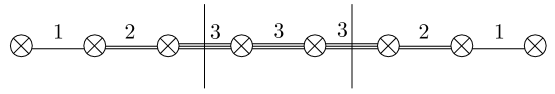
Figure 3: The NS5-D6-D8 configuration corresponding to the $\mathrm{[I_{5-3}]}$ model: circles with a cross represent NS5 branes, the horizontal lines are the D6’s and the vertical line are D8 branes.

3.2.2 $[\mathrm{I}_{n-p-q}]$ model

We now discuss a generalization of the previous model that includes a perturbative monodromy for the Wilson line $\beta$. This is the $[\mathrm{I}_{n-p-q}]$ model in the NU list and it is described by the following fibration:

$$y^{2}=(x^{2}+t^{n})\left[(x-1)^{2}+t^{m}\right]\left[(x-2)^{2}+t^{q}\right]\,,$$ (3.30)

which has the monodromy:

$$\tau\rightarrow\tau+m+q\,,\quad\rho\rightarrow\rho+n+q\,,\quad\beta\rightarrow\beta-q\,.$$ (3.31)

By proceeding as in the previous section, we obtain the following theory from the resolution of the $u=t=0$ intersection:

		$\mathfrak{su}(2)$	$\mathfrak{su}(4)$		$\widehat{\mathfrak{su}(2q)}$	$\mathfrak{su}(2q+1)$		$\widehat{\mathfrak{su}(k)}$	$\mathfrak{su}(k)^{\oplus m}$	$\widehat{\mathfrak{su}(k)}$	$\mathfrak{su}(k-1)$		$\mathfrak{su}(2)$
1	2	2	2	$\cdots$	2	2	$\cdots$	2	$(2)\times m$	2	2	$\cdots$	2	2

where we defined

$$k=p+q\,,\quad m=n-p-1\,,$$ (3.32)

and we assumed for simplicity that $n>p>q$. In fact, one can check that the result is completely symmetric under permutations of $(n,p,q)$. The hat indicates intersection with the residual discriminant and corresponds to an extra fundamental hypermultiplet. Note that there are a total of $(n+p+q)$ nodes in the quiver.

This type of quiver also appears in IIA brane models with intersecting NS5, D6 and D8 branes, as we discussed above, and this is again useful to understand the jumps in the rank of the gauge groups from the presence of D8 branes. We show in figure 4 the brane model giving the non-perturbative algebra of the model with $n=8,\,p=6\,,q=4$.

We refer to [16], section 5.1, for a more detailed discussion on the relation between the IIA models and the F-theory geometry. In particular, it is interesting to note that in a IIA model with multiple D8 branes along a “staircase”, one can bring all the D8 branes on one side by Hanany-Witten moves, and there are different number of D6 branes ending on them. After backreaction this gives “fuzzy funnels” (related to the shells of polarized D8 branes in the solutions of [49]) which were related in [16] to T-branes in the IIB frame. It would be interesting to understand more directly the relation of this T-brane data with the $\beta$-monodromies present in the heterotic context.

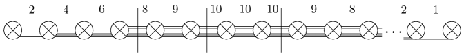
Figure 4: The NS5-D6-D8 configuration corresponding to the $[\mathrm{I}_{8-6-4}]$ model. We now have an additional D8 on the right hand side, which causes additional jumps in the rank of gauge groups.

4 Non-geometric models and duality web

We have seen that the explicit formulation of heterotic/F-theory duality in terms of the map between genus-two and K3 fibrations reproduces the expectation from the moduli monodromies in a number of situations where the heterotic side had a clear geometric interpretation, at least in some duality frame.

In this section we investigate heterotic models with monodromies which are non-geometric in all T-duality frames. This is the most interesting situation, since a priori it is not clear if such degenerations are allowed, and even basic quantities such as the charge of the corresponding “exotic” branes are not obviously available since we cannot go to a geometric frame, measure the charge, and dualize back.

One class of non-geometric models is obtained by combining Dehn twists of the two genus-one components of the genus-two fiber in order to have monodromies for $\tau$ and $\rho$ that remain non-geometric even after the exchange of $\tau$ and $\rho$. A simple example in the absence of Wilson lines is a double elliptic T-fold with monodromy $\tau\to-1/\tau\,,\rho\to-1/\rho$. We will find that all these models admit a dual smooth resolution, and moreover the resulting low energy physics is the same as the one describing the geometric models studied in the previous section. We believe that this result can be used as a non-trivial test of any direct description of non-geometric solutions, for example by using a T-duality covariant formalism such as double field theory [50, 51, 52]. We will shortly analyze in details the $\mathrm{[III-III]}$ model which is an interesting example of this class.

In sections 5 we will consider models whose monodromies involve Dehn twists along the cycle $\gamma$ that links the cycles of the homology basis (see figure 1), thus including a non-geometric mixing of the $\tau$ and $\rho$ moduli. As we will explain in detail, only few of these models admit a dual Calabi-Yau resolution, and for them we again derive the low energy description from the F-theory side.

4.1 Double elliptic T-fold: $\mathrm{[III-III]}$ model

As an example of a non-geometric degeneration we take the Namikawa-Ueno $\mathrm{[III-III]}$ singularity. This model has monodromy:

$$\tau\rightarrow\frac{\rho}{\beta^{2}-\rho\tau}\,,\quad\rho\rightarrow\frac{\tau}{\beta^{2}-\rho\tau}\,,\quad\beta\rightarrow-\frac{\beta}{\beta^{2}-\rho\tau}\,.$$ (4.1)

We see that when $\beta=0$ we obtain a “double elliptic” fibration on an $S^{1}$ that encircles the heterotic degeneration, with monodromy $\tau\to-1/\tau\,,\rho\to-1/\rho$. Models with such twists have been discussed in the past from different points of view (see for example [53, 54, 55, 31]). The equation for the hyperelliptic curve for such a singularity is:

$$y^{2}=x(x-1)(x^{2}+t)\left[(x-1)^{2}+t\right]\,.$$ (4.2)

Like for the resolutions in the previous section, we calculate the Siegel modular forms for this hyperelliptic fiber by using the map (2.9) and the explicit expressions for the Igusa-Clebsch invariants, and we plug them into equation (2.1). We find that $f$ and $g$ for this Weierstraß equation, look as follows:

$$f =-12t^{2}u^{3}v^{4}\big{(}41472t^{10}v+186624t^{9}v+334368t^{8}v+300672t^{7}v+139968t^{6}v$$

$$\quad+31104t^{5}v+16t^{4}u+2592t^{4}v+36t^{3}u+57t^{2}u+30tu+9u\big{)}\,,$$ (4.3)

$$g =u^{5}v^{5}\big{(}-3981312t^{15}v^{2}-8957952t^{14}v^{2}+11197440t^{13}v^{2}+57542400t^{12}v^{2}+78941952t^{11}v^{2}$$

$$\quad+54914112t^{10}v^{2}-1024t^{9}uv+21959424t^{9}v^{2}-3456t^{8}uv+5318784t^{8}v^{2}-288t^{7}uv$$

$$\quad+746496t^{7}v^{2}+9648t^{6}uv+46656t^{6}v^{2}+8640t^{5}uv+2160t^{4}uv+u^{2}\big{)}\,.$$ (4.4)

We are again interested in the enhancements from the intersection of the residual discriminant with the $E_{7}$ curve at $t=0$. The terms relevant for this analysis are

$$y^{2}=x^{3}+\left[t^{6}u^{3}+t^{2}u^{4}\right]x+t^{4}u^{6}+t^{6}u^{5}+u^{7}\,,$$ (4.5)

with a discriminant

$$\Delta=-u^{9}\left(4t^{18}+12t^{14}u+27t^{12}u+66t^{10}u^{2}+58t^{6}u^{3}+27t^{8}u^{3}+54t^{4}u^{4}+27u^{5}\right)$$ (4.6)

We see that at $u=t=0$ vanishing orders of $f$, $g$ and $\Delta$ increase to $(6,7,14)$. To resolve this singularity we proceed as in (3.7), introducing now six divisors $e_{i}$.

As a next step, we want to analyze the singularities that arise at the new exceptional curves to see what kind of gauge groups and matter we obtain. From the vanishing orders of $f$, $g$ and $\Delta$ along this curves we get the chain of $1\,2\,\,2\,2\,2\,2$ curves:

$$\mathrm{[III^{\ast}]-I_{0}-II-IV-I_{0}^{\ast}-IV-II}\,.$$ (4.7)

In order to identify the gauge groups, we look at the conditions in table 2. The analysis of the monodromy covers proceeds much as in the previous cases. We see that the $\mathrm{I_{0}^{*}}$ cover does not factorize, as we expect in the case that the curve is intersected by a curve with type $\mathrm{IV}$ singularity [56]. Hence we obtain a $\mathfrak{g}_{2}$ gauge algebra. For the type $\mathrm{IV}$ fibers we find $\mathfrak{sp}(1)$ because both curves have adjacent $\mathrm{I_{0}^{*}}$ and type $\mathrm{II}$ singularities [15]. The remaining divisors do not lead to a contribution to the gauge algebra and we thus find the following non-perturbative enhancement:

122222.fragments 122222\begin{tabular}[]{|cccccc|}\hline\cr&&$\mathfrak{sp}(1)$&$\mathfrak{g}_{2}$&$\mathfrak{sp}(1)$&\\ 1&2&2&2&2&2\\ \hline\cr\end{tabular}\,.

sp(1)g2sp(1)sp(1)g2sp(1) (4.8)

The matter spectrum for the gauge symmetries can now be deduced from anomaly cancellation or by studying the monodromy covers in more detail. From anomaly cancellation one obtains for $(-2)$-curves that we need four fundamentals for an $\mathfrak{su}(2)$ and four $\mathbf{7}$’s for a $\mathfrak{g}_{2}$. These states are partitioned into localized and non-local matter. Localized matter arises at the intersections of the curves whereas non-local matter, besides the adjoint, appears in the case of monodromies on the Kodaira fiber. Therefore, we obtain

$$e_{1}\cap e_{2}:\,\tfrac{1}{2}(\mathbf{1},\mathbf{2})\,,\quad e_{2}\cap e_{3}:\,\tfrac{1}{2}(\mathbf{2},\mathbf{7})\,,\quad e_{3}:2\times\mathbf{7}\textmd{ (non-loc.)}\,,\quad e_{3}\cap e_{4}:\,\tfrac{1}{2}(\mathbf{7},\mathbf{2})\,,\quad e_{4}\cap e_{5}:\,\tfrac{1}{2}(\mathbf{2},\mathbf{1})\,.$$ (4.9)

As a check of the amount of non-local matter, we calculate the genus of the monodromy cover over $e_{3}$ (for $e_{2}$ and $e_{4}$ checks can be done in a similar fashion), which is given by:

$$\psi^{3}+2^{2}3^{3}e_{2}^{2}\,e_{4}^{2}\,(2^{4}3^{3}\,e_{2}^{2}+e_{4}^{2}-\psi)=0\,,$$ (4.10)

where $e_{2}$ and $e_{4}$ are the homogeneous coordinates of the rational line $e_{3}=0$. From (4.10) we see that the cover is singular at $\psi=e_{2}=0$ and $\psi=e_{4}=0$. Resolving these two singularities, we find that the genus of the cover is two which agrees with the two non-local $\mathbf{7}$-states that we needed for anomaly cancellation. We summarise this resolution in figure 5.

Figure 5: Pictorial summary of the gauge algebra and matter content that arise from the resolution of the dual model of a $\mathrm{[III-III]}$ singularity.

At this point, we can check that what we obtained is precisely the same resolution as the one obtained from the NU model $\mathrm{[I_{0}^{\ast}-I_{0}]}$ in (A.21), giving the theory of six pointlike instantons on a $D_{4}$ singularity. At first sight, this seems very surprising, since we started from two different elements of the NU list, whose monodromies are not conjugate to each other and there seems to be no duality that brings a degeneration of type $\mathrm{[III-III]}$ to a geometric frame. However, this is in line with the fact that no new F-theory models are needed to understand the class of non-geometric heterotic models where $\tau$ and $\rho$ degenerations do not collide [3]. In the following we will generalize this observation to obtain a list of all the models described by the same six-dimensional low energy theory. However, before we detour to describe a global embedding of the local $\mathrm{[III-III]}$ model.

4.2 A global model

In this section we address the question of global hyperelliptic fibrations. The idea is to first start with the generic situation and continue by tuning the coefficients $c_{i}$ in (2.7) to obtain different kinds of singularities. In practice we have to choose the parameters $\gamma_{ij}$ in (2.21). We will consider an example that features a $\mathrm{[III-III]}$ singularity, discussed in section 4.1, at the origin.

The concrete hyperelliptic curve can be obtained by taking the local equation (4.2) and extending the prefactors of $x^{i}$ to sections of the anti-canonical bundle of $\mathbb{P}^{1}$, cf. section 2.3, which reduce near $t=0$ to the ones from (4.2),

$$\begin{split}y^{2}=&x^{6}\left(\delta_{62}t^{2}+\delta_{61}t+1\right)+x^{5}\left(\delta_{52}t^{2}+\delta_{51}t-3\right)+x^{4}\left(\delta_{4}t^{2}+2t+3\right)+\\ &+x^{3}\left(\delta_{3}t^{2}-4t-1\right)+\left(t^{2}+3t\right)x^{2}+\left(-t^{2}-t\right)x\,.\end{split}$$ (4.11)

Here $t$ is the affine coordinate on the ${\mathbb{P}}^{1}$ base. When we calculate from this sextic the vanishing orders of the Siegel modular forms at $t=0$, we find

$$\mu(\psi_{4})=2\,,\quad\mu(\psi_{6})=3\,,\quad\mu(\chi_{10})=5\,,\quad\mu(\chi_{12})=5\,.$$ (4.12)

However, these are the vanishing orders of the $\mathrm{[II-III]}$ singularity as one can see from Table 5. Therefore, we have to look at the coefficients of the $t^{3}$, $t^{5}$, $t^{5}$ terms in $\psi_{6}$, $\chi_{10}$, $\chi_{12}$, respectively. All of them are proportional to $\delta_{61}+\delta_{51}$. Hence, we set $\delta_{51}\equiv-\delta_{61}$ in (4.11) to obtain indeed a $\mathrm{[III-III]}$ at $t=0$.

The discriminant of this sextic is found to be

$$I_{10}=\frac{1}{2\cdot 3^{5}}\,\chi_{10}=t^{6}(t+1)^{2}P_{12}(t)\,,$$ (4.13)

where $P_{12}(t)$ is a polynomial of degree 12 with simple roots, say $r_{\ell}$, $\ell=1,\ldots,12$. Thus, the fiber degenerates at $t=0$, $t=-1$, and the twelve roots $r_{\ell}$. There is no singularity at $\infty$. To analyze the type of singularities—besides the one at $t=0$ which we know already—we compute the vanishing orders of the Siegel modular forms at the remaining singularities:

$$\begin{split}t=-1:&\quad\mu(\psi_{4})=0\,,\quad\mu(\psi_{6})=0\,,\quad\mu(\chi_{10})=2\,,\quad\mu(\chi_{12})=2\,,\\ t=r_{\ell}:&\quad\mu(\psi_{4})=0\,,\quad\mu(\psi_{6})=0\,,\quad\mu(\chi_{10})=1\,,\quad\mu(\chi_{12})=1\,.\end{split}$$ (4.14)

From the tables of section 6.2, we find that the singularity at $t=-1$ is of type $\mathrm{[I_{2-0-0}]}$ and the singularities at $t=r_{\ell}$ are of type $\mathrm{[I_{1-0-0}]}$.

Let us now examine the global model from the F-theory perspective. To analyze the singularities on the F-theory side we first determine the discriminant of the elliptic fibration (2.1)

$$\Delta=u^{9}\left[4(au+c)^{3}+27u(u^{2}+bu+d)^{2}\right]=u^{9}P_{5,60}(u,t)\,,$$ (4.15)

where $P_{5,60}(u,t)$ is the polynomial of degree 5 and 60 in the affine coordinate $u$ and $t$ of $\mathbb{F}_{12}$, respectively, read off from the equality. The discriminant clearly exhibits the $E_{7}$ and $E_{8}$ singular fibers at $u=0$ and $u=\infty$, respectively, i.e. along the two sections of the Hirzebruch surface. But now we are more interested in locating additional singular loci. Looking at $P_{5,60}(u,t)$ we find that it does not factorize any further, i.e. $P_{5,60}(u,t)=0$ defines an $\mathrm{I_{1}}$ locus. This $\mathrm{I_{1}}$ curve intersects the section $u=0$. At the intersection points of $\mathrm{I_{1}}$ and $\mathrm{III^{*}}$ where also $c$ and $d$ vanish, we obtain singularities of non-minimal type (or non-Kodaira type). Note that these are exactly the loci where also the genus-two curve degenerates. The resolution of these singularities (on the F-theory side) were already analyzed in Section 3.2.1 and 4.1. Besides these points there are no other co-dimension two singularities which render the Calabi-Yau threefold singular, although there might be other points where the K3, or the elliptic fiber, degenerates. In particular, we find that the points associated with the enhancement to $SU(2)$ of the heterotic at self-dual points, giving $SU(2)$ singularities on the K3 fiber, do not lead to singularities in the total space of the K3 fibration.

4.3 Dualities

We have seen that the resolution of the dual $\mathrm{[III-III]}$ model gives the same six-dimensional theory as $\mathrm{[I_{0}-I_{0}^{\ast}]}$, namely the theory of six pointlike instantons on a $D_{4}$ singularity. In fact, this is not an isolated coincidence, as we argue below.

We first note that the above mentioned duality might be understood from the monodromy factorization of the two models as we now explain. From table 1, and our discussion in section 2.2, it follows that the monodromy of the $\mathrm{[III-III]}$ model can be written in terms of products of Dehn twists as $B_{1}A_{1}B_{1}B_{2}A_{2}B_{2}$. Recall that $A_{i}$ and $B_{i}$ are respectively twists around the $a_{i}$ and $b_{i}$ cycles shown in figure 1. We can get to the monodromy of the $\mathrm{[I_{0}-I_{0}^{\ast}]}$ model by applying the following moves:

$$\begin{split}\mathrm{[III-III]}&=B_{1}A_{1}B_{1}B_{2}A_{2}B_{2}\\ &=B_{1}A_{1}B_{1}B_{1}A_{1}B_{1}\qquad(\rho\rightarrow\tau)\\ &=B_{1}A_{1}B_{1}A_{1}B_{1}A_{1}\qquad(\text{braid})\\ &=(B_{1}A_{1})^{3}=\mathrm{[I_{0}-I_{0}^{\ast}]}\,.\end{split}$$ (4.16)

The last move follows from braid relations that define the generators of the mapping class group (see for example [31]), and it is the analogous of a collision of two Kodaira fibers of type $\mathrm{III}$ in F-theory. The first move replaces locally the $\rho$ fibration with a fibration in $\tau$. We can check that this move is allowed in the case of the elliptic models from the direct inspection of the duality map for the $E_{8}\times E_{8}$ case, which is considerably simpler and it is shown in appendix B.

This simple argument also predicts that the $\mathrm{[I_{0}-I_{0}^{\ast}]}$ model is equivalent to the $\mathrm{[IV-II]}$ model, described by the fibration:

$$y^{2}=(t+x^{3})\left[t^{2}+(x-1)^{3}\right]\,,$$ (4.17)

and corresponding to a monodromy $B_{1}A_{1}B_{1}A_{1}B_{2}A_{2}$. By constructing the dual F-theory model and resolving it, we indeed find the same six-dimensional theory.

$\mu(I_{10})$	dual models
2	$\mathrm{[I_{0}-II]}_{0112}$
3	$\mathrm{[I_{0}-III]}_{0113}$
4	$\mathrm{[I_{0}-IV]}_{0224}\,,\,\mathrm{[II-II]}_{0224}$
5	$[\mathrm{IV}-\mathrm{I}_{1}]_{0325}\,,\,\mathrm{[II-III]}_{0225}$
6	$\mathrm{[I_{0}-I_{0}^{\ast}]}_{0226}\,,\,\mathrm{[III-III]}_{0226}\,,\,\mathrm{[IV-II]}_{0336}$
7	$[\mathrm{I}_{0}^{\ast}-\mathrm{I}_{1}]_{0227}\,,\,\mathrm{[IV-III]}_{0337}$
8	$\mathrm{[I_{0}-IV^{\ast}]}_{0448}\,,\mathrm{[IV-IV]}_{0448}\,,\,\mathrm{[I_{0}^{\ast}-II]}_{0338}$
9	$\mathrm{[I_{0}-III^{\ast}]}_{0339}\,,\,\mathrm{[I_{0}^{\ast}-III]}_{0339}$
10	$\mathrm{[I_{0}-II^{\ast}]}_{0\,5\,5\,10}\,,\,\mathrm{[IV^{\ast}-II]}_{0\,5\,5\,10}\,,\,\mathrm{[I_{0}^{\ast}-IV]}_{0\,4\,4\,10}$
11	$\mathrm{[II-III^{\ast}]}_{0\,4\,4\,11}\,,\,\mathrm{[IV^{\ast}-III]}_{0\,5\,5\,11}$

Table 3: Dual models: the NU degenerations in the same row give rise to the same SCFTs after resolution of the dual F-theory model. We indicate as a subscript the vanishing orders of the Igusa-Clebsch invariants $I_{2}\,,I_{4}\,,I_{6}\,,I_{10}$.

As a rule, we can find dual models if the sum of the orders of the discriminant for their two Kodaira components, or equivalently the order of the Igusa-Clebsch invariant $I_{10}$, is the same. In table 3 we display all the models of this type that have the same order. We indicate as a subscript the order of vanishing of all the Igusa-Clebsch invariants, listed in appendix D. In section 6 we show that models with higher $\mu(I_{10})$ do not admit dual smooth Calabi-Yau resolutions. For all the models in table 3 we explicitly performed the F-theory resolution and verified that for all the degenerations in a row the same theory arises.

We thus see that almost all non-geometric models of type 2 in the NU list are described by the theory of pointlike instantons on ADE singularities. It would be interesting to understand better this fact directly from the heterotic side, beyond the simple argument given above. The precise set of dualities that we are finding should also be an interesting test of T-duality covariant formalisms, such as double field theory [50, 51, 52], in which one might hope to describe non-geometric backgrounds. Presumably, these dualities can be clarified by understanding the non-geometric analog of the Bianchi identity 3.1.

We also stress that our findings imply the existence of local degenerations with monodromies which are non-geometric in all T-duality frames, thus enlarging the examples of “exotic” branes recently studied for example in [29, 30], and provide a dual description of the T-fects constructed in [31].

5 Other models

In the previous sections we explored parabolic models in the NU classifications that had a clear geometric interpretation, and elliptic models of type $\mathrm{[K_{1}-K_{2}]}$, both geometric and non-geometric, whose dual resolutions can be understood in terms of the theory of pointlike instantons on ADE singularities. In this section we consider examples from the remaining NU models, in particular we explore models whose monodromies involve a twist along the cycle $\gamma$ in figure 1. As we will show in the next section, the duals of many models of this kind cannot be resolved, so we restrict ourselves to the examples that admit a smooth dual Calabi-Yau model.

5.1 Non-geometric degenerations with moduli mixing

A list of genus-two degenerations with monodromy that mixes the moduli is provided by the elliptic type 1 models in the NU classification (see appendix D). Despite the fact that the corresponding heterotic models lack a geometric interpretation, the dual F-theory resolutions are similar to the ones encountered in the previous sections. For each example we again determine the non-perturbative gauge algebras. We refer to section 6 for a detailed analysis of all the type 1 models, which shows that the models listed here are the only ones admitting a smooth dual.

$\mathrm{[V]}$ model

From the NU list we take the local model:

$$y^{2}=x^{6}+t\,,$$ (5.1)

whose $Sp(4,\mathbb{Z})$ monodromy is

$$M_{\mathrm{[V]}}=\begin{pmatrix}0&0&1&0\\ 0&0&1&1\\ -1&1&0&0\\ 0&-1&0&0\end{pmatrix}\,,$$ (5.2)

which acts on the moduli matrix $\eqref{omatrix}$ as

$$\tau\rightarrow\frac{\rho}{\beta^{2}-\rho\tau}\,,\qquad\rho\rightarrow\frac{\rho+\tau-2\beta}{\beta^{2}-\rho\tau}\,,\qquad\beta\rightarrow\frac{\rho-\beta}{\beta^{2}-\rho\tau}\,.$$ (5.3)

This is an elliptic monodromy of order six, and up to global conjugation it can be decomposed into the following product of the $Sp(4,\mathbb{Z})$ generators given in (2.12):

$$M_{\mathrm{[V]}}=A_{1}B_{1}\Gamma B_{2}A_{2}\,.$$ (5.4)

By computing the Igusa-Clebsch invariants we find the following dual K3 fibration:

$$y^{2}=x^{3}+972t^{2}u^{3}v^{4}(-5u+2^{7}3^{6}t^{3}v)x+u^{5}v^{5}(u^{2}-2^{4}3^{6}5t^{3}uv+2^{11}3^{12}5t^{6}v^{2})\,,$$ (5.5)

with discriminant:

$$\Delta=-27u^{9}v^{10}\left(2^{5}3^{6}t^{3}v+u\right)^{3}\left(2^{7}3^{6}t^{3}v-u\right)^{2}\,.$$ (5.6)

By resolving the intersection $u=t=0$ we get a chain:

$$\mathrm{[III^{\ast}]-I_{0}-III-I_{0}^{\ast}-IV-II}\,.$$ (5.7)

The vanishing orders of $f$ and $g$ at each divisor indicate the following gauge algebras:

12222.fragments 12222\begin{tabular}[]{|ccccc|}\hline\cr&$\mathfrak{su}(2)$&$\mathfrak{g}_{2}$&$\mathfrak{sp}(1)$&\\ 1&2&2&2&2\\ \hline\cr\end{tabular}\,.

su(2)g2sp(1)su(2)g2sp(1) (5.8)

The matter content is $\frac{1}{2}(\mathbf{2},\mathbf{1},\mathbf{1})\oplus\frac{1}{2}(\mathbf{2},\mathbf{7},\mathbf{1})\oplus 2(\mathbf{1},\mathbf{7},\mathbf{1})\oplus\frac{1}{2}(\mathbf{1},\mathbf{7},\mathbf{2})\oplus\frac{1}{2}(\mathbf{1},\mathbf{1},\mathbf{2})$, in agreement with anomaly cancellation [18, 15].

We find the same result for another model that admits a dual smooth fibration, the $\mathrm{[VII]}$ model described by $y^{2}=x(x^{4}+t)$ and monodromy

$$M_{\mathrm{[VII]}}=\begin{pmatrix}0&1&1&0\\ 1&-1&0&1\\ -1&1&1&0\\ 0&-1&0&0\end{pmatrix}\,.$$ (5.9)

$\mathrm{[VIII-1]}$ model

This example is defined by:

$$y^{2}=x^{5}+t\,,$$ (5.10)

with monodromy matrix

$$M_{\mathrm{[VIII-I]}}=\begin{pmatrix}0&1&1&0\\ 1&0&0&1\\ -1&1&1&0\\ 0&-1&0&0\end{pmatrix}\,.$$ (5.11)

The action on the moduli is found to be

$$\tau\rightarrow\frac{\rho}{\beta^{2}+\rho-\rho\tau}\,,\qquad\rho\rightarrow\frac{\tau(\rho+1)-(\beta+1)^{2}}{\beta^{2}+\rho-\rho\tau}\,,\qquad\beta\rightarrow\frac{\rho\tau-\beta(\beta+1)}{\beta^{2}+\rho-\rho\tau}\,.$$ (5.12)

In this model only the Igusa-Clebsch invariant $I_{10}$ does not vanish identically. The dual F-theory elliptic fibration is then:

$$y^{2}=x^{3}-2^{3}3^{5}5^{5}t^{4}u^{3}v^{5}x+u^{7}v^{5}\,,\quad\Delta=-27u^{9}v^{10}\left(u^{5}-2^{11}3^{12}5^{15}t^{12}v^{5}\right)\,,$$ (5.13)

leading to a simple chain

$$\mathrm{[III^{\ast}]-I_{0}-III-IV-II}$$ (5.14)

with gauge algebras:

1222.fragments 1222\begin{tabular}[]{|cccc|}\hline\cr&$\mathfrak{su}(2)$&$\mathfrak{sp}(1)$&\\ 1&2&2&2\\ \hline\cr\end{tabular}\,.

su(2)sp(1)su(2)sp(1) (5.15)

The matter comprises a bifundamental plus one additional $\mathbf{2}$ for each factor.

$\mathrm{[IX-1]}$ model

As a last example we consider the NU model:

$$y^{2}=x^{5}+t^{2}\,,$$ (5.16)

with monodromy matrix

$$M_{\mathrm{[IX-1]}}=\begin{pmatrix}0&1&1&1\\ 0&0&1&0\\ 0&0&0&1\\ -1&0&0&-1\end{pmatrix}\,,$$ (5.17)

acting on the moduli as:

$$\tau\rightarrow 1+\rho-\frac{(1+\beta)^{2}}{\tau}\,,\qquad\rho\rightarrow-\frac{1}{\tau}\,,\qquad\beta\rightarrow-\frac{\beta+1}{\tau}\,.$$ (5.18)

In this case it also happens that $a=b=d=0$ and the dual elliptic fibration is

$$y^{2}=x^{3}-2^{3}3^{5}5^{5}t^{8}u^{3}v^{5}x+u^{7}v^{5}\,,\quad\Delta=-27u^{9}v^{10}\left(u^{5}-2^{11}3^{12}5^{15}t^{24}v^{5}\right)\,.$$ (5.19)

Resolving $u=t=0$ now requires a total of 16 blowups and gives the chain:

$$\mathrm{[III^{\ast}]-I_{0}-III-I_{0}^{\ast}-III-I_{0}-III^{\ast}-I_{0}-II-IV-I_{0}^{\ast}-II-IV^{\ast}-II-I_{0}^{\ast}-IV-II}\,.$$ (5.20)

The study of monodromy covers, cf. table 2 leads to the following non-perturbative gauge algebras:

1232181223151322.fragments 1232181223151322\begin{tabular}[]{|cccccccccccccccc|}\hline\cr&$\mathfrak{su}(2)$&$\mathfrak{so}(7)$&$\mathfrak{su}(2)$&&$\mathfrak{e}_{7}$&&&$\mathfrak{sp}(1)$&$\mathfrak{g}_{2}$&&$\mathfrak{f}_{4}$&&$\mathfrak{g}_{2}$&$\mathfrak{sp}(1)$&\\ 1&2&3&2&1&8&1&2&2&3&1&5&1&3&2&2\\ \hline\cr\end{tabular}\,.

su(2)so(7)su(2)e7sp(1)g2f4g2sp(1)su(2)so(7)su(2)e7sp(1)g2f4g2sp(1) (5.21)

The only matter representations are $\frac{1}{2}(\mathbf{2},\mathbf{8},\mathbf{1})\oplus\frac{1}{2}(\mathbf{1},\mathbf{8},\mathbf{2})$, for $\mathfrak{su}(2)\oplus\mathfrak{so}(7)\oplus\mathfrak{su}(2)$.

As we already mentioned, in the type 1 NU elliptic models there are no other heterotic degenerations that admit a dual Calabi-Yau resolution.

5.2 Parabolic models of type 3

In the parabolic type 3 class of the NU list we find additional models that admit smooth F-theory duals. Below we present the resolution of several examples.

$[\mathrm{II}_{n-0}]$ model

The model $[\mathrm{II}_{n-0}]$ is described by the local equation:

$$y^{2}=(x^{4}+\alpha tx^{2}+t^{2})\left[(x-1)^{2}+t^{n-1}\right]\,,$$ (5.22)

and has monodromy

$$\tau\rightarrow\tau\,,\quad\rho\rightarrow\rho+\tau-2\beta+n\,.\quad\beta\rightarrow\tau-\beta\,.$$ (5.23)

The intersection of $\{t=0\}$ with the $E_{7}$ curve in the dual F-theory model is described by

$$y^{2} =x^{3}+\left[t^{5+n}u^{3}+t^{2}u^{4}\right]x+t^{6+n}u^{5}+t^{3}u^{6}+u^{7}\,,$$ (5.24)

$$\Delta =-u^{9}\left(54u^{3}t^{n+6}+66u^{2}t^{n+9}+39ut^{2n+12}+4t^{3n+15}+31t^{6}u^{3}+54t^{3}u^{4}+27u^{5}\right)\,.$$

The resolution produces a plateau of $\mathrm{I_{0}^{\ast}}$ Kodaira fibers, which after further resolution gives the chain:

$$\mathfrak{su}(2)$$

1 2 3 1 4 1 4 1 3 2 2

(5.25)

Chains of type $1\,4\cdots 1\,4$, with $\mathfrak{so}(8)$ singularities, are described in detail in [56]. The resolution is similar to that in the $[\mathrm{I}_{0}^{\ast}-\mathrm{I}_{n}]$ model (see appendix A), but in this case the plateau $14\cdots 41$ is connected with the $E_{7}$ in a different way. There is a chain $123$ instead of $1223$, and there is a $\mathfrak{su}(2)\times\mathfrak{so}(7)$ with matter $\frac{1}{2}({\mathbf{2}},{\mathbf{8}})\oplus({\mathbf{1}},{\mathbf{8}})$, as expected from anomaly cancellation. It would be interesting to understand better the heterotic interpretation of this model.

$[\mathrm{IV}-\mathrm{I}_{n}^{*}]$ model

The defining local equation is given by:

$$y^{2}=(t+x)(x^{2}+t^{n+2})\left[(x-1)^{3}+t^{2}\right]\,.$$ (5.26)

The monodromy action turns out to be:

$$\tau\rightarrow-\frac{1}{1+\tau}\,,\quad\rho\rightarrow\rho+n-\frac{\beta^{2}}{1+\tau}\,,\quad\beta\rightarrow\frac{\beta}{1+\tau}\,.$$ (5.27)

Here, and in the remaining examples of this section, we will skip presenting the data of the dual K3 on the F-theory side. To resolve we proceed as explained before. We obtain a resolution precisely equal to that of $[\mathrm{II^{*}}-\mathrm{I}_{n}]$, corresponding to $(10+n)$ pointlike instantons on an $E_{8}$ singularity, discussed in sections 3.1 and 3.1.1. We find that other examples of type $[\mathrm{K}-\mathrm{I}_{n}^{*}]$ do match models, analyzed in appendix A, associated to pointlike instantons on $E_{7}$, $E_{6}$ and $D_{4}$ singularities. Indeed, the resolutions of $[\mathrm{III}-\mathrm{I}_{n}^{*}]$ and $[\mathrm{III^{*}}-\mathrm{I}_{n}]$, $[\mathrm{II}-\mathrm{I}_{n}^{*}]$ and $[\mathrm{IV^{*}}-\mathrm{I}_{n}]$, as well as $[\mathrm{I}_{0}-\mathrm{I}_{n}^{*}]$ and $[\mathrm{I}_{n}-\mathrm{I}_{0}^{*}]$, do coincide.

$[\mathrm{IV^{*}}-\mathrm{II}_{n}]$ model

According to the NU list the local singularity is described by:

$$y^{2}=x(x^{3}+t^{2})\left[(x-1)^{2}+t^{n-1}\right]\,,$$ (5.28)

for $n\geq 1$. The monodromy action translates into:

$$\tau\rightarrow-\frac{1+\tau}{\tau}\,,\quad\rho\rightarrow\rho+n-\frac{\beta^{2}}{\tau}\,,\quad\beta\rightarrow-1+\frac{\beta}{\tau}\,.$$ (5.29)

The resolution has the structure:

12321​ 6131⊗n​ 51322.fragments 12321superscriptfragments 6131tensor-productabsent𝑛fragments 51322\begin{tabular}[]{|ccccc|}\hline\cr&$\mathfrak{su}(2)$&$\mathfrak{so}(7)$&$\mathfrak{su}(2)$&\\ 1&2&3&2&1\\ \hline\cr\end{tabular}\,\begin{tabular}[]{|cccc|}\hline\cr$\mathfrak{e}_{6}$&&$\mathfrak{su}(3)$&\\ 6&1&3&1\\ \hline\cr\end{tabular}^{\,\otimes n}\,\begin{tabular}[]{|ccccc|}\hline\cr$\mathfrak{f}_{4}$&&$\mathfrak{g}_{2}$&$\mathfrak{sp}(1)$&\\ 5&1&3&2&2\\ \hline\cr\end{tabular}\,.

su(2)so(7)su(2)e6su(3)f4g2sp(1)su(2)so(7)su(2)e6su(3)f4g2sp(1) (5.30)

The second and third block in the above pattern appear in the resolution of the $[\mathrm{I}_{n+1}-\mathrm{IV}^{*}]$ model, cf. (A.20), associated to $k=n+9$ pointlike instantons on a $E_{6}$ singularity. It can also be checked that the resolution of $[\mathrm{II}-\mathrm{II}^{*}_{n}]$ gives the same result (5.30).

$[\mathrm{III}-\mathrm{II}_{n}^{*}]$ model

From the NU list we read the singularity type:

$$y^{2}=(x^{4}+t)(x^{2}+t^{n+1})\,.$$ (5.31)

The characteristic monodromy is given by:

$$\tau\rightarrow-\frac{1}{\tau}\,,\quad\rho\rightarrow\rho+n-\frac{\beta^{2}}{\tau}\,,\quad\beta\rightarrow 1+\frac{\beta}{\tau}\,.$$ (5.32)

Resolving yields:

12321 712321×\displaystyle\begin{tabular}[]{|ccccc|}\hline\cr&$\mathfrak{su}(2)$&$\mathfrak{so}(7)$&$\mathfrak{su}(2)$&\\ 1&2&3&2&1\\ \hline\cr\end{tabular}\,\begin{tabular}[]{|cccccc|}\hline\cr$\mathfrak{e}_{7}$&&$\mathfrak{su}(2)$&$\mathfrak{so}_{7}$&$\mathfrak{su}(2)$&\\ 7&1&2&3&2&1\\ \hline\cr\end{tabular}\,\times 812321⊕(n−1)× 8123151322.absentsuperscriptfragments 812321direct-sum𝑛1fragments 8123151322\displaystyle\times\begin{tabular}[]{|cccccc|}\hline\cr$\mathfrak{e}_{7}$&&$\mathfrak{su}(2)$&$\mathfrak{so}_{7}$&$\mathfrak{su}(2)$&\\ 8&1&2&3&2&1\\ \hline\cr\end{tabular}^{\,\oplus(n-1)}\times\hskip 5.69054pt\begin{tabular}[]{|cccccccccc|}\hline\cr$\mathfrak{e}_{7}$&&$\mathfrak{su}(2)$&$\mathfrak{g}_{2}$&&$\mathfrak{f}_{4}$&&$\mathfrak{g}_{2}$&$\mathfrak{sp}(1)$&\\ 8&1&2&3&1&5&1&3&2&2\\ \hline\cr\end{tabular}\,.

su(2)so(7)su(2)e7su(2)so7su(2) (5.37)

e7su(2)so7su(2)e7su(2)g2f4g2sp(1)e7su(2)so7su(2)e7su(2)g2f4g2sp(1) (5.42)

Except for the first block, this result resembles the resolution of the $[\mathrm{I}_{n+1}-\mathrm{III}^{*}]$ model, cf. (A.11), corresponding to $k=n+10$ pointlike instantons on an $E_{7}$ singularity. Matter includes representations $\frac{1}{2}(\mathbf{2},\mathbf{8},\mathbf{1})\oplus\frac{1}{2}(\mathbf{1},\mathbf{8},\mathbf{2})$ for each $\mathfrak{su}(2)\oplus\mathfrak{so}(7)\oplus\mathfrak{su}(2)$ block. In addition, we have verified that there is an extra half-fundamental for the $\mathfrak{e}_{7}$ with self-intersection $-7$, as required by anomaly cancellation. The same resolution (5.37) is obtained for $[\mathrm{III^{*}}-\mathrm{II}_{n}]$.

$[\mathrm{III}-\mathrm{II}_{n}]$ and $[\mathrm{IV}-\mathrm{II}_{n}]$ models

For these models we will only give the resolution for completeness. For $[\mathrm{III}-\mathrm{II}_{n}]$ we find

122⋯22.fragments 122⋯22\begin{tabular}[]{|cccccc|}\hline\cr&$\mathfrak{su}(2)_{1}$&$\mathfrak{su}(2)_{2}$&&$\mathfrak{su}(2)_{n+1}$&\\ 1&2&2&$\cdots$&2&2\\ \hline\cr\end{tabular}\,.

su(2)1su(2)2su(2)+n1su(2)1su(2)2su(2)+n1 (5.43)

Notice the similarity to the resolution of $[\mathrm{III}-\mathrm{I}_{n+1}]$ displayed in (A.33). For $[\mathrm{IV}-\mathrm{II}_{n}]$ we obtain

122⋯222.fragments 122⋯222\begin{tabular}[]{|ccccccc|}\hline\cr&$\mathfrak{su}(2)$&$\mathfrak{su}(3)_{1}$&&$\mathfrak{su}(3)_{n}$&$\mathfrak{sp}(1)$&\\ 1&2&2&$\cdots$&2&2&2\\ \hline\cr\end{tabular}\,.

su(2)su(3)1su(3)nsp(1)su(2)su(3)1su(3)nsp(1) (5.44)

This result is analogous to the resolution of $[\mathrm{IV}-\mathrm{I}_{n+1}]$ shown in (A.32).

5.3 Parabolic models of type 4

In this class we find 3 models that admit a resolution, the $[\mathrm{I}_{n-p-0}]$, already discussed in section 3.2.1, as well as $[\mathrm{II}_{n-p}]$ and $[\mathrm{I}_{n}-\mathrm{I}_{p}^{*}]$, which are addressed below.

$[\mathrm{II}_{n-p}]$ model

In the NU list we find two models that generalize $[\mathrm{II}_{n-0}]$, namely the $[\mathrm{II}_{n-p}]$ degenerations. Here we consider the one classified as type 4, with the following sextic:

$$y^{2}=(x^{2}+t)(x^{2}+t^{p+1})\left[(x-1)^{2}+t^{n-1}\right]\,,$$ (5.45)

and monodromy:

$$\tau\rightarrow\tau+p\,,\quad\rho\rightarrow\rho+n\,,\quad\beta\rightarrow-\beta-1\,.$$ (5.46)

The intersection $u=t=0$ in the dual F-theory model is given by the Weierstraß model:

$$y^{2}=x^{3} +\left[12(10368t^{5+n+p}+\cdots)u^{3}-12(t^{2}+\cdots)u^{4}\right]x$$ (5.47)

$$+497664(t^{6+n+p}+\cdots)u^{5}+16(t^{3}+\cdots)u^{6}+u^{7}\,.$$

Here we have written numerical factors in the leading terms in order to stress that in this case there will be non-generic cancellations in the discriminant $\Delta$. Computing $\Delta$ explicitly we can extract the data needed to perform the resolution. Proceeding as explained before, we find a chain $1231(414\cdots 14)1322$ supporting singularities $\mathrm{I}_{0}-\mathrm{III}-\mathrm{I}^{*}_{0}-\mathrm{I}_{1}-(\mathrm{I}^{*}_{1}-\cdots-\mathrm{I}^{*}_{1})-\mathrm{I}_{1}-\mathrm{I}^{*}_{0}-\mathrm{IV}-\mathrm{II}$. In the central block the $-1$ curves support $\mathfrak{sp}$ algebras whereas the $-4$ curves support $\mathfrak{so}$ ones. For example, for $n=p$, the full resolution takes the form:

14⋯141322.absentfragments 14⋯141322\displaystyle\times\begin{tabular}[]{|ccccccccc|}\hline\cr$\mathfrak{sp}(p-1)$&$\mathfrak{so}(2p+5)$&$\cdots$&$\mathfrak{sp}(1)$&$\mathfrak{so}(9)$&&$\mathfrak{g}_{2}$&$\mathfrak{sp}(1)$&\\ 1&4&$\cdots$&1&4&1&3&2&2\\ \hline\cr\end{tabular}\,.

$$\begin{tabular}[]{|cccccccccccc|}\hline\cr&$\mathfrak{su}(2)$&$\mathfrak{so}(7)$&&$\mathfrak{so}(9)$&$\mathfrak{sp}(1)$&$\mathfrak{so}(11)$&$\mathfrak{sp}(2)$&$\cdots$&$\mathfrak{so}(2p+5)$&$\mathfrak{sp}(p-1)$&$\mathfrak{so}(2p+7)$\\ 1&2&3&1&4&1&4&1&$\cdots$&4&1&4\\ \hline\cr\end{tabular}\times$$ (5.50)

sp(-p1)so(+2p5)⋯sp(1)so(9)g2sp(1)sp(-p1)so(+2p5)⋯sp(1)so(9)g2sp(1) (5.53)

The matter for $\mathfrak{sp}-\mathfrak{so}$, and viceversa, is $\frac{1}{2}(\bf{fund},\bf{fund})$. For $\mathfrak{so}(2p+7)$ there is an additional fundamental. In this way all gauge anomalies are canceled. The pattern is analogous to that obtained for $k=2p+6$ instantons on a $D_{p+4}$ singularity [18]. When $n>p$ the resolution is instead:

12314⋯141𝔰𝔬(2p+8)𝔰𝔭(p)41⊕(n−p−1)×\displaystyle\begin{tabular}[]{|ccccccccc|}\hline\cr&$\mathfrak{su}(2)$&$\mathfrak{so}(7)$&&$\mathfrak{so}(9)$&$\cdots$&$\mathfrak{sp}(p-1)$&$\mathfrak{so}(2p+7)$&$\mathfrak{sp}(p)$\\ 1&2&3&1&4&$\cdots$&1&4&1\\ \hline\cr\end{tabular}\,\begin{tabular}[]{|cc|}\hline\cr$\mathfrak{so}(2p+8)$&$\mathfrak{sp}(p)$\\ 4&1\\ \hline\cr\end{tabular}^{\,\oplus(n-p-1)}\times

su(2)so(7)so(9)⋯sp(-p1)so(+2p7)sp(p) (5.58)

$$\times\begin{tabular}[]{|cccccccccc|}\hline\cr$\mathfrak{so}(2p+7)$&$\mathfrak{sp}(p-1)$&$\mathfrak{so}(2p+5)$&$\cdots$&$\mathfrak{sp}(1)$&$\mathfrak{so}(9)$&&$\mathfrak{g}_{2}$&$\mathfrak{sp}(1)$&\\ 4&1&4&$\cdots$&1&4&1&3&2&2\\ \hline\cr\end{tabular}\,.$$ (5.61)

This result is similar to the resolution of $k>2p+6$ instantons on a $D_{p+4}$ singularity [18]. It can be checked that the matter content guarantees anomaly cancellation. For instance, for $n=4$, $p=3$, besides $\frac{1}{2}(\bf{fund},\bf{fund})$ for adjacent $\mathfrak{sp}-\mathfrak{so}$ and $\mathfrak{so}-\mathfrak{sp}$, there is an additional $\frac{1}{2}(\bf{1},\bf{fund})$ for $\mathfrak{so}(13)-\mathfrak{sp}(3)$, cf. appendix LABEL:sec:matter-analysis. For $n<p$ the resolution is given exchanging $p$ with $n$ in (5.58).

As we already mentioned, NU list another $[\mathrm{II}_{n-p}]$ model in their parabolic type 5 class. This model has a different monodromy, whose action on the moduli is given by $\tau\rightarrow\tau+p$, $\rho\rightarrow\rho+\tau+2\beta+n+p$ and $\beta\rightarrow-\beta-\tau-p$. The resolutions of the F-theory duals are similar to (5.50) and (5.58), but there is a difference in the “ascending” ramps. For concreteness, we show the particular example $n=p=6$. The resolution chain is the same as the one in (5.50) with the same values of $n$ and $p$. However, the gauge groups on the starting $1\,2\,3\,1$ chain are:

$$\mathfrak{su}(2)$$

1 2 3 1

(5.62)

while the $41\cdots 4$ chain next to it supports the following gauge algebras:

$$\mathfrak{so}(12)-\mathfrak{sp}(3)-\mathfrak{so}(16)-\mathfrak{sp}(5)-\left[\mathfrak{so}(20)-\mathfrak{sp}(6)\right]^{\oplus 3}-\mathfrak{so}(19)\,.$$ (5.63)

This is glued to the same descending ramp $14\cdots$ as in (5.50). It is interesting that we now get additional jumps in the rank of the gauge groups, similar to what we found for the type 5 $[\mathrm{I}_{n-p-q}]$ in section 3.2.2. It is likely that this corresponds to IIA brane models which involve O6^± planes, along the lines of [57]. It would be interesting to explore this further.

$[\mathrm{I}_{n}-\mathrm{I}_{p}^{*}]$ model

The local equation reads:

$$y^{2}=(t+x)(t^{n}+(x-1)^{2})(t^{p+2}+x^{2})\,.$$ (5.64)

The monodromy action on the moduli is:

$$\tau\rightarrow\tau+p\,,\quad\rho\rightarrow\rho+n\,,\quad\beta\rightarrow-\beta\,.$$ (5.65)

The data of the F-theory dual K3 can be found as in preceding examples.

We expect this model to describe $k=n+p+6$ small instantons on a $D_{p+4}$ singularity. Performing the resolution we indeed find patterns matching known results for such a configuration [17, 18]. When $n=p$ and $n>p$ the resolutions are respectively of the form in eqs. (5.50) and (5.58), except for the replacement of the starting $123\cdots$ by

$$\mathfrak{sp}(1)$$

1 2 2 3

(5.66)

When $n<p$ the resolution follows exchanging $p$ with $n$ in the result explained above.

6 A classification of T-fects and 6D SCFTs

In the previous sections we provided several examples of heterotic geometric and non-geometric degenerations whose dual F-theory realization admits a smooth resolution. The purpose of this section is to determine all models from the NU list for which such a desingularization is possible. We will show that the examples discussed so far essentially cover all the possible situations. In this way we obtain a catalog of six-dimensional theories that characterize geometric and non-geometric “exotic” defects for the $E_{7}\times E_{8}$ gauge group.

6.1 Criteria for the resolutions

We want to discuss a more systematic approach to the resolutions or base blow-ups, respectively. The way we will proceed is strongly influenced by toric geometry of which we will make use of in the following. For the details on toric geometry we refer the reader to the literature, e.g. [58, 59].

In the preceding sections, we applied sequences of base blow-ups to get rid of the non-Kodaira singularities at $u=t=0$. At every step of this blow-up process, the map was of the following kind

$$\xi_{1},\,\xi_{2}\quad\mapsto\quad e\,\tilde{\xi}_{1},\,e\,\tilde{\xi}_{2}\,,$$

where by $\xi_{1}$ and $\xi_{2}$ we denote the respective affine base coordinates at some step in the process. For the elliptic fibration to remain Calabi-Yau the blow-up had to involve the fiber coordinates $x$ and $y$ too:

$$\xi_{1},\,\xi_{2},\,x,\,y\quad\mapsto\quad e\,\tilde{\xi}_{1},\,e\,\tilde{\xi}_{2},\,e^{2}\,\tilde{x},\,e^{3}\,\tilde{y}\,.$$ (6.1)

We can summarize such a blow-up in the following weight table:

$$\begin{array}[]{|c|c|c|c|c|c|c|}\hline\cr&\xi_{1}&\xi_{2}&x&y&e&\sum\\ \hline\cr E&1&1&2&3&-1&6\\ \hline\cr\end{array}\,.$$ (6.2)

Note that here and in the following, we omit tildes over the new coordinates. The hypersurface stays Calabi-Yau because after factoring $e^{6}$ off, to obtain the proper transform of the Weierstraß equation, its class changes by $6E$.

We will now generalize this procedure. For this we introduce toric (blow-up) divisors in general directions:

$$\begin{array}[]{|c|c|c|c|c|c|c|}\hline\cr&\xi_{1}&\xi_{2}&x&y&e&\sum\\ \hline\cr E&n_{1}&n_{2}&o&p&-1&o+p+n_{1}+n_{2}-1\\ \hline\cr\end{array}\,,$$

with $n_{i}$, $o$, $p\in\mathbb{N}_{>0}$ and $n_{1}$, $n_{2}$ coprime. To have the same powers of $e$ in front of $y^{2}$ and $x^{3}$, we have to set $o=2k$ and $p=3k$. Because, the proper transform of the Weierstraß equation should again be of Weierstraß form. Furthermore, the hypersurface should stay Calabi-Yau which is true for

$$6\,k=5\,k+n_{1}+n_{2}-1\qquad\Rightarrow\qquad k=n_{1}+n_{2}-1\,.$$ (6.3)

Hence, the toric divisors we are interested in are of the form

$$\begin{array}[]{|c|c|c|c|c|c|c|}\hline\cr&\xi_{1}&\xi_{2}&x&y&e&\sum\\ \hline\cr E&n_{1}&n_{2}&2(n_{1}+n_{2}-1)&3(n_{1}+n_{2}-1)&-1&6(n_{1}+n_{2}-1)\\ \hline\cr\end{array}\,.$$ (6.4)

For $e^{6(n_{1}+n_{2}-1)}$ to factor off the Weierstraß equation, it is necessary that after the blow-up $f$ and $g$ have a prefactor $e$ to the power $4(n_{1}+n_{2}-1)$ and $6(n_{1}+n_{2}-1)$ or more, respectively. Since $f$ and $g$ are polynomials in $\xi_{1}$ and $\xi_{2}$, i.e.

$$f=\sum_{i}f_{i}\,\xi_{1}^{m^{1}_{i}}\xi_{2}^{m^{2}_{i}}\,,\qquad g=\sum_{i}g_{i}\,\xi_{1}^{l^{1}_{i}}\xi_{2}^{l^{2}_{i}}\,,$$ (6.5)

this amounts to the constraint

$$(m^{1}_{i}-4)n_{1}+(m^{2}_{i}-4)n_{2}=:\tilde{\mathbf{m}}_{i}\cdot\mathbf{n}\geq-4\quad\textmd{and}\quad(l^{1}_{i}-6)n_{1}+(l^{2}_{i}-6)n_{2}=:\tilde{\mathbf{l}}_{i}\cdot\mathbf{n}\geq-6$$ (6.6)

for all $\tilde{\mathbf{m}}_{i}$ and $\tilde{\mathbf{l}}_{i}$.

Given $f$ and $g$, equation (6.6) tells us which blow-ups $\mathbf{n}^{j}$ we have to introduce such that all the fibers over the base are of Kodaira type. The set $\{\mathbf{n}^{j}\}$ is given by all the vectors which fulfill (6.6) and have coprime entries. However, there can be cases in which the vanishing orders of $f$ and $g$ are too high to obtain a well-defined Weierstraß fibration. This happens when there is an infinite number of allowed $\mathbf{n}^{j}$’s. Put differently, there exists an $\mathbf{n}$ such that

$$\tilde{\mathbf{m}}_{i}\cdot\mathbf{n}\geq 0\quad\textmd{and}\quad\tilde{\mathbf{l}}_{i}\cdot\mathbf{n}\geq 0$$ (6.7)

for all $\tilde{\mathbf{m}}_{i}$ and $\tilde{\mathbf{l}}_{i}$. Therefore also any multiple of $\mathbf{n}$ would solve (6.6). The existence of such an $\mathbf{n}$ would also imply that $f$ and $g$ vanish to order four and six or more along the corresponding blow-up curve, i.e. we would have a whole curve of fibers which are beyond the Kodaira types. In this work, we are only interested in elliptic fibrations of a very restricted kind, cf. equation (2.1). Therefore, we can give a very simple criterion on $a$, $b$, $c$ and $d$ or to be more precise on their vanishing orders $\mu(a)$, $\mu(b)$, $\mu(c)$ and $\mu(d)$. The criterion reads:

The solution set to (6.6) is finite iff $\mu(a)<4$ or $\mu(b)<6$ or $\mu(c)<10$ or $\mu(d)<12$.

By virtue of (2.10) the relevant data can be related to the vanishing orders of the Igusa-Clebsch invariants with a little subtlety for $\mu(b)$.

Having the set of necessary blow-ups $\{\mathbf{n}^{j}\}$ it is also simple to read off the vanishing orders of $f$ and $g$ along the exceptional curves $\{e_{j}\}$. The vanishing order of $f$ along $e_{j}=0$ is given by

$$\min_{i}\left(\{\tilde{\mathbf{m}}_{i}\cdot\mathbf{n}^{j}+4\}\right)$$ (6.8)

and for $g$ by

$$\min_{i}\left(\{\tilde{\mathbf{l}}_{i}\cdot\mathbf{n}^{j}+6\}\right)$$ (6.9)

The vanishing orders of the discriminant can be obtained in a similar fashion. We collect the powers of the polynomial in the discriminant given by

$$\Delta=\sum_{i}\Delta_{i}\,\xi_{1}^{p^{1}_{i}}\xi_{2}^{p^{2}_{i}}\,.$$ (6.10)

From the vectors in the set $\{\mathbf{p}_{i}\}$ we subtract $(12,12)^{T}$ to obtain $\{\tilde{\mathbf{p}}_{i}\}$. The vanishing order of the discriminant along the divisor $e_{j}=0$ is then:

$$\min_{i}\left(\{\tilde{\mathbf{p}}_{i}\cdot\mathbf{n}^{j}+12\}\right)\,.$$ (6.11)

6.1.1 Two examples

To illustrate the above procedure, we will work out two examples in detail. We start with the $[\mathrm{II}^{\ast}-\mathrm{I}_{n}]$ singularity on the heterotic side, already considered in section 3.1.1. Mapping it to F-theory we get

$$f=u^{3}\,t^{10+n}(\ldots)+u^{4}\,t^{5+n}(\ldots)$$ (6.12)

and

$$g=u^{5}\,t^{10+n}(\ldots)+u^{6}\,t^{5}(\ldots)+u^{7}\,.$$ (6.13)

We only gave the relevant terms because any term with a higher power in $t$ gives a weaker constraint in (6.6) than the ones shown. The inequalities from $f$ are

$$(6+n,-1)\cdot\mathbf{n}\geq-4\,,\quad(1+n,0)\cdot\mathbf{n}\geq-4\,,$$ (6.14)

and those from $g$ are

$$(4+n,-1)\cdot\mathbf{n}\geq-6\,,\quad(-1,0)\cdot\mathbf{n}\geq-6\,,\quad(-6,1)\cdot\mathbf{n}\geq-6\,.$$ (6.15)

Together with the positivity constrain for $n_{1}$ and $n_{2}$, the solution set is given by a lattice polytope with the following vertices:

$$\{(0,0),\,(1,0),(6,30),\,(6,30+6n),\,(1,10+n),\,(0,4)\}\,,$$ (6.16)

However, not all lattice points in this polytope become blow-up divisors. First of all the directions $(1,0)$ and $(0,1)$ correspond to $t$ and $u$, respectively. Furthermore, because of the coprime condition, we only take the first point as a generator if we have a ray which goes through several points. As an example consider the vertices $(6,30)$ and $(6,30+6n)$. In both cases we find six points lying on the ray going through them, but only the first points give rise to blow-up divisors. Notice also that the points $(1,j)$, $j=1,\ldots,10+n$ with coprime components, are contained in the polytope and actually correspond to the $e_{j}$ divisors used in section 3.1.1. Clearly there are additional points associated to further blow-up divisors. The example corresponding to $n=1$ is illustrated in figure 6.

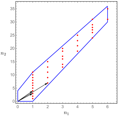
Figure 6: Blow-up divisors for the resolution of the dual of the $\mathrm{[II^{\ast}-I_{1}]}$ model. The blue solid lines join the vertices given in (6.16) for $n=1$. The red dots are the points that satisfy the coprime conditions and are thus the blow-up divisors. We show the vectors corresponding to the points $(1,3)$, $(1,4)$ and to the divisor $(2,7)$ between them, with self-intersection $-1$.

With the basic toric description at hand, we can show how the repeating blocks in the resolution in eq. (3.12) do arise and why there is a symmetry in the pattern of the self-intersections of the curves. We will consider $n\geq 1$ in what follows. To begin, we find that the $(n+1)$ divisors corresponding to $(1,5+j)$, $j=0,\ldots,n$, support type $\mathrm{II}^{*}$ fibers with self intersection number $(-11)$ for $j=0,n$, and $(-12)$ for other $j$. Next we should remember that toric information is invariant under $SL(d,\mathbb{Z})$ transformations with $d$ the dimension of the toric variety which is $2$ in our case. In particular, with

$$\left(\begin{array}[]{cc}1&0\\ -k&1\end{array}\right)$$

we can map all the ‘wedges’ spanned by $(1,6+k)$ and $(1,5+k)$ to $(1,6)$ and $(1,5)$ which shows why we obtain the same self-intersection numbers between the $(-12)$- or $(-11)$-curves. Furthermore, with

$$\left(\begin{array}[]{cc}-4-n&1\\ -6n-25&6\end{array}\right)$$

we can map the wedge spanned by $(0,1)$ and $(1,5+n)$ to $(1,6)$ and $(1,5)$. There is one further transformation,

$$\left(\begin{array}[]{cc}6&-1\\ 31&-5\end{array}\right)\,,$$

mapping $(0,-1)$, $(1,5)$ to $(1,5)$, $(1,6)$ which explains why most of the first self-intersections agree with those between the $(-12)$-curves.

To conclude with this example we give now the vectors corresponding to the (toric) blow-up divisors and their self-intersections between $(1,5)$ and $(1,6)$:

$$\{(6,31): \,-1,\,(5,26):\,-2,\,(4,21):\,-2,\,(3,16):\,-3,\,(5,27):\,-1,\,(2,11):\,-5,\,$$ (6.17)

$$(5,28):\,-1,\,(3,17):\,-3,\,(4,23):\,-2,\,(5,29):\,-2,\,(6,35):\,-1\}\,.$$

Recall that in two dimensions the self-intersection number $-a_{j}$ of a toric divisor associated to $\mathbf{n}^{j}$ satisfies $a_{j}\mathbf{n}^{j}=\mathbf{n}^{j+1}+\mathbf{n}^{j-1}$.

As a second example we want to consider the $\mathrm{[III]}$ singularity on the heterotic side, with the monodromy $\tau\rightarrow\rho$, $\rho\rightarrow\tau+\rho-2\beta$, $\beta\rightarrow\rho-\beta$. After mapping it to F-theory we obtain

$$f=u^{3}\,t^{10}(\ldots)+u^{4}\,t^{4}(\ldots)$$ (6.18)

and

$$g=u^{5}\,t^{12}(\ldots)+u^{6}\,t^{6}(\ldots)+u^{7}\,.$$ (6.19)

In addition to the positivity constraint, we get only two inequalities from $f$ and $g$,

$$(6,-1)\cdot\mathbf{n}\geq-4\,,\quad(-6,1)\cdot\mathbf{n}\geq-6\,.$$ (6.20)

These constraints are not enough to give a bounded solution set. Therefore, we will always end up with a curve of fibers which are beyond Kodaira type if we try to blow up the base to resolve the singularity at $u=t=0$. Furthermore, in this example the vanishing orders are $\mu(a)=4$, $\mu(b)=6$, $\mu(c)=10$ and $\mu(d)=12$, so that according to the criterion established before this model indeed was not expected to have a resolution.

6.2 A catalog of T-fects

We now briefly summarize the Namikawa-Ueno models for which we were able to construct the dual CY resolution. The full list of NU models is reproduced in appendix D. A simple way to determine whether a model admits a resolution is to apply the criterion stated in section 6.1, based on the vanishing orders of the coefficients $a$, $b$, $c$ and $d$ that enter in the elliptic fibration defined in equation (2.1). The model has a resolution iff $\mu(a)<4$ or $\mu(b)<6$ or $\mu(c)<10$ or $\mu(d)<12$.

6.2.1 Elliptic type 1

The elliptic type 1 models of NU are characterized by monodromies that are of finite order in the mapping class group of the genus-two surface and contain twists around the $\gamma$ cycle (see figure 1). Therefore, the corresponding action of $Sp(4,\mathbb{Z})$ elements on the Siegel upper half plane results in mixing of the $(\tau,\rho,\beta)$ moduli and the models are thus non-geometric. Disregarding the trivial monodromies, from a total of 18 types we find only 4 models whose F-theory duals admit a smooth CY resolution. We list them in table 4 together with the vanishing orders of the coefficients of the dual elliptic fibration, from which we can easily verify that the criterion discussed in the previous section is satisfied. The explicit resolutions of these models were presented in section 5.1.

NU model	$\mu(a)$	$\mu(b)$	$\mu(c)$	$\mu(d)$
$\mathrm{[I_{0-0-0}]}$	0	0	0	0
$\mathrm{[V]}$	2	3	5	6
$\mathrm{[VII]}$	2	3	5	6
$\mathrm{[VIII-1]}$	$\infty$	$\infty$	4	$\infty$
$\mathrm{[IX-1]}$	$\infty$	$\infty$	8	$\infty$

Table 4: Elliptic type 1 models.

6.2.2 Elliptic type 2

The NU list of type 2 models is given by all degenerations of type $[\mathrm{K}_{1}-\mathrm{K}_{2}-m]$, with $m\geq 0$, where $\mathrm{K}_{1}$ and $\mathrm{K}_{2}$ are one of the Kodaira type singularities for the two genus-one components of $\Sigma$, plus additional sporadic models denoted as $[2\mathrm{K}-m]$ and $[\mathrm{K}_{1}-\mathrm{K}_{2}-\alpha]$. None of the latter, nor any of the models with $m\neq 0$, give rise to smooth models. Using again the notation $[\mathrm{K}_{1}-\mathrm{K}_{2}-0]\equiv[\mathrm{K}_{1}-\mathrm{K}_{2}]$, we find a total of 20 models that satisfy our criterion, listed in table 5. As we discussed in the previous sections, the models of type $\mathrm{[I_{0}-K_{2}]}$ correspond to a configuration of $k=\mu(d)$ pointlike instantons on the $\mathrm{K_{2}}$ singularity and the resolutions are explicitly worked out in section 3.1 and in appendix A. The remaining models are non-geometric since their monodromy involves a non-trivial action on the torus volume. However, as we discussed in section 4.1 and 4.3, many of these models lead to the same resolutions as the geometric ones.

NU model	$\mu(a)$	$\mu(b)$	$\mu(c)$	$\mu(d)$	NU model	$\mu(a)$	$\mu(b)$	$\mu(c)$	$\mu(d)$
$\mathrm{[I_{0}-I_{0}]}$	0	0	0	0	$\mathrm{[II-IV]}$	3	3	6	6
$\mathrm{[I_{0}-II]}$	1	1	2	2	$\mathrm{[I_{0}^{\ast}-II]}$	3	4	8	8
$\mathrm{[I_{0}-III]}$	1	2	3	3	$\mathrm{[II-IV^{\ast}]}$	5	5	10	10
$\mathrm{[I_{0}-IV]}$	2	2	4	4	$\mathrm{[II-III^{\ast}]}$	4	7	11	11
$\mathrm{[I_{0}-I_{0}^{\ast}]}$	2	3	6	6	$\mathrm{[III-III]}$	2	4	6	6
$\mathrm{[I_{0}-IV^{\ast}]}$	4	4	8	8	$\mathrm{[IV-III]}$	3	4	7	7
$\mathrm{[I_{0}-III^{\ast}]}$	3	6	9	9	$\mathrm{[I_{0}^{\ast}-III]}$	3	5	9	9
$\mathrm{[I_{0}-II^{\ast}]}$	5	5	10	10	$\mathrm{[IV^{\ast}-III]}$	5	6	11	11
$\mathrm{[II-II]}$	2	2	4	4	$\mathrm{[IV-IV]}$	4	4	8	8
$\mathrm{[II-III]}$	2	3	5	5	$\mathrm{[I_{0}^{\ast}-IV]}$	4	5	10	10

Table 5: Elliptic type 2 models.

6.2.3 Parabolic type 3

In this class we found additional models in which the monodromy factorizes as the product of two monodromies of Kodaira type for the two tori of $\Sigma$, one of which is either $\mathrm{I}_{n}$ or $\mathrm{I}_{n}^{\ast}$ (the only parabolic elements in the Kodaira list) and the other is of elliptic type. There are also models labeled $[\mathrm{K}_{1}-\mathrm{II}_{n}]$ or $[\mathrm{K}_{1}-\mathrm{II}_{n}^{*}]$ that mix all moduli but have a Kodaira type $\mathrm{K_{1}}$ monodromy for $\tau$.

Altogether the 19 models that can be resolved are listed in table 6. These models admit a resolution for all $n$. The models of type $[\mathrm{I}_{n}-\mathrm{K}_{2}]$ or $[\mathrm{K}_{1}-\mathrm{I}_{n}]$ again correspond to $k=\mu(d)$ pointlike instantons on the $\mathrm{K}_{i}$ singularity and their resolution is shown in appendix A. The resolution for $[\mathrm{II}_{n-0}]$ and other non-trivial examples are given in section 5.2. In this class we also discover dual models. Concretely, starting with the fifth row in table 6, the models in the same row have the same resolution.

NU model	$\mu(a)$	$\mu(b)$	$\mu(c)$	$\mu(d)$	NU model	$\mu(a)$	$\mu(b)$	$\mu(c)$	$\mu(d)$
$[\mathrm{I}_{n-0-0}]$	0	0	$n$	$n$	$[\mathrm{II}-\mathrm{I}_{n}]$	$1+n$	1	$2+n$	$2+n$
$[\mathrm{III}-\mathrm{I}_{n}]$	1	$2+n$	$3+n$	$3+n$	$[\mathrm{III}-\mathrm{II}_{n}]$	1	$2+n$	$3+n$	$4+n$
$[\mathrm{IV}-\mathrm{I}_{n}]$	$2+n$	2	$4+n$	$4+n$	$[\mathrm{IV}-\mathrm{II}_{n}]$	$2+n$	2	$4+n$	$5+n$
$[\mathrm{II}_{n-0}]$	2	3	$5+n$	$6+n$
$[\mathrm{I}_{n}-\mathrm{I}_{0}^{\ast}]$	2	3	$6+n$	$6+n$	$[\mathrm{I}_{0}-\mathrm{I}_{n}^{\ast}]$	2	3	$6+n$	$6+n$
$[\mathrm{IV}^{\ast}-\mathrm{I}_{n}]$	$4+n$	4	$8+n$	$8+n$	$[\mathrm{II}-\mathrm{I}_{n}^{\ast}]$	3	4	$8+n$	$8+n$
$[\mathrm{III}^{\ast}-\mathrm{I}_{n}]$	3	$6+n$	$9+n$	$9+n$	$[\mathrm{III}-\mathrm{I}_{n}^{\ast}]$	3	5	$9+n$	$9+n$
$[\mathrm{II}^{\ast}-\mathrm{I}_{n}]$	$5+n$	5	$10+n$	$10+n$	$[\mathrm{IV}-\mathrm{I}_{n}^{\ast}]$	4	5	$10+n$	$10+n$
$[\mathrm{IV}^{\ast}-\mathrm{II}_{n}]$	$3+n$	4	$7+n$	$9+n$	$[\mathrm{II}-\mathrm{II}_{n}^{\ast}]$	$3+n$	4	$7+n$	$9+3n$
$[\mathrm{III}^{\ast}-\mathrm{II}_{n}]$	3	$5+n$	$8+n$	$11+n$	$[\mathrm{III}-\mathrm{II}_{n}^{\ast}]$	3	$5+n$	$8+n$	$10+2n$

Table 6: Parabolic type 3 models.

6.2.4 Parabolic type 4

This class includes degenerations associated to parabolic Kodaira singularities for both the genus-one components of $\Sigma$, of type $[\mathrm{K}_{1}-\mathrm{K}_{2}-m]$ with $\mathrm{K_{1,2}}=\mathrm{I}_{n},\mathrm{I}_{n}^{\ast}$, plus additional degenerations of type $[2\mathrm{K}_{1}-m]$, $[\mathrm{II}_{n-p}]$ and $[\mathrm{III}_{n}]$. We find only 3 models that admit a dual smooth resolution, listed in table 7. The explicit resolution of the $[\mathrm{I}_{n-p-0}]$ model is given in section 3.2.1, while the $[\mathrm{II}_{n-p}]$ and $[\mathrm{I}_{n}-\mathrm{I}_{p}^{\ast}]$ models are discussed in section 5.3.

NU model	$\mu(a)$	$\mu(b)$	$\mu(c)$	$\mu(d)$
$[\mathrm{I}_{n-p-0}]$	0	0	$n+p$	$n+p$
$[\mathrm{I}_{n}-\mathrm{I}_{p}^{\ast}]$	2	3	$6+n+p$	$6+n+p$
$[\mathrm{II}_{n-p}]$	2	3	$5+n+p$	$6+n+p$

Table 7: Parabolic type 4 models.

6.2.5 Parabolic type 5

The final class in the NU list is that of parabolic type 5 models, which includes just 6 degenerations. Only 2 of them admit a smooth resolution, and they are listed in table 8. The resolution of the first (geometric) model is presented in section 3.2.2. Notice that the parabolic type 5 $[\mathrm{II}_{n-p}]$ is different from the one listed in table 7. The differences between the two models are discussed in section 5.3.

NU model	$\mu(a)$	$\mu(b)$	$\mu(c)$	$\mu(d)$
$[\mathrm{I}_{n-p-q}]$	0	0	$n+p+q$	$n+p+q$
$[\mathrm{II}_{n-p}]$ $p=2k+l$, $l=0,1$	2	3	$5+l+2k+n$	$6+l+2k+n$

Table 8: Parabolic type 5 models.

This concludes the list of all genus-two degenerations in the NU list that correspond to geometric and non-geometric heterotic local models, whose F-theory duals admit a smooth resolution. Out of the 120 entries in the NU list, we find a total of 49 models.

7 Final comments

In this paper we have studied compactifications to six dimensions of the $E_{8}\times E_{8}$ heterotic string leaving an $E_{8}\times E_{7}$ subgroup unbroken. We have focused on configurations which are (up to degeneration points) locally described by a $T^{2}$ fibration over a complex one-dimensional base with a smooth $SU(2)$ structure bundle, patched together using arbitrary elements of $SO^{+}(2,3,\mathbb{Z})$ (an order four subgroup of the T-duality group $O(2,3,\mathbb{Z})$). This gives rise generically to backgrounds without a global classical geometric interpretation. At certain points in the base, the fibration (or bundle data on it) will degenerate, and will no longer have — in any T-duality frame — an interpretation in terms of the heterotic string on a smooth $T^{2}$ with a smooth vector bundle on top. Our goal in this paper has been to characterize the physics arising from such singular points.

We have made use of the fact that for backgrounds preserving $E_{8}\times E_{7}$ symmetry, the geometric data of the heterotic string on $T^{2}$ can be encoded in the geometry of a genus-two (sextic) Riemann surface. One can then define a six dimensional theory by fibering this genus-two Riemann surface over a complex one-dimensional base. For monodromies in $SO^{+}(2,3,\mathbb{Z})$, or equivalently $Sp(4,{\mathbb{Z}})$, one can classify the ways in which such fibration can degenerate [10, 11]. Using heterotic/F-theory duality to reinterpret these degenerations of the sextic as degenerations of the dual F-theory K3, fibered over the same base, we can read off the low energy physics at the degeneration point.

We have encountered two noteworthy surprises in performing the systematic analysis of the full set of degenerations of sextics. First, we have found that many, sometimes very exotic looking, non-geometric degenerations are described by the same low energy physics. Often these are given by the long-understood configurations of pointlike instantons sitting on ADE singularities. It would be very interesting to understand the origin of this phenomenon in heterotic language.

A second remarkable point is that not all of the possible degenerations of sextics admit an F-theory dual that can be smoothed out by a finite number of blow-ups. In these cases we cannot determine the low energy physics using F-theory techniques. It would be very interesting to find out which kind of SCFTs these theories might correspond to, assuming that they give consistent backgrounds. Indeed, except for the lack of smooth resolutions in the F-theory description, we have found no evidence that these backgrounds are ill-defined.

In addition to clarifying the two points just mentioned, there are various directions for further study, of which we now highlight a few. The most obvious one is probably to examine the case of non-geometric compactifications of the heterotic string down to four dimensions. Heterotic/F-theory duality will likely be an invaluable tool in this situation too.

We note that non-geometric string backgrounds have been studied in the past by a variety of approaches, and it is compelling to figure out possible implications of our concrete and explicit results for these different lines of investigation. In particular, our geometrization of the duality group contrasts with the viewpoint advocated in doubled formalisms such as double field theory [60, 61], where by extending the spacetime coordinates one finds extra degrees of freedom that need to be projected out. A potentially related question is the role of the genus-two surface in the heterotic formulation, which in a sense simultaneously encodes the physical heterotic $T^{2}$ and its T-dual. Can this genus-two curve be given a direct interpretation in the heterotic string, instead of being an auxiliary construct parameterizing the moduli space? If so, one may expect that there is some analog of the genus-two construction for heterotic compactifications breaking the symmetry further than $E_{7}\times E_{8}$. It is important to find this generalization if it exists.

Along related lines, some of our non-geometric models involve elliptic finite-order monodromies for the moduli that should admit a description in terms of asymmetric orbifolds at some point in moduli space [62, 55] and such “double elliptic” T-folds have been used in the context of generalized Scherk-Schwarz reductions [63, 54, 64].

The description of non-geometric degenerations in terms of dual F-theory models could be complemented with the explicit solutions for our T-fects. The simplest example is that of the exotic brane discussed for example in [29, 30], but it would be interesting to obtain local solutions with arbitrary $Sp(4,\mathbb{Z})$ monodromy, along the lines of [31]. Another question is how to understand in the non-geometric heterotic context the fact that 6d (1,0) superconformal field theories do not possess any marginal deformations [65, 66].

Finally, we have focused on the $E_{8}\times E_{8}$ heterotic string. Performing a similar analysis for the $SO(32)$ heterotic string is feasible, and could potentially shed some light on some of the open problems just mentioned. More ambitiously, let us mention that the same genus-two technology that has played a key role in our analysis also appears in the study of non-perturbative IIB solutions with monodromies in a subset of the U-duality group [40, 41, 42]. Understanding the physics of U-duality defects in the type II context should be very interesting. It might, for instance, be possible that U-fold defects in IIB increase the set of SCFTs constructible from F-theory beyond those considered in [14].

Acknowledgments: We are grateful to Ling Lin, Ruben Minasian, David Morrison, Erik Plauschinn, Raffaele Savelli, Stefan Theisen, Alessandro Tomasiello and Timo Weigand for useful discussions. We thank Daniel Junghans for expert nomenclature counseling. This research is supported by the Munich Excellence Cluster for Fundamental Physics “Origin and the Structure of the Universe” and by the ERC Advanced Grant 32004 – Strings and Gravity. A.F. thanks the Alexander von Humboldt Foundation for a grant VEN/1067599 STP, as well as the Max-Planck-Institut für Physik, the Ludwig-Maximillians-Universität, and the Max-Planck-Institut für Gravitationsphysik, for hospitality and support at various stages of this work. I.G.-E. and C.M. would like to thank the Aspen Center for Physics, where parts of this research were carried out, for a stimulating working atmosphere. S.M. would like to thank the Mainz Institute for Theoretical Physics (MITP) for its hospitality and its partial support during the completion of this work.

Appendix A Other ADE singularities

In this appendix we further study the local heterotic models that represent pointlike instantons on $ADE$ singularities, together with the resolutions of the dual F-theory models, from which we read the corresponding non-perturbative enhancements. This procedure was illustrated in section 3.1 for the genus-two $\mathrm{[I_{0}-II^{\ast}]}$ model, representing ten pointlike instantons on a $E_{8}$ type singularity. In sections 3.2.1 and 5.3 we also discussed the $[\mathrm{I}_{n-p-0}]$ and $[\mathrm{I}_{n}-\mathrm{I}_{p}^{*}]$ models, associated respectively to pointlike instantons on $A$ and $D$ type singularities. Here we list the remaining cases, and compare with the results of Aspinwall and Morrison for the $E_{8}\times E_{8}$ heterotic string [17].

$[\mathrm{III}^{\ast}-\mathrm{I}_{n}]$ model

For $n=0$, the local genus-two model is:

$$y^{2}=x(x^{2}+t^{3})\left(x^{2}+\alpha x+1\right)\,,$$ (A.1)

with a monodromy action given by:

$$\tau\rightarrow-\frac{1}{\tau}\,,\quad\rho\rightarrow\rho-\frac{\beta^{2}}{\tau}\,,\quad\beta\rightarrow\frac{\beta}{\tau}\,.$$ (A.2)

The geometry of the F-theory dual model, close to $u=t=0$ is:

$$f_{K3} =t^{9}u^{3}+t^{3}u^{4}\,,\quad g_{K3}=t^{9}u^{5}+t^{6}u^{6}+u^{7}\,,$$ (A.3)

$$\Delta_{K3} =-u^{9}\left(4t^{27}+12t^{21}u+27t^{18}u+66t^{15}u^{2}+27t^{12}u^{3}+58t^{9}u^{3}+54t^{6}u^{4}+27u^{5}\right)\,.$$ (A.4)

The resolution now requires a total of 14 blowups in the base and gives the following chain of Kodaira curves:

$$\mathrm{[III^{\ast}]-I_{0}-II-IV-I_{0}^{\ast}-II-IV^{\ast}-II-I_{0}^{\ast}-II-IV^{\ast}-II-I_{0}^{\ast}-IV-II}\,.$$ (A.5)

From the study of monodromy covers we then find the algebras:

12231513151322.fragments 12231513151322\begin{tabular}[]{|cccccccccccccc|}\hline\cr&&$\mathfrak{sp}(1)$&$\mathfrak{g}_{2}$&&$\mathfrak{f}_{4}$&&$\mathfrak{g}_{2}$&&$\mathfrak{f}_{4}$&&$\mathfrak{g}_{2}$&$\mathfrak{sp}(1)$&\\ 1&2&2&3&1&5&1&3&1&5&1&3&2&2\\ \hline\cr\end{tabular}\,.

sp(1)g2f4g2f4g2sp(1)sp(1)g2f4g2f4g2sp(1) (A.6)

This pattern slightly differs from the result for $k=9$ pointlike instantons on a $E_{7}$ singularity given in [17]. We actually find that the $-3$ curve at the middle supports $\mathfrak{g}_{2}$ with a fundamental $\mathbf{7}$. Each block $\mathfrak{sp}(1)\oplus\mathfrak{g}_{2}$ has matter content $\frac{1}{2}(\mathbf{2},\mathbf{1})\oplus\frac{1}{2}(\mathbf{2},\mathbf{7})$.

To obtain the case of $k=9+n$, as explained in section 3.1, we need to consider the model $[\mathrm{III}^{\ast}-\mathrm{I}_{n}]$. This introduces in the resolution a chain of $n$ $\mathrm{III^{\ast}}$ fibers which needs additional resolutions. This can be done by a total of $14+6n$ blowups and we find:

812321⊕(n−1)×\displaystyle\begin{tabular}[]{|cccccc|}\hline\cr$\mathfrak{e}_{7}$&&$\mathfrak{su}(2)$&$\mathfrak{so}(7)$&$\mathfrak{su}(2)$&\\ 8&1&2&3&2&1\\ \hline\cr\end{tabular}^{\,\oplus(n-1)}\times 8123151322.absentfragments 8123151322\displaystyle\times\begin{tabular}[]{|cccccccccc|}\hline\cr$\mathfrak{e}_{7}$&&$\mathfrak{su}(2)$&$\mathfrak{g}_{2}$&&$\mathfrak{f}_{4}$&&$\mathfrak{g}_{2}$&$\mathfrak{sp}(1)$&\\ 8&1&2&3&1&5&1&3&2&2\\ \hline\cr\end{tabular}\,.

$$\mathfrak{sp}(1)$$

1 2 2 3 1 5 1 3 2 1

e7su(2)so(7)su(2) (A.11)

e7su(2)g2f4g2sp(1)e7su(2)g2f4g2sp(1) (A.14)

The gauge algebra is now in agreement with [17]. There is matter only for the $\mathfrak{sp}(1)\oplus\mathfrak{g}_{2}$ and $\mathfrak{su}(2)\oplus\mathfrak{so}(7)\oplus\mathfrak{su}(2)$ clusters. Concretely, $\frac{1}{2}(\mathbf{2},\mathbf{1})\oplus\frac{1}{2}(\mathbf{2},\mathbf{7})$ for the former and $\frac{1}{2}(\mathbf{2},\mathbf{8},\mathbf{1})\oplus\frac{1}{2}(\mathbf{1},\mathbf{8},\mathbf{2})$ for the latter.

$[\mathrm{IV}^{\ast}-\mathrm{I}_{n}]$ model

The local $[\mathrm{I}_{0}-\mathrm{IV}^{\ast}]$ NU model is:

$$y^{2}=(x^{3}+t^{4})(x^{2}+\alpha x+1)\,,$$ (A.15)

with monodromy

$$\tau\rightarrow-\frac{1+\tau}{\tau}\,,\quad\rho\rightarrow\rho-\frac{\beta^{2}}{\tau}\,,\quad\beta\rightarrow\frac{\beta}{\tau}\,.$$ (A.16)

The geometry of the F-theory dual model, close to $u=t=0$ is schematically:

$$f_{K3} =t^{8}u^{3}+t^{4}u^{4}\,,\quad g_{K3}=t^{8}u^{5}+t^{4}u^{6}+u^{7}\,,$$ (A.17)

$$\Delta_{K3} =-u^{9}\left(4t^{24}+12t^{20}u+12t^{16}u^{2}+27t^{16}u+4t^{12}u^{3}+54t^{12}u^{2}+81t^{8}u^{3}+54t^{4}u^{4}+27u^{5}\right)\,.$$

We now get the following chain:

$$\mathrm{[III^{\ast}]-I_{0}-II-IV-I_{0}^{\ast}-II-IV^{\ast}-II-I_{0}^{\ast}-IV-II}\,,$$ (A.18)

from which we determine the gauge algebra:

1223141322,fragments 1223141322\begin{tabular}[]{|cccccccccc|}\hline\cr&&$\mathfrak{sp}(1)$&$\mathfrak{g}_{2}$&&$\mathfrak{f}_{4}$&&$\mathfrak{g}_{2}$&$\mathfrak{sp}(1)$&\\ 1&2&2&3&1&4&1&3&2&2\\ \hline\cr\end{tabular}\,,

sp(1)g2f4g2sp(1)sp(1)g2f4g2sp(1) (A.19)

giving the theory of 8 pointlike instantons on the $E_{6}$ singularity. As before, matter for $\mathfrak{sp}(1)\oplus\mathfrak{g}_{2}$ consists of $\frac{1}{2}(\mathbf{2},\mathbf{1})\oplus\frac{1}{2}(\mathbf{2},\mathbf{7})$. We find an extra fundamental for the $\mathfrak{f}_{4}$ with self-intersection $-4$.

The model $[\mathrm{IV}^{\ast}-\mathrm{I}_{n}]$, $n\geq 1$, introduces a chain of $\mathrm{IV^{\ast}}$ fibers, whose resolution requires a total of $10+4n$ blowups:

122315131​ 6131⊗(n−1)​ 51322.fragments 122315131superscriptfragments 6131tensor-productabsent𝑛1fragments 51322\begin{tabular}[]{|ccccccccc|}\hline\cr&&$\mathfrak{sp}(1)$&$\mathfrak{g}_{2}$&&$\mathfrak{f}_{4}$&&$\mathfrak{su}(3)$&\\ 1&2&2&3&1&5&1&3&1\\ \hline\cr\end{tabular}\,\begin{tabular}[]{|cccc|}\hline\cr$\mathfrak{e}_{6}$&&$\mathfrak{su}(3)$&\\ 6&1&3&1\\ \hline\cr\end{tabular}^{\,\otimes(n-1)}\,\begin{tabular}[]{|ccccc|}\hline\cr$\mathfrak{f}_{4}$&&$\mathfrak{g}_{2}$&$\mathfrak{sp}(1)$&\\ 5&1&3&2&2\\ \hline\cr\end{tabular}\,.

sp(1)g2f4su(3)e6su(3)f4g2sp(1)sp(1)g2f4su(3)e6su(3)f4g2sp(1) (A.20)

This gives the theory of $k=8+n$ pointlike instantons, as originally found in [17]. The only matter is $\frac{1}{2}(\mathbf{2},\mathbf{1})\oplus\frac{1}{2}(\mathbf{2},\mathbf{7})$ for each $\mathfrak{sp}(1)\oplus\mathfrak{g}_{2}$ block.

$[\mathrm{I}_{0}^{\ast}-\mathrm{I}_{n}]$ model

The local model for $n=0$ is:

$$y^{2}=(x^{3}+\beta t^{2}x+t^{3})(x^{3}+\alpha x+1)\,.$$ (A.21)

The monodromy action on the moduli leaves $\tau$ and $\rho$ invariant, while it acts on the Wilson line as $\beta\rightarrow-\beta$. The geometry of the F-theory dual model, close to $u=t=0$ is:

$$f_{K3} =t^{6}u^{3}+t^{2}u^{4}\,,\quad g_{K3}=t^{6}u^{5}+t^{3}u^{6}+u^{7}\,,$$ (A.22)

$$\Delta_{K3} =-u^{9}\left(4t^{18}+12t^{14}u+27t^{12}u+12t^{10}u^{2}+54t^{9}u^{2}+85t^{6}u^{3}+54t^{3}u^{4}+27u^{5}\right)\,.$$ (A.23)

We get the following resolution:

$$\mathrm{[III^{\ast}]-I_{0}-II-IV-I_{0}^{\ast}-IV-II}\,,$$ (A.24)

and we find the algebra

122222,fragments 122222\begin{tabular}[]{|cccccc|}\hline\cr&&$\mathfrak{sp}(1)$&$\mathfrak{g}_{2}$&$\mathfrak{sp}(1)$&\\ 1&2&2&2&2&2\\ \hline\cr\end{tabular}\,,

sp(1)g2sp(1)sp(1)g2sp(1) (A.25)

which gives the non-perturbative enhancement for $k=6$ pointlike instantons on a $D_{4}$ singularity. The gauge factors and the matter representations are the same as in the $\mathrm{III}-\mathrm{III}$ model presented in section 4.1.

Adding $n$ more instantons, thus considering the $[\mathrm{I}_{0}^{\ast}-\mathrm{I}_{n}]$ model, results in a chain of additional $n$ $\mathrm{I}_{0}^{\ast}$ singularities, whose resolution gives:

12231​ 41⊕(n−1)​ 322,fragments 12231superscriptfragments 41direct-sum𝑛1fragments 322\begin{tabular}[]{|ccccc|}\hline\cr&&$\mathfrak{sp}(1)$&$\mathfrak{g}_{2}$&\\ 1&2&2&3&1\\ \hline\cr\end{tabular}\,\begin{tabular}[]{|cc|}\hline\cr$\mathfrak{so}(8)$&\\ 4&1\\ \hline\cr\end{tabular}^{\,\oplus(n-1)}\,\begin{tabular}[]{|ccc|}\hline\cr$\mathfrak{g}_{2}$&$\mathfrak{sp}(1)$&\\ 3&2&2\\ \hline\cr\end{tabular}\,,

sp(1)g2so(8)g2sp(1)sp(1)g2so(8)g2sp(1) (A.26)

for a total of $6+2n$ blowups. Matter is just $\frac{1}{2}(\mathbf{2},\mathbf{1})\oplus\frac{1}{2}(\mathbf{2},\mathbf{7})$ for each $\mathfrak{sp}(1)\oplus\mathfrak{g}_{2}$ cluster.

$[\mathrm{IV}-\mathrm{I}_{n}]$ model

The local model for $\mathrm{[I_{0}-IV]}$ is:

$$y^{2}=(x^{3}+t^{2})(x^{3}+\alpha x+1)\,,$$ (A.27)

with monodromy action

$$\tau\rightarrow-\frac{1}{1+\tau}\,,\quad\rho\rightarrow\rho-\frac{\beta^{2}}{1+\tau}\,,\quad\beta\rightarrow-\frac{\beta}{1+\tau}\,.$$ (A.28)

The geometry of the F-theory dual model, close to $u=t=0$ is:

$$f_{K3} =t^{4}u^{3}+t^{2}u^{4}\,,\quad g_{K3}=t^{4}u^{5}+t^{2}u^{6}+u^{7}\,,$$ (A.29)

$$\Delta_{K3} =-u^{9}\left(4t^{12}+12t^{10}u+12t^{8}u^{2}+27t^{8}u+4t^{6}u^{3}+54t^{6}u^{2}+81t^{4}u^{3}+54t^{2}u^{4}+27u^{5}\right)\,.$$

From the resolution we get the following chain:

$$\mathrm{[III^{\ast}]-I_{0}-II-IV-II}\,,$$ (A.30)

and gauge algebra:

1222.fragments 1222\begin{tabular}[]{|cccc|}\hline\cr&&$\mathfrak{sp}(1)$&\\ 1&2&2&2\\ \hline\cr\end{tabular}\,.

sp(1)sp(1) (A.31)

From the $[\mathrm{IV}-\mathrm{I}_{n}]$ model we get $n$ additional $\mathrm{IV}$ fibers and we recover the theory for $k=4+n$ pointlike instantons:

1222⋯222,fragments 1222⋯222\begin{tabular}[]{|cccccccc|}\hline\cr&&$\mathfrak{sp}(1)$&$\mathfrak{su}(3)_{1}$&&$\mathfrak{su}(3)_{n-1}$&$\mathfrak{sp}(1)$&\\ 1&2&2&2&$\cdots$&2&2&2\\ \hline\cr\end{tabular}\,,

sp(1)su(3)1su(3)-n1sp(1)sp(1)su(3)1su(3)-n1sp(1) (A.32)

which again agrees with [17]. Matter consists of bifundamentals for adjacent $\mathfrak{su}(3)$’s, together with $(\mathbf{2},\mathbf{1})\oplus(\mathbf{2}+\mathbf{1},\mathbf{3})$ for the $\mathfrak{sp}(1)\oplus\mathfrak{su}(3)$’s at the corners.

$[\mathrm{III}-\mathrm{I}_{n}]$ model

For this final example we skip the details. The resolution is found to be:

1222⋯22,fragments 1222⋯22\begin{tabular}[]{|ccccccc|}\hline\cr&&$\mathfrak{su}(2)_{1}$&$\mathfrak{su}(2)_{2}$&&$\mathfrak{su}(2)_{n}$&\\ 1&2&2&2&$\cdots$&2&2\\ \hline\cr\end{tabular}\,,

su(2)1su(2)2su(2)nsu(2)1su(2)2su(2)n (A.33)

Matter is given by bifundamentals for neighboring factors, plus two additional fundamentals for the left- and right-most $\mathfrak{su}(2)$’s.

Appendix B Map for vanishing Wilson line

In this section we consider the duality map (2.6) in the limit $\beta\rightarrow 0$. This corresponds to the splitting of the genus-two curve into two tori, whose mapping class groups geometrize the $SL(2,\mathbb{Z})_{\tau}\times SL(2,\mathbb{Z})_{\rho}$ subgroup of the $O(2,2,\mathbb{Z})$ T-duality group in the absence of Wilson lines (see Figure 1).

From [4], we have that, setting $\beta=0$:

$$a=-\frac{E_{4}(\tau)E_{4}(\rho)}{48}\,,\quad b=-\frac{E_{6}(\tau)E_{6}(\rho)}{864}\,,\quad c=0\,,\quad d=\eta(\tau)^{24}\eta(\rho)^{24}\,.$$ (B.1)

Here $E_{4}$ and $E_{6}$ are the modular forms of weights four and six for the two $SL(2,\mathbb{Z})$ groups and $\eta$ is the Dedekind $\eta$-function. In fact, this form of the duality map agrees with the formulation in [3], based on the construction of a Shioda-Inose structure for the K3 surface [6]. The data about the $\tau$ and $\rho$ moduli can be encoded in two Weierstraß equations that describe the two genus-one components of the split genus-two curve:

$$y^{2}=x^{3}+f_{\tau}x\,w^{4}+g_{\tau}w^{6}\,,\quad\tilde{y}^{2}=\tilde{x}^{3}+f_{\rho}\tilde{x}\,\tilde{w}^{4}+g_{\rho}\tilde{w}^{6}\,,$$ (B.2)

by the identifications

$$f=-\frac{1}{3}E_{4}\,,\quad g=-\frac{2}{27}E_{6}\,,\quad\eta^{24}=-\frac{27}{4}\frac{\Delta}{1728}\,,$$ (B.3)

where $\Delta=4f^{3}+27g^{2}$ is the discriminant of the Weierstraß equation. We thus get that the dual K3 is described by

$$y^{2}=x^{3}-\frac{3}{16}f_{\tau}f_{\rho}xu^{4}w^{4}+\frac{\Delta_{\tau}\Delta_{\rho}}{16^{4}}u^{5}w^{6}-\frac{27}{128}g_{\tau}g_{\rho}u^{6}w^{6}+u^{7}w^{6}\,.$$ (B.4)

It is easy to show that this indeed satisfies the relations (2.2), originally obtained in [9]. After a rescaling $(u,w)\rightarrow(2^{-6}u,2^{7}w)$ we find

$$y^{2}=x^{3}-3f_{\tau}f_{\rho}xu^{4}w^{4}+\frac{\Delta_{\tau}\Delta_{\rho}}{16}u^{5}w^{6}-\frac{27}{2}g_{\tau}g_{\rho}u^{6}w^{6}+u^{7}w^{6}\,,$$ (B.5)

which is a particular case of the expression given in [3]. More generally, one can allow the coefficient of the $u^{7}$ term to transform as a section of a nontrivial line bundle, corresponding to a different distribution of the point-like instantons between the two $E_{8}$ factors. The map (B.5) is modified as follows:

$$y^{2}=x^{3}-3f_{\tau}f_{\rho}xu^{4}w^{4}+d_{\tau}d_{\rho}u^{5}w^{6}-\frac{27}{2}g_{\tau}g_{\rho}u^{6}w^{6}+e_{\tau}e_{\rho}u^{7}w^{6}\,,$$ (B.6)

where $\Delta_{\tau}=4d_{\tau}e_{\tau}$ and $\Delta_{\rho}=4d_{\rho}e_{\rho}$.

As a check, one can obtain the resolution for the dual of the NU model $[\mathrm{I}_{n}-\mathrm{II}^{\ast}]$ in the $\beta\rightarrow 0$ limit by using (B.6). For this we can take for example $f_{\tau}=t^{4}$, $g_{\tau}=t^{5}$, $f_{\rho}=-3$, $g_{\rho}=2+t^{n}$, and set $d_{\tau}=t^{5}$, $e_{\tau}=t^{5}(27+4t^{2})$, $d_{\rho}=27t^{n}$, $e_{\rho}=4+t^{n}$. With this choice we engineer $\mathrm{II}^{\ast}$ and $\mathrm{I}_{n}$ singularities in $\tau$ and $\rho$, respectively. We then find that at $t=0$ there is a “vertical” $\mathrm{II^{\ast}}$ fiber intersecting the two “horizontal” $\mathrm{II^{\ast}}$ fibers at $u=0$ and $v=0$, with additional $n$ instantons coalesced at the $u=t=0$ intersection [17]. Resolving both intersections at $u=t=0$ and $v=t=0$ gives precisely the chain derived in section 3.1, corresponding to $10+n$ pointlike instantons on top of the $E_{8}$ singularity.

Appendix C Igusa-Clebsch invariants

We collect here the expressions of the Igusa-Clebsch invariants for an hyperelliptic curve in terms of the coefficients of the general sextic (2.7). Similar formulas have appeared in [67].

$$I_{2} =6c_{3}^{2}-16c_{2}c_{4}+40c_{1}c_{5}-240c_{0}c_{6}\,,$$ (C.1)

$$I_{4} =48c_{6}c_{2}^{3}+4c_{4}^{2}c_{2}^{2}-12c_{3}c_{5}c_{2}^{2}+300c_{0}c_{5}^{2}c_{2}+4c_{1}c_{4}c_{5}c_{2}-180c_{1}c_{3}c_{6}c_{2}-504c_{0}c_{4}c_{6}c_{2}+48c_{0}c_{4}^{3}-12c_{1}c_{3}c_{4}^{2}-80c_{1}^{2}c_{5}^{2}$$

$$\quad+1620c_{0}^{2}c_{6}^{2}+36c_{1}c_{3}^{2}c_{5}-180c_{0}c_{3}c_{4}c_{5}+324c_{0}c_{3}^{2}c_{6}+300c_{1}^{2}c_{4}c_{6}-540c_{0}c_{1}c_{5}c_{6}\,,$$ (C.2)

$$I_{6} =-36c_{5}^{2}c_{2}^{4}-160c_{4}c_{6}c_{2}^{4}-24c_{4}^{3}c_{2}^{3}-96c_{0}c_{6}^{2}c_{2}^{3}+76c_{3}c_{4}c_{5}c_{2}^{3}+60c_{3}^{2}c_{6}c_{2}^{3}+616c_{1}c_{5}c_{6}c_{2}^{3}+8c_{3}^{2}c_{4}^{2}c_{2}^{2}+26c_{1}c_{3}c_{5}^{2}c_{2}^{2}$$

$$\quad-640c_{0}c_{4}c_{5}^{2}c_{2}^{2}-900c_{1}^{2}c_{6}^{2}c_{2}^{2}-24c_{3}^{3}c_{5}c_{2}^{2}+28c_{1}c_{4}^{2}c_{5}c_{2}^{2}+424c_{0}c_{4}^{2}c_{6}c_{2}^{2}+492c_{1}c_{3}c_{4}c_{6}c_{2}^{2}-876c_{0}c_{3}c_{5}c_{6}c_{2}^{2}$$

$$\quad-160c_{0}c_{4}^{4}c_{2}+76c_{1}c_{3}c_{4}^{3}c_{2}+1600c_{0}c_{1}c_{5}^{3}c_{2}+330c_{0}c_{3}^{2}c_{5}^{2}c_{2}+64c_{1}^{2}c_{4}c_{5}^{2}c_{2}+3060c_{0}c_{1}c_{3}c_{6}^{2}c_{2}+20664c_{0}^{2}c_{4}c_{6}^{2}c_{2}$$

$$\quad+492c_{0}c_{3}c_{4}^{2}c_{5}c_{2}-238c_{1}c_{3}^{2}c_{4}c_{5}c_{2}-198c_{1}c_{3}^{3}c_{6}c_{2}-640c_{1}^{2}c_{4}^{2}c_{6}c_{2}-18600c_{0}^{2}c_{5}^{2}c_{6}c_{2}-468c_{0}c_{3}^{2}c_{4}c_{6}c_{2}-1860c_{1}^{2}c_{3}c_{5}c_{6}c_{2}$$

$$\quad+3472c_{0}c_{1}c_{4}c_{5}c_{6}c_{2}-36c_{1}^{2}c_{4}^{4}+60c_{0}c_{3}^{2}c_{4}^{3}-320c_{1}^{3}c_{5}^{3}+2250c_{0}^{2}c_{3}c_{5}^{3}-119880c_{0}^{3}c_{6}^{3}-24c_{1}c_{3}^{3}c_{4}^{2}+176c_{1}^{2}c_{3}^{2}c_{5}^{2}-900c_{0}^{2}c_{4}^{2}c_{5}^{2}$$

$$\quad-1860c_{0}c_{1}c_{3}c_{4}c_{5}^{2}-10044c_{0}^{2}c_{3}^{2}c_{6}^{2}+2250c_{1}^{3}c_{3}c_{6}^{2}-18600c_{0}c_{1}^{2}c_{4}c_{6}^{2}+59940c_{0}^{2}c_{1}c_{5}c_{6}^{2}+72c_{1}c_{3}^{4}c_{5}+616c_{0}c_{1}c_{4}^{3}c_{5}$$

$$\quad+26c_{1}^{2}c_{3}c_{4}^{2}c_{5}-198c_{0}c_{3}^{3}c_{4}c_{5}+162c_{0}c_{3}^{4}c_{6}-96c_{0}^{2}c_{4}^{3}c_{6}-876c_{0}c_{1}c_{3}c_{4}^{2}c_{6}-2240c_{0}c_{1}^{2}c_{5}^{2}c_{6}+330c_{1}^{2}c_{3}^{2}c_{4}c_{6}$$

$$\quad+1818c_{0}c_{1}c_{3}^{2}c_{5}c_{6}+1600c_{1}^{3}c_{4}c_{5}c_{6}+3060c_{0}^{2}c_{3}c_{4}c_{5}c_{6}\,,$$ (C.3)

$$I_{10} =3125c_{6}^{4}c_{1}^{6}+256c_{5}^{5}c_{1}^{5}-3750c_{3}c_{4}c_{6}^{3}c_{1}^{5}-2500c_{2}c_{5}c_{6}^{3}c_{1}^{5}+2000c_{3}c_{5}^{2}c_{6}^{2}c_{1}^{5}+2250c_{4}^{2}c_{5}c_{6}^{2}c_{1}^{5}-1600c_{4}c_{5}^{3}c_{6}c_{1}^{5}-128c_{3}^{2}c_{5}^{4}c_{1}^{4}$$

$$\quad-192c_{2}c_{4}c_{5}^{4}c_{1}^{4}-22500c_{0}c_{2}c_{6}^{4}c_{1}^{4}+144c_{3}c_{4}^{2}c_{5}^{3}c_{1}^{4}+2250c_{2}c_{3}^{2}c_{6}^{3}c_{1}^{4}+1500c_{0}c_{4}^{2}c_{6}^{3}c_{1}^{4}+2000c_{2}^{2}c_{4}c_{6}^{3}c_{1}^{4}+2250c_{0}c_{3}c_{5}c_{6}^{3}c_{1}^{4}$$

$$\quad-27c_{4}^{4}c_{5}^{2}c_{1}^{4}-900c_{2}c_{4}^{3}c_{6}^{2}c_{1}^{4}+825c_{3}^{2}c_{4}^{2}c_{6}^{2}c_{1}^{4}-50c_{2}^{2}c_{5}^{2}c_{6}^{2}c_{1}^{4}-1700c_{0}c_{4}c_{5}^{2}c_{6}^{2}c_{1}^{4}-900c_{3}^{3}c_{5}c_{6}^{2}c_{1}^{4}-2050c_{2}c_{3}c_{4}c_{5}c_{6}^{2}c_{1}^{4}$$

$$\quad+108c_{4}^{5}c_{6}c_{1}^{4}+320c_{0}c_{5}^{4}c_{6}c_{1}^{4}+160c_{2}c_{3}c_{5}^{3}c_{6}c_{1}^{4}+1020c_{2}c_{4}^{2}c_{5}^{2}c_{6}c_{1}^{4}+560c_{3}^{2}c_{4}c_{5}^{2}c_{6}c_{1}^{4}-630c_{3}c_{4}^{3}c_{5}c_{6}c_{1}^{4}-1600c_{0}c_{2}c_{5}^{5}c_{1}^{3}$$

$$\quad+144c_{2}^{2}c_{3}c_{5}^{4}c_{1}^{3}+160c_{0}c_{3}c_{4}c_{5}^{4}c_{1}^{3}+27000c_{0}^{2}c_{3}c_{6}^{4}c_{1}^{3}+16c_{3}^{4}c_{5}^{3}c_{1}^{3}-36c_{0}c_{4}^{3}c_{5}^{3}c_{1}^{3}-6c_{2}^{2}c_{4}^{2}c_{5}^{3}c_{1}^{3}-80c_{2}c_{3}^{2}c_{4}c_{5}^{3}c_{1}^{3}-1350c_{0}c_{3}^{3}c_{6}^{3}c_{1}^{3}$$

$$\quad-1600c_{2}^{3}c_{3}c_{6}^{3}c_{1}^{3}+19800c_{0}c_{2}c_{3}c_{4}c_{6}^{3}c_{1}^{3}+15600c_{0}c_{2}^{2}c_{5}c_{6}^{3}c_{1}^{3}-1800c_{0}^{2}c_{4}c_{5}c_{6}^{3}c_{1}^{3}+18c_{2}c_{3}c_{4}^{3}c_{5}^{2}c_{1}^{3}-4c_{3}^{3}c_{4}^{2}c_{5}^{2}c_{1}^{3}+108c_{3}^{5}c_{6}^{2}c_{1}^{3}$$

$$\quad-120c_{0}c_{3}c_{4}^{3}c_{6}^{2}c_{1}^{3}+410c_{0}^{2}c_{5}^{3}c_{6}^{2}c_{1}^{3}+560c_{2}^{2}c_{3}c_{4}^{2}c_{6}^{2}c_{1}^{3}-12330c_{0}c_{2}c_{3}c_{5}^{2}c_{6}^{2}c_{1}^{3}-630c_{2}c_{3}^{3}c_{4}c_{6}^{2}c_{1}^{3}+1020c_{2}^{2}c_{3}^{2}c_{5}c_{6}^{2}c_{1}^{3}$$

$$\quad-13040c_{0}c_{2}c_{4}^{2}c_{5}c_{6}^{2}c_{1}^{3}+160c_{2}^{3}c_{4}c_{5}c_{6}^{2}c_{1}^{3}+1980c_{0}c_{3}^{2}c_{4}c_{5}c_{6}^{2}c_{1}^{3}-72c_{2}c_{3}c_{4}^{4}c_{6}c_{1}^{3}+16c_{3}^{3}c_{4}^{3}c_{6}c_{1}^{3}-36c_{2}^{3}c_{5}^{3}c_{6}c_{1}^{3}-208c_{0}c_{3}^{2}c_{5}^{3}c_{6}c_{1}^{3}$$

$$\quad+9768c_{0}c_{2}c_{4}c_{5}^{3}c_{6}c_{1}^{3}+24c_{2}c_{3}^{3}c_{5}^{2}c_{6}c_{1}^{3}-682c_{0}c_{3}c_{4}^{2}c_{5}^{2}c_{6}c_{1}^{3}-746c_{2}^{2}c_{3}c_{4}c_{5}^{2}c_{6}c_{1}^{3}+144c_{0}c_{4}^{4}c_{5}c_{6}c_{1}^{3}+24c_{2}^{2}c_{4}^{3}c_{5}c_{6}c_{1}^{3}$$

$$\quad+356c_{2}c_{3}^{2}c_{4}^{2}c_{5}c_{6}c_{1}^{3}-72c_{3}^{4}c_{4}c_{5}c_{6}c_{1}^{3}+2000c_{0}^{2}c_{3}c_{5}^{5}c_{1}^{2}-27c_{2}^{4}c_{5}^{4}c_{1}^{2}+560c_{0}c_{2}c_{3}^{2}c_{5}^{4}c_{1}^{2}-50c_{0}^{2}c_{4}^{2}c_{5}^{4}c_{1}^{2}+1020c_{0}c_{2}^{2}c_{4}c_{5}^{4}c_{1}^{2}$$

$$\quad+43200c_{0}^{2}c_{2}^{2}c_{6}^{4}c_{1}^{2}-32400c_{0}^{3}c_{4}c_{6}^{4}c_{1}^{2}-4c_{2}^{2}c_{3}^{3}c_{5}^{3}c_{1}^{2}-746c_{0}c_{2}c_{3}c_{4}^{2}c_{5}^{3}c_{1}^{2}+24c_{0}c_{3}^{3}c_{4}c_{5}^{3}c_{1}^{2}+18c_{2}^{3}c_{3}c_{4}c_{5}^{3}c_{1}^{2}+256c_{2}^{5}c_{6}^{3}c_{1}^{2}$$

$$\quad-9720c_{0}c_{2}^{2}c_{3}^{2}c_{6}^{3}c_{1}^{2}-6480c_{0}^{2}c_{2}c_{4}^{2}c_{6}^{3}c_{1}^{2}+540c_{0}^{3}c_{5}^{2}c_{6}^{3}c_{1}^{2}-10560c_{0}c_{2}^{3}c_{4}c_{6}^{3}c_{1}^{2}-27540c_{0}^{2}c_{3}^{2}c_{4}c_{6}^{3}c_{1}^{2}-31320c_{0}^{2}c_{2}c_{3}c_{5}c_{6}^{3}c_{1}^{2}$$

$$\quad+144c_{0}c_{2}c_{4}^{4}c_{5}^{2}c_{1}^{2}-4c_{2}^{3}c_{4}^{3}c_{5}^{2}c_{1}^{2}-6c_{0}c_{3}^{2}c_{4}^{3}c_{5}^{2}c_{1}^{2}+c_{2}^{2}c_{3}^{2}c_{4}^{2}c_{5}^{2}c_{1}^{2}-27c_{2}^{2}c_{3}^{4}c_{6}^{2}c_{1}^{2}-192c_{0}^{2}c_{4}^{4}c_{6}^{2}c_{1}^{2}+4816c_{0}c_{2}^{2}c_{4}^{3}c_{6}^{2}c_{1}^{2}$$

$$\quad-128c_{2}^{4}c_{4}^{2}c_{6}^{2}c_{1}^{2}-4536c_{0}c_{2}c_{3}^{2}c_{4}^{2}c_{6}^{2}c_{1}^{2}+248c_{0}c_{2}^{3}c_{5}^{2}c_{6}^{2}c_{1}^{2}+15417c_{0}^{2}c_{3}^{2}c_{5}^{2}c_{6}^{2}c_{1}^{2}+8748c_{0}^{2}c_{2}c_{4}c_{5}^{2}c_{6}^{2}c_{1}^{2}+162c_{0}c_{3}^{4}c_{4}c_{6}^{2}c_{1}^{2}$$

$$\quad+144c_{2}^{3}c_{3}^{2}c_{4}c_{6}^{2}c_{1}^{2}+3942c_{0}c_{2}c_{3}^{3}c_{5}c_{6}^{2}c_{1}^{2}+16632c_{0}^{2}c_{3}c_{4}^{2}c_{5}c_{6}^{2}c_{1}^{2}-192c_{2}^{4}c_{3}c_{5}c_{6}^{2}c_{1}^{2}+10152c_{0}c_{2}^{2}c_{3}c_{4}c_{5}c_{6}^{2}c_{1}^{2}-576c_{0}c_{2}c_{4}^{5}c_{6}c_{1}^{2}$$

$$\quad+16c_{2}^{3}c_{4}^{4}c_{6}c_{1}^{2}+24c_{0}c_{3}^{2}c_{4}^{4}c_{6}c_{1}^{2}-1700c_{0}^{2}c_{2}c_{5}^{4}c_{6}c_{1}^{2}-4c_{2}^{2}c_{3}^{2}c_{4}^{3}c_{6}c_{1}^{2}-682c_{0}c_{2}^{2}c_{3}c_{5}^{3}c_{6}c_{1}^{2}-12330c_{0}^{2}c_{3}c_{4}c_{5}^{3}c_{6}c_{1}^{2}$$

$$\quad+248c_{0}^{2}c_{4}^{3}c_{5}^{2}c_{6}c_{1}^{2}-6c_{2}^{3}c_{3}^{2}c_{5}^{2}c_{6}c_{1}^{2}-5428c_{0}c_{2}^{2}c_{4}^{2}c_{5}^{2}c_{6}c_{1}^{2}+144c_{2}^{4}c_{4}c_{5}^{2}c_{6}c_{1}^{2}-2412c_{0}c_{2}c_{3}^{2}c_{4}c_{5}^{2}c_{6}c_{1}^{2}+3272c_{0}c_{2}c_{3}c_{4}^{3}c_{5}c_{6}c_{1}^{2}$$

$$\quad-108c_{0}c_{3}^{3}c_{4}^{2}c_{5}c_{6}c_{1}^{2}-80c_{2}^{3}c_{3}c_{4}^{2}c_{5}c_{6}c_{1}^{2}+18c_{2}^{2}c_{3}^{3}c_{4}c_{5}c_{6}c_{1}^{2}+2250c_{0}^{2}c_{2}^{2}c_{5}^{5}c_{1}-2500c_{0}^{3}c_{4}c_{5}^{5}c_{1}-900c_{0}^{2}c_{3}^{3}c_{5}^{4}c_{1}-630c_{0}c_{2}^{3}c_{3}c_{5}^{4}c_{1}$$

$$\quad-2050c_{0}^{2}c_{2}c_{3}c_{4}c_{5}^{4}c_{1}-77760c_{0}^{3}c_{2}c_{3}c_{6}^{4}c_{1}+38880c_{0}^{4}c_{5}c_{6}^{4}c_{1}-72c_{0}c_{2}c_{3}^{4}c_{5}^{3}c_{1}+160c_{0}^{2}c_{2}c_{4}^{3}c_{5}^{3}c_{1}+24c_{0}c_{2}^{3}c_{4}^{2}c_{5}^{3}c_{1}$$

$$\quad+1020c_{0}^{2}c_{3}^{2}c_{4}^{2}c_{5}^{3}c_{1}+356c_{0}c_{2}^{2}c_{3}^{2}c_{4}c_{5}^{3}c_{1}+21384c_{0}^{2}c_{2}c_{3}^{3}c_{6}^{3}c_{1}+46656c_{0}^{3}c_{3}c_{4}^{2}c_{6}^{3}c_{1}+6912c_{0}c_{2}^{4}c_{3}c_{6}^{3}c_{1}-3456c_{0}^{2}c_{2}^{2}c_{3}c_{4}c_{6}^{3}c_{1}$$

$$\quad-21888c_{0}^{2}c_{2}^{3}c_{5}c_{6}^{3}c_{1}+15552c_{0}^{3}c_{3}^{2}c_{5}c_{6}^{3}c_{1}+31968c_{0}^{3}c_{2}c_{4}c_{5}c_{6}^{3}c_{1}-192c_{0}^{2}c_{3}c_{4}^{4}c_{5}^{2}c_{1}-80c_{0}c_{2}^{2}c_{3}c_{4}^{3}c_{5}^{2}c_{1}+18c_{0}c_{2}c_{3}^{3}c_{4}^{2}c_{5}^{2}c_{1}$$

$$\quad-486c_{0}c_{2}c_{3}^{5}c_{6}^{2}c_{1}-5760c_{0}^{2}c_{2}c_{3}c_{4}^{3}c_{6}^{2}c_{1}-1800c_{0}^{3}c_{2}c_{5}^{3}c_{6}^{2}c_{1}+5832c_{0}^{2}c_{3}^{3}c_{4}^{2}c_{6}^{2}c_{1}-2496c_{0}c_{2}^{3}c_{3}c_{4}^{2}c_{6}^{2}c_{1}+16632c_{0}^{2}c_{2}^{2}c_{3}c_{5}^{2}c_{6}^{2}c_{1}$$

$$\quad-31320c_{0}^{3}c_{3}c_{4}c_{5}^{2}c_{6}^{2}c_{1}+2808c_{0}c_{2}^{2}c_{3}^{3}c_{4}c_{6}^{2}c_{1}-6318c_{0}^{2}c_{3}^{4}c_{5}c_{6}^{2}c_{1}-21888c_{0}^{3}c_{4}^{3}c_{5}c_{6}^{2}c_{1}-4464c_{0}c_{2}^{3}c_{3}^{2}c_{5}c_{6}^{2}c_{1}$$

$$\quad+15264c_{0}^{2}c_{2}^{2}c_{4}^{2}c_{5}c_{6}^{2}c_{1}-640c_{0}c_{2}^{4}c_{4}c_{5}c_{6}^{2}c_{1}-22896c_{0}^{2}c_{2}c_{3}^{2}c_{4}c_{5}c_{6}^{2}c_{1}+768c_{0}^{2}c_{3}c_{4}^{5}c_{6}c_{1}+320c_{0}c_{2}^{2}c_{3}c_{4}^{4}c_{6}c_{1}+2250c_{0}^{3}c_{3}c_{5}^{4}c_{6}c_{1}$$

$$\quad-72c_{0}c_{2}c_{3}^{3}c_{4}^{3}c_{6}c_{1}+144c_{0}c_{2}^{4}c_{5}^{3}c_{6}c_{1}+1980c_{0}^{2}c_{2}c_{3}^{2}c_{5}^{3}c_{6}c_{1}+15600c_{0}^{3}c_{4}^{2}c_{5}^{3}c_{6}c_{1}-13040c_{0}^{2}c_{2}^{2}c_{4}c_{5}^{3}c_{6}c_{1}-108c_{0}c_{2}^{2}c_{3}^{3}c_{5}^{2}c_{6}c_{1}$$

$$\quad+10152c_{0}^{2}c_{2}c_{3}c_{4}^{2}c_{5}^{2}c_{6}c_{1}+3942c_{0}^{2}c_{3}^{3}c_{4}c_{5}^{2}c_{6}c_{1}+3272c_{0}c_{2}^{3}c_{3}c_{4}c_{5}^{2}c_{6}c_{1}-640c_{0}^{2}c_{2}c_{4}^{4}c_{5}c_{6}c_{1}-96c_{0}c_{2}^{3}c_{4}^{3}c_{5}c_{6}c_{1}$$

$$\quad-4464c_{0}^{2}c_{3}^{2}c_{4}^{3}c_{5}c_{6}c_{1}-1584c_{0}c_{2}^{2}c_{3}^{2}c_{4}^{2}c_{5}c_{6}c_{1}+324c_{0}c_{2}c_{3}^{4}c_{4}c_{5}c_{6}c_{1}+3125c_{0}^{4}c_{5}^{6}-3750c_{0}^{3}c_{2}c_{3}c_{5}^{5}-46656c_{0}^{5}c_{6}^{5}+108c_{0}c_{2}^{5}c_{5}^{4}$$

$$\quad+825c_{0}^{2}c_{2}^{2}c_{3}^{2}c_{5}^{4}+2000c_{0}^{3}c_{2}c_{4}^{2}c_{5}^{4}-900c_{0}^{2}c_{2}^{3}c_{4}c_{5}^{4}+2250c_{0}^{3}c_{3}^{2}c_{4}c_{5}^{4}-13824c_{0}^{3}c_{2}^{3}c_{6}^{4}+34992c_{0}^{4}c_{3}^{2}c_{6}^{4}+62208c_{0}^{4}c_{2}c_{4}c_{6}^{4}$$

$$\quad+108c_{0}^{2}c_{3}^{5}c_{5}^{3}+16c_{0}c_{2}^{3}c_{3}^{3}c_{5}^{3}-1600c_{0}^{3}c_{3}c_{4}^{3}c_{5}^{3}+560c_{0}^{2}c_{2}^{2}c_{3}c_{4}^{2}c_{5}^{3}-630c_{0}^{2}c_{2}c_{3}^{3}c_{4}c_{5}^{3}-72c_{0}c_{2}^{4}c_{3}c_{4}c_{5}^{3}-1024c_{0}c_{2}^{6}c_{6}^{3}$$

$$\quad-8748c_{0}^{3}c_{3}^{4}c_{6}^{3}-13824c_{0}^{4}c_{4}^{3}c_{6}^{3}-8640c_{0}^{2}c_{2}^{3}c_{3}^{2}c_{6}^{3}-17280c_{0}^{3}c_{2}^{2}c_{4}^{2}c_{6}^{3}-32400c_{0}^{4}c_{2}c_{5}^{2}c_{6}^{3}+9216c_{0}^{2}c_{2}^{4}c_{4}c_{6}^{3}+3888c_{0}^{3}c_{2}c_{3}^{2}c_{4}c_{6}^{3}$$

$$\quad+46656c_{0}^{3}c_{2}^{2}c_{3}c_{5}c_{6}^{3}-77760c_{0}^{4}c_{3}c_{4}c_{5}c_{6}^{3}+256c_{0}^{3}c_{4}^{5}c_{5}^{2}-128c_{0}^{2}c_{2}^{2}c_{4}^{4}c_{5}^{2}+16c_{0}c_{2}^{4}c_{4}^{3}c_{5}^{2}+144c_{0}^{2}c_{2}c_{3}^{2}c_{4}^{3}c_{5}^{2}-27c_{0}^{2}c_{3}^{4}c_{4}^{2}c_{5}^{2}$$

$$\quad-4c_{0}c_{2}^{3}c_{3}^{2}c_{4}^{2}c_{5}^{2}+729c_{0}^{2}c_{3}^{6}c_{6}^{2}+108c_{0}c_{2}^{3}c_{3}^{4}c_{6}^{2}+9216c_{0}^{3}c_{2}c_{4}^{4}c_{6}^{2}-4352c_{0}^{2}c_{2}^{3}c_{4}^{3}c_{6}^{2}-8640c_{0}^{3}c_{3}^{2}c_{4}^{3}c_{6}^{2}+27000c_{0}^{4}c_{3}c_{5}^{3}c_{6}^{2}$$

$$\quad+512c_{0}c_{2}^{5}c_{4}^{2}c_{6}^{2}+8208c_{0}^{2}c_{2}^{2}c_{3}^{2}c_{4}^{2}c_{6}^{2}-192c_{0}^{2}c_{2}^{4}c_{5}^{2}c_{6}^{2}-27540c_{0}^{3}c_{2}c_{3}^{2}c_{5}^{2}c_{6}^{2}+43200c_{0}^{4}c_{4}^{2}c_{5}^{2}c_{6}^{2}-6480c_{0}^{3}c_{2}^{2}c_{4}c_{5}^{2}c_{6}^{2}$$

$$\quad-4860c_{0}^{2}c_{2}c_{3}^{4}c_{4}c_{6}^{2}-576c_{0}c_{2}^{4}c_{3}^{2}c_{4}c_{6}^{2}+5832c_{0}^{2}c_{2}^{2}c_{3}^{3}c_{5}c_{6}^{2}-3456c_{0}^{3}c_{2}c_{3}c_{4}^{2}c_{5}c_{6}^{2}+768c_{0}c_{2}^{5}c_{3}c_{5}c_{6}^{2}+21384c_{0}^{3}c_{3}^{3}c_{4}c_{5}c_{6}^{2}$$

$$\quad-5760c_{0}^{2}c_{2}^{3}c_{3}c_{4}c_{5}c_{6}^{2}-1024c_{0}^{3}c_{4}^{6}c_{6}+512c_{0}^{2}c_{2}^{2}c_{4}^{5}c_{6}-64c_{0}c_{2}^{4}c_{4}^{4}c_{6}-576c_{0}^{2}c_{2}c_{3}^{2}c_{4}^{4}c_{6}+1500c_{0}^{3}c_{2}^{2}c_{5}^{4}c_{6}-22500c_{0}^{4}c_{4}c_{5}^{4}c_{6}$$

$$\quad+108c_{0}^{2}c_{3}^{4}c_{4}^{3}c_{6}+16c_{0}c_{2}^{3}c_{3}^{2}c_{4}^{3}c_{6}-1350c_{0}^{3}c_{3}^{3}c_{5}^{3}c_{6}-120c_{0}^{2}c_{2}^{3}c_{3}c_{5}^{3}c_{6}+19800c_{0}^{3}c_{2}c_{3}c_{4}c_{5}^{3}c_{6}+162c_{0}^{2}c_{2}c_{3}^{4}c_{5}^{2}c_{6}$$

$$\quad-10560c_{0}^{3}c_{2}c_{4}^{3}c_{5}^{2}c_{6}+24c_{0}c_{2}^{4}c_{3}^{2}c_{5}^{2}c_{6}+4816c_{0}^{2}c_{2}^{3}c_{4}^{2}c_{5}^{2}c_{6}-9720c_{0}^{3}c_{3}^{2}c_{4}^{2}c_{5}^{2}c_{6}-576c_{0}c_{2}^{5}c_{4}c_{5}^{2}c_{6}-4536c_{0}^{2}c_{2}^{2}c_{3}^{2}c_{4}c_{5}^{2}c_{6}$$

$$\quad+6912c_{0}^{3}c_{3}c_{4}^{4}c_{5}c_{6}-2496c_{0}^{2}c_{2}^{2}c_{3}c_{4}^{3}c_{5}c_{6}+2808c_{0}^{2}c_{2}c_{3}^{3}c_{4}^{2}c_{5}c_{6}+320c_{0}c_{2}^{4}c_{3}c_{4}^{2}c_{5}c_{6}-486c_{0}^{2}c_{3}^{5}c_{4}c_{5}c_{6}-72c_{0}c_{2}^{3}c_{3}^{3}c_{4}c_{5}c_{6}\,.$$ (C.4)

Appendix D Ogg-Namikawa-Ueno classification

We list all the Ogg-Namikawa-Ueno types of degenerations of the genus-two fibers [10, 11], in the notation of [11]. For each model we list the order of vanishing of the Igusa-Clebsch invariants and the homological monodromy.

Type 1 (elliptic)

Type	Local model	$\mu(I_{2})$	$\mu(I_{4})$	$\mu(I_{6})$	$\mu(I_{10})$	Monodromy
$[I_{0-0-0}]$	$y^{2}=x^{5}+\alpha x^{3}+\beta x^{2}+\gamma x+1$	0	0	0	0	$\begin{pmatrix}1&0&0&0\\ 0&1&0&0\\ 0&0&1&0\\ 0&0&0&1\end{pmatrix}$
$[I^{\ast}_{0-0-0}]$	$y^{2}=t^{5}+\gamma t^{4}x+\beta t^{3}x^{2}+\alpha t^{2}x^{3}+x^{5}$	4	8	12	20	$\begin{pmatrix}-1&0&0&0\\ 0&-1&0&0\\ 0&0&-1&0\\ 0&0&0&-1\end{pmatrix}$
$[II]$	$y^{2}=t^{3}+\beta t^{2}x^{2}+\alpha tx^{4}+x^{6}$	3	6	9	15	$\begin{pmatrix}0&1&0&0\\ 1&0&0&0\\ 0&0&0&1\\ 0&0&1&0\end{pmatrix}$
$[III]$	$y^{2}=t^{2}+\alpha tx^{3}+x^{6}$	2	4	6	10	$\begin{pmatrix}0&-1&0&0\\ 1&-1&0&0\\ 0&0&-1&-1\\ 0&0&1&0\end{pmatrix}$
$[IV]$	$y^{2}=t\left(t^{2}+\alpha tx^{3}+x^{6}\right)$	4	8	12	20	$\begin{pmatrix}0&1&0&0\\ -1&1&0&0\\ 0&0&1&1\\ 0&0&-1&0\end{pmatrix}$
$[V]$	$y^{2}=x^{6}+t$	1	2	3	5	$\begin{pmatrix}0&0&1&0\\ 0&0&1&1\\ -1&1&0&0\\ 0&-1&0&0\end{pmatrix}$
$[V^{\ast}]$	$y^{2}=x^{6}+t^{5}$	5	10	15	25	$\begin{pmatrix}0&0&-1&0\\ 0&0&-1&-1\\ 1&-1&0&0\\ 0&1&0&0\end{pmatrix}$
$[VI]$	$y^{2}=x\left(t^{2}+\alpha tx^{2}+x^{4}\right)$	2	4	6	10	$\begin{pmatrix}0&-1&1&0\\ 1&0&0&-1\\ 0&0&0&-1\\ 0&0&1&0\end{pmatrix}$
$[VII]$	$y^{2}=x\left(t+x^{4}\right)$	1	2	3	5	$\begin{pmatrix}0&1&1&0\\ 1&-1&0&1\\ -1&1&1&0\\ 0&-1&0&0\end{pmatrix}$
$[VII^{\ast}]$	$y^{2}=x\left(t^{5}+x^{4}\right)$	5	10	15	25	$\begin{pmatrix}0&-1&-1&0\\ -1&1&0&-1\\ 1&-1&-1&0\\ 0&1&0&0\end{pmatrix}$
$\begin{aligned} &[VIII-k]\\[-5.0pt] &k=1,2\end{aligned}$	$y^{2}=x^{5}+t^{2k-1}$	$\infty$	$\infty$	$\infty$	$8k-4$	$\begin{pmatrix}0&1&1&0\\ 1&0&0&1\\ -1&1&1&0\\ 0&-1&0&0\end{pmatrix}^{2k-1}$
$\begin{aligned} &[VIII-k]\\[-5.0pt] &k=3,4\end{aligned}$	$y^{2}=x^{5}+t^{2k+1}$	$\infty$	$\infty$	$\infty$	$8k+4$	$\begin{pmatrix}0&1&1&0\\ 1&0&0&1\\ -1&1&1&0\\ 0&-1&0&0\end{pmatrix}^{2k+1}$
$\begin{aligned} &[IX-k]\\[-5.0pt] &k=1,2,3,4\end{aligned}$	$y^{2}=x^{5}+t^{2k}$	$\infty$	$\infty$	$\infty$	$8k$	$\begin{pmatrix}0&1&1&1\\ 0&0&1&0\\ 0&0&0&1\\ -1&0&0&-1\end{pmatrix}^{k}$

Type 2 (elliptic)

Type	Local model	$\mu(I_{2})$	$\mu(I_{4})$	$\mu(I_{6})$	$\mu(I_{10})$	Monodromy
$[I_{0}-I_{0}-m]$ $(m>0)$	$\left(x^{3}+\alpha x+1\right)\left(\beta xt^{4m}+t^{6m}+x^{3}\right)$	0	$4m$	$4m$	$12m$	$\begin{pmatrix}1&0&0&0\\ 0&1&0&0\\ 0&0&1&0\\ 0&0&0&1\end{pmatrix}$
$[I_{0}^{\ast}-I_{0}^{\ast}-m]$	$\begin{aligned} \big{(}t^{3}&+\alpha t^{2}(x-1)+(x-1)^{3}\big{)}\times\\ &\big{(}\beta xt^{4m+2}+t^{6m+3}+x^{3}\big{)}\end{aligned}$	0	$4+4m$	$4+4m$	$12+12m$	$\begin{pmatrix}-1&0&0&0\\ 0&-1&0&0\\ 0&0&-1&0\\ 0&0&0&-1\end{pmatrix}$
$[I_{0}-I_{0}^{\ast}-m]$	$\left(x^{3}+\alpha x+1\right)\left(\beta xt^{4m+2}+t^{6m+3}+x^{3}\right)$	0	$2+4m$	$2+4m$	$6+12m$	$\begin{pmatrix}1&0&0&0\\ 0&-1&0&0\\ 0&0&1&0\\ 0&0&0&-1\end{pmatrix}$
$[2I_{0}-m]$	$\alpha t^{2m+4}\left(x^{2}-t\right)+t^{3m+6}+\left(x^{2}-t\right)^{3}$	3	$10+4m$	$13+4m$	$27+12m$	$\begin{pmatrix}0&1&0&0\\ 1&0&0&0\\ 0&0&0&1\\ 0&0&1&0\end{pmatrix}$
$[2I_{0}^{\ast}-m]$	$\alpha t^{2m+3}\left(x^{2}-t\right)+xt^{3m+4}+\left(x^{2}-t\right)^{3}$	3	$8+4m$	$11+4m$	$21+12m$	$\begin{pmatrix}0&-1&0&0\\ 1&0&0&0\\ 0&0&0&-1\\ 0&0&1&0\end{pmatrix}$
$[I_{0}-II-m]$	$\left(x^{2}+\alpha x+1\right)\left(t^{6m+1}+x^{3}\right)$	0	$1+6m$	$1+6m$	$2+12m$	$\begin{pmatrix}1&0&1&0\\ 0&1&0&0\\ -1&0&0&0\\ 0&0&0&1\end{pmatrix}$
$[I_{0}-II^{\ast}-m]$	$\left(x^{2}+\alpha x+1\right)\left(t^{6m+5}+x^{3}\right)$	0	$5+6m$	$5+6m$	$10+12m$	$\begin{pmatrix}0&0&-1&0\\ 0&1&0&0\\ 1&0&1&0\\ 0&0&0&1\end{pmatrix}$
$[I_{0}-IV-m]$	$\left(x^{2}+\alpha x+1\right)\left(t^{6m+2}+x^{3}\right)$	0	$2+6m$	$2+6m$	$4+12m$	$\begin{pmatrix}0&0&1&0\\ 0&1&0&0\\ -1&0&-1&0\\ 0&0&0&1\end{pmatrix}$
$[I_{0}-IV^{\ast}-m]$	$\left(x^{2}+\alpha x+1\right)\left(t^{6m+4}+x^{3}\right)$	0	$4+6m$	$4+6m$	$8+12m$	$\begin{pmatrix}-1&0&-1&0\\ 0&1&0&0\\ 1&0&0&0\\ 0&0&0&1\end{pmatrix}$
$[I_{0}^{\ast}-II-m]$	$t\left(x^{2}+\alpha x+1\right)\left(t^{6m+4}+x^{3}\right)$	$2$	$8+6m$	$10+6m$	$18+12m$	$\begin{pmatrix}1&0&1&0\\ 0&-1&0&0\\ -1&0&0&0\\ 0&0&0&-1\end{pmatrix}$
missingmissingmissing  2-6
	$\left(t^{6m+1}+(x-1)^{3}\right)\left(t^{3}+\alpha t^{2}x+x^{3}\right)$	$0$	$3+6m$	$3+6m$	$8+12m$
$[I_{0}^{\ast}-II^{\ast}-m]$	$t\left(x^{2}+\alpha x+1\right)\left(t^{6m+8}+x^{3}\right)$	$2$	$12+6m$	$14+6m$	$26+12m$	$\begin{pmatrix}0&0&-1&0\\ 0&-1&0&0\\ 1&0&1&0\\ 0&0&0&-1\end{pmatrix}$
missingmissingmissing  2-6
	$\left(t^{6m+5}+(x-1)^{3}\right)\left(t^{3}+\alpha t^{2}x+x^{3}\right)$	$0$	$7+6m$	$7+6m$	$16+12m$
$[I_{0}^{\ast}-II^{\ast}-\alpha]$	$t\left(t^{2}+x^{3}\right)\left(x^{2}+\alpha x+1\right)$	2	6	8	14	$\begin{pmatrix}0&0&-1&0\\ 0&-1&0&0\\ 1&0&1&0\\ 0&0&0&-1\end{pmatrix}$
$[I_{0}^{\ast}-IV-m]$	$t\left(x^{2}+\alpha x+1\right)\left(t^{6m+5}+x^{3}\right)$	$2$	$9+6m$	$11+6m$	$20+12m$	$\begin{pmatrix}0&0&1&0\\ 0&-1&0&0\\ -1&0&-1&0\\ 0&0&0&-1\end{pmatrix}$
missingmissingmissing  2-6
	$\left(t^{6m+2}+(x-1)^{3}\right)\left(t^{3}+\alpha t^{2}x+x^{3}\right)$	$0$	$4+6m$	$4+6m$	$10+12m$
$[I_{0}^{\ast}-IV^{\ast}-m]$	$t\left(x^{2}+\alpha x+1\right)\left(t^{6m+7}+x^{3}\right)$	$2$	$11+6m$	$13+6m$	$24+12m$	$\begin{pmatrix}-1&0&-1&0\\ 0&-1&0&0\\ 1&0&0&0\\ 0&0&0&-1\end{pmatrix}$
missingmissingmissing  2-6
	$\left(t^{6m+4}+(x-1)^{3}\right)\left(t^{3}+\alpha t^{2}x+x^{3}\right)$	$0$	$6+6m$	$6+6m$	$14+12m$
$[I_{0}^{\ast}-IV^{\ast}-\alpha]$	$t\left(t+x^{3}\right)\left(x^{2}+\alpha x+1\right)$	2	5	7	12	$\begin{pmatrix}-1&0&-1&0\\ 0&-1&0&0\\ 1&0&0&0\\ 0&0&0&-1\end{pmatrix}$
$[I_{0}-III-m]$	$x\left(x^{2}+\alpha x+1\right)\left(t^{4m+1}+x^{2}\right)$	0	$1+4m$	$1+4m$	$3+12m$	$\begin{pmatrix}0&0&1&0\\ 0&1&0&0\\ -1&0&0&0\\ 0&0&0&1\end{pmatrix}$
$[I_{0}-III^{\ast}-m]$	$x\left(x^{2}+\alpha x+1\right)\left(t^{4m+3}+x^{2}\right)$	0	$3+4m$	$3+4m$	$9+12m$	$\begin{pmatrix}0&0&-1&0\\ 0&1&0&0\\ 1&0&0&0\\ 0&0&0&1\end{pmatrix}$
$[I_{0}^{\ast}-III-m]$	$tx\left(x^{2}+\alpha x+1\right)\left(t^{4m+3}+x^{2}\right)$	$2$	$7+4m$	$9+4m$	$19+12m$	$\begin{pmatrix}0&0&1&0\\ 0&-1&0&0\\ -1&0&0&0\\ 0&0&0&-1\end{pmatrix}$
missingmissingmissing  2-6
	$(x-1)\left(t^{4m+1}+(x-1)^{2}\right)\left(t^{3}+\alpha t^{2}x+x^{3}\right)$	$0$	$3+4m$	$3+4m$	$9+12m$
$[I_{0}^{\ast}-III^{\ast}-m]$	$tx\left(x^{2}+\alpha x+1\right)\left(t^{4m+5}+x^{2}\right)$	$2$	$9+4m$	$11+4m$	$25+12m$	$\begin{pmatrix}0&0&-1&0\\ 0&-1&0&0\\ 1&0&0&0\\ 0&0&0&-1\end{pmatrix}$
missingmissingmissing  2-6
	$(x-1)\left(t^{4m+3}+(x-1)^{2}\right)\left(t^{3}+\alpha t^{2}x+x^{3}\right)$	$0$	$5+4m$	$5+4m$	$15+12m$
$[I_{0}^{\ast}-III^{\ast}-\alpha]$	$tx\left(t+x^{2}\right)\left(x^{2}+\alpha x+1\right)$	2	$5$	$7$	$13$	$\begin{pmatrix}0&0&-1&0\\ 0&-1&0&0\\ 1&0&0&0\\ 0&0&0&-1\end{pmatrix}$
$[2II-m]$	$xt^{3m+3}+\left(x^{2}-t\right)^{3}$	3	$7+6m$	$10+6m$	$17+12m$	$\begin{pmatrix}0&1&0&1\\ 1&0&0&0\\ 0&-1&0&0\\ 0&0&1&0\end{pmatrix}$
$[2II^{\ast}-m]$	$xt^{3m+5}+\left(x^{2}-t\right)^{3}$	3	$11+6m$	$14+6m$	$25+12m$	$\begin{pmatrix}0&0&0&-1\\ 1&0&0&0\\ 0&1&0&1\\ 0&0&1&0\end{pmatrix}$
$[II-II-m]$	$\left(t+(x-1)^{3}\right)\left(t^{6m+1}+x^{3}\right)$	0	$2+6m$	$2+6m$	$4+12m$	$\begin{pmatrix}1&0&1&0\\ 0&1&0&1\\ -1&0&0&0\\ 0&-1&0&0\end{pmatrix}$
$[II-II^{\ast}-m]$	$\left(t^{5}+(x-1)^{3}\right)\left(t^{6m+1}+x^{3}\right)$	0	$6+6m$	$6+6m$	$12+12m$	$\begin{pmatrix}1&0&1&0\\ 0&0&0&-1\\ -1&0&0&0\\ 0&1&0&1\end{pmatrix}$
$[II^{\ast}-II^{\ast}-m]$	$\left(t^{5}+(x-1)^{3}\right)\left(t^{6m+5}+x^{3}\right)$	$0$	$10+6m$	$10+6m$	$20+12m$	$\begin{pmatrix}0&0&-1&0\\ 0&0&0&-1\\ 1&0&1&0\\ 0&1&0&1\end{pmatrix}$
missingmissingmissing  2-6
	$t\left(t^{2}+(x-1)^{3}\right)\left(t^{6m+8}+x^{3}\right)$	$2$	$14+6m$	$16+6m$	$30+12m$
$[II^{\ast}-II^{\ast}-\alpha]$	$t\left(t^{2}+x^{3}\right)\left(t^{2}+(x-1)^{3}\right)$	$2$	$8$	$10$	$18$	$\begin{pmatrix}0&0&-1&0\\ 0&0&0&-1\\ 1&0&1&0\\ 0&1&0&1\end{pmatrix}$
$[II-IV-m]$	$\left(t^{2}+(x-1)^{3}\right)\left(t^{6m+1}+x^{3}\right)$	0	$3+6m$	$3+6m$	$6+12m$	$\begin{pmatrix}0&0&1&0\\ 0&1&0&1\\ -1&0&-1&0\\ 0&-1&0&0\end{pmatrix}$
$[II-IV^{\ast}-m]$	$\left(t^{4}+(x-1)^{3}\right)\left(t^{6m+1}+x^{3}\right)$	0	$5+6m$	$5+6m$	$10+12m$	$\begin{pmatrix}1&0&1&0\\ 0&-1&0&-1\\ -1&0&0&0\\ 0&1&0&0\end{pmatrix}$
$[II^{\ast}-IV-m]$	$\left(t^{2}+(x-1)^{3}\right)\left(t^{6m+5}+x^{3}\right)$	0	$7+6m$	$7+6m$	$14+12m$	$\begin{pmatrix}0&0&-1&0\\ 0&0&0&1\\ 1&0&1&0\\ 0&-1&0&-1\end{pmatrix}$
$[II^{\ast}-IV-\alpha]$	$\left(t+x^{3}\right)\left(t^{2}+x^{3}\right)$	2	$5$	$7$	$12$	$\begin{pmatrix}0&0&-1&0\\ 0&0&0&1\\ 1&0&1&0\\ 0&-1&0&-1\end{pmatrix}$
$[II^{\ast}-IV^{\ast}-m]$	$\left(t^{4}+(x-1)^{3}\right)\left(t^{6m+5}+x^{3}\right)$	$0$	$9+6m$	$9+6m$	$18+12m$	$\begin{pmatrix}0&0&-1&0\\ 0&-1&0&-1\\ 1&0&1&0\\ 0&1&0&0\end{pmatrix}$
missingmissingmissing  2-6
	$t\left(t^{2}+(x-1)^{3}\right)\left(t^{6m+7}+x^{3}\right)$	$2$	$13+6m$	$15+6m$	$28+12m$
$[II^{\ast}-IV^{\ast}-\alpha]$	$t\left(t+x^{3}\right)\left(t^{2}+(x-1)^{3}\right)$	2	$7$	$9$	$16$	$\begin{pmatrix}0&0&-1&0\\ 0&-1&0&-1\\ 1&0&1&0\\ 0&1&0&0\end{pmatrix}$
$[2IV-m]$	$t^{3m+4}+\left(x^{2}-t\right)^{3}$	$3$	$8+6m$	$11+6m$	$19+12m$	$\begin{pmatrix}0&0&0&1\\ 1&0&0&0\\ 0&-1&0&-1\\ 0&0&1&0\end{pmatrix}$
$[2IV^{\ast}-m]$	$t^{3m+5}+\left(x^{2}-t\right)^{3}$	$3$	$10+6m$	$13+6m$	$23+12m$	$\begin{pmatrix}0&-1&0&-1\\ 1&0&0&0\\ 0&1&0&0\\ 0&0&1&0\end{pmatrix}$
$[IV-IV-m]$	$\left(t^{2}+(x-1)^{3}\right)\left(x^{3}+t^{6m+2}\right)$	0	$4+6m$	$4+6m$	$8+12m$	$\begin{pmatrix}0&0&1&0\\ 0&0&0&1\\ -1&0&-1&0\\ 0&-1&0&-1\end{pmatrix}$
$[IV-IV^{\ast}-m]$	$\left(t^{4}+(x-1)^{3}\right)\left(x^{3}+t^{6m+2}\right)$	0	$6+6m$	$6+6m$	$12+12m$	$\begin{pmatrix}0&0&1&0\\ 0&-1&0&-1\\ -1&0&-1&0\\ 0&1&0&0\end{pmatrix}$
$[IV^{\ast}-IV^{\ast}-m]$	$t\left(t+(x-1)^{3}\right)\left(x^{3}+t^{6m+7}\right)$	$2$	$12+6m$	$14+6m$	$26+12m$	$\begin{pmatrix}-1&0&-1&0\\ 0&-1&0&-1\\ 1&0&0&0\\ 0&1&0&0\end{pmatrix}$
missingmissingmissing  2-6
	$\left(t^{4}+(x-1)^{3}\right)\left(t^{6m+4}+x^{3}\right)$	$0$	$8+6m$	$8+6m$	$16+12m$
$[IV^{\ast}-IV^{\ast}-\alpha]$	$t\left(t+x^{3}\right)\left(t+(x-1)^{3}\right)$	$2$	$6$	$8$	$14$	$\begin{pmatrix}-1&0&-1&0\\ 0&-1&0&-1\\ 1&0&0&0\\ 0&1&0&0\end{pmatrix}$
$[II-III-m]$	$x\left(t+(x-1)^{3}\right)\left(t^{4m+1}+x^{2}\right)$	$0$	$2+4m$	$2+4m$	$5+12m$	$\begin{pmatrix}1&0&1&0\\ 0&0&0&1\\ -1&0&0&0\\ 0&-1&0&0\end{pmatrix}$
$[II-III^{\ast}-m]$	$x\left(t+(x-1)^{3}\right)\left(t^{4m+3}+x^{2}\right)$	0	$4+4m$	$4+4m$	$11+12m$	$\begin{pmatrix}1&0&1&0\\ 0&0&0&-1\\ -1&0&0&0\\ 0&1&0&0\end{pmatrix}$
$[II^{\ast}-III-m]$	$x\left(t^{5}+(x-1)^{3}\right)\left(t^{4m+1}+x^{2}\right)$	$0$	$6+4m$	$6+4m$	$13+12m$	$\begin{pmatrix}0&0&-1&0\\ 0&0&0&1\\ 1&0&1&0\\ 0&-1&0&0\end{pmatrix}$
$[II^{\ast}-III-\alpha]$	$\left(t+x^{2}\right)\left(t^{2}+x^{3}\right)$	$2$	$5$	$7$	$11$	$\begin{pmatrix}0&0&-1&0\\ 0&0&0&1\\ 1&0&1&0\\ 0&-1&0&0\end{pmatrix}$
$[II^{\ast}-III^{\ast}-m]$	$x\left(t^{5}+(x-1)^{3}\right)\left(t^{4m+3}+x^{2}\right)$	$0$	$8+4m$	$8+4m$	$19+12m$	$\begin{pmatrix}0&0&-1&0\\ 0&0&0&-1\\ 1&0&1&0\\ 0&1&0&0\end{pmatrix}$
missingmissingmissing  2-6
	$tx\left(t^{2}+(x-1)^{3}\right)\left(t^{4m+5}+x^{2}\right)$	$2$	$11+4m$	$13+4m$	$29+12m$
$[II^{\ast}-III^{\ast}-\alpha]$	$tx\left(t+x^{2}\right)\left(t^{2}+(x-1)^{3}\right)$	$2$	$7$	$9$	$17$	$\begin{pmatrix}0&0&-1&0\\ 0&0&0&-1\\ 1&0&1&0\\ 0&1&0&0\end{pmatrix}$
$[IV-III-m]$	$x\left(t^{2}+(x-1)^{3}\right)\left(t^{4m+1}+x^{2}\right)$	$0$	$3+4m$	$3+4m$	$7+12m$	$\begin{pmatrix}0&0&1&0\\ 0&0&0&1\\ -1&0&-1&0\\ 0&-1&0&0\end{pmatrix}$
$[IV-III^{\ast}-m]$	$x\left(t^{2}+(x-1)^{3}\right)\left(t^{4m+3}+x^{2}\right)$	$0$	$5+4m$	$5+4m$	$13+12m$	$\begin{pmatrix}0&0&1&0\\ 0&0&0&-1\\ -1&0&-1&0\\ 0&1&0&0\end{pmatrix}$
$[IV-III^{\ast}-\alpha]$	$x\left(t+x^{2}\right)\left(t+x^{3}\right)$	$2$	$5$	$7$	$11$	$\begin{pmatrix}0&0&1&0\\ 0&0&0&-1\\ -1&0&-1&0\\ 0&1&0&0\end{pmatrix}$
$[IV^{\ast}-III-m]$	$x\left(t^{4}+(x-1)^{3}\right)\left(t^{4m+1}+x^{2}\right)$	$0$	$5+4m$	$5+4m$	$11+12m$	$\begin{pmatrix}-1&0&-1&0\\ 0&0&0&1\\ 1&0&0&0\\ 0&-1&0&0\end{pmatrix}$
$[IV^{\ast}-III^{\ast}-m]$	$x\left(t^{4}+(x-1)^{3}\right)\left(t^{4m+3}+x^{2}\right)$	$0$	$7+4m$	$7+4m$	$17+12m$	$\begin{pmatrix}-1&0&-1&0\\ 0&0&0&-1\\ 1&0&0&0\\ 0&1&0&0\end{pmatrix}$
missingmissingmissing  2-6
	$tx\left(t+(x-1)^{3}\right)\left(t^{4m+5}+x^{2}\right)$	$2$	$10+4m$	$12+4m$	$27+12m$
$[IV^{\ast}-III^{\ast}-\alpha]$	$tx\left(t+x^{2}\right)\left(t+(x-1)^{3}\right)$	$2$	$6$	$8$	$15$	$\begin{pmatrix}-1&0&-1&0\\ 0&0&0&-1\\ 1&0&0&0\\ 0&1&0&0\end{pmatrix}$
$[2III-m]$	$\left(x^{2}-t\right)\left(xt^{2m+2}+\left(x^{2}-t\right)^{2}\right)$	3	$7+4m$	$10+4m$	$18+12m$	$\begin{pmatrix}0&0&0&1\\ 1&0&0&0\\ 0&-1&0&0\\ 0&0&1&0\end{pmatrix}$
$[2III^{\ast}-m]$	$\left(x^{2}-t\right)\left(xt^{2m+3}+\left(x^{2}-t\right)^{2}\right)$	$3$	$9+4m$	$12+4m$	$24+12m$	$\begin{pmatrix}0&0&0&-1\\ 1&0&0&0\\ 0&1&0&0\\ 0&0&1&0\end{pmatrix}$
$[III-III-m]$	$x(x-1)\left(t+(x-1)^{2}\right)\left(t^{4m+1}+x^{2}\right)$	$0$	$2+4m$	$2+4m$	$6+12m$	$\begin{pmatrix}0&0&1&0\\ 0&0&0&1\\ -1&0&0&0\\ 0&-1&0&0\end{pmatrix}$
$[III-III^{\ast}-m]$	$x(x-1)\left(t^{3}+(x-1)^{2}\right)\left(t^{4m+1}+x^{2}\right)$	$0$	$4+4m$	$4+4m$	$12+12m$	$\begin{pmatrix}0&0&1&0\\ 0&0&0&-1\\ -1&0&0&0\\ 0&1&0&0\end{pmatrix}$
$[III^{\ast}-III^{\ast}-m]$	$x(x-1)\left(t^{3}+(x-1)^{2}\right)\left(t^{4m+3}+x^{2}\right)$	$0$	$6+4m$	$6+4m$	$18+12m$	$\begin{pmatrix}0&0&-1&0\\ 0&0&0&-1\\ 1&0&0&0\\ 0&1&0&0\end{pmatrix}$
missingmissingmissing  2-6
	$tx(x-1)\left(t+(x-1)^{2}\right)\left(t^{4m+5}+x^{2}\right)$	$2$	$10+4m$	$12+4m$	$28+12m$
$[III^{\ast}-III^{\ast}-\alpha]$	$tx(x-1)\left(t+x^{2}\right)\left(t+(x-1)^{2}\right)$	$2$	$6$	$8$	$16$	$\begin{pmatrix}0&0&-1&0\\ 0&0&0&-1\\ 1&0&0&0\\ 0&1&0&0\end{pmatrix}$

Type 3 (parabolic)

Type	Local model	$\mu(I_{2})$	$\mu(I_{4})$	$\mu(I_{6})$	$\mu(I_{10})$	Monodromy
$[I_{n-0-0}]$ $(n>0)$	$\left(x^{3}+\alpha x+1\right)\left(t^{n}+(x-\beta)^{2}\right)$	0	$0$	$0$	$n$	$\begin{pmatrix}1&0&0&0\\ 0&1&0&n\\ 0&0&1&0\\ 0&0&0&1\end{pmatrix}$
$[I_{n}-I_{0}-m]$ $(n,m>0)$	$\left(t^{n}+(x-1)^{2}\right)\left(\alpha xt^{4m}+t^{6m}+x^{3}\right)$	$0$	$4m$	$4m$	$n+12m$	$\begin{pmatrix}1&0&0&0\\ 0&1&0&n\\ 0&0&1&0\\ 0&0&0&1\end{pmatrix}$
$[I_{0}-I_{n}^{\ast}-m]$	$\begin{aligned} &(t+x)\big{(}t^{n+2}+x^{2}\big{)}\times\\ &\left(\alpha(x-1)t^{4m}+t^{6m}+(x-1)^{3}\right)\end{aligned}$	$0$	$2+4m$	$2+4m$	$6+n+12m$	$\begin{pmatrix}1&0&0&0\\ 0&-1&0&-n\\ 0&0&1&0\\ 0&0&0&-1\end{pmatrix}$
$[I_{n}-I_{0}^{\ast}-m]$	$\left(t^{n}+(x-1)^{2}\right)\left(\alpha xt^{4m+2}+t^{6m+3}+x^{3}\right)$	$0$	$2+4m$	$2+4m$	$6+n+12m$	$\begin{pmatrix}-1&0&0&0\\ 0&1&0&n\\ 0&0&-1&0\\ 0&0&0&1\end{pmatrix}$
$[I_{n-0-0}^{\ast}]$ $(n>0)$	$t\left(x^{3}+\alpha x+1\right)\left(t^{n}+(x-\beta)^{2}\right)$	$2$	$4$	$6$	$10+n$	$\begin{pmatrix}-1&0&0&0\\ 0&-1&0&-n\\ 0&0&-1&0\\ 0&0&0&-1\end{pmatrix}$
$[I_{0}^{\ast}-I_{n}^{\ast}-m]$	$\begin{aligned} &(t+x)\left(t^{n+2}+x^{2}\right)\times\\ &\left(\alpha(x-1)t^{4m+2}+t^{6m+3}+(x-1)^{3}\right)\end{aligned}$	$0$	$4+4m$	$4+4m$	$12+n+12m$	$\begin{pmatrix}-1&0&0&0\\ 0&-1&0&-n\\ 0&0&-1&0\\ 0&0&0&-1\end{pmatrix}$
$[II_{n-0}]$	$\left(t^{n-1}+(x-1)^{2}\right)\left(t^{2}+\alpha tx^{2}+x^{4}\right)$	$1$	$2$	$3$	$5+n$	$\begin{pmatrix}-1&0&0&0\\ -1&1&0&n\\ 0&0&-1&-1\\ 0&0&0&1\end{pmatrix}$
$[II_{n-0}^{\ast}]$	$t\left(t^{n-1}+(x-1)^{2}\right)\left(t^{2}+\alpha tx^{2}+x^{4}\right)$	$3$	$6$	$9$	$15+n$	$\begin{pmatrix}1&0&0&0\\ 1&-1&0&-n\\ 0&0&1&1\\ 0&0&0&-1\end{pmatrix}$
$[II-I_{n}-m]$	$\left(t^{6m+1}+x^{3}\right)\left(t^{n}+(x-1)^{2}\right)$	$0$	$1+n+6m$	$1+6m$	$2+n+12m$	$\begin{pmatrix}1&0&1&0\\ 0&1&0&n\\ -1&0&0&0\\ 0&0&0&1\end{pmatrix}$
$[II^{\ast}-I_{n}-m]$	$\left(t^{6m+5}+x^{3}\right)\left(t^{n}+(x-1)^{2}\right)$	$0$	$5+n+6m$	$5+6m$	$10+n+12m$	$\begin{pmatrix}0&0&-1&0\\ 0&1&0&n\\ 1&0&1&0\\ 0&0&0&1\end{pmatrix}$
$[IV-I_{n}-m]$	$\left(t^{6m+2}+x^{3}\right)\left(t^{n}+(x-1)^{2}\right)$	$0$	$2+n+6m$	$2+6m$	$4+n+12m$	$\begin{pmatrix}0&0&1&0\\ 0&1&0&n\\ -1&0&-1&0\\ 0&0&0&1\end{pmatrix}$
$[IV^{\ast}-I_{n}-m]$	$\left(t^{6m+4}+x^{3}\right)\left(t^{n}+(x-1)^{2}\right)$	$0$	$4+n+6m$	$4+6m$	$8+n+12m$	$\begin{pmatrix}-1&0&-1&0\\ 0&1&0&n\\ 1&0&0&0\\ 0&0&0&1\end{pmatrix}$
$[II-I_{n}^{\ast}-m]$	$(t+x)\left(t^{6m+1}+(x-1)^{3}\right)\left(t^{n+2}+x^{2}\right)$	$0$	$3+6m$	$3+6m$	$8+n+12m$	$\begin{pmatrix}1&0&1&0\\ 0&-1&0&-n\\ -1&0&0&0\\ 0&0&0&-1\end{pmatrix}$
$[II^{\ast}-I_{n}^{\ast}-m]$	$(t+x)\left(t^{6m+5}+(x-1)^{3}\right)\left(t^{n+2}+x^{2}\right)$	0	$7+6m$	$7+6m$	$16+n+12m$	$\begin{pmatrix}0&0&-1&0\\ 0&-1&0&-n\\ 1&0&1&0\\ 0&0&0&-1\end{pmatrix}$
$[II^{\ast}-I_{n}^{\ast}-\alpha]$	$t\left(t^{2}+x^{3}\right)\left(t^{n}+(x-1)^{2}\right)$	$2$	$6+n$	$8$	$14+n$	$\begin{pmatrix}0&0&-1&0\\ 0&-1&0&-n\\ 1&0&1&0\\ 0&0&0&-1\end{pmatrix}$
$[IV-I_{n}^{\ast}-m]$	$(t+x)\left(t^{6m+2}+(x-1)^{3}\right)\left(t^{n+2}+x^{2}\right)$	$0$	$4+6m$	$4+6m$	$10+n+12m$	$\begin{pmatrix}0&0&1&0\\ 0&-1&0&-n\\ -1&0&-1&0\\ 0&0&0&-1\end{pmatrix}$
$[IV^{\ast}-I_{n}^{\ast}-m]$	$(t+x)\left(t^{6m+4}+(x-1)^{3}\right)\left(t^{n+2}+x^{2}\right)$	$0$	$6+6m$	$6+6m$	$14+n+12m$	$\begin{pmatrix}-1&0&-1&0\\ 0&-1&0&-n\\ 1&0&0&0\\ 0&0&0&-1\end{pmatrix}$
$[IV^{\ast}-I_{n}^{\ast}-\alpha]$	$t\left(t+x^{3}\right)\left(t^{n}+(x-1)^{2}\right)$	$2$	$5+n$	$7$	$12+n$	$\begin{pmatrix}-1&0&-1&0\\ 0&-1&0&-n\\ 1&0&0&0\\ 0&0&0&-1\end{pmatrix}$
$[IV-II_{n}]$	$x\left(t+x^{3}\right)\left(t^{n}+(x-1)^{2}\right)$	$1$	$2+n$	$2$	$4+n$	$\begin{pmatrix}0&0&1&0\\ 0&1&-1&n+1\\ -1&0&-1&1\\ 0&0&0&1\end{pmatrix}$
$[IV^{\ast}-II_{n}]$	$n=0:$ $\left(t^{3}+x^{2}\right)\left(t^{4}+x^{3}\right)$	$6$	$11$	$16$	$27$	$\begin{pmatrix}-1&0&-1&-1\\ -1&1&0&n\\ 1&0&0&0\\ 0&0&0&1\end{pmatrix}$
missingmissingmissing  2-6
	$n>0:$ $x\left(t^{2}+x^{3}\right)\left(t^{n-1}+(x-1)^{2}\right)$	$2$	$3+n$	$4$	$7+n$
$[II-II^{\ast}_{n}]$ $(n\geq 0)$	$\left(t+x^{3}\right)\left(t^{n+1}+x^{2}\right)$	$2+2n$	$3+n$	$4$	$7+n$	$\begin{pmatrix}1&0&1&1\\ 1&-1&0&-n\\ -1&0&0&0\\ 0&0&0&-1\end{pmatrix}$
$[II^{\ast}-II^{\ast}_{n}]$ $(n\geq 0)$	$tx\left(t+x^{3}\right)\left(t^{n}+(x-1)^{2}\right)$	$3$	$6+n$	$8$	$14+n$	$\begin{pmatrix}0&0&-1&0\\ 0&-1&1&-n\\ 1&0&1&-1\\ 0&0&0&-1\end{pmatrix}$
$[III-I_{n}-m]$	$x\left(t^{4m+1}+x^{2}\right)\left(t^{n}+(x-1)^{2}\right)$	$0$	$1+4m$	$1+4m$	$3+n+12m$	$\begin{pmatrix}0&0&1&0\\ 0&1&0&n\\ -1&0&0&0\\ 0&0&0&1\end{pmatrix}$
$[III^{*}-I_{n}-m]$	$x\left(t^{4m+3}+x^{2}\right)\left(t^{n}+(x-1)^{2}\right)$	$0$	$3+4m$	$3+4m$	$9+n+12m$	$\begin{pmatrix}0&0&-1&0\\ 0&1&0&n\\ 1&0&0&0\\ 0&0&0&1\end{pmatrix}$
$[III-I_{n}^{\ast}-m]$	$\begin{aligned} &(x-1)(t+x)\left(t^{4m+1}+(x-1)^{2}\right)\times\\ &\left(t^{n+2}+x^{2}\right)\end{aligned}$	0	$3+4m$	$3+4m$	$9+n+12m$	$\begin{pmatrix}0&0&1&0\\ 0&-1&0&-n\\ -1&0&0&0\\ 0&0&0&-1\end{pmatrix}$
$[III^{\ast}-I_{n}^{\ast}-m]$	$(x-1)(t+x)\times$ $\left(t^{4m+3}+(x-1)^{2}\right)\left(t^{n+2}+x^{2}\right)$	$0$	$5+4m$	$5+4m$	$15+n+12m$	$\begin{pmatrix}0&0&-1&0\\ 0&-1&0&-n\\ 1&0&0&0\\ 0&0&0&-1\end{pmatrix}$
$[III^{\ast}-I_{n}^{\ast}-\alpha]$	$tx\left(t+x^{2}\right)\left(t^{n}+(x-1)^{2}\right)$	$2$	$5$	$7$	$13+n$	$\begin{pmatrix}0&0&-1&0\\ 0&-1&0&-n\\ 1&0&0&0\\ 0&0&0&-1\end{pmatrix}$
$[III-II_{n}]$ $(n\geq 0)$	$\left(t+x^{4}\right)\left(t^{n}+(x-1)^{2}\right)$	$1$	$1$	$2$	$3+n$	$\begin{pmatrix}0&0&1&0\\ 0&1&1&n+1\\ -1&0&0&-1\\ 0&0&0&1\end{pmatrix}$
$[III^{\ast}-II_{n}]$ $(n\geq 0)$	$n=0:$ $t\left(t+x^{2}\right)\left(t+x^{4}\right)$	$4$	$7$	$11$	$18$	$\begin{pmatrix}0&0&-1&1\\ 1&1&0&n\\ 1&0&0&0\\ 0&0&0&1\end{pmatrix}$
missingmissingmissing  2-6
	$n>0:$ $\left(t^{3}+x^{4}\right)\left(t^{n-1}+(x-1)^{2}\right)$	$3$	$3$	$6$	$8+n$
$[III-II_{n}^{\ast}]$ $(n\geq 0)$	$\left(t+x^{4}\right)\left(t^{n+1}+x^{2}\right)$	$2+n$	$3$	$5+n$	$8+n$	$\begin{pmatrix}0&0&1&-1\\ -1&-1&0&-n\\ -1&0&0&0\\ 0&0&0&-1\end{pmatrix}$
$[III^{\ast}-II_{n}^{\ast}]$ $(n\geq 0)$	$t\left(t+x^{4}\right)\left(t^{n}+(x-1)^{2}\right)$	$3$	$5$	$8$	$13+n$	$\begin{pmatrix}0&0&-1&0\\ 0&-1&-1&-n-1\\ 1&0&0&1\\ 0&0&0&-1\end{pmatrix}$
missingmissingmissing  2-6
	$\left(t^{3}+x^{4}\right)\left(t^{n+2}+x^{2}\right)$	$5+n$	$9$	$14+n$	$23+n$

Type 4 (parabolic)

Type	Local model	$\mu(I_{2})$	$\mu(I_{4})$	$\mu(I_{6})$	$\mu(I_{10})$	Monodromy
$[I_{n-p-0}]$	$(x-1)\left(t^{n}+x^{2}\right)\left(t^{p}+(x-\alpha)^{2}\right)$	0	$0$	$0$	$n+p$	$\begin{pmatrix}1&0&p&0\\ 0&1&0&n\\ 0&0&1&0\\ 0&0&0&1\end{pmatrix}$
$[I_{n}-I_{p}-m]$ $(m>0)$	$\left(t^{2m}+x\right)\left(t^{p}+(x-1)^{2}\right)\left(t^{4m+n}+x^{2}\right)$	$0$	$4m$	$4m$	$n+p+12m$	$\begin{pmatrix}1&0&p&0\\ 0&1&0&n\\ 0&0&1&0\\ 0&0&0&1\end{pmatrix}$
$[I_{n-p-0}^{\ast}]$	$t(x-1)\left(t^{n}+x^{2}\right)\left(t^{p}+(x-\alpha)^{2}\right)$	$2$	$4$	$6$	$10+n+p$	$\begin{pmatrix}-1&0&-p&0\\ 0&-1&0&-n\\ 0&0&-1&0\\ 0&0&0&-1\end{pmatrix}$
$[I_{n}^{\ast}-I_{p}^{\ast}-m]$	$\begin{aligned} &(t+(x-1))\left(t^{2m+1}+x\right)\times\\ &\left(t^{p+2}+(x-1)^{2}\right)\left(t^{4m+n+2}+x^{2}\right)\end{aligned}$	$0$	$4+4m$	$4+4m$	$12+n+p+12m$	$\begin{pmatrix}-1&0&-p&0\\ 0&-1&0&-n\\ 0&0&-1&0\\ 0&0&0&-1\end{pmatrix}$
$[I_{n}-I_{p}^{\ast}-m]$	$\begin{aligned} &\left(t^{2m+1}+x\right)\left(t^{n}+(x-1)^{2}\right)\times\\ &\left(t^{4m+p+2}+x^{2}\right)\end{aligned}$	$0$	$2+4m$	$2+4m$	$6+n+p+12m$	$\begin{pmatrix}-1&0&-p&0\\ 0&1&0&n\\ 0&0&-1&0\\ 0&0&0&1\end{pmatrix}$
$[2I_{n}-m]$ $n=2k+l$ $l=0,1$	$\begin{aligned} &\left(t^{m+1}+\left(x^{2}-t\right)\right)\times\\ &\left(x^{l}t^{k+2m+2}+\left(x^{2}-t\right)^{2}\right)\end{aligned}$	$3$	$\text{min}(3+k+2m,6+4m)$	$\text{min}(3+k+2m,9+4m)$	$6+k+2m$	$\begin{pmatrix}0&1&0&n\\ 1&0&0&0\\ 0&0&0&1\\ 0&0&1&0\end{pmatrix}$
missingmissingmissing  2-6
	$m=0:$ $\left(\alpha t+x^{2}\right)\left(t^{k+2}x^{l}+\left(x^{2}-t\right)^{2}\right)$	$3$	$\text{min}(6,3+k)$	$\text{min}(9,3+k)$	$6+k$
$[2I_{n}^{\ast}-m]$ $n=2k+l$ $l=0,1$	$\begin{aligned} &\left(xt^{m+1}+\left(x^{2}-t\right)\right)\times\\ &\left(x^{l}t^{k+2m+3}+\left(x^{2}-t\right)^{2}\right)\end{aligned}$	$3$	$8+4m$	$11+4m$	$21+l+2k+12m$	$\begin{pmatrix}0&-1&0&-n\\ 1&0&0&0\\ 0&0&0&-1\\ 0&0&1&0\end{pmatrix}$
$[II_{n-p}]$	$\left(t+x^{2}\right)\left(t^{n-1}+(x-1)^{2}\right)\left(t^{p+1}+x^{2}\right)$	$1$	$2$	$3$	$5+n+p$	$\begin{pmatrix}-1&0&-p&-1\\ 0&1&1&n\\ 0&0&-1&0\\ 0&0&0&1\end{pmatrix}$
$[III_{n}]$ $n=2k+l$ $l=0,1$	$x\left(x^{l}t^{k-l+6}+\left(x^{2}-t^{3}\right)^{2}\right)$	$6$	$12$	$18$	$30+l+2k$	$\begin{pmatrix}0&-1&1&0\\ 1&0&n&-1\\ 0&0&0&-1\\ 0&0&1&0\end{pmatrix}$

Type 5 (parabolic)

Type	Local model	$\mu(I_{2})$	$\mu(I_{4})$	$\mu(I_{6})$	$\mu(I_{10})$	Monodromy
$[I_{n-p-q}]$	$\left(t^{n}+x^{2}\right)\left(t^{p}+(x-1)^{2}\right)\left(t^{q}+(x-2)^{2}\right)$	0	$0$	$0$	$n+p+q$	$\begin{pmatrix}1&0&p+q&-q\\ 0&1&-q&n+q\\ 0&0&1&0\\ 0&0&0&1\end{pmatrix}$
$[I_{n-p-q}^{\ast}]$	$\begin{aligned} &t\left(t^{n}+x^{2}\right)\left(t^{p}+(x-1)^{2}\right)\times\\ &\left(t^{q}+(x-2)^{2}\right)\end{aligned}$	$2$	$4$	$6$	$10+n+p+q$	$\begin{pmatrix}-1&0&-p-q&q\\ 0&-1&q&-n-q\\ 0&0&-1&0\\ 0&0&0&-1\end{pmatrix}$
$[II_{n-p}]$ $p=2k+l$ $l=0,1$	$\left(t^{n-1}+(x-1)^{2}\right)\left(t^{k+2}x^{l}+\left(x^{2}-t\right)^{2}\right)$	$1$	$2$	$3$	$5+l+n+2k$	$\begin{pmatrix}-1&0&-p&0\\ 1&1&p&n\\ 0&0&-1&1\\ 0&0&0&1\end{pmatrix}$
$[II_{n-p}^{\ast}]$ $p=2k+l$ $l=0,1$	$\begin{aligned} &t\left(t^{n-1}+(x-1)^{2}\right)\times\\ &\left(t^{k+2}x^{l}+\left(x^{2}-t\right)^{2}\right)\end{aligned}$	$3$	$6$	$9$	$15+l+n+2k$	$\begin{pmatrix}1&0&-p&0\\ -1&-1&p&-n\\ 0&0&1&-1\\ 0&0&0&-1\end{pmatrix}$
$[III_{n}]$ $n=3k+l$ $l=0,1,2$	$t^{k+2}x^{l}+\left(x^{3}-t\right)^{2}$	$2$	$4$	$6$	$10+l+3k$	$\begin{pmatrix}0&1&-n&n\\ -1&-1&0&0\\ 0&0&-1&1\\ 0&0&-1&0\end{pmatrix}$
$[III_{n}^{\ast}]$ $n=3k+l$ $l=0,1,2$	$t\left(xt^{k+2}+\left(x^{3}-t\right)^{2}\right)$	$4$	$8$	$12$	$21+3k$	$\begin{pmatrix}0&-1&n&-n\\ 1&1&0&0\\ 0&0&1&-1\\ 0&0&1&0\end{pmatrix}$

Appendix E Matter representation analysis

In this appendix we have a closer look at the matter representations for the gauge groups in our resolutions. We proceed here along the lines of [45, 56] and work out two cases which are of particular interest to us. Concretely, we will determine the matter representations for the chains of gauge algebras $\mathfrak{su}(2)-\mathfrak{so}(7)$ [56] and $\mathfrak{sp}(2)-\mathfrak{so}(13)-\mathfrak{sp}(3)$, both examples appearing in the resolution of the $\mathrm{[II_{4-3}]}$ model, cf. section 5.3.

For $\mathrm{I}_{0}^{*}$ singularities we have to analyze the monodromy cover given by the following equation:

$$\psi^{3}+\left.\frac{f}{z^{2}}\right|_{z=0}\psi+\left.\frac{g}{z^{3}}\right|_{z=0}=0\,,$$ (E.1)

as already given in table 2, but now denoting by $z=0$ the (local) defining equation of the curve along which the $\mathrm{I}_{0}^{*}$ singularity appears. In our case this translates to

$$(\psi+4e_{2})(\psi^{2}-4e_{2}\psi+124416e_{4}e_{2}+4e_{2}^{2})=0\,,$$ (E.2)

where $e_{2}=0$ and $e_{4}=0$ are the defining equations for the curves of the $\mathrm{III}$ and $\mathrm{I}_{1}$ singularity, respectively, intersecting the $e_{3}=0$ locus along which we have the $\mathrm{I}_{0}^{*}$ singularity. Since (LABEL:eq:covering-eqn-so7) factorizes into two irreducible parts, we obtain an $\mathfrak{so}(7)$ along the $(-3)$-curve $e_{3}=0$. The discriminant of the cubic (LABEL:eq:covering-eqn-so7) is given by

$$\delta_{e_{3}}=-\left(2^{11}3^{5}e_{2}e_{4}\right)\left(36e_{2}(3456e_{4}+e_{2})\right)^{2}=:\alpha\beta^{2}\,,$$ (E.3)

where $\alpha$ is the discriminant of the quadratic factor of (LABEL:eq:covering-eqn-so7). From $\delta_{e_{3}}$ we can read off the matter representations of $\mathfrak{so}(7)$ because the vanishing loci of $\beta$ are related to the spinor representation and the genus of the cover, i.e. $\deg(\alpha)/2-1$, gives the number of vector representations of $\mathfrak{so}(7)$. Therefore, we obtain two spinor representations and no vector representation. One is located at the intersection with the $\mathrm{III}$ singularity and one at the point $3456e_{4}+e_{2}=0$. Including the $\mathfrak{su}(2)$ along $e_{2}=0$ in this picture, we have the representations $\frac{1}{2}(\mathbf{2},\mathbf{8}_{s})$ and $(\mathbf{1},\mathbf{8}_{s})$ under $\mathfrak{su}(2)\oplus\mathfrak{so}(7)$, with the half-bifundamental at the intersection point of $\mathrm{III}$ and $\mathrm{I}_{0}^{*}$. The states are precisely those needed for anomaly cancellation of an $\mathfrak{su}(2)$ along a $(-2)$-curve and an $\mathfrak{so}(7)$ along a $(-3)$-curve.

We now discuss the second example, i.e. the $\mathfrak{sp}(2)-\mathfrak{so}(13)-\mathfrak{sp}(3)$-cluster of $\mathrm{[II_{4-3}]}$, which to our knowledge has not been worked out in detail in the literature. To figure out its matter content we follow the strategy outlined in [45]. We will start by calculating the Tate cycle [45] for our example and compare it to what we obtain from the Katz-Vafa procedure [68] to check whether all the anomalies are canceled. Then we will add the ‘delocalized’ matter and determine the representations actually appearing.

The monodromy covers for $\mathrm{I}_{n}$ and $\mathrm{I}^{*}_{m}$ with $n>2$ and $m>0$, respectively, are given by

$$\psi^{2}-\beta=0\,.$$ (E.4)

For the $\mathrm{I}_{n}$ case $\beta$ is

$$\beta:=-\left.\frac{9}{2}\frac{g}{f}\right|_{z=0}$$ (E.5)

and for an $\mathrm{I}^{*}_{m}$ singularity

$$\beta:=\left\{\begin{array}[]{ll}\delta/\gamma^{3}&\textmd{for $m$ odd}\\ -\delta/\gamma^{2}&\textmd{for $m$ even}\end{array}\right.$$ (E.6)

with $\delta=\left.\Delta/z^{m+6}\right|_{z=0}$ the reduced discriminant where $z$ is again the (local) defining equation of the divisor along which the singularity appears. For $\mathrm{I}^{*}_{m}$ the divisor $\gamma$ is defined to be

$$\gamma:=-\left.\frac{9}{2}\frac{g}{z\,f}\right|_{z=0}$$ (E.7)

and for $\mathrm{I}_{n}$

$$\gamma:=\frac{\delta}{\beta^{2}}$$ (E.8)

with the reduced discriminant $\delta=\left.\Delta/z^{n}\right|_{z=0}$. For the three singularities $\mathrm{I}_{5}$, $\mathrm{I}^{*}_{3}$, $\mathrm{I}_{6}$ at $e_{8}=0$, $e_{9}=0$, $e_{10}=0$, respectively, we obtain the following expressions for $\beta$, $\gamma$ and $\delta$:

$$\beta_{e_{8}}=6e_{9}e_{7}\,, \gamma_{e_{8}}=-2^{13}3^{7}e_{9}^{7}e_{7}^{6}\,, \delta_{e_{8}}=-2^{15}3^{9}e_{9}^{9}e_{7}^{8}\,,$$ (E.9)

$$\beta_{e_{9}}=2^{7}3^{3}e_{10}^{6}e_{8}^{5}(e_{8}-2^{5}e_{10})\,, \gamma_{e_{9}}=6\,, \delta_{e_{9}}=2^{10}3^{6}e_{10}^{6}e_{8}^{5}(e_{8}-2^{5}e_{10})\,,$$

$$\beta_{e_{10}}=6e_{9}e_{11}\,, \gamma_{e_{10}}=2^{8}3^{4}e_{9}^{7}e_{11}^{7}\,, \delta_{e_{10}}=2^{10}3^{6}e_{9}^{9}e_{11}^{9}\,.$$

In none of the above cases $\beta$ is a perfect square. Therefore, we find that the gauge algebras are, indeed, $\mathfrak{sp}(2)$, $\mathfrak{so}(13)$ and $\mathfrak{sp}(3)$ along the three curves, as anticipated already above.

The Tate cycle for a curve $\Sigma$ was defined in [45] as

$$Z_{\rm{Tate},\Sigma}:=\tfrac{1}{2}\left.(K_{B}+\Sigma)\right|_{\Sigma}\otimes\rho_{\alpha}+\tfrac{1}{2}\textmd{div}(\beta_{\Sigma})\otimes\rho_{\sqrt{\beta}}+\textmd{div}(\gamma_{\Sigma})\otimes\rho_{\gamma}$$ (E.10)

with $K_{B}$ denoting the canonical bundle of the base. The representations $\rho_{\alpha}$, $\rho_{\sqrt{\beta}}$, $\rho_{\gamma}$ for our gauge algebras are

$$\mathfrak{sp}(2): \quad\rho_{\alpha}=\textmd{adj}+\Lambda^{2}_{\rm irr}+2\cdot\textmd{fund}\,, \rho_{\sqrt{\beta}}=\Lambda^{2}_{\rm irr}+\textmd{fund}\,, \rho_{\gamma}=\textmd{fund}\,,$$ (E.11)

$$\mathfrak{so}(13): \quad\rho_{\alpha}=\textmd{adj}+\textmd{vect}\,, \rho_{\sqrt{\beta}}=\textmd{vect}\,, \rho_{\gamma}=\tfrac{1}{4}\cdot\textmd{spin}+\textmd{vect}\,,$$

$$\mathfrak{sp}(3): \quad\rho_{\alpha}=\textmd{adj}+\Lambda^{2}_{\rm irr}\,, \rho_{\sqrt{\beta}}=\Lambda^{2}_{\rm irr}\,, \rho_{\gamma}=\textmd{fund}\,.$$

To check anomaly cancellation only the ‘local’ part

$$Z^{\rm{loc}}_{\rm{Tate},\Sigma}:=\tfrac{1}{2}\textmd{div}(\beta_{\Sigma})\otimes\rho_{\sqrt{\beta}}+\textmd{div}(\gamma_{\Sigma})\otimes\rho_{\gamma}$$ (E.12)

of the Tate cycle is needed [45]. The explicit expressions for the three cycles $Z^{\rm{loc}}_{\rm{Tate},e_{i}}$ are:

$$Z^{\rm{loc}}_{\rm{Tate},e_{8}}= \tfrac{1}{2}(e_{7,8}+e_{8,9})\otimes\Lambda^{2}_{\rm irr}+\tfrac{1}{2}(13\,e_{7,8}+15\,e_{8,9})\otimes\textmd{fund}\,,$$ (E.13)

$$Z^{\rm{loc}}_{\rm{Tate},e_{9}}= \tfrac{1}{2}(5\,e_{8,9}+6\,e_{9,10}+e_{9,\zeta})\otimes\textmd{vect}\,,$$

$$Z^{\rm{loc}}_{\rm{Tate},e_{10}}= \tfrac{1}{2}(e_{9,10}+e_{10,11})\otimes\Lambda^{2}_{\rm irr}+(7\,e_{9,10}+7\,e_{10,11})\otimes\textmd{fund}\,,$$

where $e_{i,j}$ is a short hand for the point (or divisor on the respective curve) $e_{i}=e_{j}=0$. Note that on the projective line all points are rationally equivalent.

To determine the (virtual) local matter representations we use Katz-Vafa [68]. The prescription they give to obtain the local matter is: decompose the adjoint representation of the gauge group, associated to the enhanced singular point, under the covering algebra related to the curves intersecting at the enhancement point; collect all the irreducible representations besides the adjoints and singlets and reduce them further to representations of the actual algebras. Furthermore, for these quaternionic representations there is an additional overall pre-factor related to the monodromy cover, i.e. $\frac{1}{k}$ with $k$ the degree of the cover. Along the three curves there are five such enhancement points as we see from the reduced discriminants. These points are $e_{7,8}$, $e_{8,9}$, $e_{9,\zeta}$, $e_{9,10}$, $e_{10,11}$ with enhancements to $\mathrm{I}^{*}_{7}$, $\mathrm{I}^{*}_{8}$, $\mathrm{I}^{*}_{4}$, $\mathrm{I}^{*}_{9}$, $\mathrm{I}^{*}_{9}$ singularities which translates to the Lie algebras $\mathfrak{so}(22)$, $\mathfrak{so}(24)$, $\mathfrak{so}(16)$, $\mathfrak{so}(26)$, $\mathfrak{so}(26)$, respectively. The decompositions of the respective adjoint representations under the covering algebras are as follows:

$$SO(22) \supset SU(5)$$ (E.14)

$$\mathbf{231} \rightarrow\mathbf{1}^{\oplus 67}\oplus\mathbf{10}\oplus\bar{\mathbf{10}}\oplus\mathbf{24}\oplus\mathbf{5}^{\oplus 12}\oplus\bar{\mathbf{5}}^{\oplus 12}\,,$$

$$SO(24) \supset SU(5)\times SO(14)$$

$$\mathbf{276} \rightarrow\mathbf{1}\otimes\mathbf{1}\oplus\mathbf{10}\otimes\mathbf{1}\oplus\bar{\mathbf{10}}\otimes\mathbf{1}\oplus\mathbf{24}\otimes\mathbf{1}\oplus\mathbf{1}\otimes\mathbf{91}\oplus\mathbf{5}\otimes\mathbf{14}\oplus\bar{\mathbf{5}}\otimes\bar{\mathbf{14}}\,,$$

$$SO(16) \supset S0(14)$$

$$\mathbf{120} \rightarrow\mathbf{1}\oplus\mathbf{14}\oplus\bar{\mathbf{14}}\oplus\mathbf{91}\,,$$

$$SO(26) \supset SU(6)\times SO(14)$$

$$\mathbf{325} \rightarrow\mathbf{1}\otimes\mathbf{1}\oplus\mathbf{15}\otimes\mathbf{1}\oplus\bar{\mathbf{15}}\otimes\mathbf{1}\oplus\mathbf{35}\otimes\mathbf{1}\oplus\mathbf{1}\otimes\mathbf{91}\oplus\mathbf{6}\otimes\mathbf{14}\oplus\bar{\mathbf{6}}\otimes\bar{\mathbf{14}}\,.$$

From this we can now read off the ‘local part’ of the virtual matter cycle which collects the all the data

$$Z^{\rm{loc}}_{\rm{virtual}}= e_{7,8}\cdot\tfrac{1}{2}\left(\textmd{fund}^{\oplus 13}\oplus\Lambda^{2}_{\rm irr}\right)+e_{8,9}\cdot\tfrac{1}{2}\left((\textmd{fund}\otimes\mathbf{1})^{\oplus 2}\oplus\Lambda^{2}_{\rm irr}\otimes\mathbf{1}\oplus(\textmd{fund}\oplus\mathbf{1})\otimes\textmd{vect}\right)+$$ (E.15)

$$\quad+e_{9,\zeta}\cdot\tfrac{1}{2}\textmd{vect}+e_{9,10}\cdot\tfrac{1}{2}\left(\Lambda^{2}_{\rm irr}\otimes\mathbf{1}\oplus\textmd{fund}\otimes(\mathbf{1}\oplus\textmd{vect})\right)+$$

$$\quad+e_{10,11}\cdot\tfrac{1}{2}\left(\Lambda^{2}_{\rm irr}\oplus\textmd{fund}^{\oplus 14}\right)\,.$$

Here we should note that the one-half in front of the representations is due to the fact that all gauge algebras involved have a di-cover. Furthermore, from (LABEL:eq:local-virtual-cycle) to (LABEL:eq:local-virtual-cycle) we got rid of the singlets and adjoints, reduce the representations to their actual algebras and rearranged them into quaternionic representations, e.g. $\mathbf{6}\oplus\bar{\mathbf{6}}$ is fund of $\mathfrak{sp}(3)$.

Restricting $Z^{\rm{loc}}_{\rm{virtual}}$ to the algebras $\mathfrak{sp}(2)$, $\mathfrak{so}(13)$, $\mathfrak{sp}(3)$, we must have

$$\left.Z^{\rm{loc}}_{\rm{virtual}}\right|_{\mathfrak{sp}(2)}\sim Z^{\rm{loc}}_{\rm{Tate},e_{8}}\,,\quad\left.Z^{\rm{loc}}_{\rm{virtual}}\right|_{\mathfrak{so}(13)}\sim Z^{\rm{loc}}_{\rm{Tate},e_{9}}\,,\quad\left.Z^{\rm{loc}}_{\rm{virtual}}\right|_{\mathfrak{sp}(3)}\sim Z^{\rm{loc}}_{\rm{Tate},e_{10}}\,,$$ (E.16)

for anomaly cancellation. Here, the restriction has to be understood as taking only the representations which are charged under the gauge algebra to which we restrict, i.e.

$$\left.Z^{\rm{loc}}_{\rm{virtual}}\right|_{\mathfrak{sp}(2)} =e_{7,8}\cdot\tfrac{1}{2}\left(\textmd{fund}^{\oplus 13}\oplus\Lambda^{2}_{\rm irr}\right)+e_{8,9}\cdot\tfrac{1}{2}\left(\textmd{fund}^{\oplus 15}\oplus\Lambda^{2}_{\rm irr}\right)\,,$$ (E.17)

$$\left.Z^{\rm{loc}}_{\rm{virtual}}\right|_{\mathfrak{so}(13)} =e_{8,9}\cdot\tfrac{1}{2}\textmd{vect}^{\oplus 5}+e_{9,\zeta}\cdot\tfrac{1}{2}\textmd{vect}+e_{9,10}\cdot\tfrac{1}{2}\textmd{vect}^{\oplus 6}\,,$$

$$\left.Z^{\rm{loc}}_{\rm{virtual}}\right|_{\mathfrak{sp}(3)} =e_{9,10}\cdot\tfrac{1}{2}\left(\Lambda^{2}_{\rm irr}\oplus\textmd{fund}^{\oplus 14}\right)+e_{10,11}\cdot\tfrac{1}{2}\left(\Lambda^{2}_{\rm irr}\oplus\textmd{fund}^{\oplus 14}\right)\,.$$

Since in (LABEL:eq:anomaly-cancelation-Z) the expressions have only be (rational and) Casimir equivalent in degree 2 and 4, (LABEL:eq:anomaly-cancelation-Z) is indeed fulfilled. The second condition, besides (LABEL:eq:anomaly-cancelation-Z), which has to be satisfied for anomaly cancellation is

$$\mu_{Z_{\rm virtual}}(\mathfrak{g}(e_{i}),\mathfrak{g}(e_{j}))=e_{i}\cdot e_{j}\,,$$ (E.18)

where the right hand side is the intersection number of the two curves $e_{i}$ and $e_{j}$, $\mathfrak{g}(e_{i})$ denotes the gauge algebras along these curves and $\mu$ is the representation multiplicity [45]. In our case this is trivially met because we have one bi-fundamental for each intersection point.

After checking the anomalies, we can finally give the full matter content for our setup. To do so we only have to add the ‘delocalized matter’ part

$$\tfrac{1}{2}\sum_{i}\left.(K_{B}+e_{i})\right|_{e_{i}}\otimes\rho_{\alpha}$$ (E.19)

to $Z^{\rm{loc}}_{\rm{virtual}}$ and add to the degree of the so obtained cycle the adjoint representations such that

$$\rho_{\rm matter}=\textmd{adj}(\mathfrak{g})\oplus\deg(Z_{\rm virtuel})\,.$$ (E.20)

Here $\mathfrak{g}$ is the full algebra, i.e. in our case $\mathfrak{sp}(2)\oplus\mathfrak{so}(13)\oplus\mathfrak{sp}(3)$. For $Z_{\rm virtuel}$ we find

$$Z_{\rm{virtual}}= e_{7,8}\cdot\tfrac{1}{2}\left(\textmd{fund}^{\oplus 11}\oplus\textmd{adj}\right)+e_{8,9}\cdot\tfrac{1}{2}\left(\textmd{adj}\otimes\mathbf{1}\oplus\textmd{fund}\otimes\textmd{vect}\oplus\mathbf{1}\otimes\textmd{adj}\right)+$$ (E.21)

$$+e_{9,10}\cdot\tfrac{1}{2}\left(\textmd{adj}\otimes\mathbf{1}\oplus\textmd{fund}\otimes(\mathbf{1}\oplus\textmd{vect})\oplus\mathbf{1}\otimes\textmd{adj}\right)+e_{10,11}\cdot\tfrac{1}{2}\left(\textmd{adj}\oplus\textmd{fund}^{\oplus 14}\right)\,.$$

where we used that $\left.(K_{B}+e_{i})\right|_{e_{i}}=-e_{i-1,i}-e_{i,i+1}$ and that all points on $\mathbb{P}^{1}$ are rationally equivalent. Hence, we obtain

$$\rho_{\rm matter}=\tfrac{1}{2}(\mathbf{4}\otimes\mathbf{1}\otimes\mathbf{1})^{\oplus 11}\oplus\tfrac{1}{2}(\mathbf{4}\otimes\mathbf{13}\otimes\mathbf{1})\oplus\tfrac{1}{2}(\mathbf{1}\otimes(\mathbf{13}\oplus\mathbf{1})\otimes\mathbf{6})\oplus\tfrac{1}{2}(\mathbf{1}\otimes\mathbf{1}\otimes\mathbf{6})^{\oplus 14}$$ (E.22)

for the matter content. Note that the 11 and 13 out of the 14 flavor degrees of $\tfrac{1}{2}(\mathbf{4}\otimes\mathbf{1}\otimes\mathbf{1})$ and $\tfrac{1}{2}(\mathbf{1}\otimes\mathbf{1}\otimes\mathbf{6})$, respectively, would become charged if we would take the full $\mathrm{[II_{4-3}]}$ model into account.

References

- [1] S. Hellerman, J. McGreevy, and B. Williams, “Geometric constructions of nongeometric string theories,” JHEP 0401 (2004) 024, hep-th/0208174.
- [2] C. Hull, “A Geometry for non-geometric string backgrounds,” JHEP 0510 (2005) 065, hep-th/0406102.
- [3] J. McOrist, D. R. Morrison, and S. Sethi, “Geometries, Non-Geometries, and Fluxes,” Adv.Theor.Math.Phys. 14 (2010) 1004.5447.
- [4] A. Malmendier and D. R. Morrison, “K3 surfaces, modular forms, and non-geometric heterotic compactifications,” Lett. Math. Phys. 105 (2015), no. 8 1085–1118, 1406.4873.
- [5] P. Mayr and S. Stieberger, “Moduli dependence of one loop gauge couplings in (0,2) compactifications,” Phys. Lett. B355 (1995) 107–116, hep-th/9504129.
- [6] A. Clingher and C. F. Doran, “Modular Invariants for Lattice Polarized K3 Surfaces,” Michigan Math. J. 55 (2007) 355, arXiv:math.AG/0602146.
- [7] A. Clingher and C. F. Doran, “Lattice Polarized K3 Surfaces and Siegel Modular Forms,” Adv. Math. 231 (2012) 172, arXiv:1004.3503 [math.AG].
- [8] J. Gu and H. Jockers, “Nongeometric F-theory–heterotic duality,” Phys.Rev. D91 (2015) 086007, 1412.5739.
- [9] G. Lopes Cardoso, G. Curio, D. Lüst, and T. Mohaupt, “On the duality between the heterotic string and F theory in eight-dimensions,” Phys. Lett. B389 (1996) 479–484, hep-th/9609111.
- [10] A. P. Ogg, “On pencils of curves of genus two,” Topology (1966) 355–362.
- [11] Y. Namikawa and K. Ueno, “The complete classification of fibres in pencils of curves of genus two,” Manuscripta Math. 9 (1973), no. 2 143–186.
- [12] K. Ohmori, H. Shimizu, and Y. Tachikawa, “Anomaly polynomial of E-string theories,” JHEP 08 (2014) 002, 1404.3887.
- [13] K. Ohmori, H. Shimizu, Y. Tachikawa, and K. Yonekura, “Anomaly polynomial of general 6d SCFTs,” PTEP 2014 (2014), no. 10 103B07, 1408.5572.
- [14] J. J. Heckman, D. R. Morrison, and C. Vafa, “On the Classification of 6D SCFTs and Generalized ADE Orbifolds,” JHEP 05 (2014) 028, 1312.5746. [Erratum: JHEP06,017(2015)].
- [15] J. J. Heckman, D. R. Morrison, T. Rudelius, and C. Vafa, “Atomic Classification of 6D SCFTs,” Fortsch. Phys. 63 (2015) 468–530, 1502.05405.
- [16] M. Del Zotto, J. J. Heckman, A. Tomasiello, and C. Vafa, “6d Conformal Matter,” JHEP 02 (2015) 054, 1407.6359.
- [17] P. S. Aspinwall and D. R. Morrison, “Point - like instantons on K3 orbifolds,” Nucl. Phys. B503 (1997) 533–564, hep-th/9705104.
- [18] K. A. Intriligator, “New string theories in six-dimensions via branes at orbifold singularities,” Adv. Theor. Math. Phys. 1 (1998) 271–282, hep-th/9708117.
- [19] C. Vafa, “Evidence for F theory,” Nucl.Phys. B469 (1996) 403–418, hep-th/9602022.
- [20] A. Kumar, “K3 surfaces associated with curves of genus two,” Int. Math. Res. Not. 6 (2008) Art. ID rnm165, arXiv:math.AG/0701669.
- [21] A. Clingher and C. F. Doran, “Note on a Geometric Isogeny of K3 Surfaces,” Int. Math. Res. Not. IMRN 16 (2011) 3657, arXiv:1004.3335 [math.AG].
- [22] E. Vinberg, “On the algebra of Siegel modular forms of genus 2.,” Trans. Mosc. Math. Soc. 2013 (2013) 1–13.
- [23] R. Blumenhagen, D. Lüst, and S. Theisen, “Basic concepts of string theory,” Springer (2013).
- [24] W. Lerche and S. Stieberger, “Prepotential, mirror map and F theory on K3,” Adv. Theor. Math. Phys. 2 (1998) 1105–1140, hep-th/9804176. [Erratum: Adv. Theor. Math. Phys.3,1199(1999)].
- [25] G. Aldazabal, M. Graña, S. Iguri, M. Mayo, C. Nuñez, and J. A. Rosabal, “Enhanced gauge symmetry and winding modes in Double Field Theory,” 1510.07644.
- [26] J.-I. Igusa, “On Siegel Modular Forms of Genus Two,” American Journal of Mathematics 84 (1962), no. 1 175–200.
- [27] H. Ooguri and C. Vafa, “Two-dimensional black hole and singularities of CY manifolds,” Nucl.Phys. B463 (1996) 55–72, hep-th/9511164.
- [28] N. Obers and B. Pioline, “U duality and M theory,” Phys.Rept. 318 (1999) 113–225, hep-th/9809039.
- [29] J. de Boer and M. Shigemori, “Exotic Branes in String Theory,” Phys.Rept. 532 (2013) 65–118, 1209.6056.
- [30] F. Hassler and D. Lüst, “Non-commutative/non-associative IIA (IIB) Q- and R-branes and their intersections,” JHEP 1307 (2013) 048, 1303.1413.
- [31] D. Lüst, S. Massai, and V. Vall Camell, “The monodromy of T-folds and T-fects,” 1508.01193.
- [32] K. Kodaira, “On compact analytic surfaces I-III,” Ann. of Math., 71 (1960), 111–152; 77 (1963), 563–626; 78 (1963), 1–40.
- [33] M. R. Gaberdiel, T. Hauer, and B. Zwiebach, “Open string-string junction transitions,” Nucl.Phys. B525 (1998) 117–145, hep-th/9801205.
- [34] R. Blumenhagen, “Basics of F-theory from the Type IIB Perspective,” Fortsch.Phys. 58 (2010) 820–826, 1002.2836.
- [35] B. Farb and D. Margalit, A Primer on Mapping Class Groups. Princeton University Press, 2011.
- [36] D. R. Morrison and C. Vafa, “Compactifications of F theory on Calabi-Yau threefolds. 1,” Nucl.Phys. B473 (1996) 74–92, hep-th/9602114.
- [37] D. R. Morrison and C. Vafa, “Compactifications of F theory on Calabi-Yau threefolds. 2.,” Nucl.Phys. B476 (1996) 437–469, hep-th/9603161.
- [38] P. Candelas, G. T. Horowitz, A. Strominger, and E. Witten, “Vacuum Configurations for Superstrings,” Nucl. Phys. B258 (1985) 46–74.
- [39] S. Kachru and C. Vafa, “Exact results for N=2 compactifications of heterotic strings,” Nucl. Phys. B450 (1995) 69–89, hep-th/9505105.
- [40] L. Martucci, J. F. Morales, and D. R. Pacifici, “Branes, U-folds and hyperelliptic fibrations,” JHEP 1301 (2013) 145, 1207.6120.
- [41] A. P. Braun, F. Fucito, and J. F. Morales, “U-folds as K3 fibrations,” JHEP 1310 (2013) 154, 1308.0553.
- [42] P. Candelas, A. Constantin, C. Damian, M. Larfors, and J. F. Morales, “Type IIB flux vacua from G-theory I,” JHEP 1502 (2015) 187, 1411.4785.
- [43] P. Candelas, A. Constantin, C. Damian, M. Larfors, and J. F. Morales, “Type IIB flux vacua from G-theory II,” JHEP 1502 (2015) 188, 1411.4786.
- [44] M. Bershadsky, K. A. Intriligator, S. Kachru, D. R. Morrison, V. Sadov, and C. Vafa, “Geometric singularities and enhanced gauge symmetries,” Nucl.Phys. B481 (1996) 215–252, hep-th/9605200.
- [45] A. Grassi and D. R. Morrison, “Anomalies and the Euler characteristic of elliptic Calabi-Yau threefolds,” Commun.Num.Theor.Phys. 6 (2012) 51–127, 1109.0042.
- [46] A. Hanany and A. Zaffaroni, “Branes and six-dimensional supersymmetric theories,” Nucl. Phys. B529 (1998) 180–206, hep-th/9712145.
- [47] E. Gorbatov, V. S. Kaplunovsky, J. Sonnenschein, S. Theisen, and S. Yankielowicz, “On heterotic orbifolds, M theory and type I-prime brane engineering,” JHEP 05 (2002) 015, hep-th/0108135.
- [48] A. Hanany and A. Zaffaroni, “Chiral symmetry from type IIA branes,” Nucl. Phys. B509 (1998) 145–168, hep-th/9706047.
- [49] D. Gaiotto and A. Tomasiello, “Holography for (1,0) theories in six dimensions,” JHEP 12 (2014) 003, 1404.0711.
- [50] C. Hull and B. Zwiebach, “Double Field Theory,” JHEP 0909 (2009) 099, 0904.4664.
- [51] G. Aldazabal, D. Marques, and C. Nunez, “Double Field Theory: A Pedagogical Review,” Class.Quant.Grav. 30 (2013) 163001, 1305.1907.
- [52] O. Hohm, D. Lüst, and B. Zwiebach, “The Spacetime of Double Field Theory: Review, Remarks, and Outlook,” Fortsch.Phys. 61 (2013) 926–966, 1309.2977.
- [53] A. Flournoy and B. Williams, “Nongeometry, duality twists, and the worldsheet,” JHEP 01 (2006) 166, hep-th/0511126.
- [54] F. Hassler and D. Lüst, “Consistent Compactification of Double Field Theory on Non-geometric Flux Backgrounds,” 1401.5068.
- [55] C. Condeescu, I. Florakis, C. Kounnas, and D. Lüst, “Gauged supergravities and non-geometric Q/R-fluxes from asymmetric orbifold CFT‘s,” JHEP 1310 (2013) 057, 1307.0999.
- [56] D. R. Morrison and W. Taylor, “Classifying bases for 6D F-theory models,” 1201.1943.
- [57] J. J. Heckman, T. Rudelius, and A. Tomasiello, “6D RG Flows and Nilpotent Hierarchies,” 1601.04078.
- [58] D. Cox, J. Little, and H. Schenck, Toric Varieties. Graduate studies in mathematics. American Mathematical Society, 2011.
- [59] W. Fulton, Introduction to toric varieties. No. 131. Princeton University Press, 1993.
- [60] C. M. Hull, “Doubled Geometry and T-Folds,” JHEP 0707 (2007) 080, hep-th/0605149.
- [61] C. M. Hull and R. A. Reid-Edwards, “Gauge symmetry, T-duality and doubled geometry,” JHEP 08 (2008) 043, 0711.4818.
- [62] C. Condeescu, I. Florakis, and D. Lüst, “Asymmetric Orbifolds, Non-Geometric Fluxes and Non-Commutativity in Closed String Theory,” JHEP 1204 (2012) 121, 1202.6366.
- [63] A. Dabholkar and C. Hull, “Duality twists, orbifolds, and fluxes,” JHEP 0309 (2003) 054, hep-th/0210209.
- [64] F. Hassler, D. Lüst, and S. Massai, “On Inflation and de Sitter in Non-Geometric String Backgrounds,” 1405.2325.
- [65] J. Louis and S. Lüst, “Supersymmetric AdS7 backgrounds in half-maximal supergravity and marginal operators of (1, 0) SCFTs,” JHEP 10 (2015) 120, 1506.08040.
- [66] C. Cordova, T. T. Dumitrescu, and K. Intriligator, “Deformations of Superconformal Theories,” 1602.01217.
- [67] A. Klemm, M. Poretschkin, T. Schimannek, and M. Westerholt-Raum, “Direct Integration for Mirror Curves of Genus Two and an Almost Meromorphic Siegel Modular Form,” 1502.00557.
- [68] S. H. Katz and C. Vafa, “Matter from geometry,” Nucl.Phys. B497 (1997) 146–154, hep-th/9606086.