1 Models of classical PLL with impulse signals
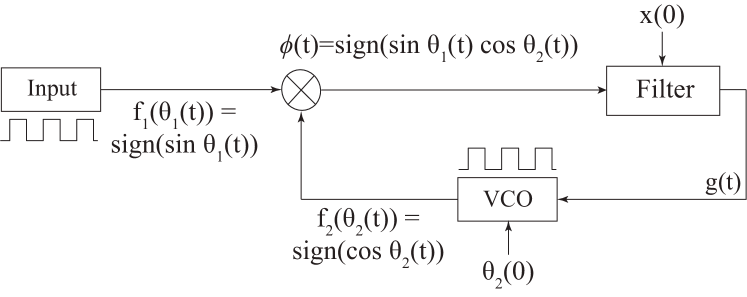
Consider a physical model of classical PLL in the signals space (see Fig. 1
Figure 1: Model of PLL with impulse signals in the signals space.
This model contains the following blocks: a reference oscillator (Input), a voltage-controlled oscillator (VCO), a filter (Filter), and an analog multiplier as a phase detector (PD).
The signals sign ( sin θ 1 ( t ) ) sign subscript 𝜃 1 𝑡 \operatorname{sign}\left(\sin\theta_{1}(t)\right) sign ( cos θ 2 ( t ) ) sign subscript 𝜃 2 𝑡 \operatorname{sign}\left(\cos\theta_{2}(t)\right) θ 2 ( 0 ) subscript 𝜃 2 0 \theta_{2}(0) ϕ ( t ) = sign ( sin θ 1 ( t ) cos θ 2 ( t ) ) italic-ϕ 𝑡 sign subscript 𝜃 1 𝑡 subscript 𝜃 2 𝑡 \phi(t)=\operatorname{sign}\left(\sin\theta_{1}(t)\cos\theta_{2}(t)\right) x ( 0 ) 𝑥 0 x(0) g ( t ) 𝑔 𝑡 g(t)
The equations describing the model of PLL-based circuits in the signals space are difficult for the study, since that equations are nonautonomous (see, e.g., (Kudrewicz and Wasowicz, 2007 ) ). By contrast, the equations of model in the signal’s phase space are autonomous
(Gardner, 1966 ; Shakhgil’dyan and Lyakhovkin, 1966 ; Viterbi, 1966 ) , what simplifies the study of PLL-based circuits.
The application of averaging methods (Mitropolsky and Bogolubov, 1961 ; Samoilenko and Petryshyn, 2004 ) allows one to reduce the model of PLL-based circuits in the signals space to the model in
the signal’s phase space
(see, e.g., (Leonov et al., 2012 ; Leonov and Kuznetsov, 2014 ; Leonov et al., 2015a ; Kuznetsov et al., 2015b , a ; Best et al., 2015 ) .
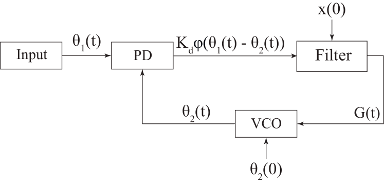
Figure 2: Model of the classical PLL in the signal’s phase space.
The main difference between the physical model (Fig. 1 2
K d φ ( θ 1 ( t ) − θ 2 ( t ) ) . subscript 𝐾 𝑑 𝜑 subscript 𝜃 1 𝑡 subscript 𝜃 2 𝑡 K_{d}\varphi(\theta_{1}(t)-\theta_{2}(t)).
The maximum absolute value of PD output K d > 0 subscript 𝐾 𝑑 0 K_{d}>0 (Best, 2007 ; Goldman, 2007 ) ). The periodic function φ ( θ Δ ( t ) ) 𝜑 subscript 𝜃 Δ 𝑡 \varphi(\theta_{\Delta}(t)) θ 1 ( t ) − θ 2 ( t ) subscript 𝜃 1 𝑡 subscript 𝜃 2 𝑡 \theta_{1}(t)-\theta_{2}(t) θ Δ ( t ) subscript 𝜃 Δ 𝑡 \theta_{\Delta}(t) f 1 ( θ 1 ) subscript 𝑓 1 subscript 𝜃 1 f_{1}(\theta_{1}) f 2 ( θ 2 ) subscript 𝑓 2 subscript 𝜃 2 f_{2}(\theta_{2}) (Viterbi, 1966 ; Gardner, 1966 ; Leonov et al., 2012 ) ):
K d = 1 ; subscript 𝐾 𝑑 1 \displaystyle K_{d}=1;
φ ( θ Δ ( t ) ) = { 2 π θ Δ ( t ) , if − π 2 ≤ θ Δ ( t ) ≤ π 2 , − 2 π θ Δ ( t ) + 2 , if π 2 ≤ θ Δ ( t ) ≤ 3 π 2 . 𝜑 subscript 𝜃 Δ 𝑡 cases 2 𝜋 subscript 𝜃 Δ 𝑡 if − π 2 ≤ θ Δ ( t ) ≤ π 2 , 2 𝜋 subscript 𝜃 Δ 𝑡 2 if π 2 ≤ θ Δ ( t ) ≤ 3 π 2 \displaystyle\varphi(\theta_{\Delta}(t))=\begin{cases}\frac{2}{\pi}\theta_{\Delta}(t),&\text{if $-\frac{\pi}{2}\leq\theta_{\Delta}(t)\leq\frac{\pi}{2}$,}\\
-\frac{2}{\pi}\theta_{\Delta}(t)+2,&\text{if $\frac{\pi}{2}\leq\theta_{\Delta}(t)\leq\frac{3\pi}{2}$}.\end{cases} (1)
Let us describe a model of classical PLL with impulse signals in the signal’s phase
space (see Fig. 2 θ 1 ( t ) subscript 𝜃 1 𝑡 \theta_{1}(t) θ 2 ( t ) subscript 𝜃 2 𝑡 \theta_{2}(t)
θ ˙ 1 ( t ) = ω 1 . subscript ˙ 𝜃 1 𝑡 subscript 𝜔 1 \dot{\theta}_{1}(t)=\omega_{1}. (2)
The phases θ 1 ( t ) subscript 𝜃 1 𝑡 \theta_{1}(t) θ 2 ( t ) subscript 𝜃 2 𝑡 \theta_{2}(t) (Baker, 2011 ) ) with transfer function
W ( s ) = 1 + τ 2 s τ 1 s 𝑊 𝑠 1 subscript 𝜏 2 𝑠 subscript 𝜏 1 𝑠 W(s)=\frac{1+\tau_{2}s}{\tau_{1}s} τ 1 > 0 subscript 𝜏 1 0 \tau_{1}\leavevmode\nobreak\ >\leavevmode\nobreak\ 0 τ 2 > 0 subscript 𝜏 2 0 \tau_{2}\leavevmode\nobreak\ >\leavevmode\nobreak\ 0
{ x ˙ ( t ) = K d φ ( θ Δ ( t ) ) , G ( t ) = 1 τ 1 x ( t ) + τ 2 τ 1 K d φ ( θ Δ ( t ) ) , cases ˙ 𝑥 𝑡 subscript 𝐾 𝑑 𝜑 subscript 𝜃 Δ 𝑡 otherwise 𝐺 𝑡 1 subscript 𝜏 1 𝑥 𝑡 subscript 𝜏 2 subscript 𝜏 1 subscript 𝐾 𝑑 𝜑 subscript 𝜃 Δ 𝑡 otherwise \begin{cases}\dot{x}(t)=K_{d}\varphi(\theta_{\Delta}(t)),\\
G(t)=\frac{1}{\tau_{1}}x(t)+\frac{\tau_{2}}{\tau_{1}}K_{d}\varphi(\theta_{\Delta}(t)),\end{cases} (3)
where x ( t ) 𝑥 𝑡 x(t)
The output of Filter G ( t ) 𝐺 𝑡 G(t)
θ ˙ 2 ( t ) = ω 2 free + K v G ( t ) , subscript ˙ 𝜃 2 𝑡 superscript subscript 𝜔 2 free subscript 𝐾 𝑣 𝐺 𝑡 \dot{\theta}_{2}(t)=\omega_{2}^{\rm free}+K_{v}G(t), (4)
where ω 2 free superscript subscript 𝜔 2 free \omega_{2}^{\rm free} K v > 0 subscript 𝐾 𝑣 0 K_{v}>0
Relations (2 3 4
{ x ˙ = K d φ ( θ Δ ) , θ ˙ Δ = ω 1 − ω 2 free − K v τ 1 ( x + τ 2 K d φ ( θ Δ ) ) . cases ˙ 𝑥 subscript 𝐾 𝑑 𝜑 subscript 𝜃 Δ otherwise subscript ˙ 𝜃 Δ subscript 𝜔 1 superscript subscript 𝜔 2 free subscript 𝐾 𝑣 subscript 𝜏 1 𝑥 subscript 𝜏 2 subscript 𝐾 𝑑 𝜑 subscript 𝜃 Δ otherwise \begin{cases}\dot{x}=K_{d}\varphi(\theta_{\Delta}),\\
\dot{\theta}_{\Delta}=\omega_{1}-\omega_{2}^{\rm free}-\frac{K_{v}}{\tau_{1}}\left(x+\tau_{2}K_{d}\varphi(\theta_{\Delta})\right).\end{cases} (5)
Denote the difference of the reference frequency and the VCO free-running frequency ω 1 − ω 2 free subscript 𝜔 1 superscript subscript 𝜔 2 free \omega_{1}-\omega_{2}^{\rm free} ω Δ free superscript subscript 𝜔 Δ free \omega_{\Delta}^{\rm free} x → K d x → 𝑥 subscript 𝐾 𝑑 𝑥 x\rightarrow K_{d}x
{ x ˙ = φ ( θ Δ ) , θ ˙ Δ = ω Δ free − K 0 τ 1 ( x + τ 2 φ ( θ Δ ) ) , cases ˙ 𝑥 𝜑 subscript 𝜃 Δ otherwise subscript ˙ 𝜃 Δ superscript subscript 𝜔 Δ free subscript 𝐾 0 subscript 𝜏 1 𝑥 subscript 𝜏 2 𝜑 subscript 𝜃 Δ otherwise \begin{cases}\dot{x}=\varphi(\theta_{\Delta}),\\
\dot{\theta}_{\Delta}=\omega_{\Delta}^{\rm free}-\frac{K_{0}}{\tau_{1}}\left(x+\tau_{2}\varphi(\theta_{\Delta})\right),\end{cases} (6)
where K 0 = K v K d subscript 𝐾 0 subscript 𝐾 𝑣 subscript 𝐾 𝑑 K_{0}=K_{v}K_{d} 6
By the transformation
( ω Δ free , x , θ Δ ) → ( − ω Δ free , − x , − θ Δ ) , → superscript subscript 𝜔 Δ free 𝑥 subscript 𝜃 Δ superscript subscript 𝜔 Δ free 𝑥 subscript 𝜃 Δ \left(\omega_{\Delta}^{\rm free},x,\theta_{\Delta}\right)\rightarrow\left(-\omega_{\Delta}^{\rm free},-x,-\theta_{\Delta}\right),
(6 1
| ω Δ free | = | ω 1 − ω 2 free | superscript subscript 𝜔 Δ free subscript 𝜔 1 superscript subscript 𝜔 2 free \left|\omega_{\Delta}^{\rm free}\right|=\left|\omega_{1}-\omega_{2}^{\rm free}\right|
and consider (6 ω Δ free > 0 superscript subscript 𝜔 Δ free 0 \omega_{\Delta}^{\rm free}>0
The PLL state for which the VCO frequency is adjusted to the reference frequency of Input is called a locked state.
The locked states of the PLL correspond to the locally asymptotically stable equilibria of (6
{ φ ( θ e q ) = 0 , ω Δ free − K 0 τ 1 x e q = 0 . cases 𝜑 subscript 𝜃 𝑒 𝑞 0 otherwise superscript subscript 𝜔 Δ free subscript 𝐾 0 subscript 𝜏 1 subscript 𝑥 𝑒 𝑞 0 otherwise \begin{cases}\varphi(\theta_{eq})=0,\\
\omega_{\Delta}^{\rm free}-\frac{K_{0}}{\tau_{1}}x_{eq}=0.\end{cases}
Since (6 2 π 2 𝜋 2\pi θ Δ subscript 𝜃 Δ \theta_{\Delta} 6 2 π 2 𝜋 2\pi θ Δ subscript 𝜃 Δ \theta_{\Delta} θ Δ ∈ ( − π , π ] subscript 𝜃 Δ 𝜋 𝜋 \theta_{\Delta}\in\left(-\pi,\pi\right] θ Δ ∈ ( − π , π ] subscript 𝜃 Δ 𝜋 𝜋 \theta_{\Delta}\in\left(-\pi,\pi\right]
( θ e q s , x e q ( ω Δ free ) ) = ( 0 , ω Δ free τ 1 K 0 ) and ( θ e q u , x e q ( ω Δ free ) ) = ( π , ω Δ free τ 1 K 0 ) . superscript subscript 𝜃 𝑒 𝑞 𝑠 subscript 𝑥 𝑒 𝑞 superscript subscript 𝜔 Δ free 0 superscript subscript 𝜔 Δ free subscript 𝜏 1 subscript 𝐾 0 and superscript subscript 𝜃 𝑒 𝑞 𝑢 subscript 𝑥 𝑒 𝑞 superscript subscript 𝜔 Δ free 𝜋 superscript subscript 𝜔 Δ free subscript 𝜏 1 subscript 𝐾 0 \left(\theta_{eq}^{s},x_{eq}(\omega_{\Delta}^{\rm free})\right)=(0,\frac{\omega_{\Delta}^{\rm free}\tau_{1}}{K_{0}})\text{ and }\left(\theta_{eq}^{u},x_{eq}(\omega_{\Delta}^{\rm free})\right)=(\pi,\frac{\omega_{\Delta}^{\rm free}\tau_{1}}{K_{0}}).
As is shown below (see A
( θ e q s + 2 π k , x e q ( ω Δ free ) ) = ( 2 π k , ω Δ free τ 1 K 0 ) superscript subscript 𝜃 𝑒 𝑞 𝑠 2 𝜋 𝑘 subscript 𝑥 𝑒 𝑞 superscript subscript 𝜔 Δ free 2 𝜋 𝑘 superscript subscript 𝜔 Δ free subscript 𝜏 1 subscript 𝐾 0 \left(\theta_{eq}^{s}+2\pi k,x_{eq}(\omega_{\Delta}^{\rm free})\right)=\left(2\pi k,\frac{\omega_{\Delta}^{\rm free}\tau_{1}}{K_{0}}\right)
are locally asymptotically stable. Hence, the locked states of (6 ( θ e q s , x e q ( ω Δ free ) ) superscript subscript 𝜃 𝑒 𝑞 𝑠 subscript 𝑥 𝑒 𝑞 superscript subscript 𝜔 Δ free \left(\theta_{eq}^{s},x_{eq}(\omega_{\Delta}^{\rm free})\right)
( θ e q u + 2 π k , x e q ( ω Δ free ) ) = ( π + 2 π k , ω Δ free τ 1 K 0 ) superscript subscript 𝜃 𝑒 𝑞 𝑢 2 𝜋 𝑘 subscript 𝑥 𝑒 𝑞 superscript subscript 𝜔 Δ free 𝜋 2 𝜋 𝑘 superscript subscript 𝜔 Δ free subscript 𝜏 1 subscript 𝐾 0 \left(\theta_{eq}^{u}+2\pi k,x_{eq}(\omega_{\Delta}^{\rm free})\right)=\left(\pi+2\pi k,\frac{\omega_{\Delta}^{\rm free}\tau_{1}}{K_{0}}\right)
are saddle equilibria (see A
2 The lock-in range
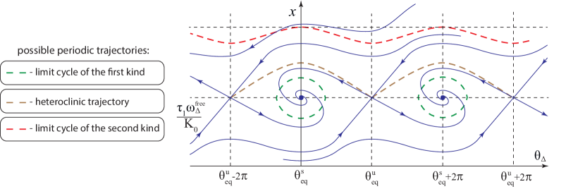
The model of classical PLL with impulse signals and active PI filter in the signal’s phase space is globally asymptotically stable (see, e.g., (Gubar’, 1961 ; Leonov and Aleksandrov, 2015 ) ). The PLL achieves locked state for any initial VCO phase θ 2 ( 0 ) subscript 𝜃 2 0 \theta_{2}(0) x ( 0 ) 𝑥 0 x(0) 6 3
Figure 3: Possible periodic trajectories on the phase plane of (6
However, the phase error θ Δ subscript 𝜃 Δ \theta_{\Delta} θ Δ subscript 𝜃 Δ \theta_{\Delta} (Gardner, 1966 ) :
“If, for some reason, the frequency difference between input and VCO is less than the loop bandwidth, the loop will lock up almost instantaneously without slipping cycles. The maximum frequency difference for which this fast acquisition is possible is called the lock-in frequency ”.
The lock-in range concept is widely used in engineering literature on the PLL-based circuits study (see, e.g., (Stensby, 1997 ; Kihara et al., 2002 ; Kroupa, 2003 ; Gardner, 2005 ; Best, 2007 ) ).
It is said that a cycle slipping occurs if (see, e.g., (Ascheid and Meyr, 1982 ; Ershova and Leonov, 1983 ; Smirnova et al., 2014 ) )
lim sup t → + ∞ | θ Δ ( 0 ) − θ Δ ( t ) | ≥ 2 π . subscript limit-supremum → 𝑡 subscript 𝜃 Δ 0 subscript 𝜃 Δ 𝑡 2 𝜋 \displaystyle\limsup_{t\rightarrow+\infty}\left|\theta_{\Delta}(0)-\theta_{\Delta}(t)\right|\geq 2\pi.
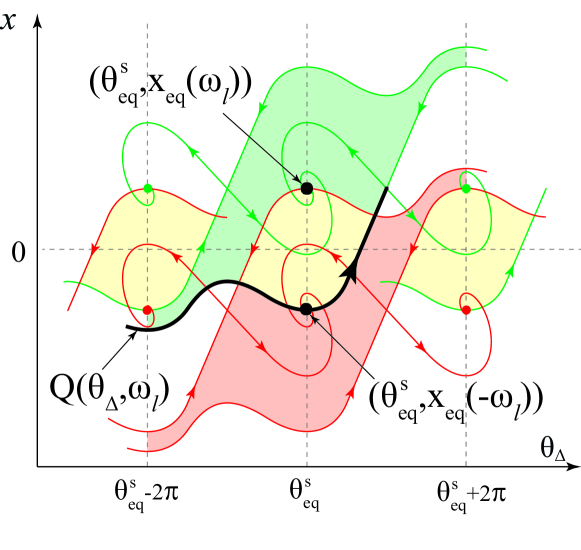
Figure 4: The lock-in domain and cycle slipping.
However, in general, even for zero frequency deviation (ω Δ free = 0 superscript subscript 𝜔 Δ free 0 \omega_{\Delta}^{\text{free}}=0 x ( 0 ) 𝑥 0 x(0) “There is no natural way to define exactly any unique lock-in frequency” and “despite its vague reality, lock-in range is a useful concept” (Gardner, 1979 ) .
To overcome the stated problem, in (Kuznetsov et al., 2015c ; Leonov et al., 2015b ) the rigorous mathematical definition of a lock-in range is suggested:
Definition 1
( Kuznetsov et al., 2015c ; Leonov et al., 2015b )
The lock-in range of model (6 [ 0 , ω l ) 0 subscript 𝜔 𝑙 \left[0,\omega_{l}\right) | ω Δ free | ∈ [ 0 , ω l ) superscript subscript 𝜔 Δ free 0 subscript 𝜔 𝑙 \left|\omega_{\Delta}^{\rm free}\right|\in\left[0,\omega_{l}\right) 6
D lock − in ( ( − ω l , ω l ) ) = ⋂ | ω Δ free | < ω l D lock − in ( ω Δ free ) subscript 𝐷 lock in subscript 𝜔 𝑙 subscript 𝜔 𝑙 superscript subscript 𝜔 Δ free subscript 𝜔 𝑙 subscript 𝐷 lock in superscript subscript 𝜔 Δ free D_{\rm lock-in}\left((-\omega_{l},\omega_{l})\right)=\underset{\left|\omega_{\Delta}^{\rm free}\right|<\omega_{l}}{\bigcap}D_{\rm lock-in}(\omega_{\Delta}^{\rm free})
contains all corresponding equilibria ( θ e q s , x e q ( ω Δ free ) ) . subscript superscript 𝜃 𝑠 𝑒 𝑞 subscript 𝑥 𝑒 𝑞 superscript subscript 𝜔 Δ free \left(\theta^{s}_{eq},x_{eq}(\omega_{\Delta}^{\rm free})\right).
For model (6 ⋂ | ω Δ free | < ω l D lock − in ( ω Δ free ) superscript subscript 𝜔 Δ free subscript 𝜔 𝑙 subscript 𝐷 lock in superscript subscript 𝜔 Δ free \underset{\left|\omega_{\Delta}^{\rm free}\right|<\omega_{l}}{\bigcap}D_{\rm lock-in}(\omega_{\Delta}^{\rm free}) ( θ e q u , x e q ( ω Δ free ) ) subscript superscript 𝜃 𝑢 𝑒 𝑞 subscript 𝑥 𝑒 𝑞 superscript subscript 𝜔 Δ free \left(\theta^{u}_{eq},x_{eq}(\omega_{\Delta}^{\rm free})\right) θ Δ = θ e q s ± 2 π subscript 𝜃 Δ plus-or-minus subscript superscript 𝜃 𝑠 𝑒 𝑞 2 𝜋 \theta_{\Delta}=\theta^{s}_{eq}\pm 2\pi 5
3 Phase plane analysis for the lock-in range estimation
Consider an approach to the lock-in range computation of (6 6 Q ( θ Δ , ω Δ free ) 𝑄 subscript 𝜃 Δ superscript subscript 𝜔 Δ free Q(\theta_{\Delta},\omega_{\Delta}^{\rm free}) ( θ e q u , x e q ( ω Δ free ) ) = ( π , ω Δ free τ 1 K 0 ) superscript subscript 𝜃 𝑒 𝑞 𝑢 subscript 𝑥 𝑒 𝑞 superscript subscript 𝜔 Δ free 𝜋 superscript subscript 𝜔 Δ free subscript 𝜏 1 subscript 𝐾 0 \left(\theta_{eq}^{u},x_{eq}(\omega_{\Delta}^{\rm free})\right)=\left(\pi,\frac{\omega_{\Delta}^{\rm free}\tau_{1}}{K_{0}}\right) t → + ∞ → 𝑡 t\rightarrow+\infty ω Δ free superscript subscript 𝜔 Δ free \omega_{\Delta}^{\rm free} x → x + ω Δ free τ 1 K 0 → 𝑥 𝑥 superscript subscript 𝜔 Δ free subscript 𝜏 1 subscript 𝐾 0 x\rightarrow x+\frac{\omega_{\Delta}^{\rm free}\tau_{1}}{K_{0}} 6 ω Δ free = ω l superscript subscript 𝜔 Δ free subscript 𝜔 𝑙 \omega_{\Delta}^{\rm free}=\omega_{l} ω l subscript 𝜔 𝑙 \omega_{l} 5
x e q ( − ω l ) = Q ( θ e q s , ω l ) . subscript 𝑥 𝑒 𝑞 subscript 𝜔 𝑙 𝑄 subscript superscript 𝜃 𝑠 𝑒 𝑞 subscript 𝜔 𝑙 x_{eq}(-\omega_{l})=Q(\theta^{s}_{eq},\omega_{l}). (7)
By (7 ω l subscript 𝜔 𝑙 \omega_{l}
− ω l K 0 / τ 1 = ω l K 0 / τ 1 + Q ( θ e q s , 0 ) . subscript 𝜔 𝑙 subscript 𝐾 0 subscript 𝜏 1 subscript 𝜔 𝑙 subscript 𝐾 0 subscript 𝜏 1 𝑄 subscript superscript 𝜃 𝑠 𝑒 𝑞 0 \displaystyle-\frac{\omega_{l}}{K_{0}/\tau_{1}}=\frac{\omega_{l}}{K_{0}/\tau_{1}}+Q(\theta^{s}_{eq},0).
ω l = − K 0 Q ( θ e q s , 0 ) 2 τ 1 , subscript 𝜔 𝑙 subscript 𝐾 0 𝑄 subscript superscript 𝜃 𝑠 𝑒 𝑞 0 2 subscript 𝜏 1 \displaystyle\omega_{l}=-\frac{K_{0}Q(\theta^{s}_{eq},0)}{2\tau_{1}}, (8)
Figure 5: The lock-in domain of (6 | ω Δ free | = ω l superscript subscript 𝜔 Δ free subscript 𝜔 𝑙 \left|\omega_{\Delta}^{\rm free}\right|=\omega_{l}
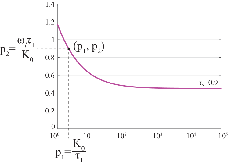
Numerical simulations are used to compute the lock-in range of (6 8 Q ( θ Δ , 0 ) 𝑄 subscript 𝜃 Δ 0 Q(\theta_{\Delta},0) ω l subscript 𝜔 𝑙 \omega_{l} 6 6 K 0 τ 1 subscript 𝐾 0 subscript 𝜏 1 \frac{K_{0}}{\tau_{1}} τ 2 subscript 𝜏 2 \tau_{2} 6 K 0 τ 1 subscript 𝐾 0 subscript 𝜏 1 \frac{K_{0}}{\tau_{1}} τ 2 subscript 𝜏 2 \tau_{2} K 0 τ 1 subscript 𝐾 0 subscript 𝜏 1 \frac{K_{0}}{\tau_{1}} ω l subscript 𝜔 𝑙 \omega_{l} K 0 τ 1 subscript 𝐾 0 subscript 𝜏 1 \frac{K_{0}}{\tau_{1}} ω l τ 1 K 0 subscript 𝜔 𝑙 subscript 𝜏 1 subscript 𝐾 0 \frac{\omega_{l}\tau_{1}}{K_{0}} K 0 τ 1 subscript 𝐾 0 subscript 𝜏 1 \frac{K_{0}}{\tau_{1}} 6 ω Δ free τ 1 K 0 superscript subscript 𝜔 Δ free subscript 𝜏 1 subscript 𝐾 0 \frac{\omega_{\Delta}^{\rm free}\tau_{1}}{K_{0}}
To obtain the lock-in frequency ω l subscript 𝜔 𝑙 \omega_{l} τ 1 subscript 𝜏 1 \tau_{1} τ 2 subscript 𝜏 2 \tau_{2} K 0 subscript 𝐾 0 K_{0} 6 τ 2 subscript 𝜏 2 \tau_{2} K 0 τ 1 subscript 𝐾 0 subscript 𝜏 1 \frac{K_{0}}{\tau_{1}} K 0 τ 1 subscript 𝐾 0 subscript 𝜏 1 \frac{K_{0}}{\tau_{1}}
Figure 6: Diagram for the lock-in frequency ω l subscript 𝜔 𝑙 \omega_{l}
Consider an analytical approach to the exact lock-in range computation.
Main stages of computation are presented in Subsection 3.1
3.1 Analytical approach to the lock-in range computation
Consider a system
{ θ ˙ Δ ( t ) = y ( t ) , y ˙ ( t ) = − K 0 τ 2 τ 1 φ ˙ ( θ Δ ( t ) ) y ( t ) − K 0 τ 1 φ ( θ Δ ( t ) ) , cases subscript ˙ 𝜃 Δ 𝑡 𝑦 𝑡 otherwise ˙ 𝑦 𝑡 subscript 𝐾 0 subscript 𝜏 2 subscript 𝜏 1 ˙ 𝜑 subscript 𝜃 Δ 𝑡 𝑦 𝑡 subscript 𝐾 0 subscript 𝜏 1 𝜑 subscript 𝜃 Δ 𝑡 otherwise \begin{cases}\dot{\theta}_{\Delta}(t)=y(t),\\
\dot{y}(t)=-\frac{K_{0}\tau_{2}}{\tau_{1}}\dot{\varphi}(\theta_{\Delta}(t))y(t)-\frac{K_{0}}{\tau_{1}}\varphi(\theta_{\Delta}(t)),\end{cases} (9)
where y ( t ) = ω Δ free − K 0 τ 1 ( x ( t ) + τ 2 φ ( θ Δ ( t ) ) ) 𝑦 𝑡 superscript subscript 𝜔 Δ free subscript 𝐾 0 subscript 𝜏 1 𝑥 𝑡 subscript 𝜏 2 𝜑 subscript 𝜃 Δ 𝑡 y(t)=\omega_{\Delta}^{\rm free}-\frac{K_{0}}{\tau_{1}}\left(x(t)+\tau_{2}\varphi(\theta_{\Delta}(t))\right) 9 6 ω Δ free superscript subscript 𝜔 Δ free \omega_{\Delta}^{\rm free} ( θ e q , y e q ) subscript 𝜃 𝑒 𝑞 subscript 𝑦 𝑒 𝑞 \left(\theta_{eq},y_{eq}\right) 9 ( θ e q , x e q ) subscript 𝜃 𝑒 𝑞 subscript 𝑥 𝑒 𝑞 \left(\theta_{eq},x_{eq}\right) 6
( θ e q , y e q ) = ( θ e q , ω Δ free − K 0 b x e q ) . subscript 𝜃 𝑒 𝑞 subscript 𝑦 𝑒 𝑞 subscript 𝜃 𝑒 𝑞 superscript subscript 𝜔 Δ free subscript 𝐾 0 𝑏 subscript 𝑥 𝑒 𝑞 \left(\theta_{eq},y_{eq}\right)=\left(\theta_{eq},\omega_{\Delta}^{\rm free}-K_{0}bx_{eq}\right).
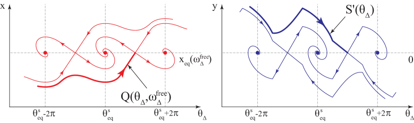
The separatrix Q ( θ Δ , ω Δ free ) 𝑄 subscript 𝜃 Δ superscript subscript 𝜔 Δ free Q(\theta_{\Delta},\omega_{\Delta}^{\rm free}) 8 S ′ ( θ Δ ) superscript 𝑆 ′ subscript 𝜃 Δ S^{\prime}(\theta_{\Delta}) 9 7
Q ( θ e q s , ω Δ free ) = τ 1 K 0 ( ω Δ free − S ′ ( θ e q s ) ) 𝑄 subscript superscript 𝜃 𝑠 𝑒 𝑞 superscript subscript 𝜔 Δ free subscript 𝜏 1 subscript 𝐾 0 superscript subscript 𝜔 Δ free superscript 𝑆 ′ subscript superscript 𝜃 𝑠 𝑒 𝑞 Q(\theta^{s}_{eq},\omega_{\Delta}^{\rm free})=\frac{\tau_{1}}{K_{0}}\left(\omega_{\Delta}^{\rm free}-S^{\prime}(\theta^{s}_{eq})\right)
is valid.
Figure 7: Phase plane portraits of (6 9
Relation (8
ω l = 1 2 S ′ ( θ e q s ) . subscript 𝜔 𝑙 1 2 superscript 𝑆 ′ subscript superscript 𝜃 𝑠 𝑒 𝑞 \omega_{l}=\frac{1}{2}S^{\prime}(\theta^{s}_{eq}). (10)
The computation of the separatrix S ′ ( θ Δ ) superscript 𝑆 ′ subscript 𝜃 Δ S^{\prime}(\theta_{\Delta}) 1 1 1 S ′ ( θ Δ ) superscript 𝑆 ′ subscript 𝜃 Δ S^{\prime}(\theta_{\Delta}) ( π 2 , π ) 𝜋 2 𝜋 \left(\frac{\pi}{2},\pi\right) φ ( θ Δ ) 𝜑 subscript 𝜃 Δ \varphi(\theta_{\Delta}) S ′ ( π 2 ) superscript 𝑆 ′ 𝜋 2 S^{\prime}(\frac{\pi}{2}) S ′ ( θ Δ ) superscript 𝑆 ′ subscript 𝜃 Δ S^{\prime}(\theta_{\Delta}) 9 ( − π 2 , π 2 ) 𝜋 2 𝜋 2 \left(-\frac{\pi}{2},\frac{\pi}{2}\right) ( θ e q s , 0 ) subscript superscript 𝜃 𝑠 𝑒 𝑞 0 \left(\theta^{s}_{eq},0\right) S ′ ( π 2 ) superscript 𝑆 ′ 𝜋 2 S^{\prime}(\frac{\pi}{2}) S ′ ( θ e q s ) superscript 𝑆 ′ subscript superscript 𝜃 𝑠 𝑒 𝑞 S^{\prime}(\theta^{s}_{eq})
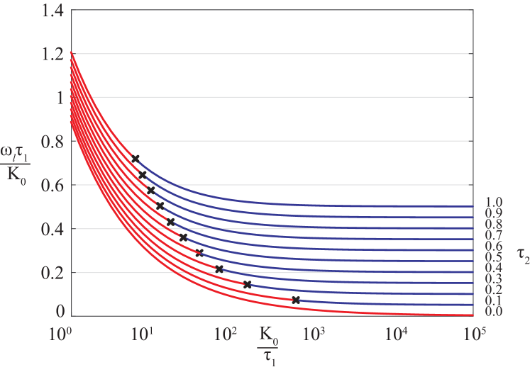
The obtained analytical results are illustrated in Fig. 8 8
Figure 8: Diagram for the lock-in frequency ω l subscript 𝜔 𝑙 \omega_{l}
The formulae for three possible cases are given below (redefinitions a = τ 2 τ 1 𝑎 subscript 𝜏 2 subscript 𝜏 1 a=\frac{\tau_{2}}{\tau_{1}} b = 1 τ 1 𝑏 1 subscript 𝜏 1 b=\frac{1}{\tau_{1}} A. ( a K 0 ) 2 − 2 b K 0 π > 0 superscript 𝑎 subscript 𝐾 0 2 2 𝑏 subscript 𝐾 0 𝜋 0 (aK_{0})^{2}-2bK_{0}\pi>0
ω l = 1 π c 1 ( a K 0 ) 2 − 2 b K 0 π ( − c 2 c 1 ) ( 1 2 − a K 0 2 ( a K 0 ) 2 − 2 b K 0 π ) , subscript 𝜔 𝑙 1 𝜋 subscript 𝑐 1 superscript 𝑎 subscript 𝐾 0 2 2 𝑏 subscript 𝐾 0 𝜋 superscript subscript 𝑐 2 subscript 𝑐 1 1 2 𝑎 subscript 𝐾 0 2 superscript 𝑎 subscript 𝐾 0 2 2 𝑏 subscript 𝐾 0 𝜋 \displaystyle\omega_{l}=\displaystyle\frac{1}{\pi}c_{1}\sqrt{(aK_{0})^{2}-2bK_{0}\pi}\hskip 2.84544pt\left(-\frac{c_{2}}{c_{1}}\right)^{\left(\displaystyle\frac{1}{2}-\frac{aK_{0}}{\displaystyle 2\sqrt{(aK_{0})^{2}-2bK_{0}\pi}}\right)}, (11)
where c 1 = π 4 ( ( a K 0 ) 2 + 2 b K 0 π ( a K 0 ) 2 − 2 b K 0 π + 1 ) , c 2 = π 4 ( 1 − ( a K 0 ) 2 + 2 b K 0 π ( a K 0 ) 2 − 2 b K 0 π ) . formulae-sequence where subscript 𝑐 1 𝜋 4 superscript 𝑎 subscript 𝐾 0 2 2 𝑏 subscript 𝐾 0 𝜋 superscript 𝑎 subscript 𝐾 0 2 2 𝑏 subscript 𝐾 0 𝜋 1 subscript 𝑐 2 𝜋 4 1 superscript 𝑎 subscript 𝐾 0 2 2 𝑏 subscript 𝐾 0 𝜋 superscript 𝑎 subscript 𝐾 0 2 2 𝑏 subscript 𝐾 0 𝜋 \displaystyle\text{where }c_{1}=\frac{\pi}{4}\left(\displaystyle\frac{\sqrt{(aK_{0})^{2}+2bK_{0}\pi}}{\sqrt{(aK_{0})^{2}-2bK_{0}\pi}}+1\right),c_{2}=\frac{\pi}{4}\left(1-\displaystyle\frac{\sqrt{(aK_{0})^{2}+2bK_{0}\pi}}{\sqrt{(aK_{0})^{2}-2bK_{0}\pi}}\right).
B. ( a K 0 ) 2 − 2 b K 0 π = 0 superscript 𝑎 subscript 𝐾 0 2 2 𝑏 subscript 𝐾 0 𝜋 0 (aK_{0})^{2}-2bK_{0}\pi=0
ω l = 1 2 c 2 e ( a K 0 2 c 2 ) , where c 2 = ( a K 0 ) 2 + 2 b K 0 π 2 . formulae-sequence subscript 𝜔 𝑙 1 2 subscript 𝑐 2 superscript 𝑒 𝑎 subscript 𝐾 0 2 subscript 𝑐 2 where subscript 𝑐 2 superscript 𝑎 subscript 𝐾 0 2 2 𝑏 subscript 𝐾 0 𝜋 2 \displaystyle\omega_{l}=\frac{1}{2}c_{2}\hskip 2.84544pte^{\left(\displaystyle\frac{aK_{0}}{2c_{2}}\right)},\text{where }c_{2}=\displaystyle\frac{\sqrt{(aK_{0})^{2}+2bK_{0}\pi}}{2}. (12)
C. ( a K 0 ) 2 − 2 b K 0 π < 0 superscript 𝑎 subscript 𝐾 0 2 2 𝑏 subscript 𝐾 0 𝜋 0 (aK_{0})^{2}-2bK_{0}\pi<0
ω l = − a K 0 e t 0 Re λ 1 s 2 π ( c 1 cos ( t 0 Im λ 1 s ) + c 2 sin ( t 0 Im λ 1 s ) ) + subscript 𝜔 𝑙 limit-from 𝑎 subscript 𝐾 0 superscript 𝑒 subscript 𝑡 0 Re subscript superscript 𝜆 𝑠 1 2 𝜋 subscript 𝑐 1 subscript 𝑡 0 Im subscript superscript 𝜆 𝑠 1 subscript 𝑐 2 subscript 𝑡 0 Im subscript superscript 𝜆 𝑠 1 \displaystyle\omega_{l}=\displaystyle-\frac{aK_{0}\hskip 2.84544pte^{\displaystyle t_{0}\operatorname{Re}\lambda^{s}_{1}}}{2\pi}\left(c_{1}\cos\left(t_{0}\operatorname{Im}\lambda^{s}_{1}\right)+c_{2}\sin\left(t_{0}\operatorname{Im}\lambda^{s}_{1}\right)\right)+
+ e t 0 Re λ 1 s 2 b K 0 π − ( a K 0 ) 2 2 π ( c 2 cos ( t 0 Im λ 1 s ) − c 1 sin ( t 0 Im λ 1 s ) ) , superscript 𝑒 subscript 𝑡 0 Re subscript superscript 𝜆 𝑠 1 2 𝑏 subscript 𝐾 0 𝜋 superscript 𝑎 subscript 𝐾 0 2 2 𝜋 subscript 𝑐 2 subscript 𝑡 0 Im subscript superscript 𝜆 𝑠 1 subscript 𝑐 1 subscript 𝑡 0 Im subscript superscript 𝜆 𝑠 1 \displaystyle+\displaystyle\frac{e^{\displaystyle t_{0}\operatorname{Re}\lambda^{s}_{1}}\sqrt{2bK_{0}\pi-(aK_{0})^{2}}}{2\pi}\left(c_{2}\cos\left(t_{0}\operatorname{Im}\lambda^{s}_{1}\right)-c_{1}\sin\left(t_{0}\operatorname{Im}\lambda^{s}_{1}\right)\right), (13)
where t 0 = arctg ( − c 1 c 2 ) Im λ 1 s , c 1 = π 2 , c 2 = π ( a K 0 ) 2 + 4 b K 0 ( π − 1 k ) 2 2 b K 0 π − ( a K 0 ) 2 , formulae-sequence where subscript 𝑡 0 arctg subscript 𝑐 1 subscript 𝑐 2 Im subscript superscript 𝜆 𝑠 1 formulae-sequence subscript 𝑐 1 𝜋 2 subscript 𝑐 2 𝜋 superscript 𝑎 subscript 𝐾 0 2 4 𝑏 subscript 𝐾 0 𝜋 1 𝑘 2 2 𝑏 subscript 𝐾 0 𝜋 superscript 𝑎 subscript 𝐾 0 2 \displaystyle\text{where }t_{0}=\frac{\operatorname{arctg}\left(\displaystyle-\frac{c_{1}}{c_{2}}\right)}{\operatorname{Im}\lambda^{s}_{1}},c_{1}=\displaystyle\frac{\pi}{2},\hskip 5.69046ptc_{2}=\displaystyle\frac{\pi\sqrt{(aK_{0})^{2}+4{b}K_{0}({\pi}-\frac{1}{k})}}{\displaystyle 2\sqrt{2bK_{0}\pi-(aK_{0})^{2}}},
λ 1 s = − a K 0 + i 2 b K 0 π − ( a K 0 ) 2 π . subscript superscript 𝜆 𝑠 1 𝑎 subscript 𝐾 0 𝑖 2 𝑏 subscript 𝐾 0 𝜋 superscript 𝑎 subscript 𝐾 0 2 𝜋 \displaystyle\lambda^{s}_{1}=\displaystyle\frac{-aK_{0}+i\sqrt{2bK_{0}\pi-(aK_{0})^{2}}}{\pi}.
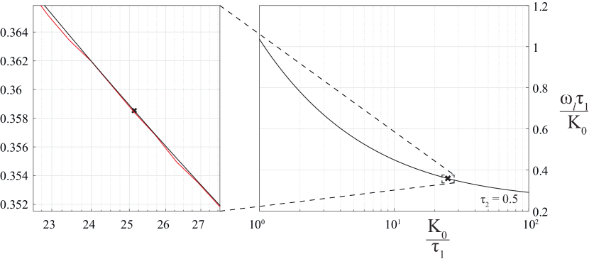
Rigorous derivation of (11 12 13 A 9
Figure 9: Comparison of analytical and numerical results on the lock-in computation.
Appendix A The lock-in computation
In this section equations (11 12 13
{ θ ˙ Δ = y , y ˙ = − a K 0 φ ˙ ( θ Δ ) y − b K 0 φ ( θ Δ ) . cases subscript ˙ 𝜃 Δ 𝑦 otherwise ˙ 𝑦 𝑎 subscript 𝐾 0 ˙ 𝜑 subscript 𝜃 Δ 𝑦 𝑏 subscript 𝐾 0 𝜑 subscript 𝜃 Δ otherwise \begin{cases}\dot{\theta}_{\Delta}=y,\\
\dot{y}=-aK_{0}\dot{\varphi}(\theta_{\Delta})y-bK_{0}\varphi(\theta_{\Delta}).\end{cases} (14)
Also we consider a normalized 2 π 2 𝜋 2\pi
φ ( θ Δ ) = { k θ Δ , if − 1 k ≤ θ Δ ≤ 1 k ; − k π k − 1 θ Δ + π k π k − 1 , if 1 k ≤ θ Δ ≤ 2 π − 1 k 𝜑 subscript 𝜃 Δ cases 𝑘 subscript 𝜃 Δ if − 1 k ≤ θ Δ ≤ 1 k ; 𝑘 𝜋 𝑘 1 subscript 𝜃 Δ 𝜋 𝑘 𝜋 𝑘 1 if 1 k ≤ θ Δ ≤ 2 π − 1 k \varphi(\theta_{\Delta})=\begin{cases}k\theta_{\Delta},&\text{if $-\frac{1}{k}\leq\theta_{\Delta}\leq\frac{1}{k}$;}\\
-\frac{k}{{\pi}k-1}\theta_{\Delta}+\frac{{\pi}k}{{\pi}k-1},&\text{if $\frac{1}{k}\leq\theta_{\Delta}\leq 2\pi-\frac{1}{k}$}\end{cases} (15)
for finite k > 1 π 𝑘 1 𝜋 k>\frac{1}{\pi} θ Δ ∈ [ − 1 k , 2 π − 1 k ) subscript 𝜃 Δ 1 𝑘 2 𝜋 1 𝑘 \theta_{\Delta}\in\left[-\frac{1}{k},2\pi-\frac{1}{k}\right) k = 2 π 𝑘 2 𝜋 k=\frac{2}{\pi} φ ( θ Δ ) 𝜑 subscript 𝜃 Δ \varphi(\theta_{\Delta}) 1
From 2 π 2 𝜋 2\pi 14
θ Δ ∈ ( − 1 k + 2 π j , − 1 k + 2 π ( j + 1 ) ] , j ∈ ℤ . formulae-sequence subscript 𝜃 Δ 1 𝑘 2 𝜋 𝑗 1 𝑘 2 𝜋 𝑗 1 𝑗 ℤ \theta_{\Delta}\in\left(-\frac{1}{k}+2\pi j,-\frac{1}{k}+2\pi(j+1)\right],\hskip 5.69046ptj\in\mathbb{Z}.
Thus, we can consider a single interval ( − 1 k , 2 π − 1 k ] 1 𝑘 2 𝜋 1 𝑘 \left(-\frac{1}{k},2\pi-\frac{1}{k}\right] 14
In the intervals inside ( − 1 k , 2 π − 1 k ] 1 𝑘 2 𝜋 1 𝑘 \left(-\frac{1}{k},2\pi-\frac{1}{k}\right] 14 − 1 k < θ Δ < 1 k 1 𝑘 subscript 𝜃 Δ 1 𝑘 -\frac{1}{k}<\theta_{\Delta}<\frac{1}{k}
{ θ Δ ˙ = y , y ˙ = − a K 0 k y − b K 0 k θ Δ ; cases ˙ subscript 𝜃 Δ 𝑦 otherwise ˙ 𝑦 𝑎 subscript 𝐾 0 𝑘 𝑦 𝑏 subscript 𝐾 0 𝑘 subscript 𝜃 Δ otherwise \displaystyle\begin{cases}\dot{\theta_{\Delta}}=y,\\
\dot{y}=-aK_{0}ky-bK_{0}k\theta_{\Delta};\end{cases} (16)
II. 1 k < θ Δ < 2 π − 1 k 1 𝑘 subscript 𝜃 Δ 2 𝜋 1 𝑘 \frac{1}{k}<\theta_{\Delta}<2\pi-\frac{1}{k}
{ θ Δ ˙ = y , y ˙ = a K 0 k π k − 1 y + b K 0 ( k π k − 1 θ Δ − π k π k − 1 ) . cases ˙ subscript 𝜃 Δ 𝑦 otherwise ˙ 𝑦 𝑎 subscript 𝐾 0 𝑘 𝜋 𝑘 1 𝑦 𝑏 subscript 𝐾 0 𝑘 𝜋 𝑘 1 subscript 𝜃 Δ 𝜋 𝑘 𝜋 𝑘 1 otherwise \displaystyle\begin{cases}\dot{\theta_{\Delta}}=y,\\
\dot{y}=aK_{0}\frac{k}{\pi k-1}y+bK_{0}\left(\frac{k}{\pi k-1}\theta_{\Delta}-\frac{\pi k}{\pi k-1}\right).\end{cases} (17)
In each interval there exists only one equilibrium:
− 1 k < θ Δ < 1 k 1 𝑘 subscript 𝜃 Δ 1 𝑘 -\frac{1}{k}<\theta_{\Delta}<\frac{1}{k}
{ y eq = 0 , − a K 0 k y − b K 0 k θ eq = 0 ; cases subscript 𝑦 eq 0 otherwise 𝑎 subscript 𝐾 0 𝑘 𝑦 𝑏 subscript 𝐾 0 𝑘 subscript 𝜃 eq 0 otherwise \begin{cases}y_{\rm eq}=0,\\
-aK_{0}ky-bK_{0}k\theta_{\rm eq}=0;\end{cases}
{ y eq = 0 , θ eq = 0 ; cases subscript 𝑦 eq 0 otherwise subscript 𝜃 eq 0 otherwise \begin{cases}y_{\rm eq}=0,\\
\theta_{\rm eq}=0;\end{cases}
1 k < θ Δ < 2 π − 1 k 1 𝑘 subscript 𝜃 Δ 2 𝜋 1 𝑘 \frac{1}{k}<\theta_{\Delta}<2\pi-\frac{1}{k}
{ y eq = 0 , a K 0 k π k − 1 y eq + b K 0 k π k − 1 ( θ eq − π ) = 0 . cases subscript 𝑦 eq 0 otherwise 𝑎 subscript 𝐾 0 𝑘 𝜋 𝑘 1 subscript 𝑦 eq 𝑏 subscript 𝐾 0 𝑘 𝜋 𝑘 1 subscript 𝜃 eq 𝜋 0 otherwise \begin{cases}y_{\rm eq}=0,\\
\frac{aK_{0}k}{\pi k-1}y_{\rm eq}+\frac{bK_{0}k}{\pi k-1}\left(\theta_{\rm eq}-\pi\right)=0.\end{cases}
{ y eq = 0 , θ eq = π . cases subscript 𝑦 eq 0 otherwise subscript 𝜃 eq 𝜋 otherwise \begin{cases}y_{\rm eq}=0,\\
\theta_{\rm eq}=\pi.\end{cases}
To define a type of the equilibria points, we compute the corresponding characteristic polynomial and eigenvalues. For the first equilibrium ( θ eq , y eq ) = ( 0 , 0 ) subscript 𝜃 eq subscript 𝑦 eq 0 0 (\theta_{\rm eq},y_{\rm eq})=\left(0,0\right)
χ ( λ ) = | − λ 1 − b K 0 k − a K 0 k − λ | = λ 2 + a K 0 k λ + b K 0 k . 𝜒 𝜆 𝜆 1 𝑏 subscript 𝐾 0 𝑘 𝑎 subscript 𝐾 0 𝑘 𝜆 superscript 𝜆 2 𝑎 subscript 𝐾 0 𝑘 𝜆 𝑏 subscript 𝐾 0 𝑘 \chi(\lambda)=\left|\begin{array}[]{cc}-\lambda&1\\
-bK_{0}k&-aK_{0}k-\lambda\end{array}\right|=\lambda^{2}+aK_{0}k\lambda+{b}K_{0}k.
The eigenvalues of the equilibrium ( θ eq , y eq ) = ( 0 , 0 ) subscript 𝜃 eq subscript 𝑦 eq 0 0 (\theta_{\rm eq},y_{\rm eq})=\left(0,0\right) ( a K 0 ) 2 − 4 b K 0 k superscript 𝑎 subscript 𝐾 0 2 4 𝑏 subscript 𝐾 0 𝑘 (aK_{0})^{2}-\frac{4bK_{0}}{k} A. ( a K 0 ) 2 − 4 b K 0 k > 0 superscript 𝑎 subscript 𝐾 0 2 4 𝑏 subscript 𝐾 0 𝑘 0 (aK_{0})^{2}-\frac{4bK_{0}}{k}>0
λ 1 , 2 s = − a K 0 k ± ( a K 0 k ) 2 − 4 b K 0 k 2 , subscript superscript 𝜆 𝑠 1 2
plus-or-minus 𝑎 subscript 𝐾 0 𝑘 superscript 𝑎 subscript 𝐾 0 𝑘 2 4 𝑏 subscript 𝐾 0 𝑘 2 \lambda^{s}_{1,2}=\displaystyle\frac{-aK_{0}k\pm\sqrt{(aK_{0}k)^{2}-4{b}K_{0}k}}{2},
the equilibrium ( 0 , 0 ) 0 0 \left(0,0\right) B. ( a K 0 ) 2 − 4 b K 0 k = 0 superscript 𝑎 subscript 𝐾 0 2 4 𝑏 subscript 𝐾 0 𝑘 0 (aK_{0})^{2}-\frac{4bK_{0}}{k}=0
λ 1 s = λ 2 s = − a K 0 k 2 , subscript superscript 𝜆 𝑠 1 subscript superscript 𝜆 𝑠 2 𝑎 subscript 𝐾 0 𝑘 2 \lambda^{s}_{1}=\lambda^{s}_{2}=\displaystyle\frac{-aK_{0}k}{2},
the equilibrium ( 0 , 0 ) 0 0 \left(0,0\right) C. ( a K 0 ) 2 − 4 b K 0 k < 0 superscript 𝑎 subscript 𝐾 0 2 4 𝑏 subscript 𝐾 0 𝑘 0 (aK_{0})^{2}-\frac{4bK_{0}}{k}<0
λ 1 , 2 s = − a K 0 k ± i 4 b K 0 k − ( a K 0 k ) 2 2 , subscript superscript 𝜆 𝑠 1 2
plus-or-minus 𝑎 subscript 𝐾 0 𝑘 𝑖 4 𝑏 subscript 𝐾 0 𝑘 superscript 𝑎 subscript 𝐾 0 𝑘 2 2 \lambda^{s}_{1,2}=\displaystyle\frac{-aK_{0}k\pm i\sqrt{4{b}K_{0}k-(aK_{0}k)^{2}}}{2},
the equilibrium ( 0 , 0 ) 0 0 \left(0,0\right) ( θ eq s , y eq ) = ( 0 , 0 ) subscript superscript 𝜃 𝑠 eq subscript 𝑦 eq 0 0 (\theta^{s}_{\rm eq},y_{\rm eq})=(0,0)
For the second equilibrium ( θ eq , y eq ) = ( π , 0 ) subscript 𝜃 eq subscript 𝑦 eq 𝜋 0 (\theta_{\rm eq},y_{\rm eq})=\left(\pi,0\right)
χ ( λ ) = | − λ 1 b K 0 k π k − 1 a K 0 k π k − 1 − λ | = λ 2 − a K 0 k π k − 1 λ − b K 0 k π k − 1 ; 𝜒 𝜆 𝜆 1 𝑏 subscript 𝐾 0 𝑘 𝜋 𝑘 1 𝑎 subscript 𝐾 0 𝑘 𝜋 𝑘 1 𝜆 superscript 𝜆 2 𝑎 subscript 𝐾 0 𝑘 𝜋 𝑘 1 𝜆 𝑏 subscript 𝐾 0 𝑘 𝜋 𝑘 1 \displaystyle\chi(\lambda)=\left|\begin{array}[]{cc}-\lambda&1\\
\frac{bK_{0}k}{\pi k-1}&\frac{aK_{0}k}{\pi k-1}-\lambda\end{array}\right|=\lambda^{2}-\frac{aK_{0}k}{\pi k-1}\lambda-\frac{bK_{0}k}{\pi k-1};
λ 1 , 2 u = a K 0 k π k − 1 ± ( a K 0 k π k − 1 ) 2 + 4 b K 0 k π k − 1 2 , subscript superscript 𝜆 𝑢 1 2
plus-or-minus 𝑎 subscript 𝐾 0 𝑘 𝜋 𝑘 1 superscript 𝑎 subscript 𝐾 0 𝑘 𝜋 𝑘 1 2 4 𝑏 subscript 𝐾 0 𝑘 𝜋 𝑘 1 2 \displaystyle\lambda^{u}_{1,2}=\displaystyle\frac{\frac{aK_{0}k}{{\pi}k-1}\pm\sqrt{\left(\frac{aK_{0}k}{{\pi}k-1}\right)^{2}+\frac{4{b}K_{0}k}{{\pi}k-1}}}{2},
which means that ( π , 0 ) 𝜋 0 \left(\pi,0\right) ( θ eq u , y eq ) = ( π , 0 ) subscript superscript 𝜃 𝑢 eq subscript 𝑦 eq 𝜋 0 (\theta^{u}_{\rm eq},y_{\rm eq})=(\pi,0)
The calculation of S ′ ( θ eq s ) superscript 𝑆 ′ subscript superscript 𝜃 𝑠 eq S^{\prime}(\theta^{s}_{\rm eq}) 10 X 1 u subscript superscript 𝑋 𝑢 1 X^{u}_{1} X 2 u subscript superscript 𝑋 𝑢 2 X^{u}_{2} ( θ eq u , y eq ) subscript superscript 𝜃 𝑢 eq subscript 𝑦 eq \left(\theta^{u}_{\rm eq},y_{\rm eq}\right) θ Δ ∈ ( 1 k , 2 π − 1 k ) subscript 𝜃 Δ 1 𝑘 2 𝜋 1 𝑘 \theta_{\Delta}\in\left(\frac{1}{k},2\pi-\frac{1}{k}\right) S ′ ( 1 k ) superscript 𝑆 ′ 1 𝑘 S^{\prime}(\frac{1}{k}) 14 X 1 s subscript superscript 𝑋 𝑠 1 X^{s}_{1} X 2 s subscript superscript 𝑋 𝑠 2 X^{s}_{2} ( θ eq s , y eq ) subscript superscript 𝜃 𝑠 eq subscript 𝑦 eq \left(\theta^{s}_{\rm eq},y_{\rm eq}\right) θ Δ ∈ ( − 1 k , 1 k ) subscript 𝜃 Δ 1 𝑘 1 𝑘 \theta_{\Delta}\in\left(-\frac{1}{k},\frac{1}{k}\right) 14 θ Δ ∈ ( − 1 k , 1 k ) subscript 𝜃 Δ 1 𝑘 1 𝑘 \theta_{\Delta}\in\left(-\frac{1}{k},\frac{1}{k}\right) S ′ ( 1 k ) superscript 𝑆 ′ 1 𝑘 S^{\prime}(\frac{1}{k}) S ′ ( θ eq s ) superscript 𝑆 ′ subscript superscript 𝜃 𝑠 eq S^{\prime}(\theta^{s}_{\rm eq})
Let us find the eigenvectors X 1 u subscript superscript 𝑋 𝑢 1 X^{u}_{1} X 2 u subscript superscript 𝑋 𝑢 2 X^{u}_{2} ( θ eq u , y eq ) subscript superscript 𝜃 𝑢 eq subscript 𝑦 eq \left(\theta^{u}_{\rm eq},y_{\rm eq}\right) X 1 u subscript superscript 𝑋 𝑢 1 X^{u}_{1}
( − λ 1 u 1 b K 0 k π k − 1 a K 0 k π k − 1 − λ 1 u ) X 1 u = 𝕆 , subscript superscript 𝜆 𝑢 1 1 𝑏 subscript 𝐾 0 𝑘 𝜋 𝑘 1 𝑎 subscript 𝐾 0 𝑘 𝜋 𝑘 1 subscript superscript 𝜆 𝑢 1 subscript superscript 𝑋 𝑢 1 𝕆 \displaystyle\left(\begin{array}[]{cc}-\lambda^{u}_{1}&1\\
\frac{bK_{0}k}{\pi k-1}&\frac{aK_{0}k}{\pi k-1}-\lambda^{u}_{1}\end{array}\right)X^{u}_{1}=\mathbb{O},
( − a K 0 k π k − 1 + ( a K 0 k π k − 1 ) 2 + 4 b K 0 k π k − 1 2 1 b K 0 k π k − 1 a K 0 k π k − 1 − a K 0 k π k − 1 + ( a K 0 k π k − 1 ) 2 + 4 b K 0 k π k − 1 2 ) X 1 u = 𝕆 , 𝑎 subscript 𝐾 0 𝑘 𝜋 𝑘 1 superscript 𝑎 subscript 𝐾 0 𝑘 𝜋 𝑘 1 2 4 𝑏 subscript 𝐾 0 𝑘 𝜋 𝑘 1 2 1 𝑏 subscript 𝐾 0 𝑘 𝜋 𝑘 1 𝑎 subscript 𝐾 0 𝑘 𝜋 𝑘 1 𝑎 subscript 𝐾 0 𝑘 𝜋 𝑘 1 superscript 𝑎 subscript 𝐾 0 𝑘 𝜋 𝑘 1 2 4 𝑏 subscript 𝐾 0 𝑘 𝜋 𝑘 1 2 subscript superscript 𝑋 𝑢 1 𝕆 \displaystyle\left(\begin{array}[]{cc}-\displaystyle\frac{\frac{aK_{0}k}{{\pi}k-1}+\sqrt{\left(\frac{aK_{0}k}{{\pi}k-1}\right)^{2}+\frac{4{b}K_{0}k}{{\pi}k-1}}}{2}&1\\
\frac{bK_{0}k}{\pi k-1}&\frac{aK_{0}k}{\pi k-1}-\displaystyle\frac{\frac{aK_{0}k}{{\pi}k-1}+\sqrt{\left(\frac{aK_{0}k}{{\pi}k-1}\right)^{2}+\frac{4{b}K_{0}k}{{\pi}k-1}}}{2}\end{array}\right)X^{u}_{1}=\mathbb{O},
( − a K 0 k π k − 1 + ( a K 0 k π k − 1 ) 2 + 4 b K 0 k π k − 1 2 1 b K 0 k π k − 1 − a K 0 k π k − 1 − ( a K 0 k π k − 1 ) 2 + 4 b K 0 k π k − 1 2 ) X 1 u = 𝕆 . 𝑎 subscript 𝐾 0 𝑘 𝜋 𝑘 1 superscript 𝑎 subscript 𝐾 0 𝑘 𝜋 𝑘 1 2 4 𝑏 subscript 𝐾 0 𝑘 𝜋 𝑘 1 2 1 𝑏 subscript 𝐾 0 𝑘 𝜋 𝑘 1 𝑎 subscript 𝐾 0 𝑘 𝜋 𝑘 1 superscript 𝑎 subscript 𝐾 0 𝑘 𝜋 𝑘 1 2 4 𝑏 subscript 𝐾 0 𝑘 𝜋 𝑘 1 2 subscript superscript 𝑋 𝑢 1 𝕆 \displaystyle\left(\begin{array}[]{cc}-\displaystyle\frac{\frac{aK_{0}k}{{\pi}k-1}+\sqrt{\left(\frac{aK_{0}k}{{\pi}k-1}\right)^{2}+\frac{4{b}K_{0}k}{{\pi}k-1}}}{2}&1\\
\frac{bK_{0}k}{\pi k-1}&-\displaystyle\frac{\frac{aK_{0}k}{{\pi}k-1}-\sqrt{\left(\frac{aK_{0}k}{{\pi}k-1}\right)^{2}+\frac{4{b}K_{0}k}{{\pi}k-1}}}{2}\end{array}\right)X^{u}_{1}=\mathbb{O}. (20)
Multiply the second row of (20 a K 0 k π k − 1 + ( a K 0 k π k − 1 ) 2 + 4 b K 0 k π k − 1 2 𝑎 subscript 𝐾 0 𝑘 𝜋 𝑘 1 superscript 𝑎 subscript 𝐾 0 𝑘 𝜋 𝑘 1 2 4 𝑏 subscript 𝐾 0 𝑘 𝜋 𝑘 1 2 \displaystyle\frac{\frac{aK_{0}k}{{\pi}k-1}+\sqrt{\left(\frac{aK_{0}k}{{\pi}k-1}\right)^{2}+\frac{4{b}K_{0}k}{{\pi}k-1}}}{2} b K 0 k π k − 1 𝑏 subscript 𝐾 0 𝑘 𝜋 𝑘 1 \displaystyle\frac{bK_{0}k}{\pi k-1}
( − a K 0 k π k − 1 + ( a K 0 k π k − 1 ) 2 + 4 b K 0 k π k − 1 2 1 a K 0 k π k − 1 + ( a K 0 k π k − 1 ) 2 + 4 b K 0 k π k − 1 2 − ( ( a K 0 k π k − 1 ) 2 − ( a K 0 k π k − 1 ) 2 + 4 b K 0 k π k − 1 ) ( π k − 1 ) 4 b K 0 k ) X 1 u = 𝕆 , 𝑎 subscript 𝐾 0 𝑘 𝜋 𝑘 1 superscript 𝑎 subscript 𝐾 0 𝑘 𝜋 𝑘 1 2 4 𝑏 subscript 𝐾 0 𝑘 𝜋 𝑘 1 2 1 𝑎 subscript 𝐾 0 𝑘 𝜋 𝑘 1 superscript 𝑎 subscript 𝐾 0 𝑘 𝜋 𝑘 1 2 4 𝑏 subscript 𝐾 0 𝑘 𝜋 𝑘 1 2 superscript 𝑎 subscript 𝐾 0 𝑘 𝜋 𝑘 1 2 superscript 𝑎 subscript 𝐾 0 𝑘 𝜋 𝑘 1 2 4 𝑏 subscript 𝐾 0 𝑘 𝜋 𝑘 1 𝜋 𝑘 1 4 𝑏 subscript 𝐾 0 𝑘 subscript superscript 𝑋 𝑢 1 𝕆 \displaystyle\left(\begin{array}[]{cc}-\displaystyle\frac{\frac{aK_{0}k}{{\pi}k-1}+\sqrt{\left(\frac{aK_{0}k}{{\pi}k-1}\right)^{2}+\frac{4{b}K_{0}k}{{\pi}k-1}}}{2}&1\\
\displaystyle\frac{\frac{aK_{0}k}{{\pi}k-1}+\sqrt{\left(\frac{aK_{0}k}{{\pi}k-1}\right)^{2}+\frac{4{b}K_{0}k}{{\pi}k-1}}}{2}&-\displaystyle\frac{\left(\left(\frac{aK_{0}k}{{\pi}k-1}\right)^{2}-(\frac{aK_{0}k}{{\pi}k-1})^{2}+\frac{4{b}K_{0}k}{{\pi}k-1}\right)\left({\pi}k-1\right)}{4bK_{0}k}\end{array}\right)X^{u}_{1}=\mathbb{O},
( − a K 0 k π k − 1 + ( a K 0 k π k − 1 ) 2 + 4 b K 0 k π k − 1 2 1 a K 0 k π k − 1 + ( a K 0 k π k − 1 ) 2 + 4 b K 0 k π k − 1 2 − 1 ) X 1 u = 𝕆 . 𝑎 subscript 𝐾 0 𝑘 𝜋 𝑘 1 superscript 𝑎 subscript 𝐾 0 𝑘 𝜋 𝑘 1 2 4 𝑏 subscript 𝐾 0 𝑘 𝜋 𝑘 1 2 1 𝑎 subscript 𝐾 0 𝑘 𝜋 𝑘 1 superscript 𝑎 subscript 𝐾 0 𝑘 𝜋 𝑘 1 2 4 𝑏 subscript 𝐾 0 𝑘 𝜋 𝑘 1 2 1 subscript superscript 𝑋 𝑢 1 𝕆 \displaystyle\left(\begin{array}[]{cc}-\displaystyle\frac{\frac{aK_{0}k}{{\pi}k-1}+\sqrt{\left(\frac{aK_{0}k}{{\pi}k-1}\right)^{2}+\frac{4{b}K_{0}k}{{\pi}k-1}}}{2}&1\\
\displaystyle\frac{\frac{aK_{0}k}{{\pi}k-1}+\sqrt{\left(\frac{aK_{0}k}{{\pi}k-1}\right)^{2}+\frac{4{b}K_{0}k}{{\pi}k-1}}}{2}&-1\end{array}\right)X^{u}_{1}=\mathbb{O}.
Hence,
X 1 u = ( c c ( a K 0 k ) 2 + 4 b K 0 k ( π k − 1 ) + a K 0 k 2 ( π k − 1 ) ) . subscript superscript 𝑋 𝑢 1 𝑐 𝑐 superscript 𝑎 subscript 𝐾 0 𝑘 2 4 𝑏 subscript 𝐾 0 𝑘 𝜋 𝑘 1 𝑎 subscript 𝐾 0 𝑘 2 𝜋 𝑘 1 X^{u}_{1}=\left(\begin{array}[]{c}c\\
\displaystyle c\frac{\sqrt{(aK_{0}k)^{2}+4{b}K_{0}k({\pi}k-1)}+aK_{0}k}{2({\pi}k-1)}\end{array}\right).
Let us choose c = ( a K 0 k ) 2 + 4 b K 0 k ( π k − 1 ) − a K 0 k 2 b K 0 k 𝑐 superscript 𝑎 subscript 𝐾 0 𝑘 2 4 𝑏 subscript 𝐾 0 𝑘 𝜋 𝑘 1 𝑎 subscript 𝐾 0 𝑘 2 𝑏 subscript 𝐾 0 𝑘 c=\displaystyle\frac{\sqrt{(aK_{0}k)^{2}+4{b}K_{0}k({\pi}k-1)}-aK_{0}k}{2bK_{0}k}
X 1 u = ( ( a K 0 k ) 2 + 4 b K 0 k ( π k − 1 ) − a K 0 k 2 b K 0 k ( a K 0 k ) 2 + 4 b K 0 k ( π k − 1 ) − ( a K 0 k ) 2 4 b K 0 k ( π k − 1 ) ) , subscript superscript 𝑋 𝑢 1 superscript 𝑎 subscript 𝐾 0 𝑘 2 4 𝑏 subscript 𝐾 0 𝑘 𝜋 𝑘 1 𝑎 subscript 𝐾 0 𝑘 2 𝑏 subscript 𝐾 0 𝑘 superscript 𝑎 subscript 𝐾 0 𝑘 2 4 𝑏 subscript 𝐾 0 𝑘 𝜋 𝑘 1 superscript 𝑎 subscript 𝐾 0 𝑘 2 4 𝑏 subscript 𝐾 0 𝑘 𝜋 𝑘 1 \displaystyle X^{u}_{1}=\left(\begin{array}[]{c}\displaystyle\frac{\sqrt{(aK_{0}k)^{2}+4{b}K_{0}k({\pi}k-1)}-aK_{0}k}{2bK_{0}k}\\
\displaystyle\frac{(aK_{0}k)^{2}+4{b}K_{0}k({\pi}k-1)-(aK_{0}k)^{2}}{4bK_{0}k({\pi}k-1)}\end{array}\right),
X 1 u = ( ( a K 0 k ) 2 + 4 b K 0 k ( π k − 1 ) − a K 0 k 2 b K 0 k 1 ) . subscript superscript 𝑋 𝑢 1 superscript 𝑎 subscript 𝐾 0 𝑘 2 4 𝑏 subscript 𝐾 0 𝑘 𝜋 𝑘 1 𝑎 subscript 𝐾 0 𝑘 2 𝑏 subscript 𝐾 0 𝑘 1 \displaystyle X^{u}_{1}=\left(\begin{array}[]{c}\displaystyle\frac{\sqrt{(aK_{0}k)^{2}+4{b}K_{0}k({\pi}k-1)}-aK_{0}k}{2bK_{0}k}\\
1\end{array}\right).
Next, find the second eigenvector X 2 u subscript superscript 𝑋 𝑢 2 X^{u}_{2}
( − λ 2 u 1 b K 0 k π k − 1 a K 0 k π k − 1 − λ 2 u ) X 2 u = 𝕆 , subscript superscript 𝜆 𝑢 2 1 𝑏 subscript 𝐾 0 𝑘 𝜋 𝑘 1 𝑎 subscript 𝐾 0 𝑘 𝜋 𝑘 1 subscript superscript 𝜆 𝑢 2 subscript superscript 𝑋 𝑢 2 𝕆 \displaystyle\left(\begin{array}[]{cc}-\lambda^{u}_{2}&1\\
\frac{bK_{0}k}{\pi k-1}&\frac{aK_{0}k}{\pi k-1}-\lambda^{u}_{2}\end{array}\right)X^{u}_{2}=\mathbb{O},
( ( a K 0 k π k − 1 ) 2 + 4 b K 0 k π k − 1 − a K 0 k π k − 1 2 1 b K 0 k π k − 1 a K 0 k π k − 1 + ( a K 0 k π k − 1 ) 2 + 4 b K 0 k π k − 1 − a K 0 k π k − 1 2 ) X 2 u = 𝕆 , superscript 𝑎 subscript 𝐾 0 𝑘 𝜋 𝑘 1 2 4 𝑏 subscript 𝐾 0 𝑘 𝜋 𝑘 1 𝑎 subscript 𝐾 0 𝑘 𝜋 𝑘 1 2 1 𝑏 subscript 𝐾 0 𝑘 𝜋 𝑘 1 𝑎 subscript 𝐾 0 𝑘 𝜋 𝑘 1 superscript 𝑎 subscript 𝐾 0 𝑘 𝜋 𝑘 1 2 4 𝑏 subscript 𝐾 0 𝑘 𝜋 𝑘 1 𝑎 subscript 𝐾 0 𝑘 𝜋 𝑘 1 2 subscript superscript 𝑋 𝑢 2 𝕆 \displaystyle\left(\begin{array}[]{cc}\displaystyle\frac{\sqrt{\left(\frac{aK_{0}k}{{\pi}k-1}\right)^{2}+\frac{4{b}K_{0}k}{{\pi}k-1}}-\frac{aK_{0}k}{{\pi}k-1}}{2}&1\\
\frac{bK_{0}k}{\pi k-1}&\frac{aK_{0}k}{\pi k-1}+\displaystyle\frac{\sqrt{\left(\frac{aK_{0}k}{{\pi}k-1}\right)^{2}+\frac{4{b}K_{0}k}{{\pi}k-1}}-\frac{aK_{0}k}{{\pi}k-1}}{2}\end{array}\right)X^{u}_{2}=\mathbb{O},
( ( a K 0 k π k − 1 ) 2 + 4 b K 0 k π k − 1 − a K 0 k π k − 1 2 1 b K 0 k π k − 1 ( a K 0 k π k − 1 ) 2 + 4 b K 0 k π k − 1 + a K 0 k π k − 1 2 ) X 2 u = 𝕆 . superscript 𝑎 subscript 𝐾 0 𝑘 𝜋 𝑘 1 2 4 𝑏 subscript 𝐾 0 𝑘 𝜋 𝑘 1 𝑎 subscript 𝐾 0 𝑘 𝜋 𝑘 1 2 1 𝑏 subscript 𝐾 0 𝑘 𝜋 𝑘 1 superscript 𝑎 subscript 𝐾 0 𝑘 𝜋 𝑘 1 2 4 𝑏 subscript 𝐾 0 𝑘 𝜋 𝑘 1 𝑎 subscript 𝐾 0 𝑘 𝜋 𝑘 1 2 subscript superscript 𝑋 𝑢 2 𝕆 \displaystyle\left(\begin{array}[]{cc}\displaystyle\frac{\sqrt{\left(\frac{aK_{0}k}{{\pi}k-1}\right)^{2}+\frac{4{b}K_{0}k}{{\pi}k-1}}-\frac{aK_{0}k}{{\pi}k-1}}{2}&1\\
\frac{bK_{0}k}{\pi k-1}&\displaystyle\frac{\sqrt{\left(\frac{aK_{0}k}{{\pi}k-1}\right)^{2}+\frac{4{b}K_{0}k}{{\pi}k-1}}+\frac{aK_{0}k}{{\pi}k-1}}{2}\end{array}\right)X^{u}_{2}=\mathbb{O}. (23)
Multiply the second row of (23 ( a K 0 k π k − 1 ) 2 + 4 b K 0 k π k − 1 − a K 0 k π k − 1 2 superscript 𝑎 subscript 𝐾 0 𝑘 𝜋 𝑘 1 2 4 𝑏 subscript 𝐾 0 𝑘 𝜋 𝑘 1 𝑎 subscript 𝐾 0 𝑘 𝜋 𝑘 1 2 \displaystyle\frac{\sqrt{\left(\frac{aK_{0}k}{{\pi}k-1}\right)^{2}+\frac{4{b}K_{0}k}{{\pi}k-1}}-\frac{aK_{0}k}{{\pi}k-1}}{2} b K 0 k π k − 1 𝑏 subscript 𝐾 0 𝑘 𝜋 𝑘 1 \displaystyle\frac{bK_{0}k}{\pi k-1}
( ( a K 0 k π k − 1 ) 2 + 4 b K 0 k π k − 1 − a K 0 k π k − 1 2 1 ( a K 0 k π k − 1 ) 2 + 4 b K 0 k π k − 1 − a K 0 k π k − 1 2 ( ( a K 0 k π k − 1 ) 2 + 4 b K 0 k π k − 1 − ( a K 0 k π k − 1 ) 2 ) ( π k − 1 ) 4 b K 0 k ) X 2 u = 𝕆 , superscript 𝑎 subscript 𝐾 0 𝑘 𝜋 𝑘 1 2 4 𝑏 subscript 𝐾 0 𝑘 𝜋 𝑘 1 𝑎 subscript 𝐾 0 𝑘 𝜋 𝑘 1 2 1 superscript 𝑎 subscript 𝐾 0 𝑘 𝜋 𝑘 1 2 4 𝑏 subscript 𝐾 0 𝑘 𝜋 𝑘 1 𝑎 subscript 𝐾 0 𝑘 𝜋 𝑘 1 2 superscript 𝑎 subscript 𝐾 0 𝑘 𝜋 𝑘 1 2 4 𝑏 subscript 𝐾 0 𝑘 𝜋 𝑘 1 superscript 𝑎 subscript 𝐾 0 𝑘 𝜋 𝑘 1 2 𝜋 𝑘 1 4 𝑏 subscript 𝐾 0 𝑘 subscript superscript 𝑋 𝑢 2 𝕆 \displaystyle\left(\begin{array}[]{cc}\displaystyle\frac{\sqrt{\left(\frac{aK_{0}k}{{\pi}k-1}\right)^{2}+\frac{4{b}K_{0}k}{{\pi}k-1}}-\frac{aK_{0}k}{{\pi}k-1}}{2}&1\\
\displaystyle\frac{\sqrt{\left(\frac{aK_{0}k}{{\pi}k-1}\right)^{2}+\frac{4{b}K_{0}k}{{\pi}k-1}}-\frac{aK_{0}k}{{\pi}k-1}}{2}&\displaystyle\frac{\left(\left(\frac{aK_{0}k}{{\pi}k-1}\right)^{2}+\frac{4{b}K_{0}k}{{\pi}k-1}-\left(\frac{aK_{0}k}{{\pi}k-1}\right)^{2}\right)\left({\pi}k-1\right)}{4bK_{0}k}\end{array}\right)X^{u}_{2}=\mathbb{O},
( ( a K 0 k π k − 1 ) 2 + 4 b K 0 k π k − 1 − a K 0 k π k − 1 2 1 ( a K 0 k π k − 1 ) 2 + 4 b K 0 k π k − 1 − a K 0 k π k − 1 2 1 ) X 2 u = 𝕆 . superscript 𝑎 subscript 𝐾 0 𝑘 𝜋 𝑘 1 2 4 𝑏 subscript 𝐾 0 𝑘 𝜋 𝑘 1 𝑎 subscript 𝐾 0 𝑘 𝜋 𝑘 1 2 1 superscript 𝑎 subscript 𝐾 0 𝑘 𝜋 𝑘 1 2 4 𝑏 subscript 𝐾 0 𝑘 𝜋 𝑘 1 𝑎 subscript 𝐾 0 𝑘 𝜋 𝑘 1 2 1 subscript superscript 𝑋 𝑢 2 𝕆 \displaystyle\left(\begin{array}[]{cc}\displaystyle\frac{\sqrt{\left(\frac{aK_{0}k}{{\pi}k-1}\right)^{2}+\frac{4{b}K_{0}k}{{\pi}k-1}}-\frac{aK_{0}k}{{\pi}k-1}}{2}&1\\
\displaystyle\frac{\sqrt{\left(\frac{aK_{0}k}{{\pi}k-1}\right)^{2}+\frac{4{b}K_{0}k}{{\pi}k-1}}-\frac{aK_{0}k}{{\pi}k-1}}{2}&1\end{array}\right)X^{u}_{2}=\mathbb{O}.
Hence,
X 2 u = ( − c c ( a K 0 k π k − 1 ) 2 + 4 b K 0 k π k − 1 − a K 0 k π k − 1 2 ) . subscript superscript 𝑋 𝑢 2 𝑐 𝑐 superscript 𝑎 subscript 𝐾 0 𝑘 𝜋 𝑘 1 2 4 𝑏 subscript 𝐾 0 𝑘 𝜋 𝑘 1 𝑎 subscript 𝐾 0 𝑘 𝜋 𝑘 1 2 X^{u}_{2}=\left(\begin{array}[]{c}-c\\
\displaystyle c\frac{\sqrt{\left(\frac{aK_{0}k}{{\pi}k-1}\right)^{2}+\frac{4{b}K_{0}k}{{\pi}k-1}}-\frac{aK_{0}k}{{\pi}k-1}}{2}\end{array}\right).
Choose c = ( a K 0 k ) 2 + 4 b K 0 k ( π k − 1 ) + a K 0 k 2 b K 0 k 𝑐 superscript 𝑎 subscript 𝐾 0 𝑘 2 4 𝑏 subscript 𝐾 0 𝑘 𝜋 𝑘 1 𝑎 subscript 𝐾 0 𝑘 2 𝑏 subscript 𝐾 0 𝑘 c=\displaystyle\frac{\sqrt{(aK_{0}k)^{2}+4{b}K_{0}k({\pi}k-1)}+aK_{0}k}{2bK_{0}k}
X 2 u = ( − ( a K 0 k ) 2 + 4 b K 0 k ( π k − 1 ) + a K 0 k 2 b K 0 k ( a K 0 k ) 2 + 4 b K 0 k ( π k − 1 ) − ( a K 0 k ) 2 4 b K 0 k ( π k − 1 ) ) , subscript superscript 𝑋 𝑢 2 superscript 𝑎 subscript 𝐾 0 𝑘 2 4 𝑏 subscript 𝐾 0 𝑘 𝜋 𝑘 1 𝑎 subscript 𝐾 0 𝑘 2 𝑏 subscript 𝐾 0 𝑘 superscript 𝑎 subscript 𝐾 0 𝑘 2 4 𝑏 subscript 𝐾 0 𝑘 𝜋 𝑘 1 superscript 𝑎 subscript 𝐾 0 𝑘 2 4 𝑏 subscript 𝐾 0 𝑘 𝜋 𝑘 1 \displaystyle X^{u}_{2}=\left(\begin{array}[]{c}\displaystyle-\frac{\sqrt{(aK_{0}k)^{2}+4{b}K_{0}k({\pi}k-1)}+aK_{0}k}{2bK_{0}k}\\
\displaystyle\frac{(aK_{0}k)^{2}+4{b}K_{0}k({\pi}k-1)-(aK_{0}k)^{2}}{4bK_{0}k({\pi}k-1)}\end{array}\right),
X 2 u = ( − ( a K 0 k ) 2 + 4 b K 0 k ( π k − 1 ) + a K 0 k 2 b K 0 k 1 ) . subscript superscript 𝑋 𝑢 2 superscript 𝑎 subscript 𝐾 0 𝑘 2 4 𝑏 subscript 𝐾 0 𝑘 𝜋 𝑘 1 𝑎 subscript 𝐾 0 𝑘 2 𝑏 subscript 𝐾 0 𝑘 1 \displaystyle X^{u}_{2}=\left(\begin{array}[]{c}\displaystyle-\frac{\sqrt{(aK_{0}k)^{2}+4{b}K_{0}k({\pi}k-1)}+aK_{0}k}{2bK_{0}k}\\
1\end{array}\right).
We can show that the direction of separatrix S ′ ( θ Δ ) superscript 𝑆 ′ subscript 𝜃 Δ S^{\prime}(\theta_{\Delta}) X 2 u subscript superscript 𝑋 𝑢 2 X^{u}_{2} λ 2 u subscript superscript 𝜆 𝑢 2 \lambda^{u}_{2} S ′ ( 1 k ) superscript 𝑆 ′ 1 𝑘 S^{\prime}(\frac{1}{k})
( x 1 , y 1 ) = ( π , 0 ) , subscript 𝑥 1 subscript 𝑦 1 𝜋 0 \displaystyle\left(x_{1},y_{1}\right)=\left(\pi,0\right),
( x 2 , y 2 ) = ( π − ( a K 0 k ) 2 + 4 b K 0 k ( π k − 1 ) + a K 0 k 2 b K 0 k , 1 ) . subscript 𝑥 2 subscript 𝑦 2 𝜋 superscript 𝑎 subscript 𝐾 0 𝑘 2 4 𝑏 subscript 𝐾 0 𝑘 𝜋 𝑘 1 𝑎 subscript 𝐾 0 𝑘 2 𝑏 subscript 𝐾 0 𝑘 1 \displaystyle\left(x_{2},y_{2}\right)=\left(\pi-\displaystyle\frac{\sqrt{(aK_{0}k)^{2}+4{b}K_{0}k({\pi}k-1)}+aK_{0}k}{2bK_{0}k},1\right).
The equation takes the form
y − 0 1 − 0 = x − π ( π − ( a K 0 k ) 2 + 4 b K 0 k ( π k − 1 ) + a K 0 k 2 b K 0 k ) − π , 𝑦 0 1 0 𝑥 𝜋 𝜋 superscript 𝑎 subscript 𝐾 0 𝑘 2 4 𝑏 subscript 𝐾 0 𝑘 𝜋 𝑘 1 𝑎 subscript 𝐾 0 𝑘 2 𝑏 subscript 𝐾 0 𝑘 𝜋 \displaystyle\frac{y-0}{1-0}=\frac{x-\pi}{\left(\pi-\displaystyle\frac{\sqrt{(aK_{0}k)^{2}+4{b}K_{0}k({\pi}k-1)}+aK_{0}k}{2bK_{0}k}\right)-\pi},
y = 2 b K 0 k ( a K 0 k ) 2 + 4 b K 0 k ( π k − 1 ) + a K 0 k ( π − x ) , 𝑦 2 𝑏 subscript 𝐾 0 𝑘 superscript 𝑎 subscript 𝐾 0 𝑘 2 4 𝑏 subscript 𝐾 0 𝑘 𝜋 𝑘 1 𝑎 subscript 𝐾 0 𝑘 𝜋 𝑥 \displaystyle y=\frac{2bK_{0}k}{\sqrt{(aK_{0}k)^{2}+4{b}K_{0}k({\pi}k-1)}+aK_{0}k}\left(\pi-x\right),
y = 2 b K 0 k ( ( a K 0 k ) 2 + 4 b K 0 k ( π k − 1 ) − a K 0 k ) ( a K 0 k ) 2 + 4 b K 0 k ( π k − 1 ) − ( a K 0 k ) 2 ( π − x ) , 𝑦 2 𝑏 subscript 𝐾 0 𝑘 superscript 𝑎 subscript 𝐾 0 𝑘 2 4 𝑏 subscript 𝐾 0 𝑘 𝜋 𝑘 1 𝑎 subscript 𝐾 0 𝑘 superscript 𝑎 subscript 𝐾 0 𝑘 2 4 𝑏 subscript 𝐾 0 𝑘 𝜋 𝑘 1 superscript 𝑎 subscript 𝐾 0 𝑘 2 𝜋 𝑥 \displaystyle y=\frac{2bK_{0}k\left(\sqrt{(aK_{0}k)^{2}+4{b}K_{0}k({\pi}k-1)}-aK_{0}k\right)}{(aK_{0}k)^{2}+4{b}K_{0}k({\pi}k-1)-(aK_{0}k)^{2}}\left(\pi-x\right),
y = ( a K 0 k ) 2 + 4 b K 0 k ( π k − 1 ) − a K 0 k 2 ( π k − 1 ) ( π − x ) . 𝑦 superscript 𝑎 subscript 𝐾 0 𝑘 2 4 𝑏 subscript 𝐾 0 𝑘 𝜋 𝑘 1 𝑎 subscript 𝐾 0 𝑘 2 𝜋 𝑘 1 𝜋 𝑥 \displaystyle y=\frac{\sqrt{(aK_{0}k)^{2}+4{b}K_{0}k({\pi}k-1)}-aK_{0}k}{2({\pi}k-1)}\left(\pi-x\right).
Then
S ′ ( 1 k ) = ( a K 0 k ) 2 + 4 b K 0 k ( π k − 1 ) − a K 0 k 2 ( π k − 1 ) ( π − 1 k ) = superscript 𝑆 ′ 1 𝑘 superscript 𝑎 subscript 𝐾 0 𝑘 2 4 𝑏 subscript 𝐾 0 𝑘 𝜋 𝑘 1 𝑎 subscript 𝐾 0 𝑘 2 𝜋 𝑘 1 𝜋 1 𝑘 absent \displaystyle S^{\prime}(\frac{1}{k})=\frac{\sqrt{(aK_{0}k)^{2}+4{b}K_{0}k({\pi}k-1)}-aK_{0}k}{2({\pi}k-1)}\left(\pi-\frac{1}{k}\right)=
= ( a K 0 ) 2 + 4 b K 0 ( π − 1 k ) − a K 0 2 . absent superscript 𝑎 subscript 𝐾 0 2 4 𝑏 subscript 𝐾 0 𝜋 1 𝑘 𝑎 subscript 𝐾 0 2 \displaystyle=\frac{\sqrt{(aK_{0})^{2}+4{b}K_{0}({\pi}-\frac{1}{k})}-aK_{0}}{2}.
Next, we need to find the eigenvectors of equilibrium ( θ eq s , y eq ) subscript superscript 𝜃 𝑠 eq subscript 𝑦 eq (\theta^{s}_{\rm eq},y_{\rm eq}) 14 ( − 1 k , 1 k ) 1 𝑘 1 𝑘 \left(-\frac{1}{k},\frac{1}{k}\right) ( θ eq s , y eq ) subscript superscript 𝜃 𝑠 eq subscript 𝑦 eq (\theta^{s}_{\rm eq},y_{\rm eq}) ( − 1 k , 1 k ) 1 𝑘 1 𝑘 \left(-\frac{1}{k},\frac{1}{k}\right) ( a K 0 ) 2 − 4 b K 0 k superscript 𝑎 subscript 𝐾 0 2 4 𝑏 subscript 𝐾 0 𝑘 (aK_{0})^{2}-\frac{4bK_{0}}{k} X 1 s subscript superscript 𝑋 𝑠 1 X^{s}_{1} X 2 s subscript superscript 𝑋 𝑠 2 X^{s}_{2} X 1 s subscript superscript 𝑋 𝑠 1 X^{s}_{1} X 2 s subscript superscript 𝑋 𝑠 2 X^{s}_{2} A.1
A.1 Stable node
This case corresponds to ( a K 0 ) 2 − 4 b K 0 k > 0 superscript 𝑎 subscript 𝐾 0 2 4 𝑏 subscript 𝐾 0 𝑘 0 (aK_{0})^{2}-\frac{4bK_{0}}{k}>0 X 1 s subscript superscript 𝑋 𝑠 1 X^{s}_{1} X 2 s subscript superscript 𝑋 𝑠 2 X^{s}_{2}
( − λ 1 s 1 − b K 0 k − a K 0 k − λ 1 s ) X 1 s = 𝕆 , subscript superscript 𝜆 𝑠 1 1 𝑏 subscript 𝐾 0 𝑘 𝑎 subscript 𝐾 0 𝑘 subscript superscript 𝜆 𝑠 1 subscript superscript 𝑋 𝑠 1 𝕆 \displaystyle\left(\begin{array}[]{cc}-\lambda^{s}_{1}&1\\
-bK_{0}k&-aK_{0}k-\lambda^{s}_{1}\end{array}\right)X^{s}_{1}=\mathbb{O},
( a K 0 k − ( a K 0 k ) 2 − 4 b K 0 k 2 1 − b K 0 k − a K 0 k + a K 0 k − ( a K 0 k ) 2 − 4 b K 0 k 2 ) X 1 s = 𝕆 , 𝑎 subscript 𝐾 0 𝑘 superscript 𝑎 subscript 𝐾 0 𝑘 2 4 𝑏 subscript 𝐾 0 𝑘 2 1 𝑏 subscript 𝐾 0 𝑘 𝑎 subscript 𝐾 0 𝑘 𝑎 subscript 𝐾 0 𝑘 superscript 𝑎 subscript 𝐾 0 𝑘 2 4 𝑏 subscript 𝐾 0 𝑘 2 subscript superscript 𝑋 𝑠 1 𝕆 \displaystyle\left(\begin{array}[]{cc}\displaystyle\frac{aK_{0}k-\sqrt{(aK_{0}k)^{2}-4{b}K_{0}k}}{2}&1\\
-bK_{0}k&\displaystyle-aK_{0}k+\frac{aK_{0}k-\sqrt{(aK_{0}k)^{2}-4{b}K_{0}k}}{2}\end{array}\right)X^{s}_{1}=\mathbb{O},
( a K 0 k − ( a K 0 k ) 2 − 4 b K 0 k 2 1 − b K 0 k − a K 0 k + ( a K 0 k ) 2 − 4 b K 0 k 2 ) X 1 s = 𝕆 . 𝑎 subscript 𝐾 0 𝑘 superscript 𝑎 subscript 𝐾 0 𝑘 2 4 𝑏 subscript 𝐾 0 𝑘 2 1 𝑏 subscript 𝐾 0 𝑘 𝑎 subscript 𝐾 0 𝑘 superscript 𝑎 subscript 𝐾 0 𝑘 2 4 𝑏 subscript 𝐾 0 𝑘 2 subscript superscript 𝑋 𝑠 1 𝕆 \displaystyle\left(\begin{array}[]{cc}\displaystyle\frac{aK_{0}k-\sqrt{(aK_{0}k)^{2}-4{b}K_{0}k}}{2}&1\\
-bK_{0}k&\displaystyle-\frac{aK_{0}k+\sqrt{(aK_{0}k)^{2}-4{b}K_{0}k}}{2}\end{array}\right)X^{s}_{1}=\mathbb{O}. (26)
Multiply the second row of (26 a K 0 k − ( a K 0 k ) 2 − 4 b K 0 k 2 𝑎 subscript 𝐾 0 𝑘 superscript 𝑎 subscript 𝐾 0 𝑘 2 4 𝑏 subscript 𝐾 0 𝑘 2 \displaystyle\frac{aK_{0}k-\sqrt{(aK_{0}k)^{2}-4{b}K_{0}k}}{2} b K 0 k 𝑏 subscript 𝐾 0 𝑘 bK_{0}k
( a K 0 k − ( a K 0 k ) 2 − 4 b K 0 k 2 1 − a K 0 k − ( a K 0 k ) 2 − 4 b K 0 k 2 − ( a K 0 k ) 2 − ( a K 0 k ) 2 + 4 b K 0 k 4 b K 0 k ) X 1 s = 𝕆 , 𝑎 subscript 𝐾 0 𝑘 superscript 𝑎 subscript 𝐾 0 𝑘 2 4 𝑏 subscript 𝐾 0 𝑘 2 1 𝑎 subscript 𝐾 0 𝑘 superscript 𝑎 subscript 𝐾 0 𝑘 2 4 𝑏 subscript 𝐾 0 𝑘 2 superscript 𝑎 subscript 𝐾 0 𝑘 2 superscript 𝑎 subscript 𝐾 0 𝑘 2 4 𝑏 subscript 𝐾 0 𝑘 4 𝑏 subscript 𝐾 0 𝑘 subscript superscript 𝑋 𝑠 1 𝕆 \displaystyle\left(\begin{array}[]{cc}\displaystyle\frac{aK_{0}k-\sqrt{(aK_{0}k)^{2}-4{b}K_{0}k}}{2}&1\\
-\displaystyle\frac{aK_{0}k-\sqrt{(aK_{0}k)^{2}-4{b}K_{0}k}}{2}&\displaystyle-\frac{\left(aK_{0}k\right)^{2}-(aK_{0}k)^{2}+4{b}K_{0}k}{4bK_{0}k}\end{array}\right)X^{s}_{1}=\mathbb{O},
( a K 0 k − ( a K 0 k ) 2 − 4 b K 0 k 2 1 − a K 0 k − ( a K 0 k ) 2 − 4 b K 0 k 2 − 1 ) X 1 s = 𝕆 , 𝑎 subscript 𝐾 0 𝑘 superscript 𝑎 subscript 𝐾 0 𝑘 2 4 𝑏 subscript 𝐾 0 𝑘 2 1 𝑎 subscript 𝐾 0 𝑘 superscript 𝑎 subscript 𝐾 0 𝑘 2 4 𝑏 subscript 𝐾 0 𝑘 2 1 subscript superscript 𝑋 𝑠 1 𝕆 \displaystyle\left(\begin{array}[]{cc}\displaystyle\frac{aK_{0}k-\sqrt{(aK_{0}k)^{2}-4{b}K_{0}k}}{2}&1\\
-\displaystyle\frac{aK_{0}k-\sqrt{(aK_{0}k)^{2}-4{b}K_{0}k}}{2}&-1\end{array}\right)X^{s}_{1}=\mathbb{O},
X 1 s = ( − c c a K 0 k − ( a K 0 k ) 2 − 4 b K 0 k 2 ) . subscript superscript 𝑋 𝑠 1 𝑐 𝑐 𝑎 subscript 𝐾 0 𝑘 superscript 𝑎 subscript 𝐾 0 𝑘 2 4 𝑏 subscript 𝐾 0 𝑘 2 X^{s}_{1}=\left(\begin{array}[]{c}-c\\
c\displaystyle\frac{aK_{0}k-\sqrt{(aK_{0}k)^{2}-4{b}K_{0}k}}{2}\end{array}\right).
Choose c = − 1 𝑐 1 c=-1
X 1 s = ( 1 ( a K 0 k ) 2 − 4 b K 0 k − a K 0 k 2 ) . subscript superscript 𝑋 𝑠 1 1 superscript 𝑎 subscript 𝐾 0 𝑘 2 4 𝑏 subscript 𝐾 0 𝑘 𝑎 subscript 𝐾 0 𝑘 2 X^{s}_{1}=\left(\begin{array}[]{c}1\\
\displaystyle\frac{\sqrt{(aK_{0}k)^{2}-4{b}K_{0}k}-aK_{0}k}{2}\end{array}\right).
Next, find eigenvector X 2 s subscript superscript 𝑋 𝑠 2 X^{s}_{2}
( − λ 2 s 1 − b K 0 k − a K 0 k − λ 2 s ) X 2 s = 𝕆 , subscript superscript 𝜆 𝑠 2 1 𝑏 subscript 𝐾 0 𝑘 𝑎 subscript 𝐾 0 𝑘 subscript superscript 𝜆 𝑠 2 subscript superscript 𝑋 𝑠 2 𝕆 \displaystyle\left(\begin{array}[]{cc}-\lambda^{s}_{2}&1\\
-bK_{0}k&-aK_{0}k-\lambda^{s}_{2}\end{array}\right)X^{s}_{2}=\mathbb{O},
( a K 0 k + ( a K 0 k ) 2 − 4 b K 0 k 2 1 − b K 0 k − a K 0 k + a K 0 k + ( a K 0 k ) 2 − 4 b K 0 k 2 ) X 2 s = 𝕆 , 𝑎 subscript 𝐾 0 𝑘 superscript 𝑎 subscript 𝐾 0 𝑘 2 4 𝑏 subscript 𝐾 0 𝑘 2 1 𝑏 subscript 𝐾 0 𝑘 𝑎 subscript 𝐾 0 𝑘 𝑎 subscript 𝐾 0 𝑘 superscript 𝑎 subscript 𝐾 0 𝑘 2 4 𝑏 subscript 𝐾 0 𝑘 2 subscript superscript 𝑋 𝑠 2 𝕆 \displaystyle\left(\begin{array}[]{cc}\displaystyle\frac{aK_{0}k+\sqrt{(aK_{0}k)^{2}-4{b}K_{0}k}}{2}&1\\
-bK_{0}k&\displaystyle-aK_{0}k+\frac{aK_{0}k+\sqrt{(aK_{0}k)^{2}-4{b}K_{0}k}}{2}\end{array}\right)X^{s}_{2}=\mathbb{O},
( a K 0 k + ( a K 0 k ) 2 − 4 b K 0 k 2 1 − b K 0 k ( a K 0 k ) 2 − 4 b K 0 k − a K 0 k 2 ) X 2 s = 𝕆 . 𝑎 subscript 𝐾 0 𝑘 superscript 𝑎 subscript 𝐾 0 𝑘 2 4 𝑏 subscript 𝐾 0 𝑘 2 1 𝑏 subscript 𝐾 0 𝑘 superscript 𝑎 subscript 𝐾 0 𝑘 2 4 𝑏 subscript 𝐾 0 𝑘 𝑎 subscript 𝐾 0 𝑘 2 subscript superscript 𝑋 𝑠 2 𝕆 \displaystyle\left(\begin{array}[]{cc}\displaystyle\frac{aK_{0}k+\sqrt{(aK_{0}k)^{2}-4{b}K_{0}k}}{2}&1\\
-bK_{0}k&\displaystyle\frac{\sqrt{(aK_{0}k)^{2}-4{b}K_{0}k}-aK_{0}k}{2}\end{array}\right)X^{s}_{2}=\mathbb{O}. (29)
Multiply the second row of (29 a K 0 k + ( a K 0 k ) 2 − 4 b K 0 k 2 𝑎 subscript 𝐾 0 𝑘 superscript 𝑎 subscript 𝐾 0 𝑘 2 4 𝑏 subscript 𝐾 0 𝑘 2 \displaystyle\frac{aK_{0}k+\sqrt{(aK_{0}k)^{2}-4{b}K_{0}k}}{2} b K 0 k 𝑏 subscript 𝐾 0 𝑘 bK_{0}k
( a K 0 k + ( a K 0 k ) 2 − 4 b K 0 k 2 1 − a K 0 k + ( a K 0 k ) 2 − 4 b K 0 k 2 ( a K 0 k ) 2 − 4 b K 0 k − ( a K 0 k ) 2 4 b K 0 k ) X 2 s = 𝕆 , 𝑎 subscript 𝐾 0 𝑘 superscript 𝑎 subscript 𝐾 0 𝑘 2 4 𝑏 subscript 𝐾 0 𝑘 2 1 𝑎 subscript 𝐾 0 𝑘 superscript 𝑎 subscript 𝐾 0 𝑘 2 4 𝑏 subscript 𝐾 0 𝑘 2 superscript 𝑎 subscript 𝐾 0 𝑘 2 4 𝑏 subscript 𝐾 0 𝑘 superscript 𝑎 subscript 𝐾 0 𝑘 2 4 𝑏 subscript 𝐾 0 𝑘 subscript superscript 𝑋 𝑠 2 𝕆 \displaystyle\left(\begin{array}[]{cc}\displaystyle\frac{aK_{0}k+\sqrt{(aK_{0}k)^{2}-4{b}K_{0}k}}{2}&1\\
-\displaystyle\frac{aK_{0}k+\sqrt{(aK_{0}k)^{2}-4{b}K_{0}k}}{2}&\displaystyle\frac{\left(aK_{0}k\right)^{2}-4{b}K_{0}k-(aK_{0}k)^{2}}{4bK_{0}k}\end{array}\right)X^{s}_{2}=\mathbb{O},
( a K 0 k + ( a K 0 k ) 2 − 4 b K 0 k 2 1 − a K 0 k + ( a K 0 k ) 2 − 4 b K 0 k 2 − 1 ) X 2 s = 𝕆 , 𝑎 subscript 𝐾 0 𝑘 superscript 𝑎 subscript 𝐾 0 𝑘 2 4 𝑏 subscript 𝐾 0 𝑘 2 1 𝑎 subscript 𝐾 0 𝑘 superscript 𝑎 subscript 𝐾 0 𝑘 2 4 𝑏 subscript 𝐾 0 𝑘 2 1 subscript superscript 𝑋 𝑠 2 𝕆 \displaystyle\left(\begin{array}[]{cc}\displaystyle\frac{aK_{0}k+\sqrt{(aK_{0}k)^{2}-4{b}K_{0}k}}{2}&1\\
-\displaystyle\frac{aK_{0}k+\sqrt{(aK_{0}k)^{2}-4{b}K_{0}k}}{2}&-1\end{array}\right)X^{s}_{2}=\mathbb{O},
X 2 s = ( − c c a K 0 k + ( a K 0 k ) 2 − 4 b K 0 k 2 ) . subscript superscript 𝑋 𝑠 2 𝑐 𝑐 𝑎 subscript 𝐾 0 𝑘 superscript 𝑎 subscript 𝐾 0 𝑘 2 4 𝑏 subscript 𝐾 0 𝑘 2 X^{s}_{2}=\left(\begin{array}[]{c}-c\\
c\displaystyle\frac{aK_{0}k+\sqrt{(aK_{0}k)^{2}-4{b}K_{0}k}}{2}\end{array}\right).
Choose c = − 1 𝑐 1 c=-1
X 2 s = ( 1 − a K 0 k + ( a K 0 k ) 2 − 4 b K 0 k 2 ) . subscript superscript 𝑋 𝑠 2 1 𝑎 subscript 𝐾 0 𝑘 superscript 𝑎 subscript 𝐾 0 𝑘 2 4 𝑏 subscript 𝐾 0 𝑘 2 X^{s}_{2}=\left(\begin{array}[]{c}1\\
\displaystyle-\frac{aK_{0}k+\sqrt{(aK_{0}k)^{2}-4{b}K_{0}k}}{2}\end{array}\right).
In the interval θ Δ ∈ ( − 1 k , 1 k ) subscript 𝜃 Δ 1 𝑘 1 𝑘 \theta_{\Delta}\in\left(-\frac{1}{k},\frac{1}{k}\right) ( θ eq s , y eq ) = ( 0 , 0 ) subscript superscript 𝜃 𝑠 eq subscript 𝑦 eq 0 0 \left(\theta^{s}_{\rm eq},y_{\rm eq}\right)=\left(0,0\right) 14
{ θ Δ ( t ) = c 1 e λ 1 s t + c 2 e λ 2 s t , y ( t ) = − c 1 a K 0 k − ( a K 0 k ) 2 − 4 b K 0 k 2 e λ 1 s t − c 2 a K 0 k + ( a K 0 k ) 2 − 4 b K 0 k 2 e λ 2 s t . cases subscript 𝜃 Δ 𝑡 subscript 𝑐 1 superscript 𝑒 subscript superscript 𝜆 𝑠 1 𝑡 subscript 𝑐 2 superscript 𝑒 subscript superscript 𝜆 𝑠 2 𝑡 otherwise otherwise otherwise 𝑦 𝑡 subscript 𝑐 1 𝑎 subscript 𝐾 0 𝑘 superscript 𝑎 subscript 𝐾 0 𝑘 2 4 𝑏 subscript 𝐾 0 𝑘 2 superscript 𝑒 subscript superscript 𝜆 𝑠 1 𝑡 subscript 𝑐 2 𝑎 subscript 𝐾 0 𝑘 superscript 𝑎 subscript 𝐾 0 𝑘 2 4 𝑏 subscript 𝐾 0 𝑘 2 superscript 𝑒 subscript superscript 𝜆 𝑠 2 𝑡 otherwise \displaystyle\begin{cases}\theta_{\Delta}(t)=c_{1}{\hskip 2.84544pt}e^{\displaystyle\lambda^{s}_{1}t}+c_{2}{\hskip 2.84544pt}e^{\displaystyle\lambda^{s}_{2}t},\\
\\
y(t)=\displaystyle-c_{1}\frac{aK_{0}k-\sqrt{(aK_{0}k)^{2}-4{b}K_{0}k}}{2}{\hskip 2.84544pt}e^{\displaystyle\lambda^{s}_{1}t}-\displaystyle c_{2}\frac{aK_{0}k+\sqrt{(aK_{0}k)^{2}-4{b}K_{0}k}}{2}{\hskip 2.84544pt}e^{\displaystyle\lambda^{s}_{2}t}.\end{cases} (30)
Let us find coefficients c 1 subscript 𝑐 1 c_{1} c 2 subscript 𝑐 2 c_{2} 30 θ Δ ( 0 ) = 1 k subscript 𝜃 Δ 0 1 𝑘 \theta_{\Delta}(0)=\frac{1}{k} y ( 0 ) = ( a K 0 ) 2 + 4 b K 0 ( π − 1 k ) − a K 0 2 𝑦 0 superscript 𝑎 subscript 𝐾 0 2 4 𝑏 subscript 𝐾 0 𝜋 1 𝑘 𝑎 subscript 𝐾 0 2 y(0)=\frac{\sqrt{(aK_{0})^{2}+4{b}K_{0}({\pi}-\frac{1}{k})}-aK_{0}}{2} S ′ ( 1 k ) superscript 𝑆 ′ 1 𝑘 S^{\prime}(\frac{1}{k}) t = 0 𝑡 0 t=0
{ 1 k = c 1 + c 2 , ( a K 0 ) 2 + 4 b K 0 ( π − 1 k ) − a K 0 2 = = − c 1 a K 0 k − ( a K 0 k ) 2 − 4 b K 0 k 2 − c 2 a K 0 k + ( a K 0 k ) 2 − 4 b K 0 k 2 , cases 1 𝑘 subscript 𝑐 1 subscript 𝑐 2 otherwise otherwise otherwise superscript 𝑎 subscript 𝐾 0 2 4 𝑏 subscript 𝐾 0 𝜋 1 𝑘 𝑎 subscript 𝐾 0 2 absent otherwise otherwise otherwise absent subscript 𝑐 1 𝑎 subscript 𝐾 0 𝑘 superscript 𝑎 subscript 𝐾 0 𝑘 2 4 𝑏 subscript 𝐾 0 𝑘 2 subscript 𝑐 2 𝑎 subscript 𝐾 0 𝑘 superscript 𝑎 subscript 𝐾 0 𝑘 2 4 𝑏 subscript 𝐾 0 𝑘 2 otherwise \begin{cases}\displaystyle\frac{1}{k}=c_{1}+c_{2},\\
\\
\displaystyle\frac{\sqrt{(aK_{0})^{2}+4{b}K_{0}({\pi}-\frac{1}{k})}-aK_{0}}{2}=\\
\\
\hskip 42.67912pt=\displaystyle-c_{1}\frac{aK_{0}k-\sqrt{(aK_{0}k)^{2}-4{b}K_{0}k}}{2}-\displaystyle c_{2}\frac{aK_{0}k+\sqrt{(aK_{0}k)^{2}-4{b}K_{0}k}}{2},\end{cases}
{ c 2 = 1 k − c 1 , ( a K 0 ) 2 + 4 b K 0 ( π − 1 k ) − a K 0 2 + a K 0 k + ( a K 0 k ) 2 − 4 b K 0 k 2 k = = − c 1 a K 0 k − ( a K 0 k ) 2 − 4 b K 0 k 2 + c 1 a K 0 k + ( a K 0 k ) 2 − 4 b K 0 k 2 , cases subscript 𝑐 2 1 𝑘 subscript 𝑐 1 otherwise otherwise otherwise superscript 𝑎 subscript 𝐾 0 2 4 𝑏 subscript 𝐾 0 𝜋 1 𝑘 𝑎 subscript 𝐾 0 2 𝑎 subscript 𝐾 0 𝑘 superscript 𝑎 subscript 𝐾 0 𝑘 2 4 𝑏 subscript 𝐾 0 𝑘 2 𝑘 absent otherwise absent subscript 𝑐 1 𝑎 subscript 𝐾 0 𝑘 superscript 𝑎 subscript 𝐾 0 𝑘 2 4 𝑏 subscript 𝐾 0 𝑘 2 subscript 𝑐 1 𝑎 subscript 𝐾 0 𝑘 superscript 𝑎 subscript 𝐾 0 𝑘 2 4 𝑏 subscript 𝐾 0 𝑘 2 otherwise \begin{cases}\displaystyle c_{2}=\frac{1}{k}-c_{1},\\
\\
\displaystyle\frac{\sqrt{(aK_{0})^{2}+4{b}K_{0}({\pi}-\frac{1}{k})}-aK_{0}}{2}+\frac{aK_{0}k+\sqrt{(aK_{0}k)^{2}-4{b}K_{0}k}}{2k}=\\
=\displaystyle-c_{1}\frac{aK_{0}k-\sqrt{(aK_{0}k)^{2}-4{b}K_{0}k}}{2}+\displaystyle c_{1}\frac{aK_{0}k+\sqrt{(aK_{0}k)^{2}-4{b}K_{0}k}}{2},\end{cases}
{ c 2 = 1 k − c 1 , ( a K 0 ) 2 + 4 b K 0 ( π − 1 k ) 2 + ( a K 0 ) 2 − 4 b K 0 k 2 = c 1 k ( a K 0 ) 2 − 4 b K 0 k , cases subscript 𝑐 2 1 𝑘 subscript 𝑐 1 otherwise otherwise otherwise superscript 𝑎 subscript 𝐾 0 2 4 𝑏 subscript 𝐾 0 𝜋 1 𝑘 2 superscript 𝑎 subscript 𝐾 0 2 4 𝑏 subscript 𝐾 0 𝑘 2 subscript 𝑐 1 𝑘 superscript 𝑎 subscript 𝐾 0 2 4 𝑏 subscript 𝐾 0 𝑘 otherwise \begin{cases}\displaystyle c_{2}=\frac{1}{k}-c_{1},\\
\\
\displaystyle\frac{\sqrt{(aK_{0})^{2}+4{b}K_{0}({\pi}-\frac{1}{k})}}{2}+\frac{\sqrt{(aK_{0})^{2}-\frac{4{b}K_{0}}{k}}}{2}=\displaystyle c_{1}k\sqrt{(aK_{0})^{2}-\frac{4{b}K_{0}}{k}},\end{cases}
{ c 2 = 1 k − c 1 , c 1 = ( ( a K 0 ) 2 + 4 b K 0 ( π − 1 k ) ( a K 0 ) 2 − 4 b K 0 k + 1 ) : 2 k , cases subscript 𝑐 2 1 𝑘 subscript 𝑐 1 otherwise otherwise otherwise : subscript 𝑐 1 superscript 𝑎 subscript 𝐾 0 2 4 𝑏 subscript 𝐾 0 𝜋 1 𝑘 superscript 𝑎 subscript 𝐾 0 2 4 𝑏 subscript 𝐾 0 𝑘 1 2 𝑘 otherwise \begin{cases}\displaystyle c_{2}=\frac{1}{k}-c_{1},\\
\\
\displaystyle c_{1}=\left(\displaystyle\frac{\sqrt{(aK_{0})^{2}+4{b}K_{0}({\pi}-\frac{1}{k})}}{\sqrt{(aK_{0})^{2}-\frac{4{b}K_{0}}{k}}}+1\right):2k,\end{cases}
{ c 1 = ( ( a K 0 ) 2 + 4 b K 0 ( π − 1 k ) ( a K 0 ) 2 − 4 b K 0 k + 1 ) : 2 k , c 2 = ( 1 − ( a K 0 ) 2 + 4 b K 0 ( π − 1 k ) ( a K 0 ) 2 − 4 b K 0 k ) : 2 k . cases : subscript 𝑐 1 superscript 𝑎 subscript 𝐾 0 2 4 𝑏 subscript 𝐾 0 𝜋 1 𝑘 superscript 𝑎 subscript 𝐾 0 2 4 𝑏 subscript 𝐾 0 𝑘 1 2 𝑘 otherwise : subscript 𝑐 2 1 superscript 𝑎 subscript 𝐾 0 2 4 𝑏 subscript 𝐾 0 𝜋 1 𝑘 superscript 𝑎 subscript 𝐾 0 2 4 𝑏 subscript 𝐾 0 𝑘 2 𝑘 otherwise \begin{cases}\displaystyle c_{1}=\left(\displaystyle\frac{\sqrt{(aK_{0})^{2}+4{b}K_{0}({\pi}-\frac{1}{k})}}{\sqrt{(aK_{0})^{2}-\frac{4{b}K_{0}}{k}}}+1\right):2k,\\
c_{2}=\left(1-\displaystyle\frac{\sqrt{(aK_{0})^{2}+4{b}K_{0}({\pi}-\frac{1}{k})}}{\sqrt{(aK_{0})^{2}-\frac{4{b}K_{0}}{k}}}\right):2k.\end{cases} (31)
Finally, find y ( t 0 ) 𝑦 subscript 𝑡 0 y(t_{0}) θ Δ ( t 0 ) = 0 subscript 𝜃 Δ subscript 𝑡 0 0 \theta_{\Delta}(t_{0})=0 y ( t 0 ) 𝑦 subscript 𝑡 0 y(t_{0}) S ′ ( θ eq s ) superscript 𝑆 ′ subscript superscript 𝜃 𝑠 eq S^{\prime}(\theta^{s}_{\rm eq}) y ( t 0 ) 𝑦 subscript 𝑡 0 y(t_{0}) c 1 subscript 𝑐 1 c_{1} c 2 subscript 𝑐 2 c_{2} 31
{ 0 = c 1 e λ 1 s t 0 + c 2 e λ 2 s t 0 , y ( t 0 ) = − c 1 a K 0 k − ( a K 0 k ) 2 − 4 b K 0 k 2 e λ 1 s t 0 − c 2 a K 0 k + ( a K 0 k ) 2 − 4 b K 0 k 2 e λ 2 s t 0 , cases 0 subscript 𝑐 1 superscript 𝑒 subscript superscript 𝜆 𝑠 1 subscript 𝑡 0 subscript 𝑐 2 superscript 𝑒 subscript superscript 𝜆 𝑠 2 subscript 𝑡 0 otherwise otherwise otherwise 𝑦 subscript 𝑡 0 subscript 𝑐 1 𝑎 subscript 𝐾 0 𝑘 superscript 𝑎 subscript 𝐾 0 𝑘 2 4 𝑏 subscript 𝐾 0 𝑘 2 superscript 𝑒 subscript superscript 𝜆 𝑠 1 subscript 𝑡 0 subscript 𝑐 2 𝑎 subscript 𝐾 0 𝑘 superscript 𝑎 subscript 𝐾 0 𝑘 2 4 𝑏 subscript 𝐾 0 𝑘 2 superscript 𝑒 subscript superscript 𝜆 𝑠 2 subscript 𝑡 0 otherwise \begin{cases}0=c_{1}{\hskip 2.84544pt}e^{\displaystyle\lambda^{s}_{1}t_{0}}+c_{2}{\hskip 2.84544pt}e^{\displaystyle\lambda^{s}_{2}t_{0}},\\
\\
y(t_{0})=\displaystyle-c_{1}\frac{aK_{0}k-\sqrt{(aK_{0}k)^{2}-4{b}K_{0}k}}{2}{\hskip 2.84544pt}e^{\displaystyle\lambda^{s}_{1}t_{0}}-\displaystyle c_{2}\frac{aK_{0}k+\sqrt{(aK_{0}k)^{2}-4{b}K_{0}k}}{2}{\hskip 2.84544pt}e^{\displaystyle\lambda^{s}_{2}t_{0}},\end{cases}
{ − c 1 c 2 = e ( λ 2 s − λ 1 s ) t 0 , y ( t 0 ) = − c 1 a K 0 k − ( a K 0 k ) 2 − 4 b K 0 k 2 e λ 1 s t 0 − c 2 a K 0 k + ( a K 0 k ) 2 − 4 b K 0 k 2 e λ 2 s t 0 , cases subscript 𝑐 1 subscript 𝑐 2 superscript 𝑒 subscript superscript 𝜆 𝑠 2 subscript superscript 𝜆 𝑠 1 subscript 𝑡 0 otherwise otherwise otherwise 𝑦 subscript 𝑡 0 subscript 𝑐 1 𝑎 subscript 𝐾 0 𝑘 superscript 𝑎 subscript 𝐾 0 𝑘 2 4 𝑏 subscript 𝐾 0 𝑘 2 superscript 𝑒 subscript superscript 𝜆 𝑠 1 subscript 𝑡 0 subscript 𝑐 2 𝑎 subscript 𝐾 0 𝑘 superscript 𝑎 subscript 𝐾 0 𝑘 2 4 𝑏 subscript 𝐾 0 𝑘 2 superscript 𝑒 subscript superscript 𝜆 𝑠 2 subscript 𝑡 0 otherwise \begin{cases}\displaystyle-\frac{c_{1}}{c_{2}}=e^{\displaystyle\left(\lambda^{s}_{2}-\lambda^{s}_{1}\right)t_{0}},\\
\\
y(t_{0})=\displaystyle-c_{1}\frac{aK_{0}k-\sqrt{(aK_{0}k)^{2}-4{b}K_{0}k}}{2}{\hskip 2.84544pt}e^{\displaystyle\lambda^{s}_{1}t_{0}}-\displaystyle c_{2}\frac{aK_{0}k+\sqrt{(aK_{0}k)^{2}-4{b}K_{0}k}}{2}{\hskip 2.84544pt}e^{\displaystyle\lambda^{s}_{2}t_{0}},\end{cases}
{ − c 1 c 2 = e ( − ( a K 0 k ) 2 − 4 b K 0 k + a K 0 k 2 − ( a K 0 k ) 2 − 4 b K 0 k − a K 0 k 2 ) t 0 , y ( t 0 ) = − c 1 a K 0 k − ( a K 0 k ) 2 − 4 b K 0 k 2 e λ 1 s t 0 − c 2 a K 0 k + ( a K 0 k ) 2 − 4 b K 0 k 2 e λ 2 s t 0 , cases subscript 𝑐 1 subscript 𝑐 2 superscript 𝑒 superscript 𝑎 subscript 𝐾 0 𝑘 2 4 𝑏 subscript 𝐾 0 𝑘 𝑎 subscript 𝐾 0 𝑘 2 superscript 𝑎 subscript 𝐾 0 𝑘 2 4 𝑏 subscript 𝐾 0 𝑘 𝑎 subscript 𝐾 0 𝑘 2 subscript 𝑡 0 otherwise otherwise otherwise 𝑦 subscript 𝑡 0 subscript 𝑐 1 𝑎 subscript 𝐾 0 𝑘 superscript 𝑎 subscript 𝐾 0 𝑘 2 4 𝑏 subscript 𝐾 0 𝑘 2 superscript 𝑒 subscript superscript 𝜆 𝑠 1 subscript 𝑡 0 subscript 𝑐 2 𝑎 subscript 𝐾 0 𝑘 superscript 𝑎 subscript 𝐾 0 𝑘 2 4 𝑏 subscript 𝐾 0 𝑘 2 superscript 𝑒 subscript superscript 𝜆 𝑠 2 subscript 𝑡 0 otherwise \begin{cases}\displaystyle-\frac{c_{1}}{c_{2}}=e^{\displaystyle\left(-\frac{\sqrt{(aK_{0}k)^{2}-4{b}K_{0}k}+aK_{0}k}{2}-\frac{\sqrt{(aK_{0}k)^{2}-4{b}K_{0}k}-aK_{0}k}{2}\right)t_{0}},\\
\\
y(t_{0})=\displaystyle-c_{1}\frac{aK_{0}k-\sqrt{(aK_{0}k)^{2}-4{b}K_{0}k}}{2}{\hskip 2.84544pt}e^{\displaystyle\lambda^{s}_{1}t_{0}}-\displaystyle c_{2}\frac{aK_{0}k+\sqrt{(aK_{0}k)^{2}-4{b}K_{0}k}}{2}{\hskip 2.84544pt}e^{\displaystyle\lambda^{s}_{2}t_{0}},\end{cases}
{ − c 1 c 2 = e ( − ( a K 0 k ) 2 − 4 b K 0 k ) t 0 , y ( t 0 ) = − c 1 a K 0 k − ( a K 0 k ) 2 − 4 b K 0 k 2 e λ 1 s t 0 − c 2 a K 0 k + ( a K 0 k ) 2 − 4 b K 0 k 2 e λ 2 s t 0 , cases subscript 𝑐 1 subscript 𝑐 2 superscript 𝑒 superscript 𝑎 subscript 𝐾 0 𝑘 2 4 𝑏 subscript 𝐾 0 𝑘 subscript 𝑡 0 otherwise otherwise otherwise 𝑦 subscript 𝑡 0 subscript 𝑐 1 𝑎 subscript 𝐾 0 𝑘 superscript 𝑎 subscript 𝐾 0 𝑘 2 4 𝑏 subscript 𝐾 0 𝑘 2 superscript 𝑒 subscript superscript 𝜆 𝑠 1 subscript 𝑡 0 subscript 𝑐 2 𝑎 subscript 𝐾 0 𝑘 superscript 𝑎 subscript 𝐾 0 𝑘 2 4 𝑏 subscript 𝐾 0 𝑘 2 superscript 𝑒 subscript superscript 𝜆 𝑠 2 subscript 𝑡 0 otherwise \begin{cases}\displaystyle-\frac{c_{1}}{c_{2}}=e^{\displaystyle\left(-\sqrt{(aK_{0}k)^{2}-4{b}K_{0}k}\right)t_{0}},\\
\\
y(t_{0})=\displaystyle-c_{1}\frac{aK_{0}k-\sqrt{(aK_{0}k)^{2}-4{b}K_{0}k}}{2}{\hskip 2.84544pt}e^{\displaystyle\lambda^{s}_{1}t_{0}}-\displaystyle c_{2}\frac{aK_{0}k+\sqrt{(aK_{0}k)^{2}-4{b}K_{0}k}}{2}{\hskip 2.84544pt}e^{\displaystyle\lambda^{s}_{2}t_{0}},\end{cases}
{ ln ( − c 1 c 2 ) = − ( ( a K 0 k ) 2 − 4 b K 0 k ) t 0 , y ( t 0 ) = − c 1 a K 0 k − ( a K 0 k ) 2 − 4 b K 0 k 2 e λ 1 s t 0 − c 2 a K 0 k + ( a K 0 k ) 2 − 4 b K 0 k 2 e λ 2 s t 0 , cases subscript 𝑐 1 subscript 𝑐 2 superscript 𝑎 subscript 𝐾 0 𝑘 2 4 𝑏 subscript 𝐾 0 𝑘 subscript 𝑡 0 otherwise otherwise otherwise 𝑦 subscript 𝑡 0 subscript 𝑐 1 𝑎 subscript 𝐾 0 𝑘 superscript 𝑎 subscript 𝐾 0 𝑘 2 4 𝑏 subscript 𝐾 0 𝑘 2 superscript 𝑒 subscript superscript 𝜆 𝑠 1 subscript 𝑡 0 subscript 𝑐 2 𝑎 subscript 𝐾 0 𝑘 superscript 𝑎 subscript 𝐾 0 𝑘 2 4 𝑏 subscript 𝐾 0 𝑘 2 superscript 𝑒 subscript superscript 𝜆 𝑠 2 subscript 𝑡 0 otherwise \begin{cases}\ln\left(\displaystyle-\frac{c_{1}}{c_{2}}\right)=-\left(\sqrt{(aK_{0}k)^{2}-4{b}K_{0}k}\right)t_{0},\\
\\
y(t_{0})=\displaystyle-c_{1}\frac{aK_{0}k-\sqrt{(aK_{0}k)^{2}-4{b}K_{0}k}}{2}{\hskip 2.84544pt}e^{\displaystyle\lambda^{s}_{1}t_{0}}-\displaystyle c_{2}\frac{aK_{0}k+\sqrt{(aK_{0}k)^{2}-4{b}K_{0}k}}{2}{\hskip 2.84544pt}e^{\displaystyle\lambda^{s}_{2}t_{0}},\end{cases}
{ t 0 = ln ( − c 2 c 1 ) ( a K 0 k ) 2 − 4 b K 0 k , y ( t 0 ) = − c 1 a K 0 k − ( a K 0 k ) 2 − 4 b K 0 k 2 e λ 1 s t 0 − c 2 a K 0 k + ( a K 0 k ) 2 − 4 b K 0 k 2 e λ 2 s t 0 , cases subscript 𝑡 0 subscript 𝑐 2 subscript 𝑐 1 superscript 𝑎 subscript 𝐾 0 𝑘 2 4 𝑏 subscript 𝐾 0 𝑘 otherwise otherwise otherwise 𝑦 subscript 𝑡 0 subscript 𝑐 1 𝑎 subscript 𝐾 0 𝑘 superscript 𝑎 subscript 𝐾 0 𝑘 2 4 𝑏 subscript 𝐾 0 𝑘 2 superscript 𝑒 subscript superscript 𝜆 𝑠 1 subscript 𝑡 0 subscript 𝑐 2 𝑎 subscript 𝐾 0 𝑘 superscript 𝑎 subscript 𝐾 0 𝑘 2 4 𝑏 subscript 𝐾 0 𝑘 2 superscript 𝑒 subscript superscript 𝜆 𝑠 2 subscript 𝑡 0 otherwise \begin{cases}t_{0}=\frac{\displaystyle\ln\left(-\frac{c_{2}}{c_{1}}\right)}{\displaystyle\sqrt{(aK_{0}k)^{2}-4{b}K_{0}k}},\\
\\
y(t_{0})=\displaystyle-c_{1}\frac{aK_{0}k-\sqrt{(aK_{0}k)^{2}-4{b}K_{0}k}}{2}{\hskip 2.84544pt}e^{\displaystyle\lambda^{s}_{1}t_{0}}-\displaystyle c_{2}\frac{aK_{0}k+\sqrt{(aK_{0}k)^{2}-4{b}K_{0}k}}{2}{\hskip 2.84544pt}e^{\displaystyle\lambda^{s}_{2}t_{0}},\end{cases}
Transform the following expression
e λ 1 s t 0 = e ( ln ( − c 2 c 1 ) λ 1 s ( a K 0 k ) 2 − 4 b K 0 k ) = e ( ln ( − c 2 c 1 ) ( a K 0 k ) 2 − 4 b K 0 k − a K 0 k 2 ( a K 0 k ) 2 − 4 b K 0 k ) = superscript 𝑒 subscript superscript 𝜆 𝑠 1 subscript 𝑡 0 superscript 𝑒 subscript 𝑐 2 subscript 𝑐 1 subscript superscript 𝜆 𝑠 1 superscript 𝑎 subscript 𝐾 0 𝑘 2 4 𝑏 subscript 𝐾 0 𝑘 superscript 𝑒 subscript 𝑐 2 subscript 𝑐 1 superscript 𝑎 subscript 𝐾 0 𝑘 2 4 𝑏 subscript 𝐾 0 𝑘 𝑎 subscript 𝐾 0 𝑘 2 superscript 𝑎 subscript 𝐾 0 𝑘 2 4 𝑏 subscript 𝐾 0 𝑘 absent \displaystyle e^{\displaystyle\lambda^{s}_{1}t_{0}}=e^{\left(\displaystyle\ln\left(-\frac{c_{2}}{c_{1}}\right)\frac{\lambda^{s}_{1}}{\displaystyle\sqrt{(aK_{0}k)^{2}-4{b}K_{0}k}}\right)}=e^{\left(\displaystyle\ln\left(-\frac{c_{2}}{c_{1}}\right)\frac{\sqrt{(aK_{0}k)^{2}-4{b}K_{0}k}-aK_{0}k}{\displaystyle 2\sqrt{(aK_{0}k)^{2}-4{b}K_{0}k}}\right)}=
= ( e ln ( − c 2 c 1 ) ) ( 1 2 − a K 0 k 2 ( a K 0 k ) 2 − 4 b K 0 k ) = ( − c 2 c 1 ) ( 1 2 − a K 0 k 2 ( a K 0 k ) 2 − 4 b K 0 k ) . absent superscript superscript 𝑒 subscript 𝑐 2 subscript 𝑐 1 1 2 𝑎 subscript 𝐾 0 𝑘 2 superscript 𝑎 subscript 𝐾 0 𝑘 2 4 𝑏 subscript 𝐾 0 𝑘 superscript subscript 𝑐 2 subscript 𝑐 1 1 2 𝑎 subscript 𝐾 0 𝑘 2 superscript 𝑎 subscript 𝐾 0 𝑘 2 4 𝑏 subscript 𝐾 0 𝑘 \displaystyle=\left(e^{\displaystyle\ln\left(-\frac{c_{2}}{c_{1}}\right)}\right)^{\left(\displaystyle\frac{1}{2}-\frac{aK_{0}k}{\displaystyle 2\sqrt{(aK_{0}k)^{2}-4{b}K_{0}k}}\right)}=\left(-\frac{c_{2}}{c_{1}}\right)^{\left(\displaystyle\frac{1}{2}-\frac{aK_{0}k}{\displaystyle 2\sqrt{(aK_{0}k)^{2}-4{b}K_{0}k}}\right)}.
Similarly,
e λ 2 s t 0 = e ( ln ( − c 2 c 1 ) λ 2 s ( a K 0 k ) 2 − 4 b K 0 k ) = e − ( ln ( − c 2 c 1 ) ( a K 0 k ) 2 − 4 b K 0 k + a K 0 k 2 ( a K 0 k ) 2 − 4 b K 0 k ) = superscript 𝑒 subscript superscript 𝜆 𝑠 2 subscript 𝑡 0 superscript 𝑒 subscript 𝑐 2 subscript 𝑐 1 subscript superscript 𝜆 𝑠 2 superscript 𝑎 subscript 𝐾 0 𝑘 2 4 𝑏 subscript 𝐾 0 𝑘 superscript 𝑒 subscript 𝑐 2 subscript 𝑐 1 superscript 𝑎 subscript 𝐾 0 𝑘 2 4 𝑏 subscript 𝐾 0 𝑘 𝑎 subscript 𝐾 0 𝑘 2 superscript 𝑎 subscript 𝐾 0 𝑘 2 4 𝑏 subscript 𝐾 0 𝑘 absent \displaystyle e^{\displaystyle\lambda^{s}_{2}t_{0}}=e^{\left(\displaystyle\ln\left(-\frac{c_{2}}{c_{1}}\right)\frac{\lambda^{s}_{2}}{\displaystyle\sqrt{(aK_{0}k)^{2}-4{b}K_{0}k}}\right)}=e^{-\left(\displaystyle\ln\left(-\frac{c_{2}}{c_{1}}\right)\frac{\sqrt{(aK_{0}k)^{2}-4{b}K_{0}k}+aK_{0}k}{\displaystyle 2\sqrt{(aK_{0}k)^{2}-4{b}K_{0}k}}\right)}=
= ( e ln ( − c 2 c 1 ) ) − ( 1 2 + a K 0 2 ( a K 0 ) 2 − 4 b K 0 k ) = ( − c 2 c 1 ) ( 1 2 − a K 0 k 2 ( a K 0 k ) 2 − 4 b K 0 k ) − 1 . absent superscript superscript 𝑒 subscript 𝑐 2 subscript 𝑐 1 1 2 𝑎 subscript 𝐾 0 2 superscript 𝑎 subscript 𝐾 0 2 4 𝑏 subscript 𝐾 0 𝑘 superscript subscript 𝑐 2 subscript 𝑐 1 1 2 𝑎 subscript 𝐾 0 𝑘 2 superscript 𝑎 subscript 𝐾 0 𝑘 2 4 𝑏 subscript 𝐾 0 𝑘 1 \displaystyle=\left(e^{\displaystyle\ln\left(-\frac{c_{2}}{c_{1}}\right)}\right)^{-\left(\displaystyle\frac{1}{2}+\frac{aK_{0}}{\displaystyle 2\sqrt{(aK_{0})^{2}-\frac{4{b}K_{0}}{k}}}\right)}=\left(-\frac{c_{2}}{c_{1}}\right)^{\left(\displaystyle\frac{1}{2}-\frac{aK_{0}k}{\displaystyle 2\sqrt{(aK_{0}k)^{2}-4{b}K_{0}k}}\right)\displaystyle-1}.
Then
y ( t 0 ) = − c 1 a K 0 k − ( a K 0 k ) 2 − 4 b K 0 k 2 e λ 1 s t 0 − c 2 a K 0 k + ( a K 0 k ) 2 − 4 b K 0 k 2 e λ 2 s t 0 , 𝑦 subscript 𝑡 0 subscript 𝑐 1 𝑎 subscript 𝐾 0 𝑘 superscript 𝑎 subscript 𝐾 0 𝑘 2 4 𝑏 subscript 𝐾 0 𝑘 2 superscript 𝑒 subscript superscript 𝜆 𝑠 1 subscript 𝑡 0 subscript 𝑐 2 𝑎 subscript 𝐾 0 𝑘 superscript 𝑎 subscript 𝐾 0 𝑘 2 4 𝑏 subscript 𝐾 0 𝑘 2 superscript 𝑒 subscript superscript 𝜆 𝑠 2 subscript 𝑡 0 \displaystyle y(t_{0})=\displaystyle-c_{1}\frac{aK_{0}k-\sqrt{(aK_{0}k)^{2}-4{b}K_{0}k}}{2}{\hskip 2.84544pt}e^{\displaystyle\lambda^{s}_{1}t_{0}}-\displaystyle c_{2}\frac{aK_{0}k+\sqrt{(aK_{0}k)^{2}-4{b}K_{0}k}}{2}{\hskip 2.84544pt}e^{\displaystyle\lambda^{s}_{2}t_{0}},
y ( t 0 ) = − c 1 a K 0 k − ( a K 0 k ) 2 − 4 b K 0 k 2 ( − c 2 c 1 ) ( 1 2 − a K 0 k 2 ( a K 0 k ) 2 − 4 b K 0 k ) − 𝑦 subscript 𝑡 0 limit-from subscript 𝑐 1 𝑎 subscript 𝐾 0 𝑘 superscript 𝑎 subscript 𝐾 0 𝑘 2 4 𝑏 subscript 𝐾 0 𝑘 2 superscript subscript 𝑐 2 subscript 𝑐 1 1 2 𝑎 subscript 𝐾 0 𝑘 2 superscript 𝑎 subscript 𝐾 0 𝑘 2 4 𝑏 subscript 𝐾 0 𝑘 \displaystyle y(t_{0})=\displaystyle-c_{1}\frac{aK_{0}k-\sqrt{(aK_{0}k)^{2}-4{b}K_{0}k}}{2}\left(-\frac{c_{2}}{c_{1}}\right)^{\left(\displaystyle\frac{1}{2}-\frac{aK_{0}k}{\displaystyle 2\sqrt{(aK_{0}k)^{2}-4{b}K_{0}k}}\right)}-
− c 2 a K 0 k + ( a K 0 k ) 2 − 4 b K 0 k 2 ( − c 2 c 1 ) ( 1 2 − a K 0 k 2 ( a K 0 k ) 2 − 4 b K 0 k ) − 1 , subscript 𝑐 2 𝑎 subscript 𝐾 0 𝑘 superscript 𝑎 subscript 𝐾 0 𝑘 2 4 𝑏 subscript 𝐾 0 𝑘 2 superscript subscript 𝑐 2 subscript 𝑐 1 1 2 𝑎 subscript 𝐾 0 𝑘 2 superscript 𝑎 subscript 𝐾 0 𝑘 2 4 𝑏 subscript 𝐾 0 𝑘 1 \displaystyle-\displaystyle c_{2}\frac{aK_{0}k+\sqrt{(aK_{0}k)^{2}-4{b}K_{0}k}}{2}{\hskip 2.84544pt}\left(-\frac{c_{2}}{c_{1}}\right)^{\left(\displaystyle\frac{1}{2}-\frac{aK_{0}k}{\displaystyle 2\sqrt{(aK_{0}k)^{2}-4{b}K_{0}k}}\right)\displaystyle-1},
y ( t 0 ) = − c 1 a K 0 k − ( a K 0 k ) 2 − 4 b K 0 k 2 ( − c 2 c 1 ) ( 1 2 − a K 0 k 2 ( a K 0 k ) 2 − 4 b K 0 k ) + 𝑦 subscript 𝑡 0 limit-from subscript 𝑐 1 𝑎 subscript 𝐾 0 𝑘 superscript 𝑎 subscript 𝐾 0 𝑘 2 4 𝑏 subscript 𝐾 0 𝑘 2 superscript subscript 𝑐 2 subscript 𝑐 1 1 2 𝑎 subscript 𝐾 0 𝑘 2 superscript 𝑎 subscript 𝐾 0 𝑘 2 4 𝑏 subscript 𝐾 0 𝑘 \displaystyle y(t_{0})=\displaystyle-c_{1}\frac{aK_{0}k-\sqrt{(aK_{0}k)^{2}-4{b}K_{0}k}}{2}\left(-\frac{c_{2}}{c_{1}}\right)^{\left(\displaystyle\frac{1}{2}-\frac{aK_{0}k}{\displaystyle 2\sqrt{(aK_{0}k)^{2}-4{b}K_{0}k}}\right)}+
+ c 1 a K 0 k + ( a K 0 k ) 2 − 4 b K 0 k 2 ( − c 2 c 1 ) ( 1 2 − a K 0 k 2 ( a K 0 k ) 2 − 4 b K 0 k ) . subscript 𝑐 1 𝑎 subscript 𝐾 0 𝑘 superscript 𝑎 subscript 𝐾 0 𝑘 2 4 𝑏 subscript 𝐾 0 𝑘 2 superscript subscript 𝑐 2 subscript 𝑐 1 1 2 𝑎 subscript 𝐾 0 𝑘 2 superscript 𝑎 subscript 𝐾 0 𝑘 2 4 𝑏 subscript 𝐾 0 𝑘 \displaystyle+\displaystyle c_{1}\frac{aK_{0}k+\sqrt{(aK_{0}k)^{2}-4{b}K_{0}k}}{2}{\hskip 2.84544pt}\left(-\frac{c_{2}}{c_{1}}\right)^{\left(\displaystyle\frac{1}{2}-\frac{aK_{0}k}{\displaystyle 2\sqrt{(aK_{0}k)^{2}-4{b}K_{0}k}}\right)}.
As a result, for the case ( a K 0 k ) 2 − 4 b K 0 k > 0 superscript 𝑎 subscript 𝐾 0 𝑘 2 4 𝑏 subscript 𝐾 0 𝑘 0 (aK_{0}k)^{2}-4{b}K_{0}k>0 ( θ eq s , y eq ) subscript superscript 𝜃 𝑠 eq subscript 𝑦 eq \left(\theta^{s}_{\rm eq},y_{\rm eq}\right) S ′ ( θ eq s ) superscript 𝑆 ′ subscript superscript 𝜃 𝑠 eq S^{\prime}(\theta^{s}_{\rm eq})
S ′ ( θ eq s ) = c 1 ( a K 0 k ) 2 − 4 b K 0 k ( − c 2 c 1 ) ( 1 2 − a K 0 k 2 ( a K 0 k ) 2 − 4 b K 0 k ) , superscript 𝑆 ′ subscript superscript 𝜃 𝑠 eq subscript 𝑐 1 superscript 𝑎 subscript 𝐾 0 𝑘 2 4 𝑏 subscript 𝐾 0 𝑘 superscript subscript 𝑐 2 subscript 𝑐 1 1 2 𝑎 subscript 𝐾 0 𝑘 2 superscript 𝑎 subscript 𝐾 0 𝑘 2 4 𝑏 subscript 𝐾 0 𝑘 \displaystyle S^{\prime}(\theta^{s}_{\rm eq})=\displaystyle c_{1}\sqrt{(aK_{0}k)^{2}-4{b}K_{0}k}\left(-\frac{c_{2}}{c_{1}}\right)^{\left(\displaystyle\frac{1}{2}-\frac{aK_{0}k}{\displaystyle 2\sqrt{(aK_{0}k)^{2}-4{b}K_{0}k}}\right)}, (32)
where
c 1 = ( ( a K 0 ) 2 + 4 b K 0 ( π − 1 k ) ( a K 0 ) 2 − 4 b K 0 k + 1 ) : 2 k , c 2 = ( 1 − ( a K 0 ) 2 + 4 b K 0 ( π − 1 k ) ( a K 0 ) 2 − 4 b K 0 k ) : 2 k . : subscript 𝑐 1 superscript 𝑎 subscript 𝐾 0 2 4 𝑏 subscript 𝐾 0 𝜋 1 𝑘 superscript 𝑎 subscript 𝐾 0 2 4 𝑏 subscript 𝐾 0 𝑘 1 2 𝑘 subscript 𝑐 2
1 superscript 𝑎 subscript 𝐾 0 2 4 𝑏 subscript 𝐾 0 𝜋 1 𝑘 superscript 𝑎 subscript 𝐾 0 2 4 𝑏 subscript 𝐾 0 𝑘 : 2 𝑘 \displaystyle c_{1}=\left(\displaystyle\frac{\sqrt{(aK_{0})^{2}+4{b}K_{0}({\pi}-\frac{1}{k})}}{\sqrt{(aK_{0})^{2}-\frac{4{b}K_{0}}{k}}}+1\right):2k,\hskip 28.45274ptc_{2}=\left(1-\displaystyle\frac{\sqrt{(aK_{0})^{2}+4{b}K_{0}({\pi}-\frac{1}{k})}}{\sqrt{(aK_{0})^{2}-\frac{4{b}K_{0}}{k}}}\right):2k.
A.2 Stable focus
This case corresponds to ( a K 0 ) 2 − 4 b K 0 k < 0 superscript 𝑎 subscript 𝐾 0 2 4 𝑏 subscript 𝐾 0 𝑘 0 (aK_{0})^{2}-\frac{4bK_{0}}{k}<0 X 1 s subscript superscript 𝑋 𝑠 1 X^{s}_{1} X 2 s subscript superscript 𝑋 𝑠 2 X^{s}_{2} A.1
X 1 s = ( 1 − a K 0 k − i 4 b K 0 k − ( a K 0 k ) 2 2 ) , X 2 s = ( 1 − a K 0 k + i 4 b K 0 k − ( a K 0 k ) 2 2 ) . formulae-sequence subscript superscript 𝑋 𝑠 1 1 𝑎 subscript 𝐾 0 𝑘 𝑖 4 𝑏 subscript 𝐾 0 𝑘 superscript 𝑎 subscript 𝐾 0 𝑘 2 2 subscript superscript 𝑋 𝑠 2 1 𝑎 subscript 𝐾 0 𝑘 𝑖 4 𝑏 subscript 𝐾 0 𝑘 superscript 𝑎 subscript 𝐾 0 𝑘 2 2 X^{s}_{1}=\left(\begin{array}[]{c}1\\
\displaystyle-\frac{aK_{0}k-i\sqrt{4{b}K_{0}k-(aK_{0}k)^{2}}}{2}\end{array}\right),\hskip 28.45274ptX^{s}_{2}=\left(\begin{array}[]{c}1\\
\displaystyle-\frac{aK_{0}k+i\sqrt{4{b}K_{0}k-(aK_{0}k)^{2}}}{2}\end{array}\right).
The eigenvectors X 1 s subscript superscript 𝑋 𝑠 1 X^{s}_{1} X 2 s subscript superscript 𝑋 𝑠 2 X^{s}_{2}
X 1 , 2 s ( t ) = U 1 , 2 s + i V 1 , 2 s , subscript superscript 𝑋 𝑠 1 2
𝑡 subscript superscript 𝑈 𝑠 1 2
𝑖 subscript superscript 𝑉 𝑠 1 2
X^{s}_{1,2}(t)=U^{s}_{1,2}+iV^{s}_{1,2},
where U 1 , 2 s subscript superscript 𝑈 𝑠 1 2
U^{s}_{1,2} V 1 , 2 s subscript superscript 𝑉 𝑠 1 2
V^{s}_{1,2}
U 1 s = ( 1 − a K 0 k 2 ) , V 1 s = ( 0 4 b K 0 k − ( a K 0 k ) 2 2 ) , formulae-sequence subscript superscript 𝑈 𝑠 1 1 𝑎 subscript 𝐾 0 𝑘 2 subscript superscript 𝑉 𝑠 1 0 4 𝑏 subscript 𝐾 0 𝑘 superscript 𝑎 subscript 𝐾 0 𝑘 2 2 \displaystyle U^{s}_{1}=\left(\begin{array}[]{c}1\\
\displaystyle-\frac{aK_{0}k}{2}\end{array}\right),\hskip 28.45274ptV^{s}_{1}=\left(\begin{array}[]{c}0\\
\displaystyle\frac{\sqrt{4{b}K_{0}k-(aK_{0}k)^{2}}}{2}\end{array}\right),
U 2 s = ( 1 − a K 0 k 2 ) , V 2 s = ( 0 − 4 b K 0 k − ( a K 0 k ) 2 2 ) . formulae-sequence subscript superscript 𝑈 𝑠 2 1 𝑎 subscript 𝐾 0 𝑘 2 subscript superscript 𝑉 𝑠 2 0 4 𝑏 subscript 𝐾 0 𝑘 superscript 𝑎 subscript 𝐾 0 𝑘 2 2 \displaystyle U^{s}_{2}=\left(\begin{array}[]{c}1\\
\displaystyle-\frac{aK_{0}k}{2}\end{array}\right),\hskip 28.45274ptV^{s}_{2}=\left(\begin{array}[]{c}0\\
\displaystyle-\frac{\sqrt{4{b}K_{0}k-(aK_{0}k)^{2}}}{2}\end{array}\right).
Consider a solution of (14 λ 1 s subscript superscript 𝜆 𝑠 1 \lambda^{s}_{1}
Y 1 ( t ) = e λ 1 s t X 1 s = e ( Re λ 1 s + i Im λ 1 s ) t ( U 1 s + i V 1 s ) = subscript 𝑌 1 𝑡 superscript 𝑒 subscript superscript 𝜆 𝑠 1 𝑡 subscript superscript 𝑋 𝑠 1 superscript 𝑒 Re subscript superscript 𝜆 𝑠 1 𝑖 Im subscript superscript 𝜆 𝑠 1 𝑡 subscript superscript 𝑈 𝑠 1 𝑖 subscript superscript 𝑉 𝑠 1 absent \displaystyle Y_{1}(t)=e^{\lambda^{s}_{1}t}X^{s}_{1}=e^{\displaystyle\left(\operatorname{Re}\lambda^{s}_{1}+i\operatorname{Im}\lambda^{s}_{1}\right)t}\hskip 2.84544pt\left(U^{s}_{1}+iV^{s}_{1}\right)=
= e t Re λ 1 s ( cos ( t Im λ 1 s ) + i sin ( t Im λ 1 s ) ) ( U 1 s + i V 1 s ) = absent superscript 𝑒 𝑡 Re subscript superscript 𝜆 𝑠 1 𝑡 Im subscript superscript 𝜆 𝑠 1 𝑖 𝑡 Im subscript superscript 𝜆 𝑠 1 subscript superscript 𝑈 𝑠 1 𝑖 subscript superscript 𝑉 𝑠 1 absent \displaystyle=e^{\displaystyle t\operatorname{Re}\lambda^{s}_{1}}\left(\cos\left(t\operatorname{Im}\lambda^{s}_{1}\right)+i\sin\left(t\operatorname{Im}\lambda^{s}_{1}\right)\right)\left(U^{s}_{1}+iV^{s}_{1}\right)=
e t Re λ 1 s ( U 1 s cos ( t Im λ 1 s ) − V 1 s sin ( t Im λ 1 s ) ) + limit-from superscript 𝑒 𝑡 Re subscript superscript 𝜆 𝑠 1 subscript superscript 𝑈 𝑠 1 𝑡 Im subscript superscript 𝜆 𝑠 1 subscript superscript 𝑉 𝑠 1 𝑡 Im subscript superscript 𝜆 𝑠 1 \displaystyle e^{\displaystyle t\operatorname{Re}\lambda^{s}_{1}}\left(U^{s}_{1}\cos\left(t\operatorname{Im}\lambda^{s}_{1}\right)-V^{s}_{1}\sin\left(t\operatorname{Im}\lambda^{s}_{1}\right)\right)+
+ i e t Re λ 1 s ( U 1 s sin ( t Im λ 1 s ) + V 1 s cos ( t Im λ 1 s ) ) . 𝑖 superscript 𝑒 𝑡 Re subscript superscript 𝜆 𝑠 1 subscript superscript 𝑈 𝑠 1 𝑡 Im subscript superscript 𝜆 𝑠 1 subscript superscript 𝑉 𝑠 1 𝑡 Im subscript superscript 𝜆 𝑠 1 \displaystyle+ie^{\displaystyle t\operatorname{Re}\lambda^{s}_{1}}\left(U^{s}_{1}\sin\left(t\operatorname{Im}\lambda^{s}_{1}\right)+V^{s}_{1}\cos\left(t\operatorname{Im}\lambda^{s}_{1}\right)\right).
A general solution of (14
Y ( t ) = c 1 e t Re λ 1 s ( U 1 s cos ( t Im λ 1 s ) − V 1 s sin ( t Im λ 1 s ) ) + 𝑌 𝑡 limit-from subscript 𝑐 1 superscript 𝑒 𝑡 Re subscript superscript 𝜆 𝑠 1 subscript superscript 𝑈 𝑠 1 𝑡 Im subscript superscript 𝜆 𝑠 1 subscript superscript 𝑉 𝑠 1 𝑡 Im subscript superscript 𝜆 𝑠 1 \displaystyle Y(t)=c_{1}e^{\displaystyle t\operatorname{Re}\lambda^{s}_{1}}\left(U^{s}_{1}\cos\left(t\operatorname{Im}\lambda^{s}_{1}\right)-V^{s}_{1}\sin\left(t\operatorname{Im}\lambda^{s}_{1}\right)\right)+
+ c 2 e t Re λ 1 s ( U 1 s sin ( t Im λ 1 s ) + V 1 s cos ( t Im λ 1 s ) ) = subscript 𝑐 2 superscript 𝑒 𝑡 Re subscript superscript 𝜆 𝑠 1 subscript superscript 𝑈 𝑠 1 𝑡 Im subscript superscript 𝜆 𝑠 1 subscript superscript 𝑉 𝑠 1 𝑡 Im subscript superscript 𝜆 𝑠 1 absent \displaystyle+c_{2}e^{\displaystyle t\operatorname{Re}\lambda^{s}_{1}}\left(U^{s}_{1}\sin\left(t\operatorname{Im}\lambda^{s}_{1}\right)+V^{s}_{1}\cos\left(t\operatorname{Im}\lambda^{s}_{1}\right)\right)=
= e t Re λ 1 s U 1 s ( c 1 cos ( t Im λ 1 s ) + c 2 sin ( t Im λ 1 s ) ) + absent limit-from superscript 𝑒 𝑡 Re subscript superscript 𝜆 𝑠 1 subscript superscript 𝑈 𝑠 1 subscript 𝑐 1 𝑡 Im subscript superscript 𝜆 𝑠 1 subscript 𝑐 2 𝑡 Im subscript superscript 𝜆 𝑠 1 \displaystyle=e^{\displaystyle t\operatorname{Re}\lambda^{s}_{1}}U^{s}_{1}\left(c_{1}\cos\left(t\operatorname{Im}\lambda^{s}_{1}\right)+c_{2}\sin\left(t\operatorname{Im}\lambda^{s}_{1}\right)\right)+
+ e t Re λ 1 s V 1 s ( c 2 cos ( t Im λ 1 s ) − c 1 sin ( t Im λ 1 s ) ) . superscript 𝑒 𝑡 Re subscript superscript 𝜆 𝑠 1 subscript superscript 𝑉 𝑠 1 subscript 𝑐 2 𝑡 Im subscript superscript 𝜆 𝑠 1 subscript 𝑐 1 𝑡 Im subscript superscript 𝜆 𝑠 1 \displaystyle+e^{\displaystyle t\operatorname{Re}\lambda^{s}_{1}}V^{s}_{1}\left(c_{2}\cos\left(t\operatorname{Im}\lambda^{s}_{1}\right)-c_{1}\sin\left(t\operatorname{Im}\lambda^{s}_{1}\right)\right).
In other words,
{ θ Δ ( t ) = e t Re λ 1 s ( c 1 cos ( t Im λ 1 s ) + c 2 sin ( t Im λ 1 s ) ) , y ( t ) = − a K 0 k e t Re λ 1 s 2 ( c 1 cos ( t Im λ 1 s ) + c 2 sin ( t Im λ 1 s ) ) + + e t Re λ 1 s 4 b K 0 k − ( a K 0 k ) 2 2 ( c 2 cos ( t Im λ 1 s ) − c 1 sin ( t Im λ 1 s ) ) . cases subscript 𝜃 Δ 𝑡 superscript 𝑒 𝑡 Re subscript superscript 𝜆 𝑠 1 subscript 𝑐 1 𝑡 Im subscript superscript 𝜆 𝑠 1 subscript 𝑐 2 𝑡 Im subscript superscript 𝜆 𝑠 1 otherwise 𝑦 𝑡 limit-from 𝑎 subscript 𝐾 0 𝑘 superscript 𝑒 𝑡 Re subscript superscript 𝜆 𝑠 1 2 subscript 𝑐 1 𝑡 Im subscript superscript 𝜆 𝑠 1 subscript 𝑐 2 𝑡 Im subscript superscript 𝜆 𝑠 1 otherwise superscript 𝑒 𝑡 Re subscript superscript 𝜆 𝑠 1 4 𝑏 subscript 𝐾 0 𝑘 superscript 𝑎 subscript 𝐾 0 𝑘 2 2 subscript 𝑐 2 𝑡 Im subscript superscript 𝜆 𝑠 1 subscript 𝑐 1 𝑡 Im subscript superscript 𝜆 𝑠 1 otherwise \displaystyle\begin{cases}\theta_{\Delta}(t)=e^{\displaystyle t\operatorname{Re}\lambda^{s}_{1}}\left(c_{1}\cos\left(t\operatorname{Im}\lambda^{s}_{1}\right)+c_{2}\sin\left(t\operatorname{Im}\lambda^{s}_{1}\right)\right),\\
y(t)=\displaystyle-\frac{aK_{0}k\hskip 2.84544pte^{\displaystyle t\operatorname{Re}\lambda^{s}_{1}}}{2}\left(c_{1}\cos\left(t\operatorname{Im}\lambda^{s}_{1}\right)+c_{2}\sin\left(t\operatorname{Im}\lambda^{s}_{1}\right)\right)+\\
+\displaystyle\frac{e^{\displaystyle t\operatorname{Re}\lambda^{s}_{1}}\sqrt{4{b}K_{0}k-(aK_{0}k)^{2}}}{2}\left(c_{2}\cos\left(t\operatorname{Im}\lambda^{s}_{1}\right)-c_{1}\sin\left(t\operatorname{Im}\lambda^{s}_{1}\right)\right).\end{cases} (33)
Let us find the coefficients c 1 subscript 𝑐 1 c_{1} c 2 subscript 𝑐 2 c_{2} θ Δ ( 0 ) = 1 k subscript 𝜃 Δ 0 1 𝑘 \theta_{\Delta}(0)=\frac{1}{k} y ( 0 ) = ( a K 0 ) 2 + 4 b K 0 ( π − 1 k ) − a K 0 2 𝑦 0 superscript 𝑎 subscript 𝐾 0 2 4 𝑏 subscript 𝐾 0 𝜋 1 𝑘 𝑎 subscript 𝐾 0 2 y(0)=\frac{\sqrt{(aK_{0})^{2}+4{b}K_{0}({\pi}-\frac{1}{k})}-aK_{0}}{2} A.1
{ 1 k = e 0 Re λ 1 s ( c 1 cos ( 0 Im λ 1 s ) + c 2 sin ( 0 Im λ 1 s ) ) , ( a K 0 ) 2 + 4 b K 0 ( π − 1 k ) − a K 0 2 = = − a K 0 k e 0 Re λ 1 s 2 ( c 1 cos ( 0 Im λ 1 s ) + c 2 sin ( 0 Im λ 1 s ) ) + + e 0 Re λ 1 s 4 b K 0 k − ( a K 0 k ) 2 2 ( c 2 cos ( 0 Im λ 1 s ) − c 1 sin ( 0 Im λ 1 s ) ) , cases 1 𝑘 superscript 𝑒 0 Re subscript superscript 𝜆 𝑠 1 subscript 𝑐 1 0 Im subscript superscript 𝜆 𝑠 1 subscript 𝑐 2 0 Im subscript superscript 𝜆 𝑠 1 otherwise superscript 𝑎 subscript 𝐾 0 2 4 𝑏 subscript 𝐾 0 𝜋 1 𝑘 𝑎 subscript 𝐾 0 2 absent otherwise absent limit-from 𝑎 subscript 𝐾 0 𝑘 superscript 𝑒 0 Re subscript superscript 𝜆 𝑠 1 2 subscript 𝑐 1 0 Im subscript superscript 𝜆 𝑠 1 subscript 𝑐 2 0 Im subscript superscript 𝜆 𝑠 1 otherwise superscript 𝑒 0 Re subscript superscript 𝜆 𝑠 1 4 𝑏 subscript 𝐾 0 𝑘 superscript 𝑎 subscript 𝐾 0 𝑘 2 2 subscript 𝑐 2 0 Im subscript superscript 𝜆 𝑠 1 subscript 𝑐 1 0 Im subscript superscript 𝜆 𝑠 1 otherwise \displaystyle\begin{cases}\displaystyle\frac{1}{k}=e^{\displaystyle 0\operatorname{Re}\lambda^{s}_{1}}\left(c_{1}\cos\left(0\operatorname{Im}\lambda^{s}_{1}\right)+c_{2}\sin\left(0\operatorname{Im}\lambda^{s}_{1}\right)\right),\\
\displaystyle\frac{\sqrt{(aK_{0})^{2}+4{b}K_{0}({\pi}-\frac{1}{k})}-aK_{0}}{2}=\\
=\displaystyle-\frac{aK_{0}k\hskip 2.84544pte^{\displaystyle 0\operatorname{Re}\lambda^{s}_{1}}}{2}\left(c_{1}\cos\left(0\operatorname{Im}\lambda^{s}_{1}\right)+c_{2}\sin\left(0\operatorname{Im}\lambda^{s}_{1}\right)\right)+\\
+\displaystyle\frac{e^{\displaystyle 0\operatorname{Re}\lambda^{s}_{1}}\sqrt{4{b}K_{0}k-(aK_{0}k)^{2}}}{2}\left(c_{2}\cos\left(0\operatorname{Im}\lambda^{s}_{1}\right)-c_{1}\sin\left(0\operatorname{Im}\lambda^{s}_{1}\right)\right),\end{cases}
{ 1 k = c 1 , ( a K 0 ) 2 + 4 b K 0 ( π − 1 k ) − a K 0 2 = − a K 0 k 2 c 1 + 4 b K 0 k − ( a K 0 k ) 2 2 c 2 , cases 1 𝑘 subscript 𝑐 1 otherwise superscript 𝑎 subscript 𝐾 0 2 4 𝑏 subscript 𝐾 0 𝜋 1 𝑘 𝑎 subscript 𝐾 0 2 𝑎 subscript 𝐾 0 𝑘 2 subscript 𝑐 1 4 𝑏 subscript 𝐾 0 𝑘 superscript 𝑎 subscript 𝐾 0 𝑘 2 2 subscript 𝑐 2 otherwise \displaystyle\begin{cases}\displaystyle\frac{1}{k}=c_{1},\\
\displaystyle\frac{\sqrt{(aK_{0})^{2}+4{b}K_{0}({\pi}-\frac{1}{k})}-aK_{0}}{2}=\displaystyle-\frac{aK_{0}k}{2}c_{1}+\displaystyle\frac{\sqrt{4{b}K_{0}k-(aK_{0}k)^{2}}}{2}c_{2},\end{cases}
{ c 1 = 1 k , c 2 = ( a K 0 ) 2 + 4 b K 0 ( π − 1 k ) k 4 b K 0 k − ( a K 0 ) 2 . cases subscript 𝑐 1 1 𝑘 otherwise subscript 𝑐 2 superscript 𝑎 subscript 𝐾 0 2 4 𝑏 subscript 𝐾 0 𝜋 1 𝑘 𝑘 4 𝑏 subscript 𝐾 0 𝑘 superscript 𝑎 subscript 𝐾 0 2 otherwise \displaystyle\begin{cases}c_{1}=\displaystyle\frac{1}{k},\\
c_{2}=\displaystyle\frac{\sqrt{(aK_{0})^{2}+4{b}K_{0}({\pi}-\frac{1}{k})}}{\displaystyle k\sqrt{\frac{4{b}K_{0}}{k}-(aK_{0})^{2}}}.\end{cases}
Next, let us find t 0 subscript 𝑡 0 t_{0} θ Δ ( t 0 ) = 0 subscript 𝜃 Δ subscript 𝑡 0 0 \theta_{\Delta}(t_{0})=0
0 = e t 0 Re λ 1 s ( c 1 cos ( t 0 Im λ 1 s ) + c 2 sin ( t 0 Im λ 1 s ) ) , 0 superscript 𝑒 subscript 𝑡 0 Re subscript superscript 𝜆 𝑠 1 subscript 𝑐 1 subscript 𝑡 0 Im subscript superscript 𝜆 𝑠 1 subscript 𝑐 2 subscript 𝑡 0 Im subscript superscript 𝜆 𝑠 1 0=e^{\displaystyle t_{0}\operatorname{Re}\lambda^{s}_{1}}\left(c_{1}\cos\left(t_{0}\operatorname{Im}\lambda^{s}_{1}\right)+c_{2}\sin\left(t_{0}\operatorname{Im}\lambda^{s}_{1}\right)\right),
− c 1 c 2 = tg ( t 0 Im λ 1 s ) , subscript 𝑐 1 subscript 𝑐 2 tg subscript 𝑡 0 Im subscript superscript 𝜆 𝑠 1 \displaystyle-\frac{c_{1}}{c_{2}}=\operatorname{tg}\left(t_{0}\operatorname{Im}\lambda^{s}_{1}\right),
t 0 = arctg ( − c 1 c 2 ) Im λ 1 s . subscript 𝑡 0 arctg subscript 𝑐 1 subscript 𝑐 2 Im subscript superscript 𝜆 𝑠 1 t_{0}=\frac{\operatorname{arctg}\left(\displaystyle-\frac{c_{1}}{c_{2}}\right)}{\operatorname{Im}\lambda^{s}_{1}}.
Finally, all the unknowns for y ( t 0 ) 𝑦 subscript 𝑡 0 y(t_{0}) 33 S ′ ( θ eq s ) superscript 𝑆 ′ subscript superscript 𝜃 𝑠 eq S^{\prime}(\theta^{s}_{\rm eq})
S ′ ( θ eq s ) = y ( t 0 ) = − a K 0 k e t 0 Re λ 1 s 2 ( c 1 cos ( t 0 Im λ 1 s ) + c 2 sin ( t 0 Im λ 1 s ) ) + superscript 𝑆 ′ subscript superscript 𝜃 𝑠 eq 𝑦 subscript 𝑡 0 limit-from 𝑎 subscript 𝐾 0 𝑘 superscript 𝑒 subscript 𝑡 0 Re subscript superscript 𝜆 𝑠 1 2 subscript 𝑐 1 subscript 𝑡 0 Im subscript superscript 𝜆 𝑠 1 subscript 𝑐 2 subscript 𝑡 0 Im subscript superscript 𝜆 𝑠 1 \displaystyle S^{\prime}(\theta^{s}_{\rm eq})=y(t_{0})=\displaystyle-\frac{aK_{0}k\hskip 2.84544pte^{\displaystyle t_{0}\operatorname{Re}\lambda^{s}_{1}}}{2}\left(c_{1}\cos\left(t_{0}\operatorname{Im}\lambda^{s}_{1}\right)+c_{2}\sin\left(t_{0}\operatorname{Im}\lambda^{s}_{1}\right)\right)+
+ e t 0 Re λ 1 s 4 b K 0 k − ( a K 0 k ) 2 2 ( c 2 cos ( t 0 Im λ 1 s ) − c 1 sin ( t 0 Im λ 1 s ) ) , superscript 𝑒 subscript 𝑡 0 Re subscript superscript 𝜆 𝑠 1 4 𝑏 subscript 𝐾 0 𝑘 superscript 𝑎 subscript 𝐾 0 𝑘 2 2 subscript 𝑐 2 subscript 𝑡 0 Im subscript superscript 𝜆 𝑠 1 subscript 𝑐 1 subscript 𝑡 0 Im subscript superscript 𝜆 𝑠 1 \displaystyle+\displaystyle\frac{e^{\displaystyle t_{0}\operatorname{Re}\lambda^{s}_{1}}\sqrt{4{b}K_{0}k-(aK_{0}k)^{2}}}{2}\left(c_{2}\cos\left(t_{0}\operatorname{Im}\lambda^{s}_{1}\right)-c_{1}\sin\left(t_{0}\operatorname{Im}\lambda^{s}_{1}\right)\right), (34)
where
t 0 = arctg ( − c 1 c 2 ) Im λ 1 s , λ 1 s = − a K 0 k + i 4 b K 0 k − ( a K 0 k ) 2 2 , formulae-sequence subscript 𝑡 0 arctg subscript 𝑐 1 subscript 𝑐 2 Im subscript superscript 𝜆 𝑠 1 subscript superscript 𝜆 𝑠 1 𝑎 subscript 𝐾 0 𝑘 𝑖 4 𝑏 subscript 𝐾 0 𝑘 superscript 𝑎 subscript 𝐾 0 𝑘 2 2 \displaystyle t_{0}=\frac{\operatorname{arctg}\left(\displaystyle-\frac{c_{1}}{c_{2}}\right)}{\operatorname{Im}\lambda^{s}_{1}},\hskip 28.45274pt\lambda^{s}_{1}=\displaystyle\frac{-aK_{0}k+i\sqrt{4{b}K_{0}k-(aK_{0}k)^{2}}}{2},
c 1 = 1 k , c 2 = ( a K 0 ) 2 + 4 b K 0 ( π − 1 k ) k 4 b K 0 k − ( a K 0 ) 2 . formulae-sequence subscript 𝑐 1 1 𝑘 subscript 𝑐 2 superscript 𝑎 subscript 𝐾 0 2 4 𝑏 subscript 𝐾 0 𝜋 1 𝑘 𝑘 4 𝑏 subscript 𝐾 0 𝑘 superscript 𝑎 subscript 𝐾 0 2 \displaystyle c_{1}=\displaystyle\frac{1}{k},\hskip 28.45274ptc_{2}=\displaystyle\frac{\sqrt{(aK_{0})^{2}+4{b}K_{0}({\pi}-\frac{1}{k})}}{\displaystyle k\sqrt{\frac{4{b}K_{0}}{k}-(aK_{0})^{2}}}.
A.3 Stable degenerated node
This case corresponds to ( a K 0 ) 2 − 4 b K 0 k = 0 superscript 𝑎 subscript 𝐾 0 2 4 𝑏 subscript 𝐾 0 𝑘 0 (aK_{0})^{2}-\frac{4bK_{0}}{k}=0 λ 1 s subscript superscript 𝜆 𝑠 1 \lambda^{s}_{1} λ 1 s subscript superscript 𝜆 𝑠 1 \lambda^{s}_{1}
λ s := − a K 0 k 2 = λ 1 s = λ 2 s . assign superscript 𝜆 𝑠 𝑎 subscript 𝐾 0 𝑘 2 subscript superscript 𝜆 𝑠 1 subscript superscript 𝜆 𝑠 2 \lambda^{s}:=\displaystyle-\frac{aK_{0}k}{2}=\lambda^{s}_{1}=\lambda^{s}_{2}.
A stable equilibrium ( θ eq s , y eq ) subscript superscript 𝜃 𝑠 eq subscript 𝑦 eq \left(\theta^{s}_{\rm eq},y_{\rm eq}\right)
For the characteristic matrix
( − λ s 1 − b K 0 k − a K 0 k − λ s ) superscript 𝜆 𝑠 1 𝑏 subscript 𝐾 0 𝑘 𝑎 subscript 𝐾 0 𝑘 superscript 𝜆 𝑠 \left(\begin{array}[]{cc}-\lambda^{s}&1\\
-bK_{0}k&-aK_{0}k-\lambda^{s}\end{array}\right)
of (14 ( θ eq s , y eq ) subscript superscript 𝜃 𝑠 eq subscript 𝑦 eq \left(\theta^{s}_{\rm eq},y_{\rm eq}\right) X s superscript 𝑋 𝑠 X^{s} λ s superscript 𝜆 𝑠 \lambda^{s}
( − λ s 1 − b K 0 k − a K 0 k − λ s ) X s = 𝕆 , superscript 𝜆 𝑠 1 𝑏 subscript 𝐾 0 𝑘 𝑎 subscript 𝐾 0 𝑘 superscript 𝜆 𝑠 superscript 𝑋 𝑠 𝕆 \left(\begin{array}[]{cc}-\lambda^{s}&1\\
-bK_{0}k&-aK_{0}k-\lambda^{s}\end{array}\right)X^{s}=\mathbb{O},
( a K 0 k 2 1 − b K 0 k − a K 0 k 2 ) X s = 𝕆 . 𝑎 subscript 𝐾 0 𝑘 2 1 𝑏 subscript 𝐾 0 𝑘 𝑎 subscript 𝐾 0 𝑘 2 superscript 𝑋 𝑠 𝕆 \left(\begin{array}[]{cc}\displaystyle\frac{aK_{0}k}{2}&1\\
-bK_{0}k&\displaystyle-\frac{aK_{0}k}{2}\end{array}\right)X^{s}=\mathbb{O}.
Adding the first row, multiplied by a K 0 k 2 𝑎 subscript 𝐾 0 𝑘 2 \displaystyle\frac{aK_{0}k}{2}
( a K 0 k 2 1 ( a K 0 k ) 2 4 − b K 0 k 0 ) X s = 𝕆 . 𝑎 subscript 𝐾 0 𝑘 2 1 superscript 𝑎 subscript 𝐾 0 𝑘 2 4 𝑏 subscript 𝐾 0 𝑘 0 superscript 𝑋 𝑠 𝕆 \left(\begin{array}[]{cc}\displaystyle\frac{aK_{0}k}{2}&1\\
\displaystyle\frac{\left(aK_{0}k\right)^{2}}{4}-bK_{0}k&0\end{array}\right)X^{s}=\mathbb{O}.
The eigenvector X s superscript 𝑋 𝑠 X^{s}
X s = ( c − c a K 0 k 2 ) . superscript 𝑋 𝑠 𝑐 𝑐 𝑎 subscript 𝐾 0 𝑘 2 X^{s}=\left(\begin{array}[]{c}c\\
\displaystyle-c\frac{aK_{0}k}{2}\end{array}\right).
Choose c = 1 𝑐 1 c=1 14 X 1 s subscript superscript 𝑋 𝑠 1 X^{s}_{1}
( a K 0 k 2 1 − b K 0 k − a K 0 k 2 ) X 1 s = ( 1 − a K 0 k 2 ) , 𝑎 subscript 𝐾 0 𝑘 2 1 𝑏 subscript 𝐾 0 𝑘 𝑎 subscript 𝐾 0 𝑘 2 subscript superscript 𝑋 𝑠 1 1 𝑎 subscript 𝐾 0 𝑘 2 \left(\begin{array}[]{cc}\displaystyle\frac{aK_{0}k}{2}&1\\
-bK_{0}k&\displaystyle-\frac{aK_{0}k}{2}\end{array}\right)X^{s}_{1}=\left(\begin{array}[]{c}1\\
\displaystyle-\frac{aK_{0}k}{2}\end{array}\right),
( a K 0 k 2 1 ( a K 0 k ) 2 4 − b K 0 k 0 ) X 1 s = ( 1 0 ) , 𝑎 subscript 𝐾 0 𝑘 2 1 superscript 𝑎 subscript 𝐾 0 𝑘 2 4 𝑏 subscript 𝐾 0 𝑘 0 subscript superscript 𝑋 𝑠 1 1 0 \left(\begin{array}[]{cc}\displaystyle\frac{aK_{0}k}{2}&1\\
\displaystyle\frac{\left(aK_{0}k\right)^{2}}{4}-bK_{0}k&0\end{array}\right)X^{s}_{1}=\left(\begin{array}[]{c}1\\
0\end{array}\right),
X 1 s = ( c c − c a K 0 k 2 ) . subscript superscript 𝑋 𝑠 1 𝑐 𝑐 𝑐 𝑎 subscript 𝐾 0 𝑘 2 X^{s}_{1}=\left(\begin{array}[]{c}c\\
\displaystyle c-c\frac{aK_{0}k}{2}\end{array}\right).
Choose c = 1 𝑐 1 c=1
A general solution of (14
{ θ Δ ( t ) = e ( − a K 0 k 2 t ) ( c 1 + c 2 ( t + 1 ) ) , y ( t ) = e ( − a K 0 k 2 t ) ( − a K 0 k 2 c 1 + c 2 ( − a K 0 k 2 t + 1 − a K 0 k 2 ) ) . cases subscript 𝜃 Δ 𝑡 superscript 𝑒 𝑎 subscript 𝐾 0 𝑘 2 𝑡 subscript 𝑐 1 subscript 𝑐 2 𝑡 1 otherwise 𝑦 𝑡 superscript 𝑒 𝑎 subscript 𝐾 0 𝑘 2 𝑡 𝑎 subscript 𝐾 0 𝑘 2 subscript 𝑐 1 subscript 𝑐 2 𝑎 subscript 𝐾 0 𝑘 2 𝑡 1 𝑎 subscript 𝐾 0 𝑘 2 otherwise \displaystyle\begin{cases}\theta_{\Delta}(t)=e^{\left(\displaystyle-\frac{aK_{0}k}{2}t\right)}\hskip 2.84544pt\left(c_{1}+c_{2}\left(t+1\right)\right),\\
y(t)=e^{\left(\displaystyle-\frac{aK_{0}k}{2}t\right)}\hskip 2.84544pt\left(\displaystyle-\frac{aK_{0}k}{2}c_{1}+c_{2}\left(\displaystyle-\frac{aK_{0}k}{2}t+1\displaystyle-\frac{aK_{0}k}{2}\right)\right).\end{cases} (35)
Similarly to A.1 A.2 c 1 subscript 𝑐 1 c_{1} c 2 subscript 𝑐 2 c_{2} θ Δ ( 0 ) = 1 k subscript 𝜃 Δ 0 1 𝑘 \theta_{\Delta}(0)=\frac{1}{k} y ( 0 ) = ( a K 0 ) 2 + 4 b K 0 ( π − 1 k ) − a K 0 2 𝑦 0 superscript 𝑎 subscript 𝐾 0 2 4 𝑏 subscript 𝐾 0 𝜋 1 𝑘 𝑎 subscript 𝐾 0 2 y(0)=\frac{\sqrt{(aK_{0})^{2}+4{b}K_{0}({\pi}-\frac{1}{k})}-aK_{0}}{2}
{ 1 k = c 1 + c 2 , ( a K 0 ) 2 + 4 b K 0 ( π − 1 k ) − a K 0 2 = − a K 0 k 2 c 1 + c 2 ( 1 − a K 0 k 2 ) , cases 1 𝑘 subscript 𝑐 1 subscript 𝑐 2 otherwise superscript 𝑎 subscript 𝐾 0 2 4 𝑏 subscript 𝐾 0 𝜋 1 𝑘 𝑎 subscript 𝐾 0 2 𝑎 subscript 𝐾 0 𝑘 2 subscript 𝑐 1 subscript 𝑐 2 1 𝑎 subscript 𝐾 0 𝑘 2 otherwise \displaystyle\begin{cases}\displaystyle\frac{1}{k}=c_{1}+c_{2},\\
\displaystyle\frac{\sqrt{(aK_{0})^{2}+4{b}K_{0}({\pi}-\frac{1}{k})}-aK_{0}}{2}=\displaystyle-\frac{aK_{0}k}{2}c_{1}+c_{2}\left(1\displaystyle-\frac{aK_{0}k}{2}\right),\end{cases}
{ c 1 = 1 k − c 2 , ( a K 0 ) 2 + 4 b K 0 ( π − 1 k ) − a K 0 2 = − a K 0 k 2 ( 1 k − c 2 ) + c 2 − c 2 a K 0 k 2 , cases subscript 𝑐 1 1 𝑘 subscript 𝑐 2 otherwise superscript 𝑎 subscript 𝐾 0 2 4 𝑏 subscript 𝐾 0 𝜋 1 𝑘 𝑎 subscript 𝐾 0 2 𝑎 subscript 𝐾 0 𝑘 2 1 𝑘 subscript 𝑐 2 subscript 𝑐 2 subscript 𝑐 2 𝑎 subscript 𝐾 0 𝑘 2 otherwise \displaystyle\begin{cases}c_{1}=\displaystyle\frac{1}{k}-c_{2},\\
\displaystyle\frac{\sqrt{(aK_{0})^{2}+4{b}K_{0}({\pi}-\frac{1}{k})}-aK_{0}}{2}=\displaystyle-\frac{aK_{0}k}{2}\left(\frac{1}{k}-c_{2}\right)+c_{2}-c_{2}\displaystyle\frac{aK_{0}k}{2},\end{cases}
{ c 1 = 1 k − c 2 , ( a K 0 ) 2 + 4 b K 0 ( π − 1 k ) 2 = c 2 , cases subscript 𝑐 1 1 𝑘 subscript 𝑐 2 otherwise superscript 𝑎 subscript 𝐾 0 2 4 𝑏 subscript 𝐾 0 𝜋 1 𝑘 2 subscript 𝑐 2 otherwise \displaystyle\begin{cases}c_{1}=\displaystyle\frac{1}{k}-c_{2},\\
\displaystyle\frac{\sqrt{(aK_{0})^{2}+4{b}K_{0}({\pi}-\frac{1}{k})}}{2}=c_{2},\end{cases}
{ c 1 = 1 k − ( a K 0 ) 2 + 4 b K 0 ( π − 1 k ) 2 , c 2 = ( a K 0 ) 2 + 4 b K 0 ( π − 1 k ) 2 . cases subscript 𝑐 1 1 𝑘 superscript 𝑎 subscript 𝐾 0 2 4 𝑏 subscript 𝐾 0 𝜋 1 𝑘 2 otherwise subscript 𝑐 2 superscript 𝑎 subscript 𝐾 0 2 4 𝑏 subscript 𝐾 0 𝜋 1 𝑘 2 otherwise \displaystyle\begin{cases}c_{1}=\displaystyle\frac{1}{k}-\displaystyle\frac{\sqrt{(aK_{0})^{2}+4{b}K_{0}({\pi}-\frac{1}{k})}}{2},\\
c_{2}=\displaystyle\frac{\sqrt{(aK_{0})^{2}+4{b}K_{0}({\pi}-\frac{1}{k})}}{2}.\end{cases}
Find t 0 subscript 𝑡 0 t_{0} θ Δ ( t 0 ) = 0 subscript 𝜃 Δ subscript 𝑡 0 0 \theta_{\Delta}(t_{0})=0
{ 0 = e ( − a K 0 k 2 t 0 ) ( c 1 + c 2 ( t 0 + 1 ) ) , y ( t 0 ) = e ( − a K 0 k 2 t 0 ) ( − a K 0 k 2 c 1 + c 2 ( − a K 0 k 2 t 0 + 1 − a K 0 k 2 ) ) , cases 0 superscript 𝑒 𝑎 subscript 𝐾 0 𝑘 2 subscript 𝑡 0 subscript 𝑐 1 subscript 𝑐 2 subscript 𝑡 0 1 otherwise 𝑦 subscript 𝑡 0 superscript 𝑒 𝑎 subscript 𝐾 0 𝑘 2 subscript 𝑡 0 𝑎 subscript 𝐾 0 𝑘 2 subscript 𝑐 1 subscript 𝑐 2 𝑎 subscript 𝐾 0 𝑘 2 subscript 𝑡 0 1 𝑎 subscript 𝐾 0 𝑘 2 otherwise \displaystyle\begin{cases}0=e^{\left(\displaystyle-\frac{aK_{0}k}{2}t_{0}\right)}\hskip 2.84544pt\left(c_{1}+c_{2}\left(t_{0}+1\right)\right),\\
y(t_{0})=e^{\left(\displaystyle-\frac{aK_{0}k}{2}t_{0}\right)}\hskip 2.84544pt\left(\displaystyle-\frac{aK_{0}k}{2}c_{1}+c_{2}\left(\displaystyle-\frac{aK_{0}k}{2}t_{0}+1\displaystyle-\frac{aK_{0}k}{2}\right)\right),\end{cases}
{ 0 = e ( − a K 0 k 2 t 0 ) ( ( c 1 + c 2 ) + c 2 t 0 ) , y ( t 0 ) = e ( − a K 0 k 2 t 0 ) ( − a K 0 k 2 ( c 1 + c 2 ) + c 2 ( − a K 0 k 2 t 0 + 1 ) ) , cases 0 superscript 𝑒 𝑎 subscript 𝐾 0 𝑘 2 subscript 𝑡 0 subscript 𝑐 1 subscript 𝑐 2 subscript 𝑐 2 subscript 𝑡 0 otherwise 𝑦 subscript 𝑡 0 superscript 𝑒 𝑎 subscript 𝐾 0 𝑘 2 subscript 𝑡 0 𝑎 subscript 𝐾 0 𝑘 2 subscript 𝑐 1 subscript 𝑐 2 subscript 𝑐 2 𝑎 subscript 𝐾 0 𝑘 2 subscript 𝑡 0 1 otherwise \displaystyle\begin{cases}0=e^{\left(\displaystyle-\frac{aK_{0}k}{2}t_{0}\right)}\hskip 2.84544pt\left(\left(c_{1}+c_{2}\right)+c_{2}t_{0}\right),\\
y(t_{0})=e^{\left(\displaystyle-\frac{aK_{0}k}{2}t_{0}\right)}\hskip 2.84544pt\left(\displaystyle-\frac{aK_{0}k}{2}\left(c_{1}+c_{2}\right)+c_{2}\left(\displaystyle-\frac{aK_{0}k}{2}t_{0}+1\right)\right),\end{cases}
{ 0 = 1 k + c 2 t 0 , y ( t 0 ) = e ( − a K 0 k 2 t 0 ) ( − a K 0 2 + c 2 ( − a K 0 k 2 t 0 + 1 ) ) , cases 0 1 𝑘 subscript 𝑐 2 subscript 𝑡 0 otherwise 𝑦 subscript 𝑡 0 superscript 𝑒 𝑎 subscript 𝐾 0 𝑘 2 subscript 𝑡 0 𝑎 subscript 𝐾 0 2 subscript 𝑐 2 𝑎 subscript 𝐾 0 𝑘 2 subscript 𝑡 0 1 otherwise \displaystyle\begin{cases}0=\displaystyle\frac{1}{k}+c_{2}t_{0},\\
y(t_{0})=e^{\left(\displaystyle-\frac{aK_{0}k}{2}t_{0}\right)}\hskip 2.84544pt\left(\displaystyle-\frac{aK_{0}}{2}+c_{2}\left(\displaystyle-\frac{aK_{0}k}{2}t_{0}+1\right)\right),\end{cases}
{ t 0 = − 1 c 2 k , y ( t 0 ) = e ( − a K 0 k 2 t 0 ) ( − a K 0 2 − a K 0 k c 2 2 t 0 + c 2 ) . cases subscript 𝑡 0 1 subscript 𝑐 2 𝑘 otherwise 𝑦 subscript 𝑡 0 superscript 𝑒 𝑎 subscript 𝐾 0 𝑘 2 subscript 𝑡 0 𝑎 subscript 𝐾 0 2 𝑎 subscript 𝐾 0 𝑘 subscript 𝑐 2 2 subscript 𝑡 0 subscript 𝑐 2 otherwise \displaystyle\begin{cases}t_{0}=-\displaystyle\frac{1}{c_{2}k},\\
y(t_{0})=e^{\left(\displaystyle-\frac{aK_{0}k}{2}t_{0}\right)}\hskip 2.84544pt\left(\displaystyle-\frac{aK_{0}}{2}\displaystyle-\frac{aK_{0}kc_{2}}{2}t_{0}+c_{2}\right).\end{cases}
Finally, the expression for S ′ ( θ eq s ) superscript 𝑆 ′ subscript superscript 𝜃 𝑠 eq S^{\prime}(\theta^{s}_{\rm eq})
S ′ ( θ eq s ) = y ( t 0 ) = c 2 e ( a K 0 2 c 2 ) , superscript 𝑆 ′ subscript superscript 𝜃 𝑠 eq 𝑦 subscript 𝑡 0 subscript 𝑐 2 superscript 𝑒 𝑎 subscript 𝐾 0 2 subscript 𝑐 2 S^{\prime}(\theta^{s}_{\rm eq})=y(t_{0})=c_{2}\hskip 2.84544pte^{\left(\displaystyle\frac{aK_{0}}{2c_{2}}\right)}, (36)
where
c 2 = ( a K 0 ) 2 + 4 b K 0 ( π − 1 k ) 2 . subscript 𝑐 2 superscript 𝑎 subscript 𝐾 0 2 4 𝑏 subscript 𝐾 0 𝜋 1 𝑘 2 c_{2}=\displaystyle\frac{\sqrt{(aK_{0})^{2}+4{b}K_{0}({\pi}-\frac{1}{k})}}{2}.