Matching universal behavior with potential models

Abstract

Two-, three-, and four-boson systems are studied close to the unitary limit using potential models constructed to reproduce the minimal information given by the two-body scattering length $a$ and the two-body binding energy or virtual state energy $E_{2}$. The particular path used to reach the unitary limit is given by varying the potential strength. In this way the energy spectrum in the three- and four-boson systems is computed. The lowest energy states show finite-range effects absorbed in the construction of level functions that can be used to study real systems. Higher energy levels are free from finite-range effects, therefore the corresponding level functions tend to the zero-range universal function. Using this property a zero-range equation for the four-boson system is proposed and the four-boson universal function is computed.

I Introduction

The Efimov effect has been predicted by V. Efimov in a series of papers efimov1 ; efimov2 and experimentally confirmed more than 35 years after its prediction kraemer2006 . At present there is an intense experimental activity ferlaino2011 ; machtey2012 ; roy2013 ; dyke2013 aiming at understanding the behavior of few-body systems close to the unitary limit in which the two-body scattering length $a$ diverges. Around this limit the systems show universal behavior; very different systems such as atomic or nuclear systems present similar features. The study of these characteristics is a very active field of research nowadays. From a theoretical point of view the behavior of a few-body system in the limit of large scattering length can be formulated in the framework of the renormalization group using an Effective Field Theory (EFT) bedaque99 ; bedaque2000 (for recent reviews see Refs. report ; frederico2011 ). Using this language, one of the main striking properties of three identical bosons in the unitary limit is the discrete scaling invariance (DSI) shown by the spectrum: an infinite series of bound states (trimers) appears distributed geometrically with accumulation point at zero energy. The ratio of binding energies for two consecutive states is $E^{n}_{3}/E^{n+1}_{3}=e^{2\pi/s_{0}}$, with the universal number $s_{0}\approx 1.00624$. Explicitly, the total angular momentum $L=0$ spectrum of three identical bosons in the zero-range limit can be described by the Efimov radial law

$$E_{3}^{n}/(\hbar^{2}/ma^{2})=\tan^{2}\xi,$$ (1a)

$$\kappa_{*}a=\text{e}^{(n-n^{*})\pi/s_{0}}\frac{\text{e}^{-\Delta_{3}(\xi)/2s_{0}}}{\cos\xi}\,.$$ (1b)

The main ingredients in these equations are the universal function $\Delta_{3}(\xi)$ and the binding momentum $\kappa_{*}$, called the three-body parameter, defining the energy $\hbar^{2}\kappa_{*}^{2}/m$ of level $n_{*}$ at the unitary limit, $m$ being the boson mass. DSI manifests from the fact that the function $\Delta_{3}(\xi)$ is the same for all $n$ levels. Furthermore, the spectrum described by these equations is not bounded from below, this characteristic is known as the Thomas collapse thomas1935 .

The determination of the universal function $\Delta_{3}(\xi)$ in the interval $-\pi\leq\xi\leq-\pi/4$ limited by the two- and three-cluster continuum can be obtained by solving the Skorniakov-Ter-Martirosian (STM) equation or equivalently by using Effective Field Theory (EFT) as reported in Ref. bedaque99 . This equation describes the $L=0$ state of a three-boson system in the zero-range limit. To avoid the Thomas collapse it is a common practice to introduce a cutoff in the solution of the STM equation and the universal function $\Delta_{3}(\xi)$ is computed looking at the second or even third excited state braaten2003 where the cutoff effects are negligible. A parametrization of it can be found in Ref. report . In the same way potential models can be used to solve the Schrödinger equation looking at the high part of the spectrum, where finite-range effects are negligible.

The extension of the zero-range theory to four bosons has been discussed in Refs. platter2004 ; hammer2007 ; green2009 ; hadi2011 . The main conclusion of these works is that the four-boson spectrum presents a two-level tree structure. For each three-body level $E_{3}^{n}$ there are two four-body states (tetramers), one deep ($m=0$) and one shallow ($m=1$), with binding energies $E_{4}^{n,m}$. The universal ratios of these binding energies in the unitary limit have been calculated in Ref. deltuva2010 and they are $E_{4}^{n,0}/E_{3}^{n}=4.611$ and $E_{4}^{n,1}/E_{3}^{n}=1.0023$. In the present work we would like to analyze the complete interval between the four-body continuum and the dimer-dimer thresholds in order to extend Eq.(1) to the four-boson system and, if possible, to determine the corresponding universal function.

The present study is done using potential models with variable strength. In this way a path to reach the unitary limit is defined. It has been recently shown that a two-parameter potential captures the essential ingredients of the few-boson dynamics close to the unitary limit kievsky2015 . Accordingly, here we define two different potentials, a local gaussian and a nonlocal gaussian used to solve the Schrödinger equation along the path. For the lowest states finite-range effects are appreciable. For this case it is possible to define level functions that absorb those effects and can be used to estimate the spectrum of a real system close to the unitary limit. For higher states finite-range effects can be neglected and the solution tends to the zero-range limit therefore the level functions tend to the universal zero-range function. In order to illustrate the procedure we first analyse the two-body system and then the analysis is extended to the three- and four-boson systems.

The paper is organized as follows. In Sec.II the particular path used to reach the unitary limit is studied in the two-body system. In Sec. III and IV the spectra of the three- and four-boson systems are computed using the two potential models, local and nonlocal. From the results a zero-range equation for the four-boson system is proposed. The conclusion and perspectives are given in the last section.

II Reaching the unitary limit with potential models

In the two-body system the $L=0$ spectrum within the zero-range theory can be defined through the relations

$$E_{2}=\frac{\hbar^{2}}{ma^{2}},$$ (2a)

$$k\cot\delta_{0}=-\frac{1}{a}.$$ (2b)

The first relation establishes that there is a bound state ($a>0$) or a virtual state ($a<0$) with binding energy $E_{2}$ fixed by the scattering length $a$. At positive energies, $E=\hbar^{2}k^{2}/m$, the $s$-wave phase-shift $\delta_{0}$ is determined by the scattering length as well. Accordingly, the scattering length $a$ emerges as a control parameter in terms of which the observables as the cross section or mean square radius can be computed. The zero-range theory describes the extreme situation in which the two particles are always outside the interaction range. If the two-body quantum system, interacting through a short-range potential, has a shallow state, there is a big probability of finding the particles outside the interaction range. In fact, when $E_{2}$ is very small or, equivalently, $a_{B}=\hbar/\sqrt{mE_{2}}>>r_{0}$, with $r_{0}$ the interaction range, the two-body wave function has a very long tail and the two particles have a large probability of being at relative distances greater than $r_{0}$. When a shallow state is present, the scattering length verifies $a>>r_{0}$ too, and $a\approx a_{B}$, with Eq.(2a) approximately fulfilled. The extension of Eq.(2) in the case of finite-range interactions and at low energies is

$$E_{2}=\frac{\hbar^{2}}{ma_{B}^{2}}\hskip 28.45274pt,$$ (3a)

$$k\cot\delta_{0}=-\frac{1}{a}+\frac{1}{2}r_{\rm eff}k^{2}\;,$$ (3b)

with $r_{\rm eff}$ being the effective range. In the case of shallow states the second equation can be used to relate the effective range to $a_{B}$,

$$\frac{1}{a_{B}}=\frac{1}{a}+\frac{r_{\rm eff}}{2a_{B}^{2}}\;\ ,$$ (4)

from which we obtain the relation

$$r_{\rm eff}a=2r_{B}a_{B}\;\;.$$ (5)

with $r_{B}=a-a_{B}$. The above discussion stressed the fact that in the low energy limit or large scattering length limit the dynamics of the two-body system depends on two parameters: the scattering length and the effective range $r_{\rm eff}$ (or the length $r_{B}$).

The scaling limit is defined by $r_{B}\rightarrow 0$ whereas in the unitary limit $1/a$ and $1/a_{B}\rightarrow 0$. In the first case, for each value of $a$ the two-body energy is determined by the zero-range condition $a=a_{B}$. When $r_{B}\neq 0$, the unitary limit can be reached by different paths determined by the functional relation $a_{B}=a_{B}(a)$. Having in mind that we intend to study the structure of few-boson systems, we construct a two-parameter potential able to reproduce the minimal information given by one specific set of $a$ and $a_{B}$ values. Then the potential strength can be varied in order to reach the unitary limit. We define local (given in coordinate space) and nonlocal (given in momentum space) gaussian potentials

$$V {}^{L}_{\lambda}(r)=-\lambda V^{L}_{0}e^{-r^{2}/r_{0}^{2}}\;\;,$$ (6)

$$V {}^{NL}_{\lambda}(k,k^{\prime})=-\lambda V^{NL}_{0}e^{-k^{2}/k_{0}^{2}}e^{-{k^{\prime}}^{2}/k_{0}^{2}}\;\;,$$ (7)

with the strengths $V^{L}_{0}$, $V^{NL}_{0}$ and the ranges $r_{0}$, $k_{0}^{-1}$ determined to describe the particular value of $a$ and $a_{B}$ of a two-boson system. The parameter $\lambda$ can be varied in order to reach the unitary limit. With this procedure the functional relation $a_{B}=a_{B}(a)$ is determined. It should be noted that with the potentials defined above the lengths, momenta and energy scale with $r_{0}$, $k_{0}$ and $\hbar^{2}/mr_{0}^{2}$ (or $\hbar^{2}k_{0}^{2}/m$), respectively. Accordingly, the local gaussian defines a particular path to the unitary limit that encompasses all local gaussians and the same for the nonlocal one. In particular, the values of the effective range and strength at unitary are given in table 1 for the cases in which there are $n$ bound states in the two-body system. Note that the nonlocal potential, being rank-one separable potential, supports only one bound state at most.

Table 1: Universal values of the effective range (in units of $r_{0}$ or $k_{0}^{-1}$) and potential strength (in units of $\hbar^{2}/mr_{0}^{2}$ or $\hbar^{2}/k_{0}m$) for local and nonlocal gaussians at the unitary limit for different bound state numbers $n$.

	local		nonlocal
$n$	$r_{\rm eff}/r_{0}$	$\lambda V^{L}_{0}mr_{0}^{2}/\hbar^{2}$	$r_{\rm eff}k_{0}$	$\lambda V_{0}^{NL}mk_{0}/\hbar^{2}$
0	1.43522	2.6840	3.19154	0.126987
1	2.41303	17.7957
2	2.89034	45.5735
3	3.20006	85.9632

In the following we consider the $n=0$ case, however the other cases can be analyzed in a similar way. We are interested in the functional relation $a_{B}(a)$ as $1/a\rightarrow 0$. Defining $r_{u}$ the value of the effective range at the unitary limit, from Eq.(5) we can define

$$\frac{r_{\rm eff}}{r_{u}}=\frac{2r_{B}}{r_{u}}-\frac{x}{2}\left(\frac{2r_{B}}{r_{u}}\right)^{2}$$ (8)

with $x=r_{u}/a$. Moreover, the quantity $2r_{B}/r_{u}$ can be expanded around the unitary limit as

$$\frac{2r_{B}}{r_{u}}=1+{\cal A}x+{\cal B}x^{2}+\ldots.$$ (9)

Inserting the above expansion in Eq.(8) the effective range expansion in terms of the inverse of the scattering length becomes

$$\frac{r_{\rm eff}}{r_{u}}=1-{\cal C}x+{\cal D}x^{2}\ldots.$$ (10)

If the length $r_{B}$ were constant along the path, the coefficient ${\cal C}$ would be $0.5$ and ${\cal D}=0$ as well as higher terms. Differences from these values indicate a non constant behavior of $r_{B}$. For example the study of the van der Waals (vdW) potential shows a quadratic relation between $r_{\rm eff}$ and the inverse of the scattering length. Explicitly it results (see Ref. chin2010 and references therein)

$$\frac{r_{\rm eff}}{r_{u}}=1-\frac{12\pi^{2}}{\Gamma(1/4)^{4}}x+\frac{72\pi^{4}}{\Gamma(1/4)^{8}}x^{2}$$ (11)

with $\Gamma(1/4)^{4}/(6\pi^{2})\approx 2.9179$. Therefore the coefficients in Eq.(10) are ${\cal C}\approx 0.685$ and ${\cal D}\approx 0.235$. In the case of the LG and NLG potentials the behavior is almost linear (${\cal D}\approx 0$), with the coefficient ${\cal C}\approx 0.504$ and $0.393$, respectively. The relation $a_{B}=a_{B}(a)$ can be analyzed starting from the following definition

$$\frac{r_{u}}{a_{B}}=\frac{r_{u}}{a}\frac{1}{1-r_{B}/a}\,\,.$$ (12)

Defining $x=r_{u}/a$ and $y=r_{u}/a_{B}$, and considering the expansion of $2r_{B}/r_{u}$ given above, this relation, at first order in $1/a$, results

$$y=\frac{x}{1-0.5x}\,\,.$$ (13)

In Fig. 1 the quantity $r_{u}/a_{B}$ is shown for different potential models around the unitary limit. The results of the different potential models collapse in the curve given by Eq.(13) showing that up to first order the relation $a-a_{B}\approx 0.5r_{u}$ is well verified. In the study we have included the LM2M2 Helium-Helium interaction from Aziz aziz1991 . We can conclude that Eq.(13) can be seen as a universal relation describing the path to the unitary limit fixed by the relation $a-a_{B}=\;constant$. Potentials with variable strength follow this path with reasonable accuracy, however first order corrections could be of the order of a few percent for the LG potential and up to $10\%$ in the case of the NLG potential.

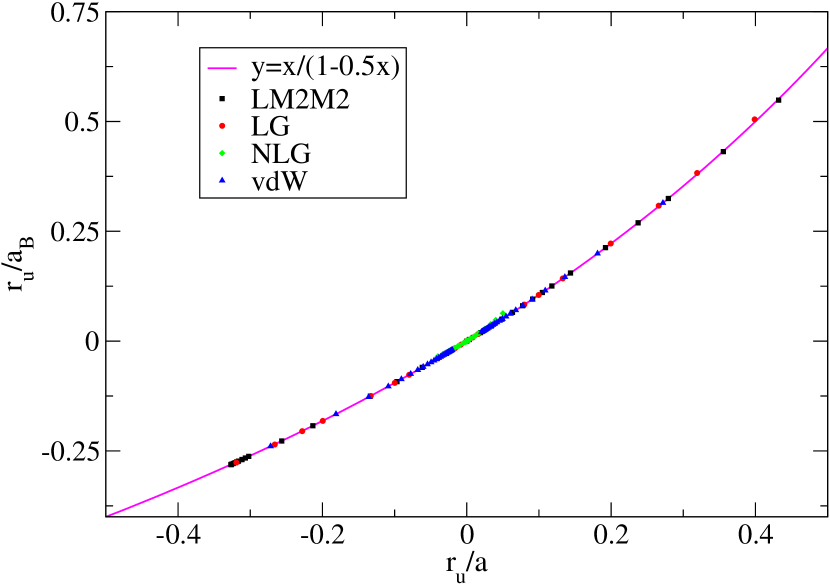
Figure 1: (color online). The relation between the inverse of $a_{B}$ and $a$ (in units of $1/r_{u}$) for the different potential models. All the computed values collapse on the curve $y=x/(1-0.5x)$.

III Universal behavior in the three-body sector

The analysis of the two-boson system indicates that a two-parameter potential as local or non-local gaussian can be used to study the low-energy dynamics around the unitary limit. We will extend the analysis to the three- and four-boson systems. The numerical results for the local gaussian are obtained solving the Schrödinger equation in the coordinate space framework using the Hyperspherical Harmonic expansion XXX1 ; XXX2 ; XXX3 while the predictions for the non-local gaussian are obtained solving Faddeev-Yakubovsky (FY) yakubovsky:67 or Alt-Grassberger-Sandhas (AGS) equations grassberger:67 using momentum-space methods from Refs. deltuva2010 ; deltuva:11a .

The $L=0$ spectrum of three identical bosons in the zero-range limit can be described by the Efimov radial law given in Eq.(1). In the case of a system with a finite range interaction, this equation can be seen as describing the asymptotic spectrum of the three-boson system close to the unitary limit. In fact, the solution of the Schrödinger equation can be used to determine the universal function $\Delta_{3}(\xi)$ looking at the excited states of the spectrum as, for these states, finite-range effects are negligible. In this context the description of few-body systems with potential models close to the unitary limit can be seen as a particular regularization scheme. Accordingly it is possible to modify the Efimov radial law as (see Refs. kievsky2015 ; gatto2014 )

$$E_{3}^{n}/E_{2}=\tan^{2}\xi,$$ (14a)

$$\kappa^{n}_{3}a_{B}=\frac{\text{e}^{-\widetilde{\Delta}^{n}_{3}(\xi)/2s_{0}}}{\cos\xi}\,,$$ (14b)

where $E_{2}=\hbar^{2}/ma_{B}^{2}$ is the dimer binding energy for positive values of $a$ whereas for negative values it is the two-body virtual state energy. Modifications at the three-body level are introduced by the parameters $\kappa^{n}_{3}$ who absorb the scaling factor $e^{n\pi/s_{0}}$ defining the energy of level $n$ at the unitary limit, $E^{n}_{u}=(\hbar^{2}/m)(\kappa^{n}_{3})^{2}$. Furthermore the finite-range character of the interaction slightly modifies the ratio $\kappa^{n}_{3}/\kappa_{3}^{n+1}$ from its universal value of $\approx 22.7$. The main modification in the above equations is the introduction of the level function $\widetilde{\Delta}^{n}_{3}(\xi)$. For the ground state ($n=0$) it could be very different from the zero-range function $\Delta_{3}(\xi)$. As we will see below the differences are much reduced considering the first excited state ($n=1$) and, starting from $n>1$, both functions almost coincide. The level function can be calculated using the corresponding solutions of the Schrödinger equation as

$$\widetilde{\Delta}^{n}_{3}(\xi)=s_{0}\ln\left(\frac{E_{3}^{n}+E_{2}}{E^{n}_{u}}\right).$$ (15)

It should be noticed that for $n=0,1$ this function depends on the particular potential used to calculate the spectrum or, in the case of the STM equation, the cutoff. It depends also on the particular path selected to reach the unitary limit, for example, potentials with variable strength as discussed in the previous section. However, as shown in Ref. kievsky2015 , following this particular path different potentials do not produce too much spread in $\widetilde{\Delta}^{0}_{3}(\xi)$ and $\widetilde{\Delta}^{1}_{3}(\xi)$. Furthermore the LG potential defines a unique gaussian function $\widetilde{\Delta}^{n}_{3}(\xi)$ for each level $n$ independent of the range, $r_{0}$, of the potential. In particular, for the first two levels $n=0,1$, the binding momenta at the unitary limit are $\kappa_{3}^{0}=0.4874/r_{0}$ and $\kappa_{3}^{1}=0.0212/r_{0}$ and the ratio $\kappa_{3}^{0}/\kappa_{3}^{1}\approx 23.0$. These values have been obtained with the potential acting only in $s$-waves, they are slightly different when the LG potential is taken to act in all waves (see for example Refs. kievsky2013 ; kievsky2015 ). Also the NLG potential acting in $s$-wave defines a unique nonlocal gaussian function with the following universal ratios $\kappa_{3}^{0}/k_{0}=0.2127$, $\kappa_{3}^{1}/k_{0}=0.009085$ and $\kappa_{3}^{0}/\kappa_{3}^{1}\approx 23.4$. From the above discussion the following picture emerges: a two-parameter potential as the local or nonlocal gaussians can be used to construct level functions for each level $n$ of the three-boson system. For $n=0,1$ these functions are different from the zero-range universal function and are also different among themselves. For $n>1$ they converge to the zero-range universal function showing a universal behavior. In order to analyze this fact quantitatively, in Fig. 2 the level functions $\widetilde{\Delta}^{0}_{3}(\xi)$ and $\widetilde{\Delta}^{1}_{3}(\xi)$ are shown for the case of the LG, NLG and LM2M2 potentials. The trend discussed above is visible in the figure, for the ground state the level functions $\widetilde{\Delta}^{0}_{3}(\xi)$ spread in a narrow band and are rotated with respect to the universal function $\Delta_{3}(\xi)$, given by the red solid curve hammer2016 . In the case of the first excited state the level functions $\widetilde{\Delta}^{1}_{3}(\xi)$ spread also in a very narrow band very close to $\Delta_{3}(\xi)$. The level function $\widetilde{\Delta}^{3}_{3}(\xi)$ calculated using the NLG third excited state (red diamonds) completely overlaps with the zero-range universal function.

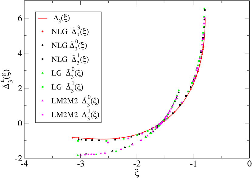
Figure 2: (color online). The level functions $\widetilde{\Delta}^{n}_{3}(\xi)$ for different levels and potentials. The zero-range universal function $\Delta_{3}(\xi)$ is shown as the red solid curve.

The Efimov radial law is a one-parameter equation. The knowledge of the universal function $\Delta_{3}(\xi)$ allows for a complete determination of the spectrum after assigning a value to $\kappa_{*}$ (or to one of the energies $E_{3}^{n}$). Eq.(14) applies mostly to $n=0,1$ and works slightly differently. In first place it is necessary to calculate the level functions for the ground and first excited state. This can be done using for example the LG or NLG potentials. At this point the equation is a one-parameter equation and the $n=0$ and $n=1$ spectrum can be completely determined from the knowledge of one energy. One can argue that if we use Eq.(14) to describe a particular system, the respective potential could be used to compute the level function $\widetilde{\Delta}^{0}_{3}(\xi)$ or $\widetilde{\Delta}^{1}_{3}(\xi)$ by varying the strength in order to reach the unitary limit. However, as it is shown in Fig. 2, close to the unitary limit the three-boson system has universal behavior and therefore a two-parameter potential captures the essential ingredients of the dynamics absorbing finite range effects. As an example we can use $\widetilde{\Delta}_{0}(\xi)$ computed using the LG or NLG potentials to estimate the three-body parameter $\kappa^{0}_{3}$ of a system composed by three ⁴He atoms. As given in Ref. kievsky2015 the result using the LG potential is $\kappa^{0}_{3}\approx 0.0438\;$a${}_{0}^{-1}$ (a${}_{0}=0.529177\ldots\;$ Å  is the Bohr radius). Using the NLG we obtain $\kappa^{0}_{3}\approx 0.0442\;$a${}_{0}^{-1}$ whereas with the LM2M2 potential the result is $0.0440\;$a${}_{0}^{-1}$. This shows that the level functions produce a description with the accuracy better than $1\%$ . The results for the three-body parameter corresponding to the first excited state are $\kappa^{1}_{3}\approx 0.0018\;$a${}_{0}^{-1}$ and $\kappa^{1}_{3}\approx 0.0019\;$a${}_{0}^{-1}$ for the LG and NLG respectively. To be compared to the LM2M2 value of $\kappa^{1}_{3}=0.0019\;$a${}_{0}^{-1}$. As expected finite range effects are reduced in this level.

IV Universal behavior in the four-body sector

The previous analysis can be extended to the four-body case. In this case a two-level structure, with energies $E_{4}^{n,0}$ and $E_{4}^{n,1}$, is attached to each $E_{3}^{n}$ level platter2004 ; hammer2007 ; green2009 ; hadi2011 . As in the three-body case, the four-body system can be studied using potential models, also in this case there is a modification of the universal ratios due to finite-range effects (see for example Refs. deltuva:11a ; kievsky2014 ). Following the previous discussion, the equations describing the four-boson spectrum can be written as

$$E_{4}^{n,m}/E_{2}=\tan^{2}\xi\;\;,$$ (16a)

$$\kappa^{n,m}_{4}a_{B}=\frac{\text{e}^{-\widetilde{\Delta}^{n,m}_{4}(\xi)/2s_{0}}}{\cos\xi}\,.$$ (16b)

with $m=0,1$ and $n$ identifying the corresponding three-body branch. The four-body parameters $\kappa^{n,m}_{4}$ are related to the energy of the level at the unitary limit, $E^{n,m}_{u}=\hbar^{2}(\kappa_{4}^{n,m})^{2}/m$. It should be stressed that only the branch $n=0$, with energies $E_{4}^{0,0}$ and $E_{4}^{0,1}$, corresponds to true bound states. The other states, corresponding to branches with $n>0$, are above the trimer ground state threshold and therefore are unstable bound states (UBS) deltuva:11a ; kok . In the above equation we have introduced the level function $\widetilde{\Delta}^{n,m}_{4}(\xi)$ that governs the four-body spectrum in levels $n,m$. They can be computed using potential models using the following definition

$$\widetilde{\Delta}^{n,m}_{4}(\xi)=s_{0}\ln\left(\frac{E_{4}^{n,m}+E_{2}}{E^{n,m}_{u}}\right)\;.$$ (17)

For $n=0$ it could be very different from the universal function $\Delta^{m}_{4}(\xi)$ that governs the four-body spectrum in the zero-range limit. However, as $n$ increases finite-range effects become negligible and $\widetilde{\Delta}^{n,m}_{4}(\xi)$ should tend to that function. The results are shown in Fig. 3 where the function $\widetilde{\Delta}^{n,m}_{4}(\xi)$ has been calculated using the LG and NLG potentials for the ground state, $n=0,m=0$ level (squares) and first excited state, $n=0,m=1$ level (triangles). For the sake of comparison the function corresponding to the $n=3,m=0$ level (circles) and calculated using the NLG is also shown. From the figure we can see that the results of both potentials for the $n=0,m=0$ and $n=0,m=1$ levels are close to each other. However there is a difference between the functions with different $m$ values, more pronounced for $\xi<-\pi/2$.

Eq.(16) works very similar to the three-body case discussed before. The knowledge of $\widetilde{\Delta}^{n,m}_{4}(\xi)$ makes this equation a one parameter equation. We would like to stress that $\widetilde{\Delta}^{n,m}_{4}(\xi)$ can be computed using a LG or a NLG potential and then used to determine the spectrum of a real system around the unitary limit. As an example we discuss the spectrum of four He atoms. A very complete discussion of this system has been given in Refs.hiyama2012 ; hiyama2014 using realistic potentials. The binding energies of the tetramers using the LM2M2 interaction are $E^{0,0}_{4}=559.22\;$mK and $E^{0.1}_{4}=127.42\;$mK. The dimer energy is $E_{2}=1.3094\;$mK and, therefore the angles are $\xi=-1.52244$ and $-1.46977$ respectively. Using the NLG $\widetilde{\Delta}^{n,m}_{4}(\xi)$ function we estimate $E_{u}^{0,0}\approx 0.443\;$K and $E_{u}^{0,1}\approx 0.0865\;$K in a very good agreement with the quoted values for the LM2M2 potential of $E_{u}^{0,0}\approx 0.4449\;$K and $E_{u}^{0,1}\approx 0.0870\;$K given in Ref. hiyama2014 . We can conclude that the estimates obtained using the level functions are given with an accuracy well below $1\%$.

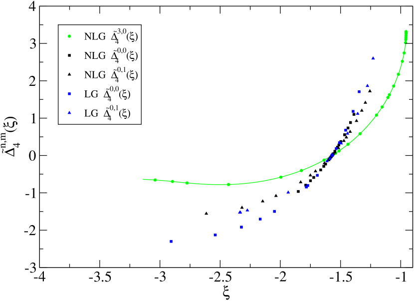
Figure 3: (color online). The level functions $\widetilde{\Delta}^{n,m}_{4}(\xi)$ for different levels and potentials. The solid green line is an interpolation of the $\widetilde{\Delta}^{3,0}_{4}(\xi)$ values and should represent the universal function $\Delta_{4}^{0}(\xi)$.

In Fig. 3 the level function $\widetilde{\Delta}^{3,0}_{4}(\xi)$, calculated using the NLG potential, is shown (circles). For this level finite-range effects can be neglected and, therefore, we can consider this function a good representation of the zero-range four-body universal function in the level $m=0$. For a generic level $m$ we define this function $\Delta_{4}^{m}(\xi)$. It does not depend on the three-body branch $n$, as DSI, with the geometrical factor $e^{\pi/s_{0}}\approx 22.7$, has been already verified among these branches green2009 ; deltuva2010 ; deltuva2012 . In the following we study its dependence on the levels $m$ and its relation with the three-boson universal function $\Delta_{3}(\xi)$. To this aim the level functions $\widetilde{\Delta}^{3,0}_{4}(\xi)$ and $\widetilde{\Delta}^{3,1}_{4}(\xi)$, calculated using the NLG potential, are shown in Fig. 4 together with the zero-range universal function $\Delta_{3}(\xi)$ and the level function $\widetilde{\Delta}^{3}_{3}(\xi)$. We consider $\widetilde{\Delta}^{3}_{3}(\xi)$ a representation of the zero-range universal function $\Delta_{3}(\xi)$ and we consider $\widetilde{\Delta}^{3,m}_{4}(\xi)$ a representation of $\Delta_{4}^{m}(\xi)$. For the $m=1$ case the range of $\xi$ values in which this level results an inelastic virtual state (IVS) is explicitly shown. From the figure we can see that $\Delta_{3}(\xi)$ and $\Delta_{4}^{m}(\xi)$ are very close to each other around the unitary limit. As the functions approach the different thresholds differences appear. In the case of the threshold at $\xi=-\pi$ we have $\Delta_{4}^{0}(-\pi)=\Delta_{4}^{1}(-\pi)=-0.645$, appreciably different from $\Delta_{3}(\xi)=-0.8266$. Defining $a^{n,m}_{4,-}$, the two-body scattering length at which the four-boson system disappears into the four-body continuum, the first relation establishes that

$$\kappa_{4}^{n,m}a^{n,m}_{4,-}=1.378$$ (18)

is a universal number. Defining $a^{n}_{3,-}$ to be the two-body scattering length at which the trimer disappears into the three-body continuum, the second relation results

$$\kappa_{3}^{n}a^{n}_{3,-}=1.508,$$ (19)

confirming the highly accurate value given in Ref. aminus . Within the zero-range theory, the set of values at which the different branches disappear into the three- and four-body continumm can be determined from the above relations using the universal ratios deltuva2012 $a^{n+1}_{3,-}/a^{n}_{3,-}=22.694$, $a^{n,0}_{4,-}/a^{n}_{3,-}=0.4254$, $a^{n,1}_{4,-}/a^{n}_{3,-}=0.9125$.

The dimer-dimer threshold is defined by $\tan\xi_{c}=-\sqrt{2}$ corresponding to $\xi_{c}=-0.9553$. In Fig. 4 we can observe that around this value $\Delta^{0}_{4}(\xi)$ differs from $\Delta^{1}_{4}(\xi)$ and $\Delta_{3}(\xi)$, with these last two functions close to each other. It should be noticed that in this region $\Delta^{1}_{4}(\xi)$ is obtained from the energy of the IVS except for the vicinity of $\xi_{c}$ where the shallow tetramer again becomes UBS before decaying through the dimer-dimer threshold. The values of the universal functions at the critical value $\xi_{c}$ can be calculated using the universal ratios of Ref. deltuva:11b : $a^{n,0}_{dd}/a^{n}_{dd}=0.3235$, $a^{n,1}_{dd}/a^{n}_{dd}=0.99947$, $a^{n}_{dd}/a^{n}_{d}=6.789$ and the relation $\kappa^{n}_{3}a_{n}^{d}=0.0707645$, with $a^{n,m}_{dd}$, $a^{n}_{dd}$ and $a_{n}^{d}$ the scattering lengths at which the level $n,m$ of the tetramer intersects the dimer-dimer threshold and at which the level $n$ of the trimer intersects the dimer-dimer and dimer thresholds, respectively. Using these ratios in Eq.(16) it results $\Delta^{0}_{4}(\xi_{c})=3.316$ and $\Delta^{1}_{4}(\xi_{c})=2.580$, respectively, in complete agreement with the computed values shown in Fig. 4. We can conclude that the small differences between $\Delta^{0}_{4}(\xi)$ and $\Delta^{1}_{4}(\xi)$ around the critical value are due to threshold effects.

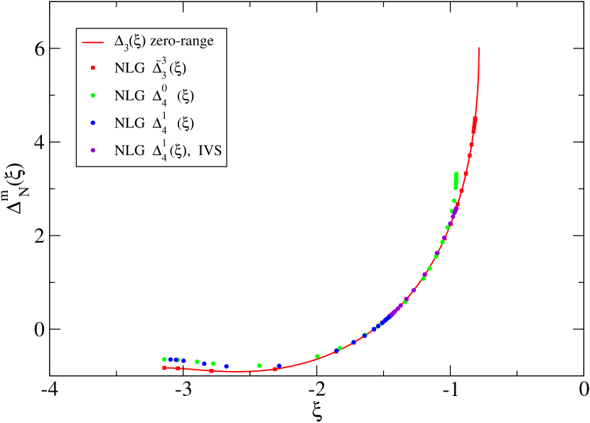
Figure 4: (color online). The universal functions $\Delta^{0}_{4}(\xi)$ (green solid points) and $\Delta^{1}_{4}(\xi)$ (blue solid points and violet solid points in the IVS region). For the sake of comparison, the three-boson universal function $\Delta_{3}(\xi)$ and level function $\Delta^{3}_{3}(\xi)$ are also shown.

From the above discussion we propose the following zero-range equation for the $L=0$ spectrum of four equal bosons

$$E_{4}^{n,m}/(\hbar^{2}/ma^{2})=\tan^{2}\xi$$ (20a)

$$\kappa_{*}^{m}a=\text{e}^{(n-n^{*})\pi/s_{0}}\frac{\text{e}^{-\Delta_{4}^{m}(\xi)/2s_{0}}}{\cos\xi}\,,$$ (20b)

with $\kappa_{*}^{m}$ the binding momentum of the level $n_{*},m$ at the unitary limit verifying the following universal ratio $\kappa_{*}^{0}/\kappa_{*}^{1}=2.1449$ and $\Delta_{4}^{m}(\xi)$ the universal four-boson universal function given in Fig. 4. This equation extends the Efimov radial law for three bosons to the four-boson system.

V Conclusions

In the present work we have analysed two-, three- and four-boson systems close to the unitary limit. To this aim we have solved the Schrödinger equation (or FY and AGS equations) using potential models with variable strength constructed to reproduce the minimal information given by the two-body scattering length $a$ and the two-body binding energy or virtual state energy $E_{2}$. It has been shown that a two-parameter interaction as a gaussian can capture the main ingredients of the dynamics in this region. Moreover these type of potentials define level functions independent of the range used to compute it. This property can be used to construct level functions of general validity that can be used to predict some characteristics of real systems along the particular path used to reach the unitary limit. The level functions $\widetilde{\Delta}_{3}^{n}$ and $\widetilde{\Delta}_{4}^{n,m}$ have two properties: when they are used in the lowest branches, $n=0,1$, they absorb finite-range effects. This portion of the spectrum does not show a perfect DSI since finite-range effects are visible. So the interest here is to use the level functions to describe the dynamics of real systems close to the unitary limit. For example potentials with variable strength describe with reasonable accuracy the variation of the interatomic potential using broad Feshbach resonances in ultra cold atomic traps.

The second property is given by the description of the asymptotic part of the spectrum. For levels with $n>1$ the spectrum calculated with the potentials starts to show DSI and coincides with the spectrum in the zero-range limit. Accordingly, the level functions for $n>1$ do not depend any more on the level number $n$ and on the particular potential used to compute it as well as the path selected to reach the unitary limit. They are good representations of the universal functions $\Delta_{3}$ and $\Delta_{4}^{m}$. This property has been used here to propose Eq.(20) as an extension of the Efimov radial law for four bosons.

In the present work we have studied a particular path to reach the unitary limit based on a single channel potential with variable strength. Other possibilities could be for example the study of coupled channel interactions as in molecular systems. In this way different level functions can be constructed allowing to a systematic study of finite-range effects. Other improvements of the present work could be the study of the spectrum as the number of bosons increases. Preliminary results along this line have been obtained kievsky2014 . Finally we would like to mention the recent study of Efimov physics in the three-body system having spin-isospin degrees of freedom kievsky2016 . The extension to the four-body system is under way.

- (1) V. Efimov, Phys. Lett. B 33, 563 (1970)
- (2) V. Efimov, Sov.J. Nucl. Phys. 12, 589 (1971),
- (3) T. Kraemer et al., Nature 440, 315 (2006)
- (4) F. Ferlaino, A. Zenesini, M. Berninger, B. Huang, H.C. Nägerl, and R. Grimm, Few-Body Syst. 51, 113 (2011)
- (5) O. Machtey, Z. Shotan, N. Gross, and L. Khaykovich, Phys. Rev. Lett. 108, 210406 (2012)
- (6) S. Roy, M. Landini, A. Trenkwalder, G. Semeghini, G. Spagnolli, A. Simoni, M. Fattori, M. Inguscio, and G. Modugno, Phys. Rev. Lett. 111, 053202 (2013)
- (7) P. Dyke, S.E. Pollack, and R.G. Hulet, Phys. Rev. A 88, 023625 (2013)
- (8) P.F. Bedaque, H.-W. Hammer, and U. van Kolck, Phys. Rev. Lett.82, 463 (1999)
- (9) P. Bedaque, H.-W. Hammer, and U. van Kolck, Nucl. Phys. A676, 357 (2000)
- (10) E. Braaten and H.-W. Hammer, Phys. Rep. 428, 259 (2006)
- (11) T. Frederico, L. Tomio, A. Delfino, M. R. Hadizadeh, and M.T. Yamashita, Few-Body Syst. 51, 87 (2011)
- (12) L.H. Thommas, Phys. Rev. 47, 903 (1935)
- (13) E. Braaten, H.-W. Hammer and M. Kusunoki, Phys. Rev. A 67, 022505 (2003)
- (14) L. Platter, H.W. Hammer, and Ulf-G. Meißner, Phys. Rev. A70, 052101 (2004)
- (15) H.-W Hammer and L. Platter, Eur. Phys. J. A32, 113 (2007)
- (16) J, von Stecher, J.P. D’Incao abd C.H. Greene, Nat. Phys. 5, 417 (2009)
- (17) M. R. Hadizadeh, M.T. Yamashita, L. Tomio, A. Delfino, and T. Frederico, Phys. Rev. Lett. 107, 135304 (2011)
- (18) A. Deltuva, Phys. Rev. A82, 040701(R) (2010)
- (19) A. Kievsky and M. Gattobigio, Phys. Rev. A 92, 062715 (2015)
- (20) C. Chin, R. Grimm, P. Julienne and E. Tiesinga, Rev. Mod. Phys. 82, 1225 (2010)
- (21) R.A. Aziz and M.J. Slaman, J. Chem. Phys. 94, 8047 (1991)
- (22) A. Kievsky, L.E. Marcucci, S. Rosati and M. Viviani, Few-Body Syst. 22, 1 (1997)
- (23) M. Viviani, A. Kievsky and S. Rosati, Phys. Rev.C71, 024006 (2005)
- (24) M. Gattobigio, A. Kievsky and M. Viviani, Phys. Rev. A 84, 052503 (2011)
- (25) O. A. Yakubovsky, Yad. Fiz. 5, 1312 (1967) [Sov. J. Nucl. Phys. 5, 937 (1967)].
- (26) P. Grassberger and W. Sandhas, Nucl. Phys. B2, 181 (1967); E. O. Alt, P. Grassberger, and W. Sandhas, JINR report No. E4-6688 (1972).
- (27) A. Deltuva, EPL 95, 43002 (2011).
- (28) M. Gattobigio and A. Kievsky, Phys. Rev. A 90, 012502 (2014)
- (29) A. Kievsky and M. Gattobigio, Phys. Rev. A 87, 052719 (2013)
- (30) H.-W. Hammer, M. Gattobigio and A. Kievsky, in preparation
- (31) A. Kievsky, N.K. Timofeyuk and M. Gattobigio, Phys. Rev. A 90, 032504 (2014)
- (32) A.M. Badalyan, L.P. Kok, M.I. Polikarpov and Y.A. Simonov, Phys. Rep. 82, 31 (1982)
- (33) A. O. Gogolin, C. Mora, and R. Egger, Phys. Rev. Lett. 100, 140404 (2008)
- (34) E. Hiyama and M. Kamimura, Phys. Rev. A 85, 062505 (2012)
- (35) E. Hiyama and M. Kamimura, Phys. Rev. A 90, 052514 (2014)
- (36) A. Deltuva. Phys. Rev. A 85, 012708 (2012)
- (37) A. Deltuva, Phys. Rev. A 84, 022703 (2011).
- (38) A. Kievsky and M. Gattobigio, Few-Body Syst. 57, 217 (2016)