How Violent are the Collisions of Different Sized Droplets in a Turbulent Flow?

Abstract

We study the typical collisional velocities in a polydisperse suspension of droplets in two and three-dimensional turbulent flow and obtain precise theoretical estimates of the dependence of the impact velocity of particles-pairs on their relative sizes. These analytical results are validated against data from our direct numerical simulations. We show that the impact velocity saturates exponentially with the inverse of the particle-size ratios. Our results are important to model coalescence or fragmentation (depending on the impact velocities) and will be crucial, for example, in obtaining precise coalescence kernels to describe the growth of water droplets which trigger rain in warm clouds.

A wide variety of industrial, experimental and natural phenomena – such as volcanic eruptions, embryonic planetesimals in circumstellar disks and growth of water droplets triggering rain in warm clouds – involves coalescence, collisions, and fragmentation of small, heavy particles carried by a turbulent flow intro-ref . Given the ubiquitousness and generality of particle-laden flows, problems of this class have been the subject of intense research in the last few years. As a result significant progress has been made in our understanding of not only the appropriate theoretical MR , numerical bec-numerics and mathematical framework bec-math to study such systems but also the nature of coalescence and collisions in both idealised idealised and realistic settings coal . In the last couple of years, for example, several authors have elucidated, theoretically and in experiments, questions related to the distribution of relative velocities of approaching particles  mehlig ; saw and the extreme events associated with them. Such studies are a key building block in helping us to eventually model effective collision kernels which would be crucial in computing, for example, droplet distributions in warm clouds.

Much of the work related to the issue of approach rates and relative velocities of particle-pairs deal with systems of identical particles bec2005 ; bec2010 ; bec2014 . However in nature, the distribution of particles is typically inhomogeneous. Hence particles of different sizes interact with one another. Furthermore, to critically understand if coalescences dominate – leading to the growth of larger and larger droplets – an estimate of the strength of impact velocities of particles with different radii is crucial. In particular the role of preferential concentration (which changes with particle radii) of particles at small scales as well as possible large velocity differences due to caustics caustics and the sling effect sling ought to result in non-trivial collisional velocities in an inhomogeneous size distribution of particles in a turbulent flow.

Given all of this, it behooves us to ask the rate at which droplets or aggregates grow in an inhomogeneous size distribution of particles which are carried by the same turbulent flow. This, it is worth stressing, is the natural setting for processes which are of relevance in nature and in the most general of laboratory settings. A first step in this direction is to understand how violent the impact velocities amongst different particles are in such polydisperse suspensions. A quantitative measure of this, in turn, will suggest whether the impact between particle-pairs of radii $a_{1}$ and $a_{2}$ will result in a coalescence – leading to a larger droplet – or fragmentation frag . Thus, in this paper we address (in two and three dimensions), numerically and theoretically, the critical question of the dependence of the impact velocities of particle-pairs on the relative sizes of the particles.

Dimension	$N$	$N_{p}$	$\nu$	$k_{\rm inj}$	$\eta$	$k_{\rm max}\eta$	$\lambda$	$Re_{\lambda}$	$\tau_{\eta}$
3D	512	$10^{6}$	0.001	1 and 2	0.0059	1.01	0.0856	121	0.0351
2D	1024	$10^{5}$	$10^{-5}$	4	0.0044	1.50	0.20	440	1.92

Table 1: Parameters for our simulations: $N$ is the number of grid points along each direction, $N_{p}$ is the number of Lagrangian and heavy inertial particles, $\nu$ the kinematic viscosity, $\epsilon$ is the fixed energy input, $k_{\rm inj}$ the forcing wavenumber, $\eta\equiv(\nu^{3}/\varepsilon)^{1/4}$ the dissipation scale, $\lambda\equiv\sqrt{\nu E/\varepsilon}$ the Taylor microscale, $Re_{\lambda}\equiv u_{\rm rms}\lambda/\nu$ the Taylor-microscale Reynolds number, and $\tau_{\eta}\equiv\sqrt{\nu/\varepsilon}$ the Kolmogorov time scale.

We consider a fluid flow whose velocity $\bm{u}$ is a solution to the incompressible Navier–Stokes equation

$$\partial_{t}\boldsymbol{u}+(\boldsymbol{u}\cdot\nabla)\boldsymbol{u}=-\nabla p+\nu\nabla^{2}\boldsymbol{u}+\boldsymbol{f},\quad\nabla\cdot\boldsymbol{u}=0,$$ (1)

where $\nu$ designates the fluid kinematic viscosity. In two dimensions (2D), it is often convenient to re-write this in the vorticity ($\omega$)-stream function ($\psi$) formulation prasad as

$$\partial_{t}\omega-J(\psi,\omega)=\nu\nabla^{2}\omega+f_{\omega}-\mu\omega,$$ (2)

where $J(\psi,\omega)\equiv(\partial_{x}\psi)(\partial_{y}\omega)-(\partial_{x}\omega)(\partial_{y}\psi)$ and $\mu$ is the coefficient of Ekman friction. At the point ($x$,$y$) the velocity $\bm{u}\equiv(-\partial_{y}\psi,\partial_{x}\psi)$ and the vorticity $\omega=\nabla\psi$.

We now study the dynamics of small inertial particles (droplets) which are suspended in a turbulent flow field obtained as a solution of Eq. (1) in three dimensions (3D) or of Eq. (2) in 2D in the limit of small $\nu$ or large Reynolds numbers. We assume that our particles are much smaller than the Kolmogorov scale $\eta$, much heavier than the surrounding fluid, and with a small Reynolds number associated to their slip velocity. The motion of the i-th particle, in the turbulent fluid, is damped through a viscous Stokes drag and their trajectories $\boldsymbol{x}_{\mathrm{i}}(t)$ are defined via

$$\frac{\mathrm{d}{\boldsymbol{x}_{\mathrm{i}}}}{\mathrm{d}{t}}=\boldsymbol{v}_{\mathrm{i}},\quad\frac{\mathrm{d}{\boldsymbol{v}_{\mathrm{i}}}}{\mathrm{d}{t}}=-\frac{1}{\tau_{\mathrm{p}}}\left[\boldsymbol{v}_{\mathrm{i}}-\boldsymbol{u}(\boldsymbol{x}_{\mathrm{i}},t)\right].$$ (3)

The relaxation time $\tau_{\mathrm{p}}\!=\!2\rho_{\mathrm{p}}a^{2}/(9\rho_{\mathrm{f}}\nu)$, where $\rho_{\mathrm{p}}$ and $\rho_{\mathrm{f}}$ are the particle and fluid mass density respectively and $a$ the particle radius, allows us to define a non-dimensional Stokes number $St=\tau_{p}/\tau_{\eta}$; the small time-scale $\tau_{\eta}$ is the Kolmogorov time scale and an intrinsic property of the fluid frisch95 .

We perform direct numerical simulations (DNSs) of Eq. (3) coupled with Eq. (1) in 3D or Eq. (2) in 2D. The Navier-Stokes equations are solved in a 2$\pi$ periodic domain (with the number of collocation points $N^{3}$ (3D) or $N^{2}$ (2D)) by using a standard pseudospectral method and a second-order Runge-Kutta scheme for time-marching. We maintain statistically steady homogeneous, isotropic turbulence via the large-scale forcing $\boldsymbol{f}$ in 2D and by a constant energy injection in 3D on wavenumbers $k_{\rm inj}$. The parameters of both sets of simulations are given in Table 1.

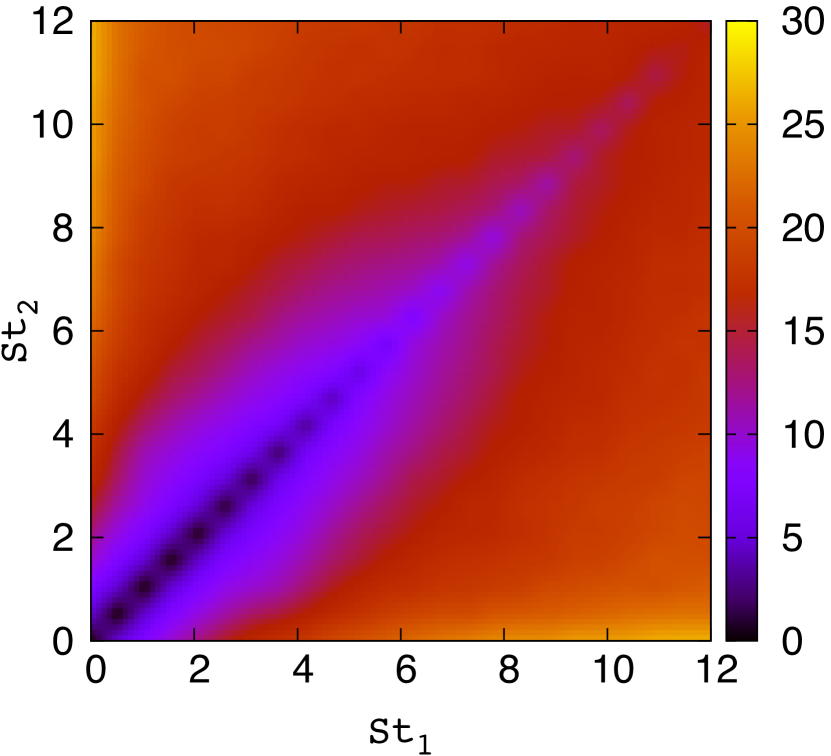
Figure 1: (color online) Impact velocity $\boldsymbol{\Delta}(St_{\mathrm{1}},St_{\mathrm{2}})$ as a function of Stokes numbers of approaching particles in 2D.

We solve Eq. (3) numerically for $N_{p}$ (see Table 1) non-interacting particles associated with a Stokes time $\tau_{p}$; we choose 50 different $\tau_{p}$ in 2D and 20 different $\tau_{p}$ in 3D. We thus integrate individual particle trajectories for different values of $\tau_{\mathrm{p}}$ and the fluid velocity $\bm{u}$ at their location is evaluated by linear interpolation. We study the dynamics of the particles within the framework of ghost collisions and hence we do not perform any real collisions; results of the effect of collisions will be reported elsewhere martin . Given the assumption on the particle sizes, we work within the framework of one-way coupling between the particles and the fluid and ignore any effect of the particles on the flow.

Case	$St_{1}$	$St_{2}$	Prediction	Figure
Case 1	–	$St_{1}$	$\boldsymbol{\Delta}=\boldsymbol{\Delta}_{0}\exp{(-\tau/St)}$	Fig. 2
Case 2	$St_{1}\ll 1$	$St_{2}\lesssim 1$	$\boldsymbol{\Delta}\sim St_{2}$	Fig. 3
Case 3	$St_{1}\ll 1$	$St_{2}\gg 1$	$\boldsymbol{\Delta}=\boldsymbol{\Delta}_{0}\exp{(-\tau/St_{2})}$	Fig. 3
Case 4	$St_{1}\gtrsim 1$	$St_{2}\neq St_{1}$	None	Fig. 4

Table 2: A summary of the different asymptotics and the theoretical predictions for $\boldsymbol{\Delta}$.

The impact velocity between colliding droplets, which determines the chance of coalescence or fragmentation, is defined as the velocity difference of the two particles at vanishing separation. Thence, we define the impact velocity between two particles, labelled 1 and 2, of Stokes numbers $St_{1}$ and $St_{2}$ as $\boldsymbol{\Delta}=\langle|({\bf v}_{2}-{\bf v}_{1})\cdot\hat{\bf r}|\rangle$, where the unit vector $\hat{\bf r}$ defines the vector connecting the centers of the two particles, with the constraint that $({\bf v}_{2}-{\bf v}_{1})\cdot\hat{\bf r}<0$ which define a pair of approaching particles foot1 . The averaging $\langle\cdot\rangle$ is defined over all colliding pairs.

In Fig. 1 we show a pseudo-color plot of the amplitude of the impact velocity $\boldsymbol{\Delta}$ as a function of the Stokes numbers of the colliding particles is shown from our data from the 2D simulations, with similar results obtained in our 3D DNS. (In this plot and all subsequent plots, we show $\boldsymbol{\Delta}$ normalised by the Kolmogorov velocity $u_{\eta}=\eta/\tau_{\eta}$ of the underlying turbulent fluid.) Qualitatively, it is easy to understand the diagonal ($St_{1}=St_{2}$) behaviour of $\boldsymbol{\Delta}$: The two-particle velocity correlation between particles (when the size of one particle is fixed and the other varied) attains a maximum when particles are of the same size ($St_{1}=St_{2}$) Wang . Consequently, $\boldsymbol{\Delta}$ attains a minimum when the approaching particles have the same Stokes number as is clearly seen in Fig. 1. For larger Stokes numbers, $\boldsymbol{\Delta}$ becomes larger because of the formation of caustics which allow same-sized particles to collide with each other with arbitrarily large velocities.

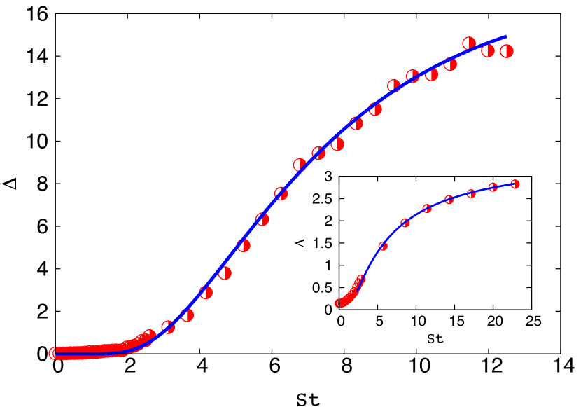
Figure 2: (color online) Plot $\boldsymbol{\Delta}$ as a function of $St$ for same-sized particles. The blue solid curve is our theoretical prediction and the symbols are data from our simulations in 2D and 3D (inset). The error bars on our numerical data are comparable to the symbol size.

In order to gain a complete understanding of the dependence of $\boldsymbol{\Delta}$ on $St_{1}$ and $St_{2}$, it is useful to return to Eq. (3). Let us consider two particles 1 and 2 with Stokes times $\tau_{1}=\tau$ and $\tau_{2}=\alpha\tau_{1}=\alpha\tau$. We consider the non-dimensional form of Eq. (3) (by including factors of $\tau_{\eta}$) to obtain

$$\frac{d{\bf v}_{1}}{d\tau} = -\frac{1}{St}[{\bf v}_{1}-{\bf u}_{1}];$$

$$\frac{d{\bf v}_{2}}{d\tau} = -\frac{1}{\alpha St}[{\bf v}_{2}-{\bf u}_{2}].$$

For brevity, we set $\boldsymbol{u}(\boldsymbol{x}_{\mathrm{i}},t)={\bf u}_{\rm i}$. Thence we obtain

$$\frac{d\boldsymbol{\Delta}}{dt}=-\frac{1}{\alpha St}\left[\boldsymbol{\Delta}-St(1-\alpha)\frac{d{\bf v}_{1}}{dt}\cdot\hat{\bf r}\right].$$ (4)

We have assumed here that at small particle separations $|{\bf r}|$, the fluid velocity is smooth and hence $|{\bf u}_{1}-{\bf u}_{2}|\equiv{\bf\sigma}\cdot{\bf r}\sim 0$, as $|{\bf r}|\to 0$ (${\bf\sigma}$ is the gradient of the fluid velocity).

So far we have made only one defensible assumption in deriving Eq. (4) which has to do with the smoothness of the velocity field at small scales. To this extent Eq. (4) is exact in both 2D and 3D. Let us now explore the various asymptotics of this equation and obtain theoretical estimates of $\boldsymbol{\Delta}$ for different combinations of Stokes numbers which can then be tested against data from our DNSs in 2D and 3D. The following limits naturally arise in this case (see Table 2 for a compact version of these limits): Case 1: $\alpha=1$ with no assumption on $St$; Case 2: Particle 1 is very small and close to being a tracer ($St\ll 1$) and $\alpha\sim\mathcal{O}(1)$ such that $St_{2}\lesssim 1$; Case 3: Particle 1 is still small ($St\ll 1$) but $\alpha\gg 1$ such that $St_{2}\gg 1$; and Case 4: For $St\gtrsim 1$. To obtain the limiting form of $\boldsymbol{\Delta}$ from Eq. (4) in each such case, we assume that at time $t=0$ the particles have come close to each other (without actually colliding) with a velocity difference $\boldsymbol{\Delta}_{0}$ and then, over a time $\tau$, they touch.

For $\alpha=1$ (Case 1), integrating Eq. (4), we obtain $\boldsymbol{\Delta}=\boldsymbol{\Delta}_{0}\exp{(-\tau/St)}$, where (and in what follows) $\boldsymbol{\Delta}_{0}$ is the constant of integration. In Fig. 2 we test our theoretical prediction (solid line) against data from our DNSs (symbols) in both 2D and 3D (inset) and find excellent agreement between the two.

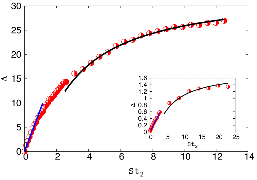
Figure 3: (color online) Representative plot of $\boldsymbol{\Delta}$, shown with symbols from our DNS data, as a function of $St_{2}$ for $St=0.005\ll 1$ in 2D and for tracers in 3D (inset). Our theoretical prediction for $St_{2}<1$ and for $St_{2}\gtrsim 1$ are shown by the blue and black solid curves, respectively. The error bars on our numerical data are comparable to the symbol size.

We now address the important question of what happens when the two colliding particles have different Stokes numbers. Let us begin with Case 2 where $St\ll 1$ ($v_{1}\approx u_{1}$) and $\alpha\sim\mathcal{O}(1)$. In this limit, we can rewrite Eq. (4) as

$$\alpha St\frac{d\boldsymbol{\Delta}}{dt}=-\left[\boldsymbol{\Delta}-St(1-\alpha)\frac{d{\bf v}_{1}}{dt}\cdot\hat{\bf r}\right].$$ (5)

Since $\alpha St<1$, we can set $\alpha St\frac{d\boldsymbol{\Delta}}{dt}=0$ and obtain $\boldsymbol{\Delta}\sim St_{2}$. In the other limit, Case 3, where $St\ll 1$ and $\alpha\gg 1$ such that $\alpha St>1$, we notice that $\frac{St(1-\alpha)}{\alpha St}\frac{d{\bf v}_{1}}{dt}\cdot\hat{\bf r}\sim\frac{d{\bf v}_{1}}{dt}\cdot\hat{\bf r}\sim 0$ to leading order since $St\ll 1$. Thence we obtain $\boldsymbol{\Delta}=\boldsymbol{\Delta}_{0}\exp{(-\tau/St_{2})}$.

Given the strong assumptions made in arriving at the two limits above, it is important to check our prediction against data from our DNSs. In Fig. 3 we show a representative plot of the impact velocity $\boldsymbol{\Delta}$ between particles of Stokes number $St=0.005$ (2D) and tracers (3D, inset) foot2 with particles of different Stokes numbers. We immediately notice that when $St_{2}\lesssim 1$, $\boldsymbol{\Delta}$ is indeed linear with $St_{2}$ and the data (symbols) consistent with our theoretical prediction shown as a blue curve. In the other limit when $St_{2}\gg 1$, our data from numerical simulations is in excellent agreement with the theoretical prediction $\boldsymbol{\Delta}\sim\exp{(-1/St_{2})}$.

At this stage it is important to remark about the constant of integration. $\boldsymbol{\Delta}_{0}$ is the typically velocity difference with which two droplets come near each other. From very general conditions, it is likely that $\boldsymbol{\Delta}_{0}$ should depend on turbulent intensity, the spatial dimension, as well as the relative Stokes numbers of the fluid (when $St_{1},St_{2}\sim\mathcal{O}(1)$. However we do not have an analytical expression for $\boldsymbol{\Delta}_{0}$ and as our theoretical and numerical results suggest, $\boldsymbol{\Delta}_{0}$ is likely to be a constant or an algebraic, sub-dominant prefactor atleast in the range of Stokes numbers studied here foot3 .

Let us finally turn to the situation when $St\gtrsim 1$ (Case 4). In Fig. 4 we show a representative plot of the impact velocity between a particle of Stokes number $St=12.5$ (2D) and $St=20$ (3D, inset) with all other particles. From our numerical data we see that that $\boldsymbol{\Delta}$ shows rapid variation when $St_{2}\lesssim St_{1}$. However we do not have a self-consistent understanding of the functional form of the decrease in $\boldsymbol{\Delta}$ from Eq. (4).

Before concluding, we return to theoretical considerations which are central to this study. In recent years much work has gone into understanding how large particle aggregates are formed – mainly through coalescence – from small nuclei particles carried in a turbulent flow. This question is of fundamental importance when tackling issues as diverse as formation of large rain droplets in warm clouds, pollutant dispersion and concentration, and the growth of planetesimals in astrophysics. A stumbling block in a fully self-consistent theory to explain such accelerated growths is the lack of realistic collision-coalescence kernels for different-sized particles which incorporate both fragmentation and coalescence. A first step in this direction is, of course, determining the dependence of impact velocities of colliding particles on their sizes. In this paper we show, through theory and simulations, what this dependence is.

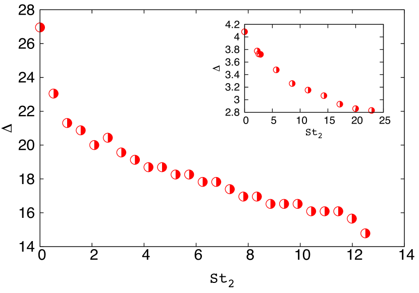
Figure 4: (color online) Representative plot of $\boldsymbol{\Delta}$ for $St=12.5\gg 1$ in 2D and for $St=20\gg 1$ in 3D (inset) from our numerical simulations (symbols) as a function of $St_{\mathrm{2}}$. The error bars on our numerical data are comparable to the symbol size.

Our results, summarised in Table 2, are remarkable in their implication. We show that the larger particles (large Stokes numbers) do not collide with arbitrarily large velocities with the smaller, tracer-like particles but actually saturate ($\sim\exp{(-1/St)}$). This suggests that in inhomogeneous suspensions, such as the polydisperse droplet distribution in warm clouds, a run-away growth for large droplets through coalescence (and not fragmenting because of large velocity differences) is likely to be the dominant mechanism triggering rain coal ; wilkinson .

In conclusion, we have developed a systematic theory, validated through detailed numerical simulations, for the impact velocity of colliding droplets of different sizes. Remarkably, our results seem to be independent of dimension. In particular we have shown that there is a limiting form for the impact velocity and hence in natural settings coalescence – and not fragmentation due to large $\boldsymbol{\Delta}$ – should be the dominant mechanism. Therefore this work is a significant step in developing models for coalescing droplets. Important questions related to Reynolds and Froude number effects is beyond the scope of the present work and the issue of collision frequencies in polydisperse suspensions is addressed elsewhere martin .

- (1) S. Weidenschilling and J. N. Cuzzi, in Protostars and Planets III, Vol. 1 (1993) pp. 1031-1060; J. J. Lissauer, Ann. Rev. Astron. Astrophys. 31, 129 (1993); M. Pinsky and A. Khain, J. Aerosol Sci. 28, 1177 (1997); R. Shaw, Annu. Rev. Fluid Mech. 35, 183 (2003).
- (2) M. R. Maxey and J. J. Riley, Phys. Fluids 26, 883-889 (1983).
- (3) J. Bec, et al. J. Fluid Mech. 550, 349-358, (2006); M. Cencini, et al., J. Turbul. 7, 1-16, (2006); J. Bec et al., Phys. Rev. Lett. 98, 084502, (2007).
- (4) J. Bec, Phys. Fluids 15, L81-L84 (2003); J. Bec, M. Cencini and R. Hillerbrand, Physica D 226, 11-22, (2007); J. Bec, M. Cencini and R. Hillerbrand, Phys. Rev. E 75, 025301, (2007).
- (5) J. Bec, J. Fluid Mech. 528, 255-277, (2005); J. Bec, S. Musacchio and S. S. Ray, Phys. Rev. E 87 063013, (2013).
- (6) J. Bec, S. S. Ray, E. W. Saw and H. Homann, arXiv:1507.02034 (2015).
- (7) E.-W. Saw, G.P. Bewley, E. Bodenschatz, S. S. Ray and J. Bec, Phys. Fluids 26, 111702, (2014).
- (8) K. Gustavsson and B. Mehlig, Phys. Rev. E 84, 045304 (2011); K. Gustavsson and B. Mehlig, J. Turbul. 15, 34-69 (2013).
- (9) J. Bec, A. Celani, M. Cencini, and S. Musacchio, Phys. Fluids 17, 073301 (2005).
- (10) J. Bec, L. Biferale, M. Cencini, A. Lanotte, and F. Toschi, J. Fluid Mech. 646, 527 (2010).
- (11) J. Bec, H. Homann, and S. S. Ray, Phys. Rev. Lett. 112, 184501, (2014).
- (12) M. Wilkinson, B. Mehlig, and V. Bezuglyy, Phys. Rev. Lett. 97, 048501 (2006).
- (13) G. Falkovich, A. Fouxon, and M. G. Stepanov, Nature 419, 151 (2002).
- (14) M. Orme, Prog. Energy Combust. Sci. 23, 65-79 (1997).
- (15) P. Perlekar, S. S. Ray, D. Mitra, and R. Pandit, Phys. Rev. Lett. 106, 054501 (2011); S. S. Ray, D. Mitra, P. Perlekar, and R. Pandit, Phys. Rev. Lett. 107, 184503 (2011).
- (16) U. Frisch, Turbulence the Legacy of A.N. Kolmogorov (Cambridge Universite Press, Cambridge, England, 1996).
- (17) M. James and S. S. Ray, manuscript in preparation (2016).
- (18) We note that the same definition can be arrived at by considering the velocity longitudinal structure function calculated in the limit where the pair separation goes to 0.
- (19) Y. Zhou, A. S. Wexler, and L.-P. Wang, Phys. Fluids 10, 1206 (1998).
- (20) For the 3D simulations, we choose tracers for the reference particle; our theoretical predictions can be shown to hold in the case when as well.
- (21) For droplets which are large, it is plausible that bec2010 .
- (22) M. Wilkinson, Phys. Rev. Lett. 116, 018501 (2016).