Static and rotating universal horizons and black holes in gravitational theories with broken Lorentz invariance

Abstract

In this paper, we show the existence of static and rotating universal horizons and black holes in gravitational theories with broken Lorentz invariance. We pay particular attention to the ultraviolet regime, and show that universal horizons and black holes exist not only in the low energy limit but also at the ultraviolet energy scales. This is realized by presenting various static and stationary exact solutions of the full theory of the projectable Hořava gravity with an extra U(1) symmetry in (2+1)-dimensions, which, by construction, is power-counting renormalizable.

I Introduction

Lorentz invariance (LI) has been the cornerstone of modern physics and is strongly supported by observations Kostelecky:2008ts . In fact, all the experiments carried out so far are consistent with it, and there is no evidence to show that such a symmetry needs to be broken at a certain energy scale, although it is arguable that the constraints in the matter sector are much stronger than those in the gravitational sector M-L .

Nevertheless, there are various reasons to construct gravitational theories with broken LI. In particular, when spacetime is quantized, as what we currently understand from the point of view of quantum gravity Carlip ; Kiefer , space and time emerge from some discrete substratum. Then, LI, as a continuous spacetime symmetry, cannot apply to such discrete space and time any more. Therefore, it cannot be a fundamental symmetry, but instead an emergent one at the low energy physics. Following this line of thinking, various gravitational theories that violate LI have been proposed, such as ghost condensation ArkaniHamed:2003uy , Einstein-aether theory TJ , and more recently, Hořava theory of gravity Horava . While the ghost condensation and Einstein-aether theory are considered as the low energy effective theories of gravity, the Hořava gravity is supposed to be ultraviolet (UV) complete Horava . In particular, in this theory the LI is broken in the UV, so the theory can include higher-dimensional spatial derivative operators. As a result, the UV behavior of the theory is dramatically improved and can be made power-counting renormalizable. On the other hand, the exclusion of higher-dimensional time derivative operators prevents the ghost instability, whereby the unitarity problem of the theory, known since 1977 Stelle:1976gc , is resolved. In the infrared (IR), the lower dimensional operators take over, whereby a healthy low-energy limit is presumably resulted Horava:2011gd . Recently, it was shown that the Hořava theory is not only power-counting renormalizable but also perturbatively renormalizable Barvinsky:2015kil . In addition, it is also very encouraging that the theory is canonically quantizable in (1+1)-dimensional spacetimes with Lia or without Lib the projectability condition.

However, once LI is broken different species of particles can travel with different velocities, and in certain theories, including the Hořava theory mentioned above, they can be even arbitrarily large. This suggests that black holes may exist only at low energies Wang:2012nv . At high energies, any signal initially trapped inside the horizon may be able to escape out of it and propagate to infinity, as long as the signal has sufficiently large velocity (or energy). This seems in a sharp conflict with current observations that support the existence of rotating black holes in our universe Narayan .

The above situation was dramatically changed in 2011 Blas:2011ni ; Barausse:2011pu , in which it was found that there still exist absolute causal boundaries, the so-called universal horizons, and particles even with infinitely large velocities would just move around on these boundaries and cannot escape to infinity. The main idea is as follows. In a given spacetime, a globally timelike scalar field, the so-called khronon Blas:2011ni , might exist. Then, similar to the Newtonian theory, this khronon field defines a global absolute time, and all particles are assumed to move along the increasing direction of the khronon, so the causality is well defined [Cf. Fig. 1]. In such a spacetime, there may exist a surface as shown in Fig. 2, denoted by the vertical solid line. Given that all particles move along the increasing direction of the khronon, from Fig. 2 it is clear that a particle must cross this surface and move inward, once it arrives at it. This is an one-way membrane, and particles even with infinitely large speed cannot escape from it, once they are trapped inside it. So, it acts as an absolute horizon to all particles (with any speed), which is often called the universal horizon Blas:2011ni ; Barausse:2011pu . Since then, this subject has already attracted lots of attention Bhattacharyya:2015uxt .

Figure 1: (a) The light cone of the event $p$ in special relativity. (b) The causal structure of the point $p$ in Hořava theory.

Figure 2: Illustration of the bending of the $\phi$ = constant surfaces, and the existence of the universal horizon in the Schwarzschild spacetime Lin:2014eaa , where $\phi$ denotes the khronon field, and $t$ and $r$ are the Painlevé-Gullstrand coordinates. Particles move always along the increasing direction of $\phi$. The Killing vector $\zeta^{\mu}=\delta^{\mu}_{t}$ always points upward at each point of the plane. The vertical dashed line is the location of the Killing horizon, $r=r_{KH}$. The universal horizon, denoted by the vertical solid line, is located at $r=r_{UH}$, which is always inside the Killing horizon.

However, in most studies of universal horizons carried out so far the khronon plays a part of the gravitational theory involved Bhattacharyya:2015uxt . To generalize the conception of the universal horizons to any gravitational theory with broken LI, recently we considered the khronon as a test field, and assumed it to play the same role as a Killing vector, so its existence does not affect the spacetime considered, but defines the properties of it Lin:2014ija . By this way, such a field is no longer part of the gravitational theory and it may or may not exist in a given spacetime, depending on the spacetime considered. Then, we showed that the universal horizons indeed exist, by constructing concrete static charged solutions of the Hořava gravity. Taking the khronon field as a test field, we further showed that the universal horizons exist and are always inside the Killing horizons Lin:2014eaa in the three well-known black hole solutions: the Schwarzschild, Schwarzschild anti-de Sitter, and Reissner-Nordström. It should be noted that these solutions are often also solutions of gravitational theories with the broken LI, such as the Hořava theory GLLSW , and the Einstein-aether theory TJ .

At the universal horizon, a slightly modified first law of black hole mechanics exists for the neutral Einstein-aether black holes Berglund:2012bu , but for the charged Einstein-aether black holes, such a first law is still absent Ding:2015kba . Using the tunneling method, the Hawking radiation at the universal horizon for a scalar field that violates the local LI was studied, and found that the universal horizon radiates as a blackbody at a fixed temperature Berglund:2012fk . A different approach was taken in Cropp:2013sea , in which ray trajectories in such black hole backgrounds were studied, and evidence was found, which shows that Hawking radiation is associated with the universal horizon, while the “lingering” of low-energy ray trajectories near the Killing horizon hints a reprocessing there. However, the study of a collapsing null shell showed that the mode passing across the shell is adiabatic at late time Michel:2015rsa . This implies that large black holes emit a thermal flux with a temperature fixed by the surface gravity of the Killing horizon. This, in turn, suggests that the universal horizon should play no role in the thermodynamic properties of these black holes, although it should be noted that in such a setting, the khronon field is not continuous across the collapsing null shell. As mentioned above, a globally-defined khronon plays an essential role in the existence of a universal horizon, so it is not clear how the results presented in Michel:2015rsa will be affected once the continuity of the khronon field is imposed. On the other hand, using the Hamilton-Jacobi method, recently we studied quantum tunneling of both relativistic and non-relativistic particles at Killing as well as universal horizons of Einstein-Maxwell-aether black holes, after higher-order curvature corrections are taken into account Ding:2015fyx . Our results showed that only relativistic particles are created at the Killing horizon, and the corresponding radiation is thermal with a temperature exactly the same as that found in general relativity. In contrary, only non-relativistic particles are created at the universal horizon and are radiated out to infinity with a thermal spectrum. However, different species of particles, in general, experience different temperatures.

In this paper, our main purpose is twofold. First, we shall show that universal horizons exist not only in the low energy limit, but also in the UV regime. To show this, we consider solutions of the full theory of Hořava gravity, that is, with all the higher-order derivative terms. In general, these calculations are very cumbersome. To make the problem tractable, we restrict ourselves to the (2+1)-dimensional case in the framework of the projectable Hořava theory with an extra U(1) symmetry HMT ; WW ; Silva ; HW . It should be noted that in MM15 , the effects of higher-order derivative terms on the existence of universal horizons were studied, and found that, if a three-Ricci curvature squared term is joined in the ultraviolet modification, the universal horizon appearing in the low energy limit was turned into a spacelike singularity. While this is possible, as the universal horizons might not be stable against nonlinear perturbations Blas:2011ni , the results presented in this paper show that they do exist even in the UV regime. Second, we shall show that universal horizons exist not only in static spacetime, but also in the ones with rotation. This is important for both theory and observation, as we expect that the majority of astrophysical black holes should be the ones with rotation Narayan . In Sotiriou:2014gna , it was shown that rotating universal horizons exist in the IR limit, in the framework of the non-projectable Hořava gravity without the extra U(1) symmetry BPS . In this paper, we shall show that this is true not only in the IR limit but also in the UV.

The rest of the paper is organized as follows. In Section II, we give a brief consideration of the stability of the (2+1)-dimensional Hořava theory with both projectability condition and the extra U(1) symmetry, while a more complete review of the theory in (d+1)-dimensions is presented in Appendix A. In section III, we present various static and stationary solutions by working in the Painlevé-Gullstrand (PG) coordinates PG . The main reason to work with these coordinates is that the solutions are free of coordinate singularities across the Killing horizons. However, a price to pay is that the field equations become mathematically more complicated. Fortunately, they still allow us to find analytical solutions in closed forms. In Section IV, we study the locations of Killing and universal horizons, and find that such horizons indeed exist, even when the higher-order curvature terms are included. We end this paper with Section V, in which our main conclusions presented. There are also two more appendices, Appendix B and Appendix C, in which some mathematical expressions are presented.

Before proceeding further, we would like to note that the study of black holes in gravitational theories with the broken LI is also crucial in the understanding of quantization of gravity Carlip ; Kiefer and the non-relativistic AdS/CFT correspondence Kachru:2008yh ; LSWW ; Janiszewski:2014ewa ; Basu:2016vyz . But, such studies are all in its infancy, and more detailed investigations are highly demanded.

II Projectable Hořava theory with U(1) symmetry in (2+1) dimensions

In the 2+1 dimensional spacetimes, the Riemann and Ricci tensors $R_{ijkl}$ and $R_{ij}$ of the two-dimensional (2d) leaves of $t=$ constant have only one independent component, and are given by Carlip ,

$$R_{ijkl} = \frac{1}{2}\left(g_{ik}g_{jl}-g_{il}g_{jk}\right)R,$$

$$R_{ij} = \frac{1}{2}g_{ij}R.$$ (2.1)

Then, the potential part of the action of the Hořava theory up to the fourth-order is given by

$${\cal{L}}_{{V}}=2\Lambda+g_{1}R+\frac{1}{\zeta^{2}}\left(g_{2}R^{2}+g_{3}\Delta R\right),$$ (2.2)

where $\Lambda$ is the cosmological constant, and $g_{n}$’s are dimensionless coupling constants, and $\zeta$ has the dimension of $({\mbox{mass}})^{-1}$. However, in 2d spaces the Ricci scalar $R$ always takes a complete derivative form. Then, when $N=N(t)$, the action can be integrated once and this term can be expressed as a boundary term. The same is true for the $g_{3}\Delta R$ term. Therefore, in the case with the projectability condition, without loss of generality, we can always drop the $g_{1}$ and $g_{3}$ terms.

In Appendix A, we provide a brief introduction to the (d+1)-dimensional Hořava theory with the projectability condition (A.4) and the Diff($M,\;{\cal{F}}$) symmetry (A.5). Setting $d=2$ and taking the above potential (with $g_{1}=g_{3}=0$) into account, one can obtain the field equations. In particular, the relativistic case is recovered by setting

$$(\lambda,g_{2})^{GR}=(1,0).$$ (2.3)

In addition, one can show that the Minkowski spacetime

$$(N,N^{i},g_{ij},A,\varphi)=(1,0,\delta_{ij},0,0),$$ (2.4)

is a solution of the field equations with $\Lambda=\Lambda_{g}=0$. Then, its linear perturbations can be cast in the form,

$$N=1+\phi,\;\;N_{i}=\partial_{i}B,$$

$$g_{ij}=(1-2\psi)\delta_{ij}+2\partial_{i}\partial_{j}E,$$

$$A=\delta A,\;\;\;\;\varphi=\delta\varphi,$$ (2.5)

where $\phi,B,\psi,E,\delta{A}$ and $\delta\varphi$ represent the scalar perturbations, and the projectability condition requires $\phi=\phi(t)$. Using the gauge freedom, without loss of generality, we can always set ZWWS

$$\phi=E=\delta\varphi=0,$$ (2.6)

which uniquely fixes the gauge. Then, the quadratic action without matter takes the form,

$$S^{(2)} = \zeta^{2}\int dtd^{3}x\Bigg{\{}2(1-2\lambda)(\dot{\psi}^{2}+\dot{\psi}\partial^{2}B)$$

$$+(1-\lambda)(\partial^{2}B)^{2}-2\Big{(}A+2\frac{g_{2}}{\zeta^{2}}\psi\partial^{2}\Big{)}\partial^{2}\psi\Bigg{\}},$$

where $\partial^{2}=\delta^{ij}\partial_{i}\partial_{j}$. Now, variations of $S^{(2)}$ with respect to $A$, $B$, and $\psi$ yield, respectively,

$$\partial^{2}\psi = 0,$$ (2.8)

$$(1-2\lambda)\dot{\psi}+(1-\lambda)\partial^{2}B = 0,$$ (2.9)

$$\ddot{\psi}+\frac{1}{2}\partial^{2}\dot{B}+\frac{1}{2(1-2\lambda)}\left(4\frac{g_{2}}{\zeta^{2}}\partial^{2}\psi+\partial^{2}A\right) = 0.$$

From Eq.(2.8) it can be seen that the scalar $\psi$ satisfies the Laplace equation. Thus, it does not represent a propagative mode, and with proper boundary conditions, one can always set it to zero. Similarly, this is also true for other scalars. Hence, the spin-0 gravitons are not present in (2+1)-dimensions, similar to the (3+1)-dimensional case HW .

III Static and stationary vacuum solutions

In this section we are going to study vacuum solutions of the projectable Hořava theory with the extra U(1) symmetry introduced in the last section in (2+1)-dimensional static and stationary spacetimes. Since our main purpose is to study the existence of universal horizons, which are always located inside the Killing horizons, we shall choose the gauge such that the solutions do not have coordinate singularities outside of universal horizons. In the spherically symmetric spacetimes with a time-like foliation, this is quite similar to the PG coordinates PG . Therefore, in this paper we shall refer such a coordinate system as the PG coordinates. To proceed further, let us first consider static spacetimes.

III.1 Static Spacetimes

The general static solutions with the projectability condition $N=N(t)$ can be cast in the form,

$$N=1,\;\;\;N^{i}=\delta^{i}_{r}h(r),\;\;\;g_{ij}=\left(\frac{1}{f(r)},r^{2}\right),$$

$$\varphi=\varphi(r),\;\;\;A=A(r),$$ (3.1)

in the spatial coordinates $x^{i}=(r,\theta)$. Using the U(1) symmetry, without loss of the generality, we choose the gauge,

$$\varphi=0,$$ (3.2)

so that $F^{ij}_{(\varphi,n)}=0=f_{\varphi}^{ij}$. Then, we find that the quantities $K_{ij},\;R_{ij},\pi_{ij},\;F_{ij}^{A},\;F_{ij}$ and ${\cal{L}}_{i}$ are given by Eq.(Appendix B: Some quantities in $2+1$ dimensional static spacetimes) in Appendix B. Then, Eqs.(V.2), (A.18), (V.2), (A.21), (A.23), (V.2), and (V.2) reduce, respectively, to Eqs.(B.7) - (Appendix B: Some quantities in $2+1$ dimensional static spacetimes) given in Appendix B.

When the spacetime is vacuum, Eqs.(B.7) - (B.7) reduce, respectively, to,

$$\left(\lambda-1\right)\Big{[}h^{\prime\prime}-a(r)h^{\prime}\Big{]}+b(r)h=0,$$ (3.3)

$$(\lambda-1)\left(h^{\prime\prime\prime}+\frac{2}{r}h^{\prime\prime}\right)+c(r)h^{\prime}+d(r)h=0,$$ (3.4)

$${f^{\prime}}+2\Lambda_{g}r=0,$$ (3.5)

$$A^{\prime}+P(r)A+Q(r)=0,$$ (3.6)

$$A^{\prime\prime}+U(r)A^{\prime}+V(r)A+W(r)=0,$$ (3.7)

where $a,b,c,d,P,Q,U,V$ and $W$ are given by Eq.(Appendix B: Some quantities in $2+1$ dimensional static spacetimes) in Appendix B.

It should be noted that not all of the above equations are independent. In fact, Eq.(3.4) can be obtained from Eqs.(3.3) and (3.5), while Eq.(3.7) can be obtained from Eqs.(3.6) and (3.5). Therefore, in the present case there are three independent equations, (3.3), (3.5) and (3.6), for the three unknowns, $f,\;h$ and $A$. In particular, one can first find $f$ from Eq.(3.5),

$$f(r)={C_{1}-{\Lambda}_{g}r^{2}},$$ (3.8)

where $C_{1}$ is an integration constant. Substituting it into Eq.(3.3), one can find $h(r)$. Once $f$ and $h$ are known, from Eq.(3.6), we find that

$$A(r)=\sqrt{C_{1}-\Lambda_{g}r^{2}}\left(A_{0}-\int^{r}{\frac{Q(r^{\prime})dr^{\prime}}{\sqrt{C_{1}-\Lambda_{g}{r^{\prime}}^{2}}}}\right),$$ (3.9)

where $A_{0}$ is another integration constant. Therefore, our main task now becomes to solve Eq.(3.3) for $h$ with $f$ given by Eq.(3.8). Once $h$ is known, the gauge field $A$ can be obtained by quadrature from Eq.(3.9). To solve Eq.(3.3), we consider the two cases $\Lambda_{g}=0$ and $\Lambda_{g}\not=0$, separately.

III.1.1 $\Lambda_{g}=0$

When $\Lambda_{g}=0$, we have

$$f(r)=C_{1}>0,$$ (3.10)

and Eq.(3.3) simply reduces to

$$\left(\lambda-1\right)\left(h^{\prime\prime}+\frac{1}{r}h^{\prime}-\frac{1}{r^{2}}h\right)=0.$$ (3.11)

Therefore, we need to consider the two cases $\lambda=1$ and $\lambda\not=1$, separately.

Case with $\lambda=1$: Then, Eq.(3.11) is satisfied identically, and $h$ is undetermined. This is similar to the (3+1)-dimensional case GSW . Inserting Eq.(3.10) into the expression for $Q(r)$ defined in Eq.(Appendix B: Some quantities in $2+1$ dimensional static spacetimes) with $\lambda=1$, we find that

$$Q(r)=\frac{1}{C_{1}}\left(hh^{\prime}-\Lambda r\right),$$ (3.12)

for which Eq.(3.9) yields,

$$A(r)=A_{0}\sqrt{C_{1}}-\frac{1}{2C_{1}}\left(h^{2}-\Lambda r^{2}\right).$$ (3.13)

Case with $\lambda\not=1$: In this case, Eq.(3.11) has the general solutions,

$$h(r)=C_{2}r+\frac{C_{3}}{r},$$ (3.14)

where $C_{2}$ and $C_{3}$ are other integration constants. Inserting Eqs.(3.10) and (3.11) into Eq.(3.9), we obtain

$$A(r)=A_{0}-\frac{C_{3}^{2}}{2C_{1}r^{2}}-\frac{(2\lambda-1)C_{2}^{2}-\Lambda}{2C_{1}}r^{2}.$$ (3.15)

III.1.2 $\Lambda_{g}\not=0$

When $\Lambda_{g}\not=0$, it is also found convenient to study the two cases, $\lambda=1$ and $\lambda\not=1$, separately.

Case with $\lambda=1$: In this case, Eq.(3.3) yields

$$h(r)=0.$$ (3.16)

Then, from Eqs.(Appendix B: Some quantities in $2+1$ dimensional static spacetimes) and (3.8), we find that

$$Q(r)=\frac{2g_{2}\Lambda_{g}^{2}-\zeta^{2}\Lambda}{\zeta^{2}\left(C_{1}-\Lambda_{g}r^{2}\right)}r.$$ (3.17)

Inserting it into Eq.(3.9), we obtain

$$A(r) = A_{0}\sqrt{C_{1}-\Lambda_{g}r^{2}}-A_{1},$$ (3.18)

where $A_{1}\equiv 2g_{2}\Lambda_{g}/\zeta^{2}-{\Lambda}/{\Lambda_{g}}$. It can be shown that this is the static BTZ solution with mass $M=-C_{1}$, provided that $A_{1}=-1$. When $A_{1}\not=-1$, we provide the main properties of the corresponding solution in Appendix C.

Case with $\lambda\not=1$: In this case, Eq.(3.3) takes the form,

$$r^{2}\left(C_{1}-\Lambda_{g}r^{2}\right)^{2}h^{\prime\prime}+C_{1}r\left(C_{1}-\Lambda_{g}r^{2}\right)h^{\prime}$$

$$-\left[C_{1}\left(C_{1}-3\Lambda_{g}r^{2}\right)+\frac{\Lambda_{g}r^{2}\left(C_{1}-\Lambda_{g}r^{2}\right)}{\lambda-1}\right]h=0,$$

which has the general solution,

$$h(r) = r\left(C_{1}-\Lambda_{g}r^{2}\right)\Bigg{(}C_{4}\;F\left(a,b;2;z\right)$$ (3.20)

$$+C_{5}\int{\frac{dr}{r^{3}(C_{1}-\Lambda_{g}r^{2})^{\frac{3}{2}}F\left(a,b;2;z\right)}}\Bigg{)},~{}~{}~{}$$

where $z\equiv\Lambda_{g}r^{2}/C_{1}$, $C_{4}$ and $C_{5}$ are constants, $F(a,b;c;z)$ is the hypergeometric function, and now

$$a\equiv\frac{1}{4}\left(5+\sqrt{\frac{\lambda-5}{\lambda-1}}\right),\;\;\;b\equiv\frac{1}{4}\left(5-\sqrt{\frac{\lambda-5}{\lambda-1}}\right).$$ (3.21)

Inserting it, together with $f$ given by Eq.(3.8), into Eq.(3.9), we can obtain $A$. However, because of the complexity of $h$, it is found that no explicit expression for $A$ can be obtained, except for the case where $h=0$ (or $C_{4}=C_{5}=0$), for which we find that $Q(r)$ and $A(r)$ are given exactly by Eqs.(3.17) and (3.18).

In addition, Eq.(3.20) holds only for $C_{1}\not=0$. When $C_{1}=0$, Eq.(3.3) has the general solution,

$$h(r) = C_{+}r^{\delta_{+}}+C_{-}r^{\delta_{-}},$$ (3.22)

where $C_{\pm}$ are the integration constants, and

$$\delta_{\pm}=\frac{1}{2}\left(1\pm\sqrt{\frac{\lambda-5}{\lambda-1}}\right).$$ (3.23)

Note that to have $\delta_{\pm}$ real, the parameter $\lambda$ must be either (i) $\lambda<1$ or (ii) $\lambda\geq 5$. Inserting it into Eq.(3.9), we find that

$$A(r) = A_{0}r+1-\Lambda_{2}+\frac{\hat{C}_{+}}{r^{2\delta_{-}}}+\frac{\hat{C}_{-}}{r^{2\delta_{+}}},$$ (3.24)

with

$$\hat{C}_{\pm} \equiv \frac{8\mp(\lambda-1)\left[3\sqrt{\lambda^{2}-6\lambda+5}\mp\left(13-3\lambda\right)\right]}{4\Lambda_{g}(3\lambda+1)C_{\pm}^{-2}},$$

$$\Lambda_{2} = 1-\frac{\zeta^{2}\Lambda-2g_{2}\Lambda_{g}^{2}}{\zeta^{2}\Lambda_{g}}.$$ (3.25)

III.2 Stationary Spacetimes

To find rotating black holes, let us consider the stationary spacetimes described by,

$$N = 1,\;\;\;N^{i}=h_{r}(r)\delta_{r}^{i}+h_{\theta}(r)\delta_{\theta}^{i},$$

$$g_{ij} = \frac{1}{f(r)}\delta_{i}^{r}\delta_{j}^{r}+r^{2}\delta_{i}^{\theta}\delta_{j}^{\theta}.$$ (3.26)

To obtain the general analytic solutions in this case, it is found very difficult, and instead let us first consider the case where $R_{ij}=0=\Lambda_{g}$. Then, depending on the values of $\lambda$, we find three classes of solutions. The first class is for $\lambda=1$, given by

$$f(r) = C_{1},$$

$$h_{\theta}(r) = \frac{h_{a}}{r^{2}}+h_{b},$$

$$A(r) = 1-A_{0}-\frac{h_{a}^{2}}{2r^{2}}+\frac{\Lambda r^{2}}{2C_{1}}-\frac{h_{r}(r)^{2}}{2C_{1}},$$ (3.27)

where $C_{1},h_{a},h_{b}$ and $A_{0}$ are all integration constants, and similar to the static case the function $h_{r}(r)$ is arbitrary.

The second class is for $\lambda\not=1$, given by

$$f(r) = C_{1},$$

$$h_{\theta}(r) = \frac{h_{a}}{r^{2}}+h_{b},$$

$$h_{r}(r) = \frac{H_{A}}{r}+H_{B}r,$$

$$A(r) = 1-A_{0}-\frac{1}{2C_{1}r^{2}}\left(H_{A}^{2}+C_{1}h_{a}^{2}-\Lambda_{C}r^{4}\right),$$

where $\Lambda_{C}\equiv\Lambda+(1-2\lambda)H_{B}$, and $C_{1},H_{A},H_{B},h_{a},h_{b}$ and $A_{0}$ are all constants.

The third class of rotating solutions can be obtained by considering the ansatz

$$N = 1,\;\;\;N^{\mu}=h_{\theta}(r)\delta_{\theta}^{\mu},$$

$$g_{ij} = \frac{1}{f(r)}\delta_{i}^{r}\delta_{j}^{r}+r^{2}\delta_{i}^{\theta}\delta_{j}^{\theta},$$ (3.29)

for which we find the following rotating solution

$$f(r) = f_{0}-\Lambda_{g}r^{2},$$

$$h_{\theta}(r) = h_{B}-\frac{h_{A}}{2f_{0}^{3/2}r^{2}}\left[\sqrt{f_{0}\left(f_{0}-\Lambda_{g}r^{2}\right)}\right.$$

$$\left.+\Lambda_{g}r^{2}\left(\frac{f_{0}+\sqrt{f_{0}(f_{0}-\Lambda_{g}r^{2})}}{r}\right)\right],$$

$$A(r) = A_{0}\sqrt{f_{0}-\Lambda_{g}r^{2}}+\frac{\Lambda}{\Lambda_{g}}-2g_{2}\Lambda_{g}$$ (3.30)

$$-\frac{3h_{A}^{2}\Lambda_{g}\sqrt{f_{0}-\Lambda_{g}r^{2}}\arctan\left(\sqrt{\frac{f_{0}}{f_{0}-\Lambda_{g}r^{2}}}\right)}{8f_{0}^{5/2}}$$

$$-\frac{h_{A}^{2}(f_{0}-3\Lambda_{g}r^{2})}{8f_{0}^{2}r^{2}},$$

where $h_{0}$, $A_{0}$, $h_{A}$ and $h_{B}$ are constants.

IV Universal Horizons and Black Holes Without or with Rotations

As mentioned above, the fundamental variables of the gravitational field in the Hořava theory with Diff($M,\;{\cal{F}}$) and $U(1)$ symmetry (A.5) are

$$(N,N^{i},g_{ij},A,\varphi).$$

In the framework of the universal coupling LMWZ , they are related to the spacetime line element $ds^{2}$ via the relations,

$$ds^{2}=\gamma_{\mu\nu}dx^{\mu}dx^{\nu},\;(\mu,\nu=0,1,2,3)$$ (4.1)

where $\gamma_{\mu\nu}$ is given by Eq.(V.2), that is,

$$\left(\gamma_{\mu\nu}\right) \equiv \left(\matrix{-{\cal{N}}^{2}+{\cal{N}}^{i}{\cal{N}}_{i}&{\cal{N}}_{i}\cr{\cal{N}}_{i}&{\gamma}_{ij}\cr}\right),$$ (4.2)

where ${\gamma}^{ij}{\gamma}_{ik}=\delta^{j}_{k},\;{\cal{N}}_{i}\equiv{\gamma}_{ij}{\cal{N}}^{j}$, and

$${\cal{N}}\equiv\left(1-a_{1}\sigma\right)N,\;\;\;{\cal{N}}^{i}\equiv N^{i}+Ng^{ij}\nabla_{j}\varphi,$$

$${\gamma}_{ij}\equiv\left(1-a_{2}\sigma\right)^{2}g_{ij},\;\;\;\sigma\equiv\frac{A-{\cal{A}}}{N},$$

$${\cal{A}}\equiv-\dot{\varphi}+N^{i}\nabla_{i}\varphi+\frac{1}{2}N\left(\nabla^{i}\varphi\right)\left(\nabla_{i}\varphi\right).$$ (4.3)

Here $a_{1}$ and $a_{2}$ are two arbitrary coupling constants. The solar system tests in (3+1)-dimensions require that they must satisfy the conditions (A.37). In particular, for $(a_{1},a_{2})=(1,0)$, the PPN parameters will be the same as those given in general relativity Will . Although in (2+1)-dimensions, no such constraints exist, in order to compare with those obtained in (3+1)-dimensions, we shall impose these conditions also in the (2+1)-dimensional spacetimes considered in this paper. In particular, we shall only consider the case with

$$a_{1}=1,\;\;\;a_{2}=0.$$ (4.4)

Therefore, with the gauge choice $\varphi=0$, Eq.(IV) reduces to

$${\cal{N}}=N-A,\;\;\;{\cal{N}}^{i}=N^{i},\;\;\;{\gamma}_{ij}=g_{ij}.$$ (4.5)

This is also consistent with the one adopted in HMT in (3+1)-dimensions, when the solar system tests were considered.

On the other hand, the critical point for a universal horizon to be present is the existence of a globally defined khronon field $\phi$, which is always timelike BS11 . Then, the causality is assured by assuming that all the particles move along the increasing direction of $\phi$. In this sense, $\phi$ serves as an absolute time introduced in the Newtonian theory. Setting

$$u_{\mu}\equiv\frac{\partial_{\mu}\phi}{\sqrt{X}},$$ (4.6)

one can see that $u_{\mu}$ is always timelike, $\gamma^{\mu\nu}u_{\mu}u_{\nu}=-1$, where $X\equiv-g^{\alpha\beta}\partial_{\alpha}\phi\partial_{\beta}\phi$. In addition, such defined $u_{\mu}$ is invariant under the gauge transformation,

$$\phi={\cal F}(\tilde{\phi}),$$ (4.7)

provided that ${\cal F}(\tilde{\phi})$ is a monotonically increasing (or decreasing) and otherwise arbitrary function of $\tilde{\phi}$. Such defined $u_{\mu}$ also satisfies the hypersurface-orthogonal condition,

$$u_{[\nu}D_{\alpha}u_{\beta]}=0,$$ (4.8)

where $D_{\alpha}$ denotes the covariant derivative with respect to $\gamma_{\mu\nu}$.

In (2+1)-dimensional spacetimes, the most general form of action of khronon is described as Jacobson

$$S_{\phi} = \int d^{2+1}x\sqrt{|\gamma|}{\cal L}_{\phi}$$ (4.9)

$$= \int d^{2+1}x\sqrt{|\gamma|}\left[c_{1}\left(D_{\mu}u_{\nu}\right)^{2}+c_{2}\left(D_{\mu}u^{\mu}\right)^{2}\right.$$

$$\left.+c_{3}\left(D^{\nu}u^{\mu}\right)\left(D_{\mu}u_{\nu}\right)-c_{4}a^{\mu}a_{\mu}\right],$$

where $a_{\mu}\equiv u^{\alpha}D_{\alpha}u_{\mu}$, and $c_{i}$’s denote the coupling constants of the khronon field. However, due to the identity (4.8), not all the four terms are independent. In fact, from Eq.(4.8) we find that

$$\Delta{\cal L}_{\phi}\equiv a^{\mu}a_{\mu}+\left(D^{\mu}u^{\nu}\right)\left(D_{\mu}u_{\nu}\right)-\left(D^{\nu}u^{\mu}\right)\left(D_{\mu}u_{\nu}\right)=0.$$

Then, we can always add this term into $S_{\phi}$ with arbitrary coupling constant $c_{0}$, so that the coupling constants $c_{i}$ in ${\cal L}_{\phi}$ can be redefined as

$$c^{\prime}_{1} = c_{1}+c_{0},~{}~{}~{}c^{\prime}_{2}=c_{2},$$

$$c^{\prime}_{3} = c_{3}-c_{0},~{}~{}~{}c^{\prime}_{4}=c_{4}-c_{0}.$$ (4.10)

Thus, one can always set one of the terms $c^{\prime}_{1}$, $c^{\prime}_{3}$ and $c^{\prime}_{4}$ to zero by properly choosing $c_{0}$. In the following, we shall leave this possibility open.

Then, the variation of $S_{\phi}$ with respect to $\phi$ yields the khronon equation Wang:2012at ,

$$D_{\mu}{\cal A}^{\mu}=0,$$ (4.11)

where

$${\cal A}^{\mu} \equiv \frac{\delta^{\mu}_{\nu}+u^{\mu}u_{\nu}}{\sqrt{X}}{\AE}^{\nu},$$

$${\AE}^{\mu} \equiv D_{\nu}J^{\nu\mu}+c_{4}a_{\nu}D^{\mu}u^{\nu},$$

$${J^{\alpha}}_{\mu} \equiv \left(c_{1}g^{\alpha\beta}g_{\mu\nu}+c_{2}\delta^{\alpha}_{\mu}\delta^{\beta}_{\nu}\right.$$ (4.12)

$$\left.+c_{3}\delta^{\alpha}_{\nu}\delta^{\beta}_{\mu}-c_{4}u^{\alpha}u^{\beta}g_{\mu\nu}\right)D_{\beta}u^{\nu}.$$

From the above expressions, we find

$$u_{\mu}{\cal A}^{\mu}=0,$$ (4.13)

that is, ${\cal A}^{\mu}$ is always orthogonal to $u_{\mu}$.

Eq.(4.11) is a second-order differential equation for $u_{\mu}$, and to uniquely determine it, two boundary conditions are needed. These two conditions in stationary and asymptotically flat spacetimes can be chosen as follows BS11 ; Lin:2014eaa : (i) $u^{\mu}$ is aligned asymptotically with the time translation Killing vector $\zeta^{\mu}$,

$$u^{\mu}\propto\zeta^{\mu}.$$ (4.14)

(ii) The khronon has a regular future sound horizon, which is a null surface of the effective metric EJ ,

$$g^{(\phi)}_{\mu\nu}=g_{\mu\nu}-\left(c_{\phi}^{2}-1\right)u_{\mu}u_{\nu},$$ (4.15)

where $c_{\phi}$ denotes the speed of the khronon given by,

$$c_{\phi}^{2}=\frac{c_{123}}{c_{14}},$$ (4.16)

where $c_{123}\equiv c_{1}+c_{2}+c_{3},\;c_{14}\equiv c_{1}+c_{4}$. It is interesting to note that such a speed does not depend on the redefinition of the new parameters $c_{i}^{\prime}$ given by Eq.(IV), as it is expected.

The universal horizon is the location at which $u^{\mu}$ and $\zeta^{\mu}$ are orthogonal BS11 ; Lin:2014eaa ,

$$\gamma_{\mu\nu}u^{\mu}\zeta^{\nu}=0.$$ (4.17)

Since $u^{\mu}$ is always timelike, and $\zeta^{\mu}$ is also timelike outside the Killing horizon, Eq.(4.17) is possible only inside the Killing horizon, in which $\zeta^{\mu}$ becomes spacelike.

With all the above in mind, now we are ready to consider the locations of universal horizons in the solutions found in the last section for static or stationary spacetimes.

IV.1 Universal Horizons and Black Holes in Static Spacetimes

In the static spacetimes of the solutions found in the last section, the general form of metric is

$$ds^{2}=-{\cal{N}}^{2}dt^{2}+\frac{1}{f(r)}[dr+h(r)dt]^{2}+r^{2}d\theta^{2},$$ (4.18)

as can be seen from Eqs.(III.1) and (4.5). Following BS11 , it can be shown that Eq.(4.11) is equal to

$${\cal A}^{\mu}=0,$$ (4.19)

in asymptotically flat spacetimes, in which we have

$$V\rightarrow 0,~{}~{}{\cal{N}}\rightarrow 1,~{}~{}F\rightarrow 1,~{}~{}u_{t}\rightarrow 1,$$

$$X\rightarrow 1,~{}~{}h\rightarrow 0,$$ (4.20)

as $r\rightarrow\infty$. In the following we shall assume that this is also true to other spacetimes. To simplify Eqs.(4.19), in the following we only consider the case

$$c_{14}=0,$$ (4.21)

for which the speed $c_{\phi}$ of the khronon field becomes infinitely large, as one can see form Eq.(4.16). In this case, the sound horizon of the khronon coincides with the universal horizon, and the requirement that the khronon has a regular future sound horizon reduces to that of the universal horizon.

It can be shown that Eq.(4.19) has only one independent component, and with the assumption (4.21), it reduces to

$$\frac{V^{\prime\prime}}{V}+\left(\frac{{\cal N}^{\prime}}{{\cal N}}-\frac{f^{\prime}}{2f}+\frac{1}{r}\right)\frac{V^{\prime}}{V}+\frac{c_{p}}{r}\left(\frac{{\cal N}^{\prime}}{{\cal N}}-\frac{f^{\prime}}{2f}\right)-\frac{1}{r^{2}}$$

$$+\frac{{\cal N}^{\prime\prime}}{{\cal N}}-\frac{f^{\prime}}{2f}-\left(\frac{{\cal N}^{\prime}}{{\cal N}}\right)^{2}+\frac{1}{2}\left(\frac{f^{\prime\prime}}{f}\right)^{2}=0,$$ (4.22)

where $V\equiv u^{r},\;c_{p}\equiv{c_{13}}/{c_{123}}$.

The timelike Killing vector $\zeta^{\mu}$ now is given by $\zeta^{\mu}=\delta^{\mu}_{t}$, so the location of the universal horizon is at

$$u_{\mu}\zeta^{\mu}=u_{t}\equiv\sqrt{G},$$ (4.23)

where

$$G\equiv f^{-1}\left[{\cal N}^{2}\left(f+V^{2}\right)-h^{2}\right].$$ (4.24)

Note that $G$ is not necessary to be always non-negative. However, to have the khronon field well-defined, we must assume that $G(r)\geq 0$ for any $r\in(0,\infty)$. Then, one can see that the location of the universal horizon must be the minimum of the function $G(r)$, so that at $r=r_{UH}$, we must have Lin:2014eaa ,

$$G(r)|_{r=r_{UH}}=0=G^{\prime}(r)|_{r=r_{UH}}.$$ (4.25)

On the other hand, at the Killing horizon $r=r_{KH}$ we have $\zeta^{\mu}\zeta_{\mu}=0$, or equivalently ${\cal{K}}\left(r_{KH}\right)=0$, where

$${\cal{K}}(r)\equiv{\cal{N}}(r)^{2}-\frac{h(r)^{2}}{f(r)}.$$ (4.26)

Then, $\gamma_{\mu\nu}$ and $\gamma^{\mu\nu}$ are given by,

$$\gamma_{\mu\nu}\left(r_{KH}\right) = \left.\left(\begin{array}[]{ccc}0&h(r)/f(r)&0\\ h(r)/f(r)&1/f(r)&0\\ 0&0&r^{2}\end{array}\right)\right|_{r=r_{KH}},$$ (4.28)

$$\gamma^{\mu\nu}\left(r_{KH}\right) = \left.\left(\begin{array}[]{ccc}-f(r)/h(r)^{2}&f(r)/h(r)&0\\ f(r)/h(r)&0&0\\ 0&0&r^{-2}\end{array}\right)\right|_{r=r_{KH}}.$$ (4.30)

Therefore, in order for the metric to be free from coordinate singularities across the Killing horizon, we must require that both $h\left(r_{KH}\right)$ and $f\left(r_{KH}\right)$ are finite and non-zero. In the (3+1)-dimensional case, we know that the Schwarzschild and Schwarzschild-de Sitter solutions satisfy these conditions, but not for the Schwarzschild-anti-de Sitter and Reissner-Nordström solutions Lin:2014eaa . For the latter, one needs first to make extensions across those horizons, and then study the existence of universal horizons inside of those Killing horizons. In the following, we shall show that even with such strong conditions solutions that harbor universal horizons still exist.

IV.1.1 $\Lambda_{g}=0,\;\lambda=1$

In this case the solutions are given by Eqs.(3.10) and (3.13) with $h(r)$ being an arbitrary function. In order to have the metric regular across the Killing horizon, we assume that $h(r)\not=0$, for which the metric takes the form,

$$ds^{2} = -\left(1-A_{0}\sqrt{C_{1}}+\frac{h^{2}-\Lambda r^{2}}{2C_{1}}\right)^{2}dt^{2}$$ (4.32)

$$+\frac{1}{C_{1}}\left(dr+h(r)dt\right)^{2}+r^{2}d\theta^{2},$$

where $C_{1}\not=0$. Rescaling the coordinates, without loss of generality, we can always set $C_{1}=1$, so the metric take the final form,

$$ds^{2} = -\left(\bar{A}_{0}+\frac{h^{2}-\Lambda r^{2}}{2}\right)^{2}dt^{2}$$ (4.33)

$$+\left(dr+h(r)dt\right)^{2}+r^{2}d\theta^{2},$$

where $\bar{A}_{0}=1-A_{0}$. To study the existence of universal horizons and black holes, let us consider the case where the function $h(r)$ is given by,

$$h=\frac{H}{r^{\beta}},$$ (4.34)

where $\beta$ and $H$ are two constants. Then, Eq.(IV.1) becomes

$$\frac{V^{\prime\prime}}{V}+\frac{1}{r}\left[1-2\frac{H^{2}\beta+\Lambda r^{2+2\beta}}{H^{2}+r^{2\beta}(2\bar{A}_{0}-r^{2}\Lambda)}\right]\frac{V^{\prime}}{V}$$

$$-\frac{2c_{p}}{r^{2}}\frac{H^{2}\beta+\Lambda r^{2+2\beta}}{H^{2}+r^{2\beta}(2\bar{A}_{0}-r^{2}\Lambda)}+\frac{1}{r^{2}}$$

$$\times\left[H^{2}+r^{2\beta}(2\bar{A}_{0}-r^{2}\Lambda)\right]^{-2}\left[(2\beta-1)H^{4}\right.$$

$$+2H^{2}r^{2\beta}\left(2\bar{A}_{0}(2\beta^{2}+\beta-1)-\beta(2\beta+5)\Lambda r^{2}\right)$$

$$\left.-r^{4\beta}(4\bar{A}_{0}^{2}+3\Lambda^{2}r^{4})\right]=0.$$ (4.35)

On the other hand, the scalar and extrinsic curvatures $R$ and $K$ are given by,

$$R = \frac{8}{r^{2}D^{3}}\left\{-H^{6}\beta^{2}+r^{6\beta}\Lambda\left(r^{3}\Lambda-2\bar{A}_{0}r\right)^{2}\right.$$

$$+H^{4}r^{2\beta}\left[\beta+r^{2}\Lambda+\beta^{2}(2\Lambda r^{2}-4\bar{A}_{0})\right]$$

$$-H^{2}r^{4\beta}\left[4\bar{A}_{0}^{2}\beta^{2}\right.$$

$$-2\bar{A}_{0}\left(2\Lambda r^{2}-\beta+2\beta^{2}(1+\Lambda r^{2})\right)$$

$$\left.\left.+r^{2}\Lambda\left(\beta-2+2\Lambda r^{2}+\beta^{2}(2+\Lambda r^{2})\right)\right]\right\},$$

$$K = \frac{2H(1-\beta)r^{\beta-1}}{D(r)},$$

$$D(r) \equiv H^{2}-(\Lambda r^{2}-2\bar{A}_{0})r^{2\beta}.$$ (4.36)

Clearly, to avoid spacetime singularities occurring at finite and non-zero $r$, we must assume that $D(r)\not=0$ for $r\in(0,\infty)$.

When $\Lambda=0$, we have $D(r)=H^{2}+2\bar{A}_{0}r^{2\beta}$. Therefore, for $A_{0}>0$, we always have $D(r)>0$. In this case, if we further set $H=2$ and $\beta=1/2$, we find that Eq.(IV.1.1) has the asymptotic solution,

$$V|_{r\rightarrow\infty}\rightarrow\frac{u_{0}}{r},$$ (4.37)

which satisfies the boundary condition $u^{\mu}\propto\xi^{\mu}$ at infinity. But, an analytical solution of Eq.(IV.1.1) for any $r$ is still absent even in this simple case. The corresponding metric takes the form,

$$ds^{2}=-\left(\bar{A}_{0}+\frac{2}{r}\right)^{2}dt^{2}+\left(dr+\frac{2}{\sqrt{r}}dt\right)^{2}+r^{2}d\theta^{2}.$$

Since even in this simple case, analytically solving Eq.(IV.1.1) is not trivial, instead in the following we shall use the shooting method first to solve it, and then localize the positions of the Killing and universal horizons, which satisfies, respectively, the equation ${\cal{K}}(r_{KH})=0$, and (4.25), where ${\cal{K}}(r)$ is given by Eq.(4.26).

In Fig. 3, we show the curves of $G(z),V(z)$ and ${\cal{K}}(z)$ for various choices of the parameter $c_{p}\equiv c_{13}/c_{123}$, and find the locations of the Killing and universal horizons, denoted, respectively, by $r_{KH}$ and $r_{UH}$, where $z\equiv 1/r$. From this figure one can see that the locations of the universal horizons depend on $c_{p}$ as it is expected.

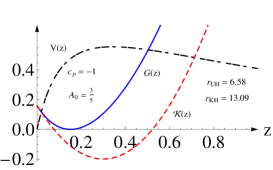
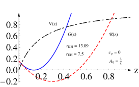
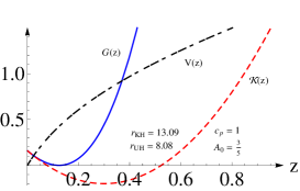
Figure 3: The functions $G,V\left(\equiv u^{r}\right)$ and ${\cal{K}}$ vs $z\equiv 1/r$ and the locations of the Killing ($r=r_{KH}$) and universal ($r=r_{UH}$) horizons, for the spacetime given by Eq.(IV.1.1) with $A_{0}=3/5$ and various choices of $c_{p}$.

When $\Lambda\not=0$, the mathematics becomes more involved. In the following we shall consider some representative choices of the parameter $\beta$.

Case 1.a $\beta=-1$: In the case, to have $D(r)\not=0$ for $r\in(0,\infty)$, we assume that $\frac{\bar{A}_{0}}{\Lambda-H^{2}}\leq 0$. In Fig. 4, we show the functions $G,V$ and ${\cal{K}}$ and the locations of the Killing and universal horizons for various choices of $c_{p}$.

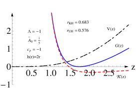
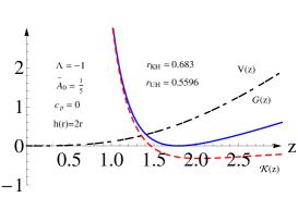
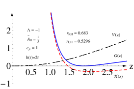
Figure 4: The functions $G,V\left(\equiv u^{r}\right)$ and ${\cal{K}}$ vs $z$, for the spacetime given by Eq.(4.33) with $\Lambda=-1,A_{0}=3/5,H=2,\beta=-1$ and various choices of $c_{p}$.

Case 1.b $\beta<-1$: In the case, to have $D(r)\not=0$ for $r\in(0,\infty)$, we must assume that either $\bar{A}_{0}\geq 0$ and $\Lambda<0$, or $\bar{A}_{0}\geq 0$, $\Lambda>0$. Then, in Fig. 5 we show the functions $G,V$ and ${\cal{K}}$ and the locations of the Killing and universal horizons for various choices of $c_{p}$ with $\beta=-2$.

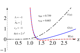
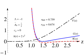
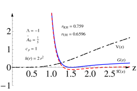
Figure 5: The functions $G,V\left(\equiv u^{r}\right)$ and ${\cal{K}}$ vs $z$, for the spacetime given by Eq.(4.33) with $\Lambda=-1,A_{0}=3/5,H=2,\beta=-2$ and various choices of $c_{p}$.

Case 1.c $0>\beta>-1$: In this case, we find that we must assume that either $\bar{A}_{0}>0,\;\Lambda<0$, or $\bar{A}_{0}>0,\;\Lambda>0$, in order not to have spacetime singularities at a finite and non-zero $r$. In Fig. 6, we show the functions $G,V$ and ${\cal{K}}$ and the locations of the Killing and universal horizons for various choices of $c_{p}$ with $\beta=-1/2$.

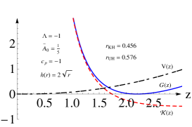
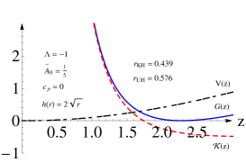
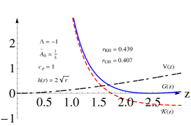
Figure 6: The functions $G,V\left(\equiv u^{r}\right)$ and ${\cal{K}}$ vs $z$, for the spacetime given by Eq.(4.33) with $\Lambda=-1,A_{0}=3/5,H=2,\beta=-1/2$ and various choices of $c_{p}$.

Case 1.d $\beta=0$: In the case, we must assume that $\frac{2\bar{A}_{0}+H^{2}}{\Lambda}\leq 0$, and in Fig. 7 we show the functions $G,V$ and ${\cal{K}}$ and the locations of the Killing and universal horizons.

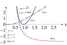
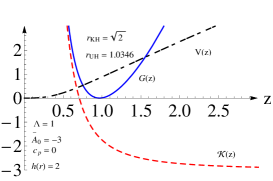
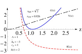
Figure 7: The functions $G,V\left(\equiv u^{r}\right)$ and ${\cal{K}}$ vs $z$, for the spacetime given by Eq.(4.33) with $\Lambda=-1,A_{0}=3/5,H=2,\beta=0$ and various choices of $c_{p}$.

Case 1.e $\beta>0$: In this case, we require that $\Lambda<0$. Then, in Fig. 8 we show the functions $G,V$ and ${\cal{K}}$ and the locations of the Killing and universal horizons for $\beta=2$.

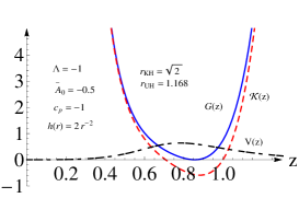
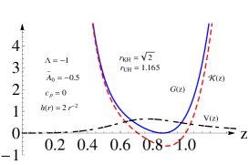
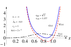
Figure 8: The functions $G,V\left(\equiv u^{r}\right)$ and ${\cal{K}}$ vs $z$, for the spacetime given by Eq.(4.33) with $\Lambda=-1,A_{0}=3/5,H=2,\beta=2$ and various choices of $c_{p}$.

IV.1.2 $\Lambda_{g}=0,\;\lambda\not=1$

In this case, the solutions are given by Eqs.(3.10), (3.14) and (3.15). Similar to the last case, without loss of the generality, we can always set $C_{1}=1$, and the metric takes the form,

$$ds^{2} = -\left(A_{0}+\frac{C_{3}^{2}}{2r^{2}}-\Lambda r^{2}\right)^{2}dt^{2}$$ (4.39)

$$+\left[dr+\left(C_{2}r+\frac{C_{3}}{r}\right)dt\right]^{2}+r^{2}d\theta^{2}.$$

To study these solutions further, let us consider the cases $C_{3}=0$ and $C_{3}\not=0$, separately.

When $C_{3}=0$, we assume that $C_{2}\not=0$. Otherwise, the metric will be singular across the Killing horizons. Then, the rescaling,

$$t\rightarrow C_{2}^{-1}t,~{}~{}A_{0}\rightarrow C_{2}A_{0},~{}~{}\Lambda\rightarrow C_{2}\Lambda,$$ (4.40)

leads the metric to the form,

$$ds^{2} = -\left(A_{0}-\Lambda r^{2}\right)^{2}dt^{2}+\left(dr+rdt\right)^{2}$$ (4.41)

$$+r^{2}d\theta^{2},\left(C_{3}=0\right),$$

from which we find that

$$R = 2\frac{A_{0}(3-8\Lambda^{2}r^{2})+4A_{0}^{2}\Lambda+\Lambda r^{2}+4\Lambda^{3}r^{4}}{(A_{0}-\Lambda r^{2})^{3}},$$

$$K = \frac{2}{A_{0}-\Lambda r^{2}}.$$ (4.42)

Thus, to avoid spacetime singularity at $A_{0}-\Lambda r^{2}=0$, we shall assume $A_{0}\Lambda\leq 0$. On the other hand, the Killing horizon is located at,

$$(A_{0}-\Lambda r_{KH}^{2})^{2}-r_{KH}^{2}=0,$$ (4.43)

which has real and positive roots only when $1+4A_{0}\Lambda\geq 0$. Moreover, in the present case Eq.(IV.1) reduces to

$$V^{\prime\prime}+\frac{A_{0}-3\Lambda r^{2}}{A_{0}r-\Lambda r^{3}}V^{\prime}$$

$$-\frac{A_{0}^{2}+2A_{0}c_{p}\Lambda r^{2}+(3-2c_{p})\Lambda^{2}r^{4}}{\left(A_{0}r-\Lambda r^{3}\right)^{2}}V=0.$$ (4.44)

In Fig. 9, we show the functions $G,V$ and ${\cal{K}}$ and the locations of the Killing and universal horizons for various choices of the free parameters, as specified in each of the panels of the figure.

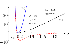
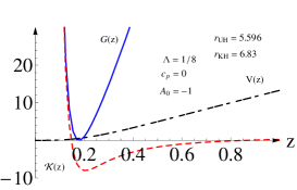
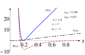
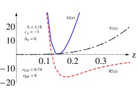
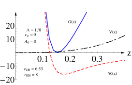
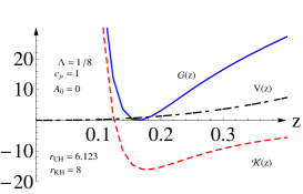
Figure 9: The functions $G,V$ and ${\cal{K}}$ and the locations of the Killing and universal horizons for the solutions given by Eq.(4.41) with $C_{3}=0$ for various choices of the free parameters.

When $C_{3}\not=0$, the rescaling of the timelike coordinate and the redefinitions of the parameters,

$$t\rightarrow C_{3}^{-1}t,~{}~{}A_{0}\rightarrow C_{3}A_{0},~{}~{}\Lambda\rightarrow C_{3}\Lambda,$$

$$C_{1}\rightarrow 2C_{A}/C_{3},$$ (4.45)

lead the metric to the form,

$$ds^{2} = -\left(A_{0}+\frac{C_{A}}{r^{2}}-\Lambda r^{2}\right)^{2}dt^{2}$$ (4.46)

$$+\left[dr+\left(C_{2}r+\frac{1}{r}\right)dt\right]^{2}+r^{2}d\theta^{2}.$$

If $C_{2}=0=\Lambda$, this metric becomes asymptotically flat at spatial infinity, and Eq.(IV.1) is given by

$$\frac{C_{A}^{2}(1-2c_{p})-2A_{0}C_{A}(c_{p}-2)r^{2}-A_{0}^{2}r^{4}}{r^{2}(A_{0}r^{2}+C_{A})^{2}}V$$

$$+V^{\prime\prime}+\frac{A_{0}r^{2}-C_{A}}{A_{0}r^{3}+C_{A}r}V^{\prime}=0.$$ (4.47)

In Fig. 10, we show the locations of the Killing and universal horizons.

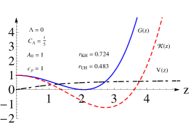
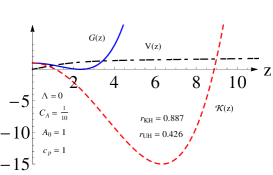
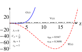
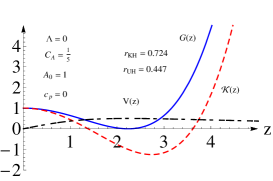
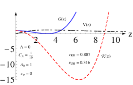
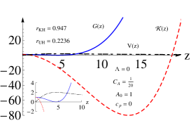
Figure 10: The functions $G,V$ and ${\cal{K}}$ and the locations of the Killing and universal horizons for the solutions given by Eq.(4.46) with $C_{c}=0=\Lambda$.

If $C_{2}$ and $\Lambda$ do not vanish at the same time, we find

$$R = \frac{2}{r^{2}{\cal{D}}(r)^{3}}\left[C_{A}^{2}(12\Lambda r^{4}-8A_{0}r^{2})\right.$$

$$-4C_{A}^{2}+C_{A}[r^{2}-4(A_{0}^{2}-C_{2})r^{4}-12\Lambda^{2}r^{8}$$

$$+(7C_{2}^{2}+16A_{0}\Lambda)r^{6}]+r^{4}[4A_{0}^{2}\Lambda r^{4}$$

$$+A_{0}(1+3C_{2}^{2}r^{4}-8\Lambda^{2}r^{6})+\Lambda r^{2}(4\Lambda^{2}r^{6}+C_{2}^{2}r^{4}$$

$$\left.+4C_{2}r^{2}-1)]\right],$$

$$K = \frac{2C_{2}r^{2}}{{\cal{D}}(r)},\;\;\;{\cal{D}}(r)\equiv C_{A}+A_{0}r^{2}-\Lambda r^{4}.$$ (4.48)

Again, to avoid spacetime singularities at finite but non-zero $r$, we must assume that ${\cal{D}}(r)\not=0$ for $r\in(0,\infty]$. In Fig. 11, we show the functions $G,V$ and ${\cal{K}}$ and the locations of the Killing and universal horizons.

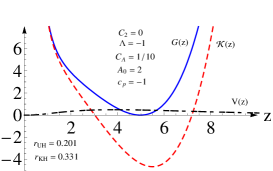
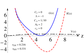
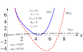
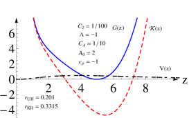
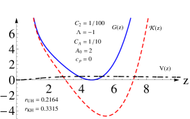
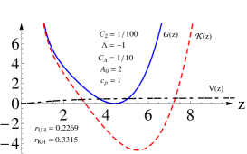
Figure 11: The functions $G,V$ and ${\cal{K}}$ and the locations of the Killing and universal horizons for the spacetimes given by Eq.(IV.1.2) with $C_{3}\not=0,\Lambda=-1,C_{2}=0$.

IV.1.3 $\Lambda_{g}\not=0$

When $\Lambda_{g}\not=0$, the solutions are mathematically much involved, and in this subsection we only consider the case where $\lambda\not=1$ but $C_{1}=0$. Then, the solutions are given by Eqs.(3.8), (3.22)-(III.1.2), for which the extrinsic curvature is given by

$$K = \frac{r^{\frac{\zeta-\lambda_{p}}{2\zeta}}}{2\zeta}\left[C_{-}r^{\frac{\lambda-5}{\lambda_{p}}}\left(\lambda_{p}-\zeta\right)-C_{+}\left(\lambda_{p}+\zeta\right)\right]$$ (4.49)

$$\times\left[\Lambda_{2}-A_{0}r-C_{+}^{2}\frac{r^{\frac{5-\lambda}{\lambda_{p}}-1}}{4\Lambda_{g}(1+3\lambda)}\left(\zeta(13+3\lambda_{p}\right.\right.$$

$$\left.-3\lambda)+8\right)-C_{-}^{2}\frac{r^{\frac{-5+\lambda}{\lambda_{p}}-1}}{4\Lambda_{g}(1+3\lambda)}\left(\zeta(-13+3\lambda_{p}\right.$$

$$\left.\left.+3\lambda)-8\right)\right]^{-1},$$

where $\lambda_{p}=\sqrt{(\lambda-1)(\lambda-5)}$ and $\zeta=\lambda-1$. Note that to have the metric real, as noticed in the last section, we must have either $\lambda\leq 1$ or $\lambda\geq 5$. When $\lambda\leq 1$, $\lambda$ should be larger than $-\frac{1}{3}$ so that $K$ remains finite at the spatial infinity.

In particular, for $\Lambda_{g}<0,\;\lambda=\frac{1}{2}$ and $C_{+}=0$, we have

$${\cal{N}}(r) = \Lambda_{2}-A_{0}r-\frac{9C_{2}^{2}}{20\Lambda_{g}r^{4}},$$

$$h(r) = \frac{C_{2}}{r},~{}~{}f(r)=-{\Lambda_{g}r^{2}},$$ (4.50)

where we had replaced $C_{-}$ by $C_{2}$. Then, Eq.(IV.1) can be rewritten as

$$\frac{V^{\prime\prime}}{V}+4\frac{5A_{0}\Lambda_{g}r^{5}-9C_{2}^{2}}{9C_{2}^{2}r+20r^{5}(A_{0}r-\Lambda_{2})\Lambda_{g}}\frac{V^{\prime}}{V}$$

$$-\left[9C_{2}^{2}r+20r^{5}(A_{0}r-\Lambda_{2})\Lambda_{g}\right]^{-2}\left[81C_{2}^{4}(5c_{p}-4)\right.$$

$$+180C_{2}^{2}r^{4}\Lambda_{g}\left(A_{0}(5c_{p}-28)r+20\Lambda_{2}-6c_{p}\Lambda_{2}\right)$$

$$\left.+400r^{8}\Lambda_{g}^{2}\left(A_{0}^{2}r^{2}-A_{0}c_{p}\Lambda_{2}r+c_{p}\Lambda_{2}^{2}\right)\right].$$ (4.51)

In Fig. 12, we show the functions ${\cal{K}}$, $V$ and $G$, and numerically find the radii of the Killing and universal horizons for $\lambda\leq 1$.

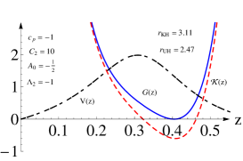
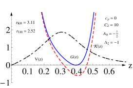
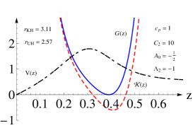
Figure 12: The functions $G,V$ and ${\cal{K}}$ and the locations of the Killing and universal horizons for the spacetimes given by Eq.(IV.1.3) with $\lambda\leq 1,\;\Lambda=-1$.

A similar consideration is presented in Fig. 13 for $\lambda\geq 5$. In particular, in this figure we have chosen $\lambda=\frac{19}{3}$, $\Lambda_{2}=1$, $\Lambda_{g}=-1$, $A_{0}=-2$, $C_{-}=2$ and $C_{+}=1$.

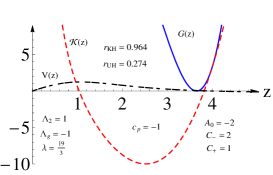
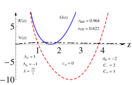
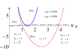
Figure 13: The functions $G,V$ and ${\cal{K}}$ and the locations of the Killing and universal horizons for the spacetimes given by Eq.(IV.1.3) with $\lambda=19/3>5,\;\Lambda=-1$.

In all the cases considered above, a universal horizon always exists inside a Killing horizon. To assure that no coordinate singularities appear across the Killing horizons, we are forced to use the PG-like coordinates, in which $N^{i}$ does not vanishes identically. Although not all of the solutions of the theory can be written in this form, as we mentioned above, the solutions considered in this paper indeed all possess these properties.

It is also important to note that the solutions presented above are the solutions of the full theory, that is, including the contribution of the higher-order derivative term specified by the coefficient $g_{2}$. Therefore, our above results show that universal horizons and black holes exist not only in the infrared limit, but also in the ultraviolet limit.

IV.2 Universal Horizons and Black Holes in Rotating Spacetimes

When spacetimes have rotations, the Killing horizons are different from the event horizons. The former are often called ergosurfaces (or ergospheres when the topology is $S^{n}$, where $n$ denotes the dimensions of the horizon), while the latter is defined by the existence of a null surface of the normal vector, $r_{\mu}\equiv\partial_{\mu}r$ Visser07 , that is,

$$\left.\gamma^{\mu\nu}r_{\mu}r_{\nu}\right|_{r=r_{e}}=\gamma^{rr}\left(r_{e}\right)=0.$$ (4.52)

In the following, we shall continuously denote the locations of the Killing horizons (or ergosurfaces) by $r_{KH}$, while the locations of the event horizons by $r_{e}$.

In the rotating spacetimes described by Eqs.(III.2), (III.2), (III.2) and (III.2), it is reasonable to assume that the khronon field $\phi$ depends only on $t$ and $r$, as all the metric coefficients are independent of $\theta$. Then, we find that $u_{\mu}\left(\propto\phi_{,\mu}\right)$ must take the form $u_{\mu}=\left(u_{t}(r),u_{r}(r),0\right)$, where $u_{t}=u_{t}\left(u_{r}\right)$, as now we have $\gamma^{\mu\nu}u_{\mu}u_{\nu}=-1$. Note that all of the three components $u^{\mu}=\left(u^{t},u^{r},u^{\theta}\right)$ in general do not vanish, due to the rotation, although both of $u^{t}$ and $u^{\theta}$ are not independent, and can be expressed as functions of $u_{r}$ (or equivalently as functions of $u^{r}$). With these in mind, we find that $V\left(\equiv u^{r}\right)$ satisfies the following differential equation,

$$\frac{V^{\prime\prime}}{V}+\left(\frac{{\cal{N}}^{\prime}}{{\cal{N}}}+\frac{1}{r}\right)\frac{V^{\prime}}{V}+\frac{{\cal{N}}^{\prime\prime}}{{\cal{N}}}$$

$$-\left(\frac{{\cal{N}}^{\prime}}{{\cal{N}}}\right)^{2}-\frac{1}{r^{2}}+\frac{c_{p}}{r}\frac{{\cal{N}}^{\prime}}{{\cal{N}}}=0,$$ (4.53)

which just depends on the function ${\cal{N}}$. To proceed further, we consider the three classes of solutions, separately.

IV.2.1 $R_{ij}=0,\;\lambda=1$

In this case, the rescaling

$$r\rightarrow C_{1}^{1/2}r,~{}~{}~{}\theta\rightarrow C_{1}^{-1/2}\theta,~{}~{}~{}h_{r}\rightarrow C_{1}^{1/2}h_{r},$$

$$h_{a}\rightarrow C_{1}^{1/2}h_{a},~{}~{}~{}h_{b}\rightarrow C_{1}^{-1/2}h_{b},$$ (4.54)

brings the metric into the form,

$$ds^{2} = -\left(A_{0}+\frac{H_{R}^{2}-\Lambda r^{2}}{2}\right)^{2}dt^{2}$$ (4.55)

$$+\left[dr\pm\sqrt{H_{R}^{2}-\frac{h_{a}^{2}}{r^{2}}}dt\right]^{2}$$

$$+r^{2}\left[d\theta+\left(\frac{h_{a}}{r^{2}}+h_{b}\right)dt\right]^{2},$$

where $H_{R}^{2}\equiv h_{r}(r)^{2}+\frac{h_{a}^{2}}{r^{2}}$. Recall that $h(r)$ is an arbitrary function of $r$, and $h_{a}$ and $h_{b}$ are the integration constants. Then, the killing horizon satisfies the equation,

$$\left(2A_{0}+{H_{R}^{2}-\Lambda r^{2}}\right)^{2}-4\left(H_{R}^{2}+2h_{a}h_{b}+h_{b}^{2}r^{2}\right)=0.$$

Choosing $H_{R}=\frac{h_{0}}{r^{\beta}}$ where $h_{0}$ is a constant, we have

$${\cal{N}}=A_{0}+\frac{h_{0}^{2}}{2r^{2\beta}}-\frac{\Lambda r^{2}}{2},$$ (4.57)

for which we find,

$$R = \frac{16h_{0}^{2}(1-\beta)r^{2\beta-2}}{D^{3}}\left[2A_{0}r^{2\beta}+h_{0}^{2}(1+\beta)\right]$$

$$+\frac{8}{R_{t}^{2}}\left[(h_{a}-1)h_{a}r^{2\beta}+h_{0}^{2}(2\beta^{2}+\beta-2)r^{2}\right]r^{2\beta-4}$$

$$+\frac{8}{r^{2}R_{t}}\left[2A_{0}r^{2\beta}+h_{0}^{2}(1-\beta^{2})\right]-\frac{8}{r^{2}},$$

$$K = \pm\frac{2h_{0}^{2}(1-\beta)}{\sqrt{h_{0}^{2}r^{2-2\beta}-h_{a}}D},$$ (4.58)

but now with $D(r)\equiv h_{0}^{2}+r^{2\beta}(\Lambda r^{2}-2A_{0})$. Again, to avoid spacetime singularities occurring at a finite and non-zero radius, we shall choose the free parameters so that $D(r)\not=0$ for $r\in(0,\infty]$. In Figs. 14 - 19, we show the functions $V,G,{\cal{K}}$ and the locations of the Killing and universal horizons for various choices of the free parameters, as indicated in each of the panels of the figures. From these figures one can see that universal horizons always exist.

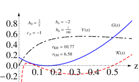
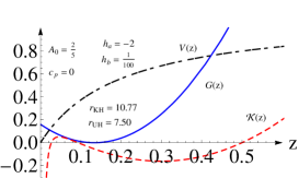
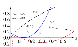
Figure 14: The functions $V,G,{\cal{K}}$ and the locations of the Killing, event and universal horizons in the case $\lambda=1$ of the rotating spacetimes given by Eq.(4.55) with $\Lambda=0$.

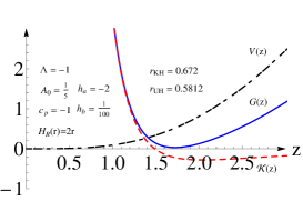
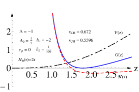
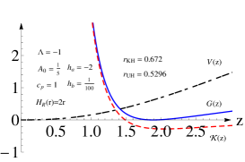
Figure 15: The functions $V,G,{\cal{K}}$ and the locations of the Killing, event and universal horizons in the case $\lambda=1$ of the rotating spacetimes given by Eq.(4.55) with $\Lambda\not=0$ and $\beta=-1$.

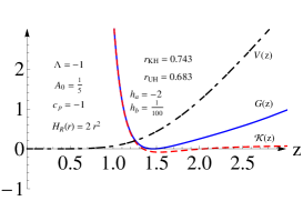
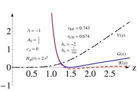
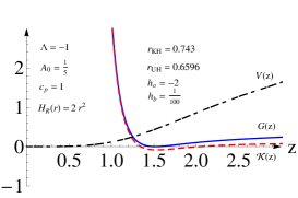
Figure 16: The functions $V,G,{\cal{K}}$ and the locations of the Killing, event and universal horizons in the case $\lambda=1$ of the rotating spacetimes given by Eq.(4.55) with $\Lambda\not=0$ and $\beta<-1$.

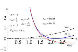
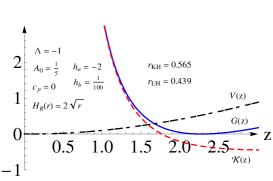
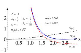
Figure 17: The functions $V,G,{\cal{K}}$ and the locations of the Killing, event and universal horizons in the case $\lambda=1$ of the rotating spacetimes given by Eq.(4.55) with $\Lambda\not=0$ and $\beta>-1$.

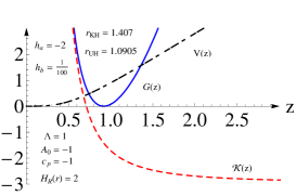
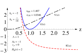
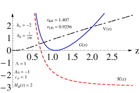
Figure 18: The functions $V,G,{\cal{K}}$ and the locations of the Killing, event and universal horizons in the case $\lambda=1$ of the rotating spacetimes given by Eq.(4.55) with $\Lambda\not=0$ and $\beta=0$.

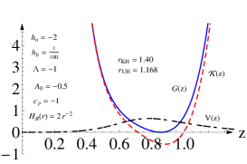
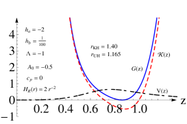
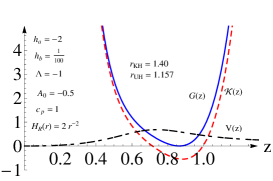
Figure 19: The functions $V$, $G$, $\cal K$ and the locations of the Killing, event and universal horizons in the case $\lambda=1$ of the rotating spacetimes given by Eq.(4.51) with $\Lambda\not=0$ and $\beta>0$.

IV.2.2 $R_{ij}=0,\;\lambda\not=1$

In this case, the solutions are given by Eq.(III.2), and the rescaling,

$$r\rightarrow C_{1}^{1/2}r,~{}~{}~{}\theta\rightarrow C_{1}^{-1/2}\theta,~{}~{}~{}h_{a}\rightarrow C_{1}^{1/2}h_{a},$$

$$h_{b}\rightarrow C_{1}^{-1/2}h_{b},~{}~{}~{}H_{A}\rightarrow C_{1}H_{A},$$ (4.59)

leads the metric to the form,

$$ds^{2} = -\left(A_{0}+\frac{H_{A}^{2}+h_{a}^{2}}{2r^{2}}-\frac{\Lambda_{C}}{2}r^{2}\right)^{2}dt^{2}$$ (4.60)

$$+\left[dr+\left(\frac{H_{A}}{r}+H_{B}r\right)dt\right]^{2}$$

$$+r^{2}\left[d\theta+\left(\frac{h_{a}}{r^{2}}+h_{b}\right)dt\right]^{2}.$$

The corresponding scalar and extrinsic curvatures are given by

$$R = -\frac{8}{r^{2}}+64R_{C}^{3}H_{B}r^{2}(H_{A}+H_{B}r^{2})(h_{a}^{2}+H_{A}^{2}+A_{0}r^{2})$$

$$+8R_{C}^{2}(h_{a}^{2}+H_{A}^{2}-4H_{A}H_{B}r^{2}-H_{B}^{2}r^{4})+16A_{0}R_{C},$$

$$K = 4H_{B}R_{C}r^{2},$$ (4.61)

where $R_{C}\equiv(h_{a}^{2}+H_{A}^{2}+2A_{0}r^{2}-\Lambda_{0}r^{4})^{-1}$ and $\Lambda_{0}\equiv\Lambda+H_{B}^{2}(1-2\lambda)$.

When $\Lambda_{C}\not=0$, we can simplify the above metric further by,

$$t\rightarrow-\frac{2}{\Lambda_{C}}t,~{}~{}~{}A_{0}\rightarrow-\frac{2}{\Lambda_{C}}A_{0},~{}~{}~{}H_{A}\rightarrow-\frac{2}{\Lambda_{C}}H_{A},$$

$$H_{B}\rightarrow-\frac{2}{\Lambda_{C}}H_{B},~{}h_{a}\rightarrow-\frac{2}{\Lambda_{C}}h_{a},~{}h_{b}\rightarrow-\frac{2}{\Lambda_{C}}h_{b},~{}~{}~{}~{}~{}~{}~{}$$ (4.62)

which leads Eq.(4.60) to,

$$ds^{2} = -\left(1+\frac{C_{A}}{r^{2}}+r^{2}\right)^{2}dt^{2}$$ (4.63)

$$+\left[dr+\left(\frac{H_{A}}{r}+H_{B}r\right)dt\right]^{2}$$

$$+r^{2}\left[d\theta+\left(\frac{h_{a}}{r^{2}}+h_{b}\right)dt\right]^{2},$$

where $C_{A}=-\frac{\Lambda_{C}}{4}\left(H_{A}^{2}+h_{a}^{2}\right)$. In Fig. 21 we show the locations of the Killing, event and universal horizons in this case.

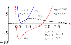
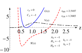
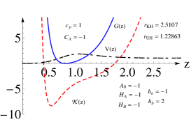
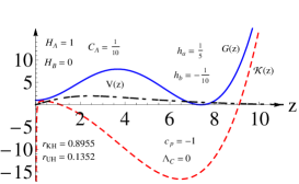
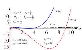
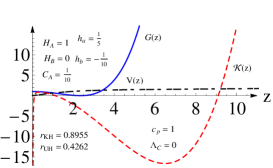
Figure 20: The functions $V,G,{\cal{K}}$ and the locations of the Killing, event and universal horizons in the case $\lambda\not=1$ of the rotating spacetimes given by Eq.(4.63) for $\Lambda_{C}\not=0$.

Figure 21: The functions $V,G,{\cal{K}}$ and the locations of the Killing, event and universal horizons in the case $\lambda=1$ of the rotating spacetimes given by Eq.(4.65) with $\Lambda_{C}=0$ but $A_{0}\not=0$.

When $\Lambda_{C}=0$, we assume $H_{B}\not=0$. Then, we consider the cases $A_{0}\not=0$ and $A_{0}=0$, separately. In particular, when $A_{0}\not=0$, the rescaling

$$t\rightarrow A_{0}^{-1}t,~{}~{}~{}H_{A}\rightarrow A_{0}H_{A},$$

$$h_{b}\rightarrow A_{0}h_{b},~{}~{}~{}h_{a}\rightarrow A_{0}h_{a},$$ (4.64)

leads to,

$$ds^{2} = -\left(1+\frac{C_{A}}{r^{2}}\right)^{2}dt^{2}+\left(dr+\frac{H_{A}}{r}dt\right)^{2}$$ (4.65)

$$+r^{2}\left[d\theta+\left(\frac{h_{a}}{r^{2}}+h_{b}\right)dt\right]^{2},$$

where $C_{A}=-\frac{A_{0}}{2}\left(H_{A}^{2}+h_{a}^{2}\right)$. Fig. 21 shows the locations of the Killing and universal horizons.

When $A_{0}=0$, the rescaling,

$$t\rightarrow C_{H}t,~{}~{}~{}H_{A}\rightarrow C_{H}^{-1}H_{A},$$

$$h_{b}\rightarrow C_{H}^{-1}h_{b},~{}~{}~{}h_{a}\rightarrow C_{H}^{-1}h_{a},$$ (4.66)

leads to,

$$ds^{2} = -\frac{dt^{2}}{r^{4}}+\left[dr+\frac{H_{A}}{r}dt\right]^{2}$$ (4.67)

$$+r^{2}\left[d\theta+\left(\frac{h_{a}}{r^{2}}+h_{b}\right)dt\right]^{2},$$

where $C_{H}=\frac{2}{H_{A}^{2}+h_{a}^{2}}$. In this case, the equation of $V$ takes the simple form,

$$V^{\prime\prime}-\frac{V^{\prime}}{r}+(1-2c_{p})\frac{V}{r^{2}}=0,$$ (4.68)

and has the solution,

$$V=r_{A}r^{1+\sqrt{2c_{p}}}+r_{B}r^{1-\sqrt{2c_{p}}}.$$ (4.69)

Consider the boundary condition $V(\infty)\rightarrow 0$, we have $r_{A}=0$, so $G$ is given by

$$G=\frac{1+r_{B}^{2}r^{2-2\sqrt{2c_{p}}}}{r^{4}}-\frac{H_{A}^{2}}{r^{2}}.$$ (4.70)

Clearly, $G<0$ as $r\rightarrow\infty$, which is not allowed by the existence of the khronon field in the whole spacetime. Therefore, in this case the solution must be discarded.

IV.2.3 $R_{ij}\not=0$

In this case, the solutions are given by Eqs.(III.2) and (III.2), and the corresponding spacetimes with $a_{i}=(1,0)$ describes a spacetime, but the metric at the killing horizon located at $f(r_{KH})=0$ becomes singular. Therefore, to study the location of the universal horizon inside it, an extension of the solution into the internal of the Killing horizon is needed. Such extension is standard Sotiriou:2014gna , so in the following we shall not consider it further.

V Conclusions

In this paper, we have studied the existence of universal horizons and black holes in gravitational theories with broken Lorentz invariance. We have paid particular attention to the case where the gravitational field is so strong that the infrared limit does not exist, and the higher-order derivative terms must be included, in order for the theory to be UV complete. We have shown that even in the UV regime both static and rotating universal horizons and black holes exist. Therefore, universal horizons and black holes are not only the low energy phenomena but also phenomena existing in the UV regime. To reach this conclusion, we have first constructed exact solutions of the full theory of Hořava gravity with the projectability and U(1) symmetry in (2+1)-dimensions, which is power-counting renormalizable HMT ; WW ; Silva ; HW . To avoid coordinate singularities across the Killing horizons, we have chosen to work with the PG-like coordinates PG . Although this normally makes the field equations very complicated, we are still able to find analytical solutions in both static and stationary spacetimes. Then, we have numerically solved the khronon field equations, and identified the locations of the universal horizons. In all the cases considered, universal horizons exist, and are always located inside the Killing horizons.

With these exact solutions, we hope that the study of black hole thermodynamics at the universal horizons, specially the ones with rotations, can be made more accessible. In the spherically symmetric and neutral case, the first law of black hole thermodynamics at universal horizons holds Berglund:2012bu , provided that the entropy is still proportional to the area of the horizon, and the surface gravity is defined by,

$$\kappa\equiv\frac{1}{2}u^{\alpha}D_{\alpha}\left(u_{\lambda}\zeta^{\lambda}\right),$$ (5.1)

which is identical to the one obtained from the peeling behavior of the khronon field Cropp:2013sea , as shown explicitly in Lin:2014eaa . In the neutral case, the temperature of the black hole takes its standard form, $T=\kappa/2\pi$ Berglund:2012fk ; Cropp:2013sea . However, when the black hole is charged, such a first law does not exist Ding:2015kba , if we insist that the temperature of the black hole still takes its standard form with the surface gravity given as above, and that the entropy of the black hole is proportional to its area. In addition, when high-order powers of momentum appear in the dispersion relation of the particles emitted through the Hawking radiation process, which generically is always the case, the temperature of the black hole at the universal horizon depends on the order of the powers, although it is still proportional to the surface gravity $\kappa$ defined above JB13 ; Ding:2015fyx .

We also hope that these exact solutions will help us to get deeper insights into the problem of quantization of the theory Carlip ; Kiefer , and the non-relativistic AdS/CFT correspondence Kachru:2008yh ; LSWW ; Janiszewski:2014ewa ; Basu:2016vyz . The studies of these important issues are out of scope of this paper, and we wish to come back to them in a different occasion.

Finally, we would like to note that our main conclusion regarding the existence of universal horizons and black holes at all energy scales (including the UV regime) should be easily generalized to other versions of Hořava gravity Horava:2011gd ; Wang:2012nv , although in this paper we have considered it only in the projectable Hořava theory with an extra U(1) symmetry HMT ; WW ; Silva ; HW . It is also quite reasonable to expect that this is also the generic case in other theories of gravity without Lorentz symmetry.

Appendix A. Projectable Hořava theory with U(1) symmetry in (d+1) dimensions

In this Appendix, we give a brief introduction to the projectable Hořava theory with U(1) symmetry. for detail, we refer readers to HMT ; WW ; Silva ; HW .

V.1 The Gauge Symmetries

The Hořava theory is based on the perspective that Lorentz symmetry should appear as an emergent symmetry at long distances, but can be fundamentally absent at short ones Pav . In the latter regime, the system exhibits a strong anisotropic scaling between space and time,

$${\bf x}\rightarrow\ell{\bf x},\;\;\;t\rightarrow\ell^{z}t,$$ (A.1)

where $z\geq 3$ in the $(3+1)$-dimensional spacetime Horava ; Visser . At long distances, higher-order curvature corrections become negligible, and the lowest order terms $R$ and $\Lambda$ take over, whereby the Lorentz invariance is expected to be “accidentally restored,” where $R$ denotes the 3-dimensional Ricci scalar, and $\Lambda$ the cosmological constant. Because of the anisotropic scaling, the gauge symmetry of the theory is broken down to the foliation-preserving diffeomorphism, Diff($M,\;{\cal{F}}$),

$$\tilde{t}=t-f(t),\;\;\;\tilde{x}^{i}={x}^{i}-\zeta^{i}(t,{\bf x}),$$ (A.2)

for which the lapse function $N$, shift vector $N^{i}$, and 3-spatial metric $g_{ij}$ transform as

$$\delta{N} = \zeta^{k}\nabla_{k}N+\dot{N}f+N\dot{f},$$

$$\delta{N}_{i} = N_{k}\nabla_{i}\zeta^{k}+\zeta^{k}\nabla_{k}N_{i}+g_{ik}\dot{\zeta}^{k}+\dot{N}_{i}f+N_{i}\dot{f},$$

$$\delta{g}_{ij} = \nabla_{i}\zeta_{j}+\nabla_{j}\zeta_{i}+f\dot{g}_{ij},$$ (A.3)

where $\dot{f}\equiv df/dt,\;\nabla_{i}$ denotes the covariant derivative with respect to $g_{ij}$, $N_{i}=g_{ik}N^{k}$, and $\delta{g}_{ij}\equiv{\gamma}_{ij}\left(t,x^{k}\right)-{g}_{ij}\left(t,x^{k}\right)$, etc. From these expressions one can see that $N$ and $N^{i}$ play the role of gauge fields of the Diff($M,\;{\cal{F}}$). Therefore, it is natural to assume that $N$ and $N^{i}$ inherit the same dependence on space and time as the corresponding generators Horava ,

$$N=N(t),\;\;\;N^{i}=N^{i}(t,x),$$ (A.4)

which is often referred to as the projectability condition.

Due to the Diff($M,\;{\cal{F}}$) diffeomorphisms (A.2), one more degree of freedom appears in the gravitational sector - a spin-0 graviton. This is potentially dangerous, and needs to decouple in the IR regime, in order to be consistent with observations. A very promising approach along this direction is to eliminate the spin-0 graviton by introducing two auxiliary fields, the $U(1)$ gauge field $A$ and the Newtonian prepotential $\varphi$, by extending the Diff($M,\;{\cal{F}}$) symmetry (A.2) to include a local $U(1)$ symmetry HMT ,

$$U(1)\ltimes{\mbox{Diff}}(M,\;{\cal{F}}).$$ (A.5)

Under this extended symmetry, the special status of time maintains, so that the anisotropic scaling (A.1) can still be realized, and the theory is UV complete. Meanwhile, because of the elimination of the spin-0 graviton, its IR behavior can be significantly improved. Under the Diff($M,\;{\cal{F}}$), $A$ and $\varphi$ transform as,

$$\delta{A} = \zeta^{i}\partial_{i}A+\dot{f}A+f\dot{A},$$

$$\delta\varphi = f\dot{\varphi}+\zeta^{i}\partial_{i}\varphi.$$ (A.6)

Under the local $U(1)$ symmetry, the fields transform as

$$\delta_{\alpha}A = \dot{\alpha}-N^{i}\nabla_{i}\alpha,\;\;\;\delta_{\alpha}\varphi=-\alpha,$$

$$\delta_{\alpha}N_{i} = N\nabla_{i}\alpha,\;\;\;\delta_{\alpha}g_{ij}=0,\;\;\;\delta_{\alpha}{N}=0,$$ (A.7)

where $\alpha$ is the generator of the local $U(1)$ gauge symmetry. For the detail, we refer readers to HMT ; WW .

The elimination of the spin-0 graviton was done initially in the case $\lambda=1$ HMT ; WW , but soon generalized to the case with any $\lambda$ Silva ; HW ; LWWZ , where $\lambda$ denotes a coupling constant that characterizes the deviation of the kinetic part of action from the corresponding one given in GR with $\lambda_{GR}=1$. For the analysis of Hamiltonian consistency, see HMT ; Kluson .

V.2 Universal Coupling with Matter and Field Equations

The basic variables in the HMT setup are

$$\left(A,\;\varphi,\;N,\;N^{i},\;g_{ij}\right),\;(i,j=1,2,...,d),$$ (A.8)

and the total action of the theory in ($d+1$)-diemnsions can be written in the form,

$$S = \zeta^{2}\int dtd^{d}xN\sqrt{g}\Big{(}{\cal{L}}_{K}-{\cal{L}}_{{V}}+{\cal{L}}_{{\varphi}}+{\cal{L}}_{{A}}+{\zeta^{-2}}{\cal{L}}_{M}\Big{)},$$

where $g={\rm det}(g_{ij})$, $\zeta^{2}={1}/{(16\pi G)}$, and

$${\cal{L}}_{K} = K_{ij}K^{ij}-\lambda K^{2},$$

$${\cal{L}}_{\varphi} = \varphi{\cal{G}}^{ij}\Big{(}2K_{ij}+\nabla_{i}\nabla_{j}\varphi\Big{)}$$

$$+\big{(}1-\lambda\big{)}\Big{[}\big{(}\Delta\varphi\big{)}^{2}+2K\Delta\varphi\Big{]},$$

$${\cal{L}}_{A} = \frac{A}{N}\Big{(}2\Lambda_{g}-R\Big{)}.$$ (A.10)

Here $\Delta\equiv g^{ij}\nabla_{i}\nabla_{j}$, $\Lambda_{g}$ is a coupling constant with dimension of $({\mbox{length}})^{-2}$, the Ricci and Riemann tensors $R_{ij}$ and $R^{i}_{jkl}$ all refer to the d-dimensional metric $g_{ij}$, and

$$K_{ij} = \frac{1}{2N}\left(-\dot{g}_{ij}+\nabla_{i}N_{j}+\nabla_{j}N_{i}\right),$$

$${\cal{G}}_{ij} = R_{ij}-\frac{1}{2}g_{ij}R+\Lambda_{g}g_{ij}.$$ (A.11)

${\cal{L}}_{{V}}$ is an arbitrary Diff($\Sigma$)-invariant local scalar functional built out of the spatial metric, its Riemann tensor and spatial covariant derivatives, without the use of time derivatives.

${\cal{L}}_{{M}}$ is the Lagrangian of matter fields, which is a scalar not only with respect to the ${\mbox{Diff}}(M,{\cal{F}})$ symmetry (A.2), but also to the $U(1)$ symmetry (V.1). When the gravity is universally coupled with matter, it is given by LMWZ

$$S_{M} = \int dtd^{d}xN\sqrt{g}{\cal{L}}_{M}\left(A,\;\varphi,\;N,\;N^{i},\;g_{ij};\psi_{n}\right)$$ (A.12)

$$= \int d^{d+1}x\sqrt{|\gamma|}\;\tilde{{\cal{L}}}_{M}\left(\gamma_{\mu\nu};\psi_{n}\right),$$

where $\gamma\equiv det(\gamma_{\mu\nu})\;(\mu,\nu=0,1,...,d)$, and $\psi_{n}$ collectively stands for matter fields, minimally coupled to the (d+1)-dimensional metric $\gamma_{\mu\nu}$, defined as

$$\left(\gamma_{\mu\nu}\right) \equiv \left(\matrix{-{\cal{N}}^{2}+{\cal{N}}^{i}{\cal{N}}_{i}&{\cal{N}}_{i}\cr{\cal{N}}_{i}&{\gamma}_{ij}\cr}\right),$$

$$\left(\gamma^{\mu\nu}\right) = \left(\matrix{-\frac{1}{{\cal{N}}^{2}}&\frac{{\cal{N}}^{i}}{{\cal{N}}^{2}}\cr\frac{{\cal{N}}^{i}}{{\cal{N}}^{2}}&{\gamma}^{ij}-\frac{{\cal{N}}^{i}{\cal{N}}^{j}}{{\cal{N}}^{2}}\cr}\right),$$ (A.13)

where ${\gamma}^{ij}{\gamma}_{ik}=\delta^{j}_{k},\;{\cal{N}}_{i}\equiv{\gamma}_{ij}{\cal{N}}^{j}$, and

$${\cal{N}}=\left(1-a_{1}\sigma\right)N,\;\;\;{\cal{N}}^{i}=N^{i}+Ng^{ij}\nabla_{j}\varphi,$$

$${\gamma}_{ij}=\left(1-a_{2}\sigma\right)^{2}g_{ij},\;\;\;\sigma=\frac{A-{\cal{A}}}{N},$$

$${\cal{A}}\equiv-\dot{\varphi}+N^{i}\nabla_{i}\varphi+\frac{1}{2}N\left(\nabla^{i}\varphi\right)\left(\nabla_{i}\varphi\right).$$ (A.14)

Here $a_{1}$ and $a_{2}$ are two arbitrary constants. It is should be noted that the line element

$$ds^{2} = \gamma_{\mu\nu}dx^{\mu}dx^{\nu}=-{\cal{N}}^{2}dt^{2}$$ (A.15)

$$+{\gamma}_{ij}\left(dx^{i}+{\cal{N}}^{i}dt\right)\left(dx^{j}+{\cal{N}}^{j}dt\right),~{}~{}~{}~{}$$

is invariant not only under the gauge transformations (A.2), but also under the U(1) transformations (V.1). In terms of $\tilde{{\cal{L}}}_{M}$, the (d+1)-dimensional energy-momentum tensor $T_{\mu\nu}$ is given by

$$T^{\mu\nu}\equiv\frac{1}{\sqrt{|\gamma|}}\frac{\delta\left(\sqrt{|\gamma|}{\tilde{\cal{L}}}_{M}(\gamma_{\alpha\beta};\psi_{n})\right)}{\delta\gamma_{\mu\nu}}.$$ (A.16)

The variations of the total action with respect to $N$ and $N^{i}$ yield the Hamiltonian and momentum constraints, given, respectively, by,

$$\int{d^{d}x\sqrt{g}\left[{\cal{L}}_{K}+{\cal{L}}_{{V}}-\varphi{\cal{G}}^{ij}\nabla_{i}\nabla_{j}\varphi-\big{(}1-\lambda\big{)}\big{(}\Delta\varphi\big{)}^{2}\right]}$$

$$~{}~{}~{}~{}~{}~{}~{}~{}~{}~{}~{}~{}~{}~{}~{}~{}~{}~{}~{}~{}~{}~{}~{}~{}~{}~{}~{}~{}~{}=8\pi G\int d^{d}x{\sqrt{g}\,J^{t}},$$ (A.17)

$$\nabla^{j}\Big{[}\pi_{ij}-\varphi{\cal{G}}_{ij}-\big{(}1-\lambda\big{)}g_{ij}\nabla^{2}\varphi\Big{]}=8\pi GJ_{i},$$ (A.18)

where

$$J^{t} \equiv 2\frac{\delta\left(N{\cal{L}}_{M}\right)}{\delta N},\;\;\;J_{i}\equiv-N\frac{\delta{\cal{L}}_{M}}{\delta N^{i}},$$

$$\pi^{ij} \equiv \frac{\delta(N{\cal{L}}_{K})}{\delta\dot{g}_{ij}}=-K^{ij}+\lambda Kg^{ij}.$$ (A.19)

Variation of the action (V.2) with respect to $\varphi$ and $A$ yield,

$${\cal{G}}^{ij}\Big{(}K_{ij}+\nabla_{i}\nabla_{j}\varphi\Big{)}+\big{(}1-\lambda\big{)}\Delta\Big{(}K+\Delta\varphi\Big{)}$$

$$~{}~{}~{}~{}~{}~{}~{}~{}~{}~{}~{}~{}~{}~{}~{}~{}~{}~{}~{}~{}~{}~{}~{}~{}~{}~{}~{}~{}~{}~{}~{}~{}=8\pi GJ_{\varphi},$$ (A.20)

$$R-2\Lambda_{g}=8\pi GJ_{A},$$ (A.21)

which will be referred, respectively, to as the $\varphi$- and $A$- constraint, where

$$J_{\varphi}\equiv-\frac{\delta{\cal{L}}_{M}}{\delta\varphi},\;\;\;J_{A}\equiv 2\frac{\delta\left(N{\cal{L}}_{M}\right)}{\delta{A}}.$$ (A.22)

On the other hand, the dynamical equations now read,

$$\frac{1}{N\sqrt{g}}\Bigg{\{}\sqrt{g}\Big{[}\pi^{ij}-\varphi{\cal{G}}^{ij}-\big{(}1-\lambda\big{)}g^{ij}\Delta\varphi\Big{]}\Bigg{\}}_{,t}$$ (A.23)

$$~{}~{}~{}=-2\left(K^{2}\right)^{ij}+2\lambda KK^{ij}-\frac{2}{N}\pi^{k(i}\nabla_{k}N^{j)}$$

$$~{}~{}~{}~{}~{}+\nabla_{k}\Big{[}\frac{N^{k}}{N}\pi^{ij}-(1-\lambda)F^{k}_{\varphi}g^{ij}\Big{]}$$

$$~{}~{}~{}~{}~{}-2\big{(}1-\lambda\big{)}\Big{[}\big{(}K+\Delta\varphi\big{)}\nabla^{i}\nabla^{j}\varphi+K^{ij}\Delta\varphi\Big{]}$$

$$~{}~{}~{}~{}~{}+2(1-\lambda)\nabla^{(i}\left[\nabla^{j)}\varphi\left(K+\Delta\varphi\right)\right]$$

$$~{}~{}~{}~{}~{}+\frac{1-\lambda}{N}\Delta\varphi\nabla^{(i}N^{j)}$$

$$~{}~{}~{}~{}~{}+\frac{1}{2}\Big{(}{\cal{L}}_{K}+{\cal{L}}_{\varphi}+{\cal{L}}_{A}\Big{)}g^{ij}$$

$$~{}~{}~{}~{}~{}+F^{ij}+F_{\varphi}^{ij}+F_{A}^{ij}+8\pi G{\cal{N}}^{ij},$$

where $\left(K^{2}\right)^{ij}\equiv K^{il}K_{l}^{j},\;f_{(ij)}\equiv\left(f_{ij}+f_{ji}\right)/2$, and

$$F^{ij} \equiv -\frac{1}{\sqrt{g}}\frac{\delta\left(\sqrt{g}{\cal{L}}_{V}\right)}{\delta{g}_{ij}},$$

$$F_{\varphi}^{ij} = \sum^{3}_{n=1}{F_{(\varphi,n)}^{ij}},$$

$$F_{\varphi}^{i} = \Big{(}K+\nabla^{2}\varphi\Big{)}\nabla^{i}\varphi+\frac{N^{i}}{N}\Delta\varphi,$$

$$F_{A}^{ij} = \frac{1}{N}\left[AR^{ij}-\Big{(}\nabla^{i}\nabla^{j}-g^{ij}\Delta\Big{)}A\right],$$

with $n_{{\scriptscriptstyle S}}=(2,0,-2,-2)$, and $F_{(\varphi,n)}^{ij}$ are given by WW ,

$$F_{(\varphi,1)}^{ij} = \frac{1}{2}\varphi\left\{\Big{(}2K+\nabla^{2}\varphi\Big{)}R^{ij}-2\Big{(}2K^{j}_{k}+\nabla^{j}\nabla_{k}\varphi\Big{)}R^{ik}\right.$$

$$~{}~{}~{}~{}~{}-2\Big{(}2K^{i}_{k}+\nabla^{i}\nabla_{k}\varphi\Big{)}R^{jk}$$

$$~{}~{}~{}~{}~{}\left.-\Big{(}2\Lambda_{g}-R\Big{)}\Big{(}2K^{ij}+\nabla^{i}\nabla^{j}\varphi\Big{)}\right\},$$

$$F_{(\varphi,2)}^{ij} = \frac{1}{2}\nabla_{k}\left\{\varphi{\cal{G}}^{ik}\Big{(}\frac{2N^{j}}{N}+\nabla^{j}\varphi\Big{)}\right.$$

$$\left.+\varphi{\cal{G}}^{jk}\Big{(}\frac{2N^{i}}{N}+\nabla^{i}\varphi\Big{)}-\varphi{\cal{G}}^{ij}\Big{(}\frac{2N^{k}}{N}+\nabla^{k}\varphi\Big{)}\right\},$$

$$F_{(\varphi,3)}^{ij} = \frac{1}{2}\left\{2\nabla_{k}\nabla^{(i}f^{j)k}_{\varphi}-\nabla^{2}f_{\varphi}^{ij}-\left(\nabla_{k}\nabla_{l}f^{kl}_{\varphi}\right)g^{ij}\right\},$$

where

$$f_{\varphi}^{ij} = \varphi\left\{\Big{(}2K^{ij}+\nabla^{i}\nabla^{j}\varphi\Big{)}-\frac{1}{2}\Big{(}2K+\nabla^{2}\varphi\Big{)}g^{ij}\right\}.$$

The tensor ${\cal{N}}^{ij}$ is defined as

$${\cal{N}}^{ij}={2\over\sqrt{g}}{\delta\left(\sqrt{g}{\cal{L}}_{M}\right)\over\delta{g}_{ij}}.$$ (A.27)

The conservation laws of energy and momentum of matter fields read, respectively,

$$\int d^{d}x\sqrt{g}{\left[\dot{g}_{kl}{\cal{N}}^{kl}-\frac{1}{\sqrt{g}}\left(\sqrt{g}J^{t}\right)_{,t}+\frac{2N_{k}}{N\sqrt{g}}\left(\sqrt{g}J^{k}\right)_{,t}\right.}$$

$$~{}~{}~{}~{}~{}~{}~{}~{}~{}~{}~{}~{}~{}~{}\left.-2\dot{\varphi}J_{\varphi}-\frac{A}{N\sqrt{g}}\left(\sqrt{g}J_{A}\right)_{,t}\right]=0,$$ (A.28)

$$\nabla^{k}{\cal{N}}_{ik}-\frac{1}{N\sqrt{g}}\left(\sqrt{g}J_{i}\right)_{,t}-\frac{J^{k}}{N}\left(\nabla_{k}N_{i}-\nabla_{i}N_{k}\right)$$

$$\;\;\;\;\;\;\;\;\;\;\;-\frac{N_{i}}{N}\nabla_{k}J^{k}+J_{\varphi}\nabla_{i}\varphi-\frac{J_{A}}{2N}\nabla_{i}A=0.$$ (A.29)

Introducing the normal vector $n_{\nu}$ to the hypersurface $t=$ constant,

$$n_{\mu}=-{\cal{N}}\delta^{t}_{\mu},\;\;\;n^{\mu}=\frac{1}{{\cal{N}}}\left(1,-{\cal{N}}^{i}\right),$$ (A.30)

one can decompose $T_{\mu\nu}$ as Anninos:2001yc ,

$$\rho_{H} \equiv T_{\mu\nu}n^{\mu}n^{\nu},$$

$$s_{i} \equiv -T_{\mu\nu}\left(\delta^{\mu}_{i}+n^{\mu}n_{i}\right)n^{\nu},$$

$$s_{ij} \equiv T_{\mu\nu}\left(\delta^{\mu}_{i}+n^{\mu}n_{i}\right)\left(\delta^{\nu}_{j}+n^{\nu}n_{j}\right),$$ (A.31)

in terms of which, the quantities $J^{t},\;J_{i},\;J_{A},\;J_{\varphi}$ and ${\cal{N}}_{ij}$ are given by LMWZ ,

$$J^{t} = 2\Omega^{3}(\sigma)\Bigg{\{}-\rho_{H}\frac{\delta{\cal{N}}}{\delta{N}}+\frac{\delta{\cal{N}}_{i}}{\delta{N}}s^{i}+\frac{1}{2}{\cal{N}}\frac{\delta{\gamma}_{ij}}{\delta{N}}s^{ij}\Bigg{\}},$$

$$J^{i} = -\Omega^{3}(\sigma)\Bigg{\{}-\rho_{H}\frac{\delta{\cal{N}}}{\delta{N}_{i}}+\frac{\delta{\cal{N}}_{k}}{\delta{N}_{i}}s^{k}+\frac{1}{2}{\cal{N}}\frac{\delta{\gamma}_{kl}}{\delta{N}_{i}}s^{kl}\Bigg{\}},$$

$${\cal{N}}^{ij} = \frac{2\Omega^{3}(\sigma)}{N}\Bigg{\{}-\rho_{H}\frac{\delta{\cal{N}}}{\delta{g}_{ij}}+\frac{\delta{\cal{N}}_{k}}{\delta{g}_{ij}}s^{k}+\frac{1}{2}{\cal{N}}\frac{\delta{\gamma}_{kl}}{\delta{g}_{ij}}s^{kl}\Bigg{\}},$$

$$J_{A} = 2\Omega^{3}(\sigma)\Bigg{\{}-\rho_{H}\frac{\delta{\cal{N}}}{\delta{A}}+\frac{\delta{\cal{N}}_{k}}{\delta{A}}s^{k}+\frac{1}{2}{\cal{N}}\frac{\delta{\gamma}_{kl}}{\delta{A}}s^{kl}\Bigg{\}},$$

$$J_{\varphi} = -\frac{1}{N}\Bigg{\{}\frac{1}{\sqrt{g}}\left(B\sqrt{g}\right)_{,t}-\nabla_{i}\Big{[}B\left(N^{i}+N\nabla^{i}\varphi\right)\Big{]}$$ (A.32)

$$~{}~{}~{}~{}~{}~{}~{}~{}~{}-\nabla_{i}\left(N\Omega^{5}s^{i}\right)\Bigg{\}},$$

where $\Omega\equiv 1-a_{2}\sigma$, and

$$B \equiv -\Omega^{3}(\sigma)\Bigg{\{}a_{1}\rho_{H}-\frac{2a_{2}\left(1-a_{2}\sigma\right)}{N}s^{k}\left(N_{k}+N\nabla_{k}\varphi\right)$$ (A.33)

$$-a_{2}\left(1-a_{1}\sigma\right)\left(1-a_{2}\sigma\right)g_{ij}s^{ij}\Bigg{\}},$$

and

$$\frac{\delta{\cal{N}}}{\delta{N}} = 1+\frac{1}{2}a_{1}\left(\nabla_{k}\varphi\right)^{2},$$

$$\frac{\delta{\cal{N}}_{i}}{\delta{N}} = \frac{\Omega}{N}\Bigg{\{}N\Omega\nabla_{i}\varphi$$

$$~{}~{}~{}~{}~{}~{}+2a_{2}\left(N_{i}+N\nabla_{i}\varphi\right)\left[\sigma+\frac{1}{2}\left(\nabla_{k}\varphi\right)^{2}\right]\Bigg{\}},$$

$$\frac{\delta{\gamma}_{ij}}{\delta{N}} = \frac{2a_{2}\Omega}{N}\left[\sigma+\frac{1}{2}\left(\nabla_{k}\varphi\right)^{2}\right]g_{ij},$$

$$\frac{\delta{\cal{N}}}{\delta{N}_{i}} = a_{1}\nabla^{i}\varphi,$$

$$\frac{\delta{\cal{N}}_{k}}{\delta{N}_{i}} = \frac{\Omega}{N}\Big{\{}N\Omega\delta^{i}_{k}+2a_{2}\left(N_{k}+N\nabla_{k}\varphi\right)\nabla^{i}\varphi\Big{\}},$$

$$\frac{\delta{\gamma}_{kl}}{\delta{N}_{i}} = \frac{2a_{2}\Omega}{N}g_{kl}\nabla^{i}\varphi,$$

$$\frac{\delta{\cal{N}}}{\delta{g}_{ij}} = -a_{1}\Bigg{[}N^{(i}\nabla^{j)}\varphi+\frac{1}{2}N\left(\nabla^{i}\varphi\right)\left(\nabla^{j}\varphi\right)\Bigg{]},$$

$$\frac{\delta{\cal{N}}_{k}}{\delta{g}_{ij}} = -\frac{2a_{2}\Omega}{N}\left(N_{k}+N\nabla_{k}\varphi\right)$$

$$\times\Bigg{[}N^{(i}\nabla^{j)}\varphi+\frac{1}{2}N\left(\nabla^{i}\varphi\right)\left(\nabla^{j}\varphi\right)\Bigg{]},$$

$$\frac{\delta{\gamma}_{kl}}{\delta{g}_{ij}} = \frac{1}{2}\Omega^{2}\left(\delta^{i}_{k}\delta^{j}_{l}+\delta^{i}_{l}\delta^{j}_{k}\right)$$

$$-\frac{2a_{2}\Omega g_{kl}}{N}\Bigg{[}N^{(i}\nabla^{j)}\varphi+\frac{1}{2}N\left(\nabla^{i}\varphi\right)\left(\nabla^{j}\varphi\right)\Bigg{]},$$

$$\frac{\delta{\cal{N}}}{\delta{A}} = -a_{1},$$

$$\frac{\delta{\cal{N}}_{i}}{\delta{A}} = -\frac{2a_{2}\Omega}{N}\left(N_{i}+N\nabla_{i}\varphi\right),$$

$$\frac{\delta{\gamma}_{ij}}{\delta{A}} = -\frac{2a_{2}\Omega}{N}g_{ij}.$$ (A.34)

For the gauge $\varphi=0$, the above expressions reduce to

$$\frac{\delta{\cal{N}}}{\delta{N}} = 1,\;\;\;\;\frac{\delta{\cal{N}}_{i}}{\delta{N}}=\frac{2a_{2}\sigma\Omega}{N}N_{i},\;\;\;\frac{\delta{\gamma}_{ij}}{\delta{N}}=\frac{2a_{2}\sigma\Omega}{N}g_{ij},$$

$$\frac{\delta{\cal{N}}}{\delta{N}_{i}} = 0,\;\;\;\frac{\delta{\cal{N}}_{k}}{\delta{N}_{i}}=\Omega^{2}\delta^{i}_{k},\;\;\;\frac{\delta{\gamma}_{kl}}{\delta{N}_{i}}=0,\;\;\;\frac{\delta{\cal{N}}}{\delta{g}_{ij}}=0,$$

$$\frac{\delta{\cal{N}}_{k}}{\delta{g}_{ij}} = 0,\;\;\;\frac{\delta{\gamma}_{kl}}{\delta{g}_{ij}}=\frac{1}{2}\Omega^{2}\left(\delta^{i}_{k}\delta^{j}_{l}+\delta^{i}_{l}\delta^{j}_{k}\right),$$

$$\frac{\delta{\cal{N}}}{\delta{A}} = -a_{1},\;\;\;\frac{\delta{\cal{N}}_{i}}{\delta{A}}=-\frac{2a_{2}\Omega}{N}N_{i},$$

$$\frac{\delta{\gamma}_{ij}}{\delta{A}} = -\frac{2a_{2}\Omega}{N}g_{ij},\;\;(\varphi=0).$$ (A.35)

Inserting the above expressions into Eq.(V.2), we find that

$$J^{t} = 2\Omega^{3}\Bigg{\{}-\rho_{H}+\frac{2a_{2}\sigma\Omega}{N}N_{i}s^{i}+a_{2}\sigma\Omega(1-a_{1}\sigma)g_{ij}s^{ij}\Bigg{\}},$$

$$J^{i} = -\Omega^{5}s^{i},$$

$${\cal{N}}^{ij} = (1-a_{1}\sigma)\Omega^{5}s^{ij},$$

$$J_{A} = 2\Omega^{3}\Bigg{\{}a_{1}\rho_{H}-\frac{2a_{2}\Omega}{N}N_{k}s^{k}-a_{2}\Omega(1-a_{1}\sigma)g_{ij}s^{ij}\Bigg{\}},$$

$$J_{\varphi} = -\frac{1}{N}\Bigg{\{}\frac{1}{\sqrt{g}}\left(B\sqrt{g}\right)_{,t}-\nabla_{i}\Big{[}B\left(N^{i}+N\nabla^{i}\varphi\right)\Big{]}$$ (A.36)

$$~{}~{}~{}~{}~{}~{}~{}~{}~{}-\nabla_{i}\left(N\Omega^{5}s^{i}\right)\Bigg{\}},\;(\varphi=0).$$

Note that the solar system tests (with $d=3$) lead to the constraints LMWZ ,

$$\left|a_{1}-1\right|<10^{-5},\;\;\;|a_{2}|<10^{-5}.$$ (A.37)

In particular, for

$$(a_{1},a_{2})=(1,0),$$ (A.38)

the corresponding parameterized post-Newtonian (PPN) parameters can take the same values as those given in GR.

Appendix B: Some quantities in $2+1$ dimensional static spacetimes

The quantities $K_{ij},\;R_{ij},\pi_{ij},\;F_{ij}^{A},\;F_{ij}$ and ${\cal{L}}_{i}$ for the static spacetimes (III.1) are given by,

$$K_{ij} = \frac{2h^{\prime}f-f^{\prime}h}{2f^{2}}\delta{{}^{r}_{i}}\delta{{}^{r}_{j}}+{rh}\delta{{}^{\theta}_{i}}\delta{{}^{\theta}_{j}},$$

$$K = \frac{2rh^{\prime}f-rhf^{\prime}+2fh}{2rf},$$

$$R_{ij} = -\frac{f^{\prime}}{2rf}\delta{{}^{r}_{i}}\delta{{}^{r}_{j}}-\frac{1}{2}rf^{\prime}\delta{{}^{\theta}_{i}}\delta{{}^{\theta}_{j}},$$

$$R = -\frac{f^{\prime}}{r},$$

$$\pi_{ij} = \frac{1}{2rf^{2}}\Big{[}(\lambda-1)r(2fh^{\prime}+f^{\prime}h)+2\lambda hf\Big{]}\delta{{}^{r}_{i}}\delta{{}^{r}_{j}}$$

$$+\frac{1}{2f}\Big{[}2r(\lambda-1)hf+\lambda r(2h^{\prime}f-hf^{\prime})\Big{]}\delta{{}^{\theta}_{i}}\delta{{}^{\theta}_{j}},$$

$$F_{ij}^{A} = \frac{2fA^{\prime}-Af^{\prime}}{2rf}\delta{{}^{r}_{i}}\delta{{}^{r}_{j}}$$

$$+\frac{1}{2}r\Big{(}2rA^{\prime\prime}f+rA^{\prime}f^{\prime}-Af^{\prime}\Big{)}\delta{{}^{\theta}_{i}}\delta{{}^{\theta}_{j}},$$

$$F_{ij} = -\frac{1}{2r^{3}f}\Bigg{[}\frac{g_{2}}{\zeta^{2}}\Big{(}4rff^{\prime\prime}-rf^{\prime 2}-4ff^{\prime}\Big{)}+2\Lambda r^{3}\Bigg{]}\delta{{}^{r}_{i}}\delta{{}^{r}_{j}}$$

$$-\frac{1}{2r}\Bigg{[}\frac{g_{2}}{\zeta^{2}}\Big{(}4r^{2}ff^{\prime\prime\prime}+2r^{2}f^{\prime\prime}f^{\prime}-8f^{\prime\prime}f$$

$$~{}~{}~{}~{}~{}~{}~{}~{}~{}-3rf^{\prime 2}+8ff^{\prime}\Big{)}+2\Lambda r^{3}\Bigg{]}\delta{{}^{\theta}_{i}}\delta{{}^{\theta}_{j}},$$

$${\cal{L}}_{K} = -\frac{1}{r^{2}}\Bigg{[}\lambda rhf(2h^{\prime}f-hf^{\prime})+(\lambda-1)\Bigg{(}r^{2}h^{\prime 2}f^{2}$$

$$~{}~{}~{}~{}~{}~{}~{}~{}~{}+h^{2}f^{2}-r^{2}hh^{\prime}ff^{\prime}+\frac{1}{4}r^{2}h^{2}f^{\prime 2}\Bigg{)}\Bigg{]},$$

$${\cal{L}}_{\varphi} = 0,$$

$${\cal{L}}_{A} = A\left(2\Lambda_{g}+\frac{f^{\prime}}{r}\right),$$

$${\cal{L}}_{V} = 2\Lambda+\frac{g_{2}f^{\prime 2}}{\zeta^{2}r^{2}}.$$ (B.1)

For the static spacetimes described by Eq.(III.1), Eqs.(V.2), (A.18), (V.2), (A.21), (A.23), (V.2), and (V.2) reduce, respectively, to

$$\int f^{3/2}{dr}\Bigg{\{}\lambda h^{2}\left(2\frac{h^{\prime}}{h}-\frac{f^{\prime}}{f}\right)$$ (B.7)

$$+(\lambda-1)rh^{2}\left(\frac{h^{\prime 2}}{h^{2}}-\frac{f^{\prime}h^{\prime}}{fh}+\frac{f^{\prime 2}}{4f^{2}}+\frac{1}{r^{2}}\right)$$

$$-\frac{g_{2}f^{\prime 2}+2\zeta^{2}\Lambda r^{2}}{\zeta^{2}rf^{2}}\Bigg{\}}=-8\pi G\int{\frac{rJ^{t}dr}{\sqrt{f}}},$$

$$(\lambda-1)h\left(\frac{h^{\prime\prime}}{h}-\frac{f^{\prime\prime}}{2f}-\frac{f^{\prime}h^{\prime}}{2fh}+\frac{f^{\prime 2}}{2f^{2}}+\frac{h^{\prime}}{rh}-\frac{1}{r^{2}}\right)$$

$$~{}~{}~{}~{}~{}~{}~{}~{}~{}~{}~{}~{}~{}~{}+\frac{hf^{\prime}}{2rf}=8\pi GJ^{r},$$

$$\Bigg{[}h^{\prime\prime\prime}+2\frac{h^{\prime\prime}}{r}-h^{\prime}\left(\frac{f^{\prime\prime}}{f}-\frac{3f^{\prime 2}}{4f^{2}}+\frac{1}{r^{2}}\right)$$

$$-h\left(\frac{f^{\prime\prime}}{2rf}+\frac{f^{\prime\prime\prime}}{2f}-\frac{5f^{\prime\prime}f^{\prime}}{4f^{2}}+\frac{f^{\prime}}{2r^{2}f}+\frac{3f^{\prime 3}}{4f^{3}}\right.$$

$$~{}~{}~{}~{}~{}~{}~{}~{}\left.-\frac{f^{\prime 2}}{2rf^{2}}+\frac{1}{r^{3}}\right)\Bigg{]}(\lambda-1)$$

$$-\Lambda_{g}\left(\frac{h^{\prime}}{f}+\frac{h}{rf}-\frac{f^{\prime}h}{2f^{2}}\right)=-\frac{8\pi G}{f}J_{\varphi},$$

$${f^{\prime}}+2\Lambda_{g}r=-8\pi GrJ_{A},$$

$$(\lambda-1)h^{2}\left(2\frac{h^{\prime\prime}}{h}-\frac{f^{\prime\prime}}{f}+\frac{5f^{\prime 2}}{4f^{2}}+\frac{h^{\prime 2}}{h^{2}}-\frac{2f^{\prime}h^{\prime}}{fh}\right.$$

$$~{}~{}~{}~{}~{}~{}~{}~{}~{}~{}~{}~{}~{}~{}~{}\left.-\frac{f^{\prime}}{rf}-\frac{1}{r^{2}}\right)+2(2\lambda-1)\frac{hh^{\prime}}{r}$$

$$~{}~{}~{}-\frac{g_{2}f}{\zeta^{2}r^{2}}\Bigg{(}4f^{\prime\prime}-\frac{f^{\prime 2}}{f}-4\frac{f^{\prime}}{r}\Bigg{)}$$

$$~{}~{}~{}+2\left(\frac{A^{\prime}f}{r}+A\Lambda_{g}-\Lambda\right)=\frac{16\pi G}{f}{\cal{N}}_{r},$$

$$(\lambda+1)h^{\prime 2}-(2\lambda+1)\frac{hh^{\prime}f^{\prime}}{f}+(5\lambda+1)h^{2}\frac{f^{\prime 2}}{4f^{2}}$$

$$~{}~{}+(\lambda-1)h^{2}\left(\frac{4h^{\prime}}{rh}-\frac{f^{\prime}}{rf}-\frac{1}{r^{2}}\right)$$

$$~{}~{}-\frac{g_{2}f^{2}}{\zeta^{2}}\left(\frac{4f^{\prime\prime\prime}}{rf}+2\frac{f^{\prime\prime}f^{\prime}}{rf^{2}}-\frac{8f^{\prime\prime}}{r^{2}f}-\frac{3f^{\prime 2}}{r^{2}f^{2}}+\frac{8f^{\prime}}{r^{3}f}\right)$$

$$~{}~{}+2\left(A^{\prime\prime}f+\frac{A^{\prime}f^{\prime}}{2}+\Lambda_{g}A-\Lambda\right)$$

$$~{}~{}~{}+\lambda h^{2}\left(\frac{2h^{\prime\prime}}{h}-\frac{f^{\prime\prime}}{f}\right)=16\pi Gr^{2}{\cal{N}}_{\theta},$$

where

$$J^{i} = (J^{r},0,0),$$

$${\cal{N}}_{ij} = \frac{1}{f}{\cal{N}}_{r}\delta^{r}_{i}\delta^{r}_{j}+r^{2}{\cal{N}}_{\theta}\delta^{\theta}_{i}\delta^{\theta}_{j}.$$ (B.8)

The functions $a,b,c,d,P,Q,U,V$ and $W$ appearing in Eqs.(3.3)-(3.7) are given by

$$a(r) \equiv \frac{f^{\prime}}{2f}-\frac{1}{r},$$

$$b(r) \equiv \frac{f^{\prime}}{2rf}-(\lambda-1)\left(\frac{f^{\prime\prime}}{2f}-\frac{f^{\prime 2}}{2f^{2}}+\frac{1}{r^{2}}\right),$$

$$c(r) \equiv -(\lambda-1)\left(\frac{f^{\prime\prime}}{f}-\frac{3f^{\prime 2}}{4f^{2}}+\frac{1}{r^{2}}\right)-\frac{\Lambda_{g}}{f},$$

$$d(r) \equiv -(\lambda-1)\Bigg{(}\frac{f^{\prime\prime\prime}}{2f}-\frac{5f^{\prime}f^{\prime\prime}}{4f^{2}}+\frac{f^{\prime\prime}}{2rf}+\frac{3f^{\prime 3}}{4f^{3}}$$

$$-\frac{f^{\prime 2}}{2rf^{2}}+\frac{f^{\prime}}{2r^{2}f}-\frac{1}{r^{3}}\Bigg{)}+\Lambda_{g}\left(\frac{f^{\prime}}{2f^{2}}-\frac{1}{rf}\right),$$

$$P(r) \equiv \Lambda_{g}\frac{r}{f},$$

$$Q(r) \equiv (\lambda-1)\Bigg{(}\frac{rhh^{\prime\prime}}{f}-\frac{rf^{\prime}hh^{\prime}}{f^{2}}+\frac{rh^{\prime 2}}{2f}+\frac{5rf^{\prime 2}h^{2}}{8f^{3}}$$

$$-\frac{rf^{\prime\prime}h^{2}}{2f^{2}}-\frac{f^{\prime}h^{2}}{2f^{2}}-\frac{h^{2}}{2f}\Bigg{)}+(2\lambda-1)\frac{hh^{\prime}}{f}$$

$$-\frac{g_{2}}{\zeta^{2}}\left(\frac{2f^{\prime\prime}}{r}-\frac{2f^{\prime}}{r^{2}}+\frac{f^{\prime 2}}{2rf}\right)-\Lambda\frac{r}{f},$$

$$U(r) \equiv \frac{f^{\prime}}{2f},$$

$$V(r) \equiv \frac{\Lambda_{g}}{f},$$

$$W(r) \equiv (\lambda-1)\left(\frac{2hh^{\prime}}{rf}-\frac{f^{\prime}h^{2}}{2rf^{2}}-\frac{h^{2}}{2r^{2}f}\right)$$ (B.9)

$$+(5\lambda+1)\frac{f^{\prime 2}h^{2}}{8f^{3}}+(2\lambda+1)\frac{f^{\prime}hh^{\prime}}{2f^{2}}$$

$$-\frac{g_{2}}{\zeta^{2}}\Bigg{(}\frac{2f^{\prime\prime\prime}}{r}-\frac{4f^{\prime\prime}}{r^{2}}+\frac{f^{\prime\prime}f^{\prime}}{rf}-\frac{3f^{\prime 2}}{2r^{2}f}+\frac{4f^{\prime}}{r^{3}}\Bigg{)}$$

$$+(\lambda+1)\frac{h^{\prime 2}}{2f}+\lambda\left(\frac{hh^{\prime\prime}}{f}-\frac{f^{\prime\prime}h^{2}}{2f^{2}}\right)-\frac{\Lambda}{f}.$$

Appendix C: The main properties of the solution with $\Lambda_{g}\not=0$, $\lambda=1$ and $A_{1}\not=-1$

In this case, the metric (A.37) with $a_{1}=1,\;a_{2}=0$ reads,

$$ds^{2} = -\left(\sqrt{C_{1}-\Lambda_{g}r^{2}}-\bar{A}_{1}\right)^{2}dt^{2}+\frac{dr^{2}}{C_{1}-\Lambda_{g}r^{2}}$$ (C.1)

$$+r^{2}d\theta^{2},$$

where $\bar{A}_{1}=-(A_{1}+1)/{A_{0}}\not=0$. To have the metric coefficients real for $r\in[0,\infty)$, we must assume that $C_{1}\geq 0,$ and $\Lambda_{g}<0$. Then, we find that the scalar curvature $R$ is given by

$$R = 2\Lambda_{g}\frac{3C_{1}-3\Lambda_{g}r^{2}-\bar{A}_{1}\sqrt{C_{1}-\Lambda_{g}r^{2}}}{\sqrt{C_{1}-\Lambda_{g}r^{2}}\left(\sqrt{C_{1}-\Lambda_{g}r^{2}}-\bar{A}_{1}\right)},$$ (C.2)

which shows that the corresponding spaceitme is singular at both $C_{1}-\Lambda_{g}r^{2}=0$ and $\sqrt{C_{1}-\Lambda_{g}r^{2}}-\bar{A}_{1}=0$. Then, the physical meaning of the solution is unclear, if there is any.

References

- (1) V. A. Kostelecky and N. Russell, Rev. Mod. Phys. 83, 11 (2011) [arXiv:0801.0287, February 2016 Edition].
- (2) D. Mattingly, Living Rev. Relativity, 8 (2005) 5; S. Liberati, Class. Quantum Grav. 30 (2013) 133001.
- (3) S. Carlip, Quantum Gravity in 2+1 Dimensions (Cambridge University Press, Cambridge, 2003).
- (4) C. Kiefer, Quantum Gravity (Oxford Science Publications, Oxford University Press, 2007).
- (5) N. Arkani-Hamed, H. C. Cheng, M. A. Luty and S. Mukohyama, JHEP 0405, 074 (2004).
- (6) T. Jacobson and Mattingly, Phys. Rev. D64 (2001) 024028; T. Jacobson, Proc. Sci. QG-PH, 020 (2007) [arXiv:0801.1547].
- (7) P. Hořava, Phys. Rev. D79, 084008 (2009).
- (8) K. S. Stelle, Phys. Rev. D 16, 953 (1977).
- (9) P. Horava, Class. Quant. Grav. 28, 114012 (2011); T. Clifton, P. G. Ferreira, A. Padilla and C. Skordis, Phys. Rept. 513, 1 (2012).
- (10) A. O. Barvinsky, D. Blas, M. Herrero-Valea, S. M. Sibiryakov and C. F. Steinwachs, Phys. Rev. D 93, 064022 (2016).
- (11) B.-F. Li, A. Wang, Y. Wu, and Z.-C. Wu, Phys. Rev. D90, 124076 (2014).
- (12) B.-F. Li, V. H. Satheeshkumar, and A. Wang, Phys. Rev. D93, 064043 (2016).
- (13) A. Wang, Phys. Rev. Lett. 110, 091101 (2013); J. Greenwald, J. Lenells, J. X. Lu, V. H. Satheeshkumar and A. Wang, Phys. Rev. D 84, 084040 (2011); J. Greenwald, J. Lenells, V. H. Satheeshkumar and A. Wang, Phys. Rev. D 88, 024044 (2013).
- (14) R. Narayan and J.E. MacClintock, Mon. Not. R. Astron. Soc., 419 (2012) L69; B. P. Abbott et al., Phys. Rev. Lett. 116 (2016) 061102.
- (15) D. Blas and S. Sibiryakov, Phys. Rev. D 84, 124043 (2011).
- (16) E. Barausse, T. Jacobson and T. P. Sotiriou, Phys. Rev. D 83, 124043 (2011).
- (17) J. Bhattacharyya, A. Coates, M. Colombo and T. P. Sotiriou, arXiv:1512.04899; J. Bhattacharyya, M. Colombo and T. P. Sotiriou, arXiv:1509.01558; M. Tian, X. Wang, M. F. da Silva and A. Wang, arXiv:1501.04134; P. Horava, A. Mohd, C. M. Melby-Thompson, P. Shawhan, Gen. Rel. Grav. 46, 1720 (2014); T. Sotiriou, I. Vega, and D. Vernieri, Phys. Rev. D90, 044046 (2014); C. Eling and Y. Oz, JHEP 11, 067 (2014); M. Saravani, N. Afshordi, and R.B. Mann, Phys. Rev. D89, 084029 (2014); A. Mohd, arXiv:1309.0907; B. Cropp, S. Liberati, and M. Visser, Class. Quantum Grav. 30, 125001 (2013).
- (18) K. Lin, E. Abdalla, R. G. Cai and A. Wang, Int. J. Mod. Phys. D 23, 1443004 (2014).
- (19) K. Lin, O. Goldoni, M. F. da Silva and A. Wang, Phys. Rev. D 91, 024047 (2015).
- (20) J. Greenwald, A. Papazoglou, and A. Wang, Phys. Rev. D81, 084046 (2010); J. Greenwald, V. H. Satheeshkumar, and A. Wang, JCAP, 12 (2010) 007; J. Greenwald, J. Lenells, J. X. Lu, V. H. Satheeshkumar, and A. Wang, Phys. Rev. D84, 084040 (2011); A. Borzou, K. Lin, and A. Wang, JCAP, 02, (2012) 025.
- (21) P. Berglund, J. Bhattacharyya and D. Mattingly, Phys. Rev. D 85, 124019 (2012).
- (22) C. Ding, A. Wang and X. Wang, Phys. Rev. D 92, 084055 (2015).
- (23) P. Berglund, J. Bhattacharyya and D. Mattingly, Phys. Rev. Lett. 110, 071301 (2013).
- (24) B. Cropp, S. Liberati, A. Mohd and M. Visser, Phys. Rev. D 89, 064061 (2014).
- (25) F. Michel and R. Parentani, Phys. Rev. D 91, 124049 (2015).
- (26) C. Ding, A. Wang, X. Wang and T. Zhu, “Hawking radiation of charged Einstein-aether black holes at both Killing and universal horizons,” arXiv:1512.01900.
- (27) P. Horavaand C.M. Melby-Thompson, Phys. Rev. D82, 064027 (2010).
- (28) A. Wang and Y. Wu, Phys. Rev. D83, 044031 (2011).
- (29) A.M. da Silva, Class. Quantum Grav. 28, 055011 (2011).
- (30) Y.-Q. Huang and A. Wang, Phys. Rev. D83, 104012 (2011).
- (31) Y. Misonoh and K.-i. Maeda, Phys. Rev. D92, 084049 (2015).
- (32) T. P. Sotiriou, I. Vega and D. Vernieri, Phys. Rev. D 90, 044046 (2014).
- (33) D. Blas, O. Pujolas, and S. Sibiryakov, JHEP, 1104, 018 (2011).
- (34) P. Painleve, C. R. Acad. Sci. (Paris) 173, 677 (1921); A. Gullstrand, Arkiv. Mat. Astron. Fys. 16, 1 (1922).
- (35) J. Bhattacharyya, “Aspects of Holography in Lorentz-Violation Gravity,” Ph.D. Thesis, the University of New Hamphshire (2013).
- (36) S. Kachru, X. Liu and M. Mulligan, Phys. Rev. D 78, 106005 (2008); S. Sachdev, Annu. Rev. Condens. Matter Phys. 3, 9 (2012).
- (37) K. Lin, F.-W. Shu, A. Wang, and Q. Wu, Phys. Rev. D91, 044003 (2015); F.-W. Shu, K. Lin, A. Wang, and Q. Wu, JHEP 04, 056 (2014).
- (38) S. Janiszewski, A. Karch, B. Robinson and D. Sommer, JHEP 1404, 163 (2014).
- (39) S. Basu, J. Bhattacharyya, D. Mattingly and M. Roberson, arXiv:1601.03274.
- (40) T. Zhu, Q. Wu, A. Wang, and F.-W. Shu, Phys. Rev. D84, 101502 (R) (2011).
- (41) M. Visser, “The Kerr spacetime: A brief introduction,” arXiv:0706.0622.
- (42) J. J. Greenwald, V.H. Satheeshkumar, and A. Wang, JCAP, 12, 007 (2010).
- (43) K. Lin, S. Mukohyama, A. Wang and T. Zhu, Phys. Rev. D 89, 084022 (2014).
- (44) C.M. Will, Theory and Experiment in Gravitational Physics, revised version (Cambridge University Press, 1993); Living Rev. Rel. 9, 3 (2005).
- (45) D. Blas and S. Sibiryakov, Phys. Rev. D84, 124043 (2011).
- (46) T. Jacobson, Proc. Sci. QG-PH, 020 (2007).
- (47) A. Wang, arXiv:1212.1040.
- (48) C. Eling and T. Jacobson, Class. Quantum Grav. 23, 5643 (2006).
- (49) T.G. Pavlopoulos, Phys. Rev. 159, 1106 (1967); S. Chadha and H.B. Nielsen, Nucl. Phys. B217, 125 (1983).
- (50) M. Visser, Phys. Rev. D80, 025011 (2009); arXiv:0912.4757.
- (51) K. Lin, A. Wang, Q. Wu, and T. Zhu, Phys. Rev. D84, 044051 (2011).
- (52) J. Kluson, Phys. Rev. D83, 044049 (2011).
- (53) P. Anninos, Living Rev. Rel. 4, 2 (2001).