Molecular Clock Dating using MrBayes

¹Department of Bioinformatics and Genetics, Swedish Museum of Natural History, 11418 Stockholm, Sweden;
²Key Laboratory of Vertebrate Evolution and Human Origins of Chinese Academy of Sciences, Institute of Vertebrate Paleontology and Paleoanthropology, Chinese Academy of Sciences, Beijing 100044, China;

E-mail: zhangchi@ivpp.ac.cn

Abstract

This paper provides an overview and a tutorial of molecular clock dating using MrBayes, which is a software for Bayesian inference of phylogeny. Two modern approaches, total-evidence dating and node dating, are demonstrated using a dataset of Hymenoptera with molecular sequences and morphological characters. The similarity and difference of the two methods are compared and discussed. Besides, a non-clock analysis is performed on the same dataset to compare with the molecular clock dating analyses.

Keywords: Bayesian phylogenetic inference, molecular clock dating, MCMC, MrBayes

1 Introduction

MrBayes is a software for Bayesian phylogenetic inference (Huelsenbeck and Ronquist, 2001; Ronquist and Huelsenbeck, 2003) and has become widely used by biologists (Van Noorden et al., 2014). Many new features have been implemented since version 3.2 (Ronquist et al., 2012b), including species tree inference under the multi-species coalescent model (Liu, 2008; Liu et al., 2009); compound Dirichlet priors for branch lengths (Rannala et al., 2012; Zhang et al., 2012); marginal model likelihood estimation using stepping-stone sampling (Xie et al., 2011); topology convergence diagnostics using the average standard deviation of split frequencies (Lakner et al., 2008); BEAGLE library support (Ayres et al., 2012) and parallel computing using MPI (Altekar et al., 2004).

In addition to these features, the focus of this study is its functionality of divergence time estimation using node dating (e.g., Yang and Rannala, 2006; Ho and Phillips, 2009) and total-evidence dating (Ronquist et al., 2012a; Zhang et al., 2016) approaches under relaxed molecular clock models (Huelsenbeck et al., 2000; Thorne and Kishino, 2002; Drummond et al., 2006; Lepage et al., 2007). Both dating techniques are implemented in the Bayesian framework, such that the diversification process and the fossil information are incorporated in the priors. However, they do have significant differences. In node dating, only molecular sequences from extant taxa are used, and one or more internal nodes of the extant taxa tree are calibrated by user-specified prior distributions, typically derived from the fossil record, to estimate the ages of all other nodes in the tree. In total-evidence dating, extant and extinct taxa are all included in the tree, and morphological characters are coded for fossil and extant taxa in a combined matrix with molecular sequences. The age of each fossil is assigned a prior distribution directly.

Several steps are involved in a Bayesian molecular clock dating analysis, importantly including partitioning the data, specifying evolutionary models, calibrating internal nodes or fossils, and setting priors for the tree and the other parameters. These will be demonstrated in the Tutorial section.

2 Hymenoptera data

The original data analyzed by Ronquist et al. (2012a); Zhang et al. (2016) includes 60 extant and 45 fossil Hymenoptera (wasps, ants, and bees) and eight outgroup taxa. The data were divided into eight partitions as follows: (1) morphology, (2) 12S and 16S, (3) 18S, (4) 28S, (5) 1^st and 2^nd codon positions of CO1, (6) 3^rd codon positions of CO1 (but not used in the analyses), (7) 1^st and 2^nd codon positions of both copies of EF1$\alpha$, and (8) 3^rd codon positions of both copies of EF1$\alpha$.

The full data takes days to run. For illustration purpose, the data is truncated into ten extant taxa (nine Hymenoptera and one Raphidioptera) and ten fossils, with 200 morphological characters, 100 sites from 16S, and 210 sites from EF1$\alpha$. In the tutorial below, this dataset is analyzed by both total-evidence dating and node dating approaches under diversified sampling of extant taxa (Höhna et al., 2011; Zhang et al., 2016), followed by a non-clock analysis under the compound Dirichlet prior for branch lengths (Rannala et al., 2012; Zhang et al., 2012).

3 Tutorial

3.1 Getting started

The program MrBayes is available from https://github.com/NBISweden/MrBayes, including pre-compiled executables for macOS and Windows, and source code for all platforms. The current version is 3.2.7, which is used here. The truncated dataset hym.nex is in the doc/tutorial folder within the release. For convenience, it is recommended to put it in the same directory as the executable (e.g., named mb in macOS/Linux or mb.exe in Windows). The file hym.nex in the NEXUS format can be opened by a text editor. The data matrix is at the beginning, including morphological characters and molecular sequences. Following the data block, users can write MrBayes commands within the mrbayes block (each ends with a semicolon). These commands will be executed automatically when the data is read in. The text within a pair of square brackets are comments and will be ignored by the program.

In terminal (macOS/Linux) or command prompt (Windows), navigate to the folder containing the executable and data file using the cd command, and launch MrBayes using ./mb (macOS/Linux) or mb.exe (Windows). The following header will appear.

MrBayes 3.2.7 x86_64
(Bayesian Analysis of Phylogeny)
Distributed under the GNU General Public License
MrBayes >

The prompt at the bottom means that MrBayes is running and ready for your commands. Simply use

execute hym.nex

to read in the data.

3.2 Data partitions

When the data is read in, the commands for defining the partitions are also executed.

charset MV = 1-200
charset 16S = 201-300
charset Ef1a = 301-510
charset Ef1a12 = 301-510\3 302-510\3
charset Ef1a3 = 303-510\3
partition four = 4: MV, 16S, Ef1a12, Ef1a3
set partition = four

Here we define four partitions: the morphological, 16S, 1^st and 2^nd codon positions of Ef1$\alpha$, and 3^rd codon positions of Ef1$\alpha$.

3.3 Substitution models

For the morphological partition, the Mkv Model (Lewis, 2001) is used with variable ascertainment bias (only variable characters scored), equal state frequencies and gamma rate variation across characters. The constant characters are thus excluded.

exclude 7 31 61 83 107 121 122 133 182 183 198
lset applyto = (1) coding = variable rates = gamma

If instant change is only allowed between adjacent states (e.g., 0 $\leftrightarrow$ 1 and 1 $\leftrightarrow$ 2 but not 0 $\leftrightarrow$ 2), these characters are specified using

ctype ordered: 20 23 27 30 36 41 42 44 46 48 59 65 75 78 79 89 99 112 117 134 146 157 159 171 185 191 193 196

The other characters are thus allowed to change instantly from one state to another.

For the molecular partitions, the general time-reversible model is used with gamma rate variation across sites (GTR$+\Gamma$) (Yang, 1994a, b).

lset applyto = (2,3,4) nst = 6 rates = gamma

The prior for the gamma shape parameter is exponential(1.0), which can be changed using prset shapepr. We keep the default here.

Different partitions are assumed to have independent substitution parameters, thus we unlink them. The partition-specific rate multipliers are used to account for rate variation across partitions with average to 1.0.

unlink statefreq = (all) revmat = (all) shape = (all)
prset applyto = (all) ratepr = variable

3.4 Relaxed clock models

The relaxed clock models account for evolutionary rate variation over time and among branches, and it is now standard practice to accommodate such variation in dating analyses. There are three relaxed clock models implemented in MrBayes: compound Poisson process (CPP, Huelsenbeck et al., 2000), autocorrelated lognormal (TK02, Thorne and Kishino, 2002) and independent gamma rate (IGR, Lepage et al., 2007). However the CPP model is computationally not compatible with total-evidence dating, thus we only focus on the IGR and TK02 models.

The mean clock rate (mean substitution rate per site per Myr) is assigned a lognormal(-7,0.6) prior, with mean $e^{(-7+0.6^{2}/2)}=0.001$ and standard deviation $\sqrt{(e^{0.6^{2}}-1)e^{(-2\times 7+0.6^{2})}}=0.0007$.

prset clockratepr = lognorm(-7,0.6)

There are several options for the clock rate prior, including fixed, normal (truncated at zero), lognormal, and gamma. The probability density functions (all with mean 0.001 and standard deviation 0.0007) are shown in Figure 1.

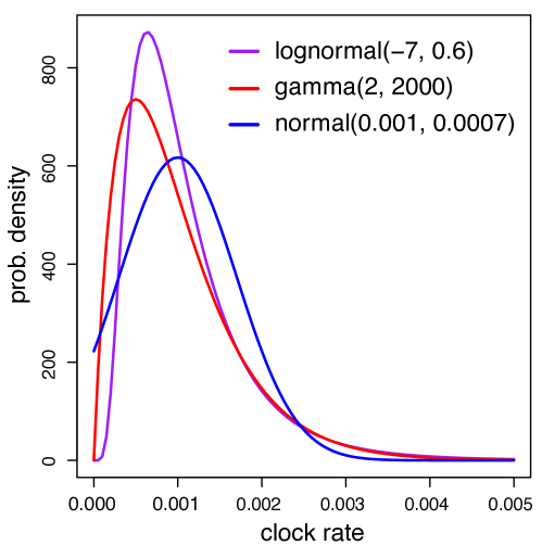
Figure 1: Probability density functions of normal, lognormal and gamma distributions, all with mean 0.001 and standard deviation 0.0007.

The relative clock rates, which are multiplied by the mean clock rate, vary differently along the branches of the tree in different models. The TK02 model assumes that the relative rate changes along the branches as Brownian motion on the log scale, starting from 1.0 (0.0 on the log scale) at the root. The rate at the end of a branch is lognormal distributed with mean equal to the rate at the beginning of the branch. Thus the rates at different branches are autocorrelated.

prset clockvarpr = tk02
prset tk02varpr = exp(1)

The IGR model assumes that the relative rate at each branch follows an independent gamma distribution with mean 1.0. The variance is proportional to the branch length.

prset clockvarpr = igr
prset igrvarpr = exp(10)

Note that when the relative rates are all fixed to 1.0 in the TK02 or IGR model, it becomes the strict clock model.

Before the total-evidence dating and node dating analyses, we first define the outgroup, fossil taxa, and some constraints for later use. Note these constraints are not enforced until we set topologypr explicitly (see below).

outgroup Raphidioptera
taxset fossils = Asioxyela Nigrimonticola Xyelotoma Undatoma Dahuratoma Cleistogaster Ghilarella Mesorussus Prosyntexis Pseudoxyelocerus
constraint HymenFossil = 2-.
constraint Hymenoptera = 2-10
constraint Holometabola = 1-10
constraint Tenthredinidae = 3-5
constraint CepSirOruApo = 7-10

3.5 Total-evidence dating

In the following, we assign priors for the fossils from the geological times. This is a typical step in total-evidence dating, where we calibrate the fossil taxa instead of the internal nodes of the tree.

calibrate
Asioxyela = unif(228,242)
Nigrimonticola = unif(152,163)
Xyelotoma = unif(152,163)
Undatoma = unif(145,152)
Dahuratoma = fixed(134)
Cleistogaster = unif(168,191)
Ghilarella = unif(113,125)
Mesorussus = unif(94,100)
Prosyntexis = unif(80,86)
Pseudoxyelocerus = fixed(182)
prset nodeagepr = calibrated

The last command nodeagepr is necessary to enable the calibrations.

The speciation, extinction, fossilization, and sampling process is explicitly modeled using the fossilized birth-death (FBD) process (Stadler, 2010; Heath et al., 2014; Gavryushkina et al., 2014; Zhang et al., 2016). Diversified sampling (Zhang et al., 2016) is arguably suitable for such higher-level taxa, which assumes exactly one representative extant taxa per clade descending from time $x_{cut}$ is sampled, and the fossils are sampled with a non-zero rate before $x_{cut}$ and zero after. A fossil can be either a tip or a sampled ancestor (Fig. 2).

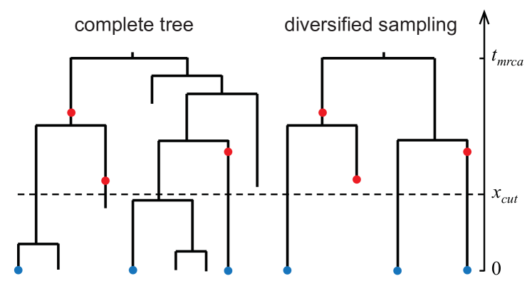
Figure 2: The fossilized birth-death (FBD) process and diversified sampling of extant taxa. Exactly one representative taxa per clade descending from time $x_{cut}$ is sampled (blue dots). The fossils are sampled with a constant rate between $t_{mrca}$ and $x_{cut}$ (red dots).

The model has four parameters: speciation rate $\lambda$, extinction rate $\mu$, fossil discovery rate $\psi$, and extant sample proportion $\rho$. For inference, we reparametrize the parameters as $d=\lambda-\mu$, $r=\mu/\lambda$, and $s=\psi/(\mu+\psi)$, so that the latter two parameters range from 0 to 1. $\rho$ is fixed to 0.0001, based on the living number of Hymenoptera at about $10/0.0001=100,000$.

prset brlenspr = clock:fossilization
prset samplestrat = diversity
prset sampleprob = 0.0001
prset speciationpr = exp(10)
prset extinctionpr = beta(1,1)
prset fossilizationpr = beta(1,1)
prset treeagepr = offsetexp(300,390)

The FBD prior is conditioned on the root age ($t_{mrca}$), so it is important to set it properly. Here we use an offset exponential distribution with minimal age 300 Ma and mean age 390 Ma. Several available probability densities all with mean 390 and minimal 300 are shown in Figure 3.

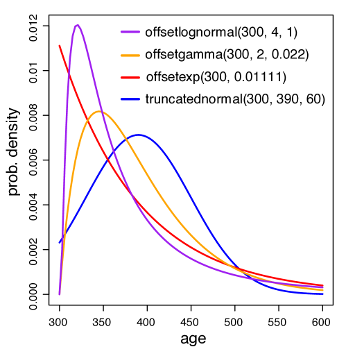
Figure 3: Probability density functions of offset lognormal, offset gamma, offset exponential, and truncated normal distributions, all with mean 390 and minimum 300.

An alternative tree prior that can be used in the total-evidence dating approach is the uniform prior (clock:uniform) (Ronquist et al., 2012a). It assumes that the internal nodes are draw from uniform distributions and the fossils are only tips of the tree (so-called tip dating). Same as the FBD prior, the uniform prior is also conditioned on the root age and requires setting treeagepr.

Using the molecular clock itself in this case cannot root the tree properly, we have to enable the constraint HymenFossil defined above. This forces the Hymenoptera with fossils to be a monophyletic group.

prset topologypr = constraint(HymenFossil)

For the Markov chain Monte Carlo (MCMC) (Metropolis et al., 1953; Hastings, 1970), we use two independent runs and four chains (one cold and three hot) per run for 500,000 iterations and sample every 100 iterations.

mcmcp nrun = 2 nchain = 4 ngen = 500000 samplefr = 100
mcmcp filename = hym.te printfr = 1000 diagnfr = 5000
mcmc

The output file names are hym.te.*. The chain states are printed to screen every 1000 iterations, and the convergence diagnostics is printed every 5000 iterations. The mcmc command executes the MCMC run.

While the MCMC is running, the iteration number, likelihood values, and average standard deviation of split frequencies (ASDSF) are printed to the screen. The ASDSF should be decreasing toward 0, indicating the tree topologies sampled from different runs are getting similar and converging to the same (stationary) distribution.

To summarize the parameters and trees after the MCMC, use

sump
sumt

By default, the first 25% samples are discarded as burnin. This can be adjusted according to the likelihood traces from the two runs. The effective sample size (ESS) also helps us to judge if sufficient MCMC samples are collected. Ideally, the ESS should be larger than 200 for all parameters. We may need to increase the chain length or adjust the priors to improve the estimates.

The consensus tree including all fossils is highly unresolved due to the uncertainty in the placement of the fossils. In order to display the node ages clearly, we can redraw an extant taxa tree by pruning the fossils. The output filename is changed to avoid overwriting the existing ones.

delete fossils
sumt output = hym.rf

3.6 Node dating

In node dating, we calibrate the internal nodes of the tree instead of assigning priors to the fossils. The morphological characters of the fossils are not used, thus we remove them.

delete fossils
exclude 24 130 168
calibrate
Tenthredinidae = offsetgamma(100,150,25)
CepSirOruApo = truncatednormal(140,175,25)
prset nodeagepr = calibrated

The birth-death prior under diversified sampling (Höhna et al., 2011) is used for the time tree. Compared to the FBD prior used above, there is no fossil sampling parameter in this case. The priors for the root age, speciation and extinction rates are not changed.

prset brlenspr = clock:birthdeath
prset samplestrat = diversity
prset sampleprob = 0.0001
prset speciationpr = exp(10)
prset extinctionpr = beta(1,1)
prset treeagepr = offsetexp(300,390)

The uniform tree prior (clock:uniform) is also applicable.

It is required to force the calibrated clade to be monophyletic and enable the constraints. The constraint Hymenoptera helps to root the tree properly.

prset topologypr = constraint(Hymenoptera, Tenthredinidae, CepSirOruApo)

The output filename is changed to avoid overwriting the existing ones. If the node dating analysis is continued after the total-evidence dating in the same MrBayes session, the starting values also need to be reset. The other settings are kept the same as in the total-evidence dating analysis.

mcmcp filename = hym.nd startp = reset startt = random

3.7 Non-clock analysis

Lastly, we run an analysis without molecular clock assumption and calibrations. The branch lengths are measured by genetic distance (expected substitutions per site). This is a typical analysis most people do using MrBayes. We do not use fossils, and do not constrain the topology so that they are uniformly distributed.

delete fossils
prset brlenspr = uncons:gammadir(1,1,1,1)
prset topologypr = uniform
mcmc filename = hym.un
sump
sumt

The prior for branch lengths is gamma-Dirichlet(1, 1, 1, 1) (Rannala et al., 2012; Zhang et al., 2012), which assigns gamma(1, 1) (i.e., exp(1)) for the tree length and uniform Dirichlet for the proportion of branch lengths. The compound Dirichlet prior was shown to help avoid overestimating the tree length (Zhang et al., 2012) and is now the default prior in MrBayes (since 3.2.3).

4 Results and Discussion

The posterior estimates of the parameters are summarized in separate files, which can be opened using a text editor. The information is also printed to the screen. The partition rate multipliers are in hym.*.pstat. The morphological (m{1}) and 16S (m{2}) partitions evolve at similar rate. The 1^st and 2^nd codon positions of Ef1$\alpha$ (m{3}) evolve much slower than the 3^rd codon positions (m{4}). Thus it is reasonable to take into account such significant rate variation across partitions.

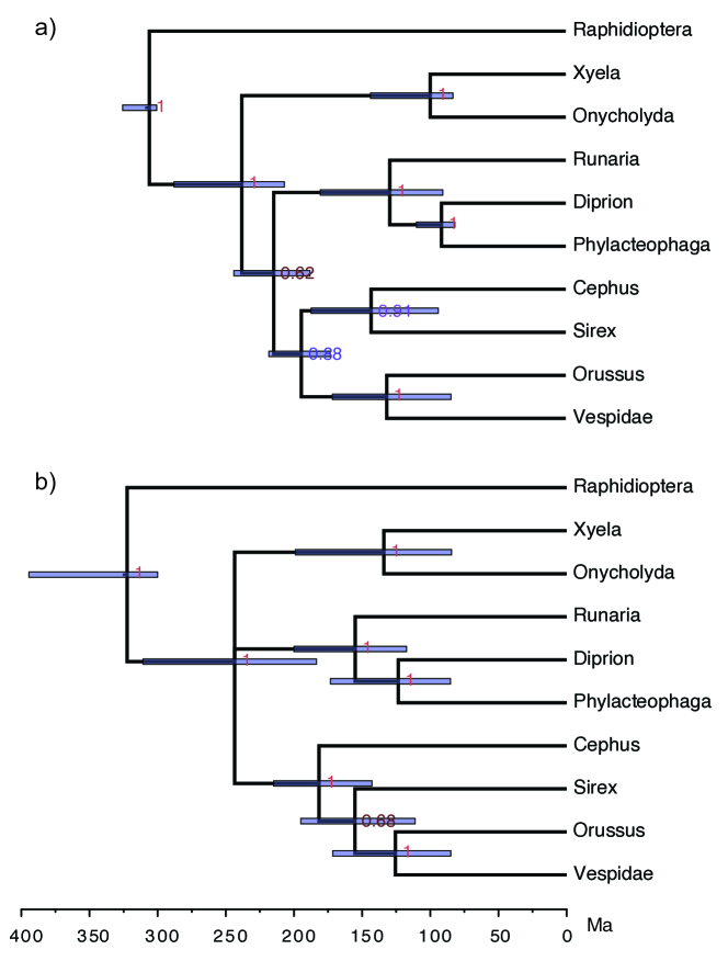
Figure 4: Majority-rule consensus trees of extant taxa from a) total-evidence dating and b) node dating, under diversified sampling and IGR model. The node heights are in the unit of million years and the error bars indicate the 95% HPD intervals. The numbers at the internal nodes are the posterior probabilities of the corresponding clades.

The majority-rule consensus trees are summarized in hym.*.con.tre, which can be visualized by FigTree (http://tree.bio.ed.ac.uk/software/figtree) or IcyTree (https://icytree.org). The node ages are also in hym.*.vstat, associated with the bipartition IDs in hym.*.parts. The root ID is 0 which includes all taxa, while the ID of Hymenoptera is that excludes the outgroup Raphidioptera (.*********). The extant taxa trees from total-evidence dating and node dating under diversified sampling and IGR model are shown in Figure 4. The topologies are the same in general, except for a clade with more uncertainties. The mean age of Hymenoptera (250 Ma) inferred from total-evidence dating is similar to that from node dating, with relatively narrower HPD interval.

The total-evidence dating approach models the fossilization and sampling process explicitly, and incorporates different sources of information from the fossil record while accounting for the uncertainty of fossil placement. In comparison, the node dating approach discards the fossil morphologies, and uses second interpretation of the fossil record as node calibrations. Total-evidence dating provides an ideal platform for exploring and further improving the models used for Bayesian molecular clock dating analysis.

Comparing the non-clock tree (Fig. 5) with the clock trees (Fig. 4), it is obvious that the evolutionary rate is not constant over time. The Xyela and Onycholyda branches evolve much slower than the Raphidioptera and Orussus/Vespidae clade, and there are indeed dramatic rate changes between adjacent branches. Thus the IGR relaxed clock model appears more suitable than the autocorrelated TK02 model, and it is not reasonable to assume a strict clock model. Further explorations, such as marginal likelihood estimation using stepping-stone sampling (Xie et al., 2011), could be carried out to compare the IGR with the TK02 model.

In conclusion, this study provides a brief overview and comparison of total-evidence dating and node dating analyses, and demonstrates the functionality of MrBayes using a dataset of Hymenoptera. For the analyses and discussion using the full data, please see Ronquist et al. (2012a); Zhang et al. (2016).

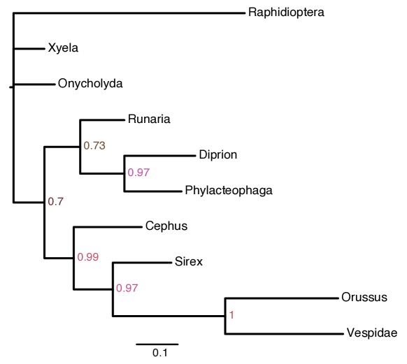
Figure 5: Majority-rule consensus tree of extant taxa from a non-clock analysis under the gamma-Dirichlet prior. The branch lengths are measured by expected substitutions per site. The numbers at the internal nodes are the posterior probabilities of the corresponding clades.

References

- Altekar et al. (2004) Altekar, G., S. Dwarkadas, J. P. Huelsenbeck, and F. Ronquist. 2004. Parallel Metropolis coupled Markov chain Monte Carlo for Bayesian phylogenetic inference. Bioinformatics 20:407–415.
- Ayres et al. (2012) Ayres, D. L., A. Darling, D. J. Zwickl, P. Beerli, M. T. Holder, P. O. Lewis, J. P. Huelsenbeck, F. Ronquist, D. L. Swofford, M. P. Cummings, A. Rambaut, and M. A. Suchard. 2012. BEAGLE: an application programming interface and high-performance computing library for statistical phylogenetics. Systematic Biology 61:170–173.
- Drummond et al. (2006) Drummond, A. J., S. Y. W. Ho, M. J. Phillips, and A. Rambaut. 2006. Relaxed phylogenetics and dating with confidence. PLoS Biology 4:e88.
- Gavryushkina et al. (2014) Gavryushkina, A., D. Welch, T. Stadler, and A. J. Drummond. 2014. Bayesian inference of sampled ancestor trees for epidemiology and fossil calibration. PLoS Computational Biology 10:e1003919.
- Hastings (1970) Hastings, W. K. 1970. Monte Carlo sampling methods using Markov chains and their applications. Biometrika 57:97–109.
- Heath et al. (2014) Heath, T. A., J. P. Huelsenbeck, and T. Stadler. 2014. The fossilized birth-death process for coherent calibration of divergence-time estimates. Proceedings of the National Academy of Sciences of the United States of America 111:E2957–66.
- Ho and Phillips (2009) Ho, S. Y. W. and M. J. Phillips. 2009. Accounting for calibration uncertainty in phylogenetic estimation of evolutionary divergence times. Systematic Biology 58:367–380.
- Höhna et al. (2011) Höhna, S., T. Stadler, F. Ronquist, and T. Britton. 2011. Inferring speciation and extinction rates under different sampling schemes. Molecular Biology and Evolution 28:2577–2589.
- Huelsenbeck et al. (2000) Huelsenbeck, J. P., B. Larget, and D. L. Swofford. 2000. A compound poisson process for relaxing the molecular clock. Genetics 154:1879–1892.
- Huelsenbeck and Ronquist (2001) Huelsenbeck, J. P. and F. Ronquist. 2001. MRBAYES: Bayesian inference of phylogenetic trees. Bioinformatics 17:754–755.
- Lakner et al. (2008) Lakner, C., P. van der Mark, J. P. Huelsenbeck, B. Larget, and F. Ronquist. 2008. Efficiency of Markov chain Monte Carlo tree proposals in Bayesian phylogenetics. Systematic Biology 57:86–103.
- Lepage et al. (2007) Lepage, T., D. Bryant, H. Philippe, and N. Lartillot. 2007. A general comparison of relaxed molecular clock models. Molecular Biology and Evolution 24:2669–2680.
- Lewis (2001) Lewis, P. O. 2001. A likelihood approach to estimating phylogeny from discrete morphological character data. Systematic Biology 50:913–925.
- Liu (2008) Liu, L. 2008. BEST: Bayesian estimation of species trees under the coalescent model. Bioinformatics 24:2542–2543.
- Liu et al. (2009) Liu, L., L. Yu, L. Kubatko, D. K. Pearl, and S. V. Edwards. 2009. Coalescent methods for estimating phylogenetic trees. Molecular Phylogenetics and Evolution 53:320–328.
- Metropolis et al. (1953) Metropolis, N., A. W. Rosenbluth, M. N. Rosenbluth, A. H. Teller, and E. Teller. 1953. Equation of state calculations by fast computing machines. Journal of Chemical Physics 21:1087–1092.
- Rannala et al. (2012) Rannala, B., T. Zhu, and Z. Yang. 2012. Tail paradox, partial identifiability, and influential priors in Bayesian branch length inference. Molecular Biology and Evolution 29:325–335.
- Ronquist and Huelsenbeck (2003) Ronquist, F. and J. P. Huelsenbeck. 2003. MrBayes 3: Bayesian phylogenetic inference under mixed models. Bioinformatics 19:1572–1574.
- Ronquist et al. (2012a) Ronquist, F., S. Klopfstein, L. Vilhelmsen, S. Schulmeister, D. L. Murray, and A. P. Rasnitsyn. 2012a. A total-evidence approach to dating with fossils, applied to the early radiation of the Hymenoptera. Systematic Biology 61:973–999.
- Ronquist et al. (2012b) Ronquist, F., M. Teslenko, P. van der Mark, D. L. Ayres, A. Darling, S. Höhna, B. Larget, L. Liu, M. A. Suchard, and J. P. Huelsenbeck. 2012b. MrBayes 3.2: efficient Bayesian phylogenetic inference and model choice across a large model space. Systematic Biology 61:539–542.
- Stadler (2010) Stadler, T. 2010. Sampling-through-time in birth-death trees. Journal of Theoretical Biology 267:396–404.
- Thorne and Kishino (2002) Thorne, J. L. and H. Kishino. 2002. Divergence time and evolutionary rate estimation with multilocus data. Systematic Biology 51:689–702.
- Van Noorden et al. (2014) Van Noorden, R., B. Maher, and R. Nuzzo. 2014. The top 100 papers. Nature 514:550–553.
- Xie et al. (2011) Xie, W., P. O. Lewis, Y. Fan, L. Kuo, and M.-H. Chen. 2011. Improving marginal likelihood estimation for Bayesian phylogenetic model selection. Systematic Biology 60:150–160.
- Yang (1994a) Yang, Z. 1994a. Estimating the pattern of nucleotide substitution. Journal of Molecular Evolution 39:105–111.
- Yang (1994b) Yang, Z. 1994b. Maximum likelihood phylogenetic estimation from DNA sequences with variable rates over sites: approximate methods. Journal of Molecular Evolution 39:306–314.
- Yang and Rannala (2006) Yang, Z. and B. Rannala. 2006. Bayesian estimation of species divergence times under a molecular clock using multiple fossil calibrations with soft bounds. Molecular Biology and Evolution 23:212–226.
- Zhang et al. (2012) Zhang, C., B. Rannala, and Z. Yang. 2012. Robustness of compound Dirichlet priors for Bayesian inference of branch lengths. Systematic Biology 61:779–784.
- Zhang et al. (2016) Zhang, C., T. Stadler, S. Klopfstein, T. A. Heath, and F. Ronquist. 2016. Total-evidence dating under the fossilized birth-death process. Systematic Biology 65:228–249.