Convergence of a Newton algorithm for semi-discrete optimal transport

Abstract.

A popular way to solve optimal transport problems numerically is to assume that the source probability measure is absolutely continuous while the target measure is finitely supported. We introduce a damped Newton’s algorithm in this setting, which is experimentally efficient, and we establish its global linear convergence for cost functions satisfying an assumption that appears in the regularity theory for optimal transport.

1. Introduction

Some problems in geometric optics or convex geometry can be recast as optimal transport problems between probability measures: this includes the far-field reflector antenna problem, Alexandrov’s Gaussian curvature prescription problem, etc. A popular way to solve these problems numerically is to assume that the source probability measure is absolutely continuous while the target measure is finitely supported. We refer to this setting as semi-discrete optimal transport. Among the several algorithms proposed to solve semi-discrete optimal transport problems, one currently needs to choose between algorithms that are slow but come with a convergence speed analysis [29, 8, 21] or algorithms that are much faster in practice but which come with no convergence guarantees [5, 27, 11, 22, 10]. Algorithms of the first kind rely on coordinate-wise increments and the number of iterations required to reach the solution up to an error of $\varepsilon$ is of order $N^{3}/\varepsilon$, where $N$ is the number of Dirac masses in the target measure. On the other hand, algorithms of the second kind typically rely on the formulation of the semi-discrete optimal transport problem as an unconstrained convex optimization problem which is solved using a Newton or quasi-Newton method.

The purpose of this article is to bridge this gap between theory and practice by introducing a damped Newton’s algorithm which is experimentally efficient and by proving the global convergence of this algorithm with optimal rates. The main assumptions is that the cost function satisfies a condition that appears in the regularity theory for optimal transport (the Ma-Trudinger-Wang condition) and that the support of the source density is connected in a quantitative way (it must satisfy a weighted Poincaré-Wirtinger inequality). In §1.7, we compare this algorithm and the convergence theorem to previous computational approaches to optimal transport.

1.1. Semi-discrete optimal transport

The source space is an open domain $\Omega$ of a $d$-dimensional Riemannian manifold, which we endow with the measure $\mathcal{H}_{g}^{d}$ induced by the Riemannian metric $g$ on the manifold. The target space is an (abstract) finite set $Y$. We are given a cost function $c$ on the product space $\Omega\times Y$, or equivalently a collection $(c(\cdot,y))_{y\in Y}$ of functions on $\Omega$. We assume that the functions $c(\cdot,y)$ are of class $\mathcal{C}^{1,1}$ on $\Omega$:

$$\forall y\in Y,~{}~{}c(\cdot,y)\in\mathcal{C}^{1,1}(\Omega).$$ (Reg)

Here $\mathcal{C}^{n,\alpha}(\Omega)$ denotes the class of functions which are $n$-times differentiable and whose $n$-th derivatives are $\alpha$-Hölder continuous. In particular, $\mathcal{C}^{0,\alpha}$ is the space of $\alpha$-Hölder continuous functions. We consider a compact subset $X$ of $\Omega$ and $\rho$ a probability density on $X$, i.e. such that $\rho\mathrm{d}\mathcal{H}^{d}$ is a probability measure. By an abuse of notation, we will often conflate the density $\rho$ with the measure $\rho\mathrm{d}\mathcal{H}^{d}$ itself. Note that the support of $\rho$ is contained in $X$, but we do not assume that it is actually equal to $X$. The push-forward of $\rho$ by a measurable map $T:X\to Y$ is the finitely supported measure $T_{\#}\rho=\sum_{y\in Y}\rho(T^{-1}(y))\delta_{y}$. The map $T$ is called a transport map between $\rho$ and a probability measure $\mu$ on $Y$ if $T_{\#}\rho=\mu$. The semi-discrete optimal transport problem consists in minimizing the transport cost over all transport maps between $\rho$ and $\mu$, that is

$$\min\left\{\int_{X}c(x,T(x))\rho(x)\mathrm{d}\mathcal{H}_{g}^{d}(x)\mid T:X\to Y\hbox{ s.t. }T_{\#}\rho=\mu\right\}.$$ (M)

This problem is an instance of Monge’s optimal transport problem, where the target measure is finitely supported. Kantorovich proposed a relaxed version of the problem (M) as an infinite dimensional linear programming problem over the space of probability measures with marginals $\rho$ and $\mu$.

1.2. Laguerre tessellation and economic interpretation

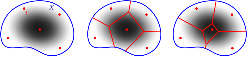
Figure 1. (Left) The domain $X$ (with boundary in blue) is endowed with a probability density pictured in grayscale representing the density of population in a city. The set $Y$ (in red) represents the location of bakeries. Here, $X,Y\subseteq\mathbb{R}^{2}$ and $c(x,y)=|x-y|^{2}$ (Middle) The Voronoi tessellation induced by the bakeries (Right) The Laguerre tessellation: the price of bread the bakery near the center of $X$ is higher than at the other bakeries, effectively shrinking its Laguerre cell.

In the semi-discrete setting, the dual of Kantorovich’s relaxation can be conveniently phrased using the notion of Laguerre tessellation. We start with an economic metaphor. Assume that the probability density $\rho$ describes the population distribution over a large city $X$, and that the finite set $Y$ describes the location of bakeries in the city. Customers living at a location $x$ in $X$ try to minimize the walking cost $c(x,y)$, resulting in a decomposition of the space called a Voronoi tessellation. The number of customers received by a bakery $y\in Y$ is equal to the integral of $\rho$ over its Voronoi cell, namely

$$\operatorname{Vor}_{y}:=\{x\in\Omega\mid\forall z\in Y,c(x,y)\leqslant c(x,z)\}.$$

If the price of bread is given by a function $\psi:Y\to\mathbb{R}$, customers living at location $x$ in $X$ make a compromise between walking cost and price by minimizing the sum $c(x,y)+\psi(y)$. This leads to the notion of Laguerre tessellation, whose cells are given by

$$\operatorname{Lag}_{y}(\psi):=\{x\in\Omega\mid\forall z\in Y,c(x,y)+\psi(y)\leqslant c(x,z)+\psi(z)\}.$$ (1.1)

When the sets $X$ and $Y$ are contained in $\mathbb{R}^{d}$ and the cost is the squared Euclidean distance, the computation of the Laguerre tessellation is a classical problem of computational geometry, for which there exists very efficient softwares, such as CGAL [1] or Geogram [2]. For other cost functions, one has to adapt the algorithms, as was done for the reflector cost on the sphere in [10]. The shape of the Voronoi and Laguerre tessellations is depicted in Figure 1.

We want the Laguerre cells to form a partition of $\Omega$ up to a negligible set. By the implicit function theorem, this will be the case if the following twist condition holds,

$$\forall x\in X,~{}~{}y\in Y\mapsto D_{x}c(x,y)\in T^{*}_{x}\Omega\hbox{ is injective,}$$ (Twist)

where $D_{x}$ denotes differentiation with respect to the first variable. The twist condition implies that for any prices $\psi$ on $Y$, the transport map induced by the Laguerre tessellation

$$T_{\psi}(x):=\arg\min_{y\in Y}(c(x,y)+\psi(y)),$$ (1.2)

is uniquely defined almost everywhere. It is easy to see (see Proposition 2.2), that for any function $\psi$ on $Y$, the map $T_{\psi}$ is an optimal transport map between $\rho$ and the pushforward measure $T_{\psi\#}\rho=\sum_{y\in Y}\rho(\operatorname{Lag}_{y}(\psi))\delta_{y}.$

1.3. Kantorovich’s functional

The map $T_{\psi}$ is an optimal transport map between $\rho$ and $T_{\psi\#}\rho$. Conversely, Theorem 1.1 below ensures that any semi-discrete optimal transport problem admits such a solution. In other words, for any probability density $\rho$ on $X$ and any probability measures $\mu$ on $Y$ there exists a function (price) $\psi$ on $Y$ such that $T_{\psi\#}\rho=\nu$. The proof of this theorem is an easy generalization of the proof given in [5] for the quadratic cost, but it is nonetheless included in Section 2 for the sake of completeness.

Here and after, we denote $(\mathbbold{1}_{y})_{y\in Y}$ the canonical basis of $\mathbb{R}^{Y}$, and $\left\|\cdot\right\|$ the Euclidean norm induced by this basis, while $\left\|\cdot\right\|_{g}$ will denote the norm induced by the Riemannian metric $g$ on either $T_{x}\Omega$ or $T^{*}_{x}\Omega$ (which will be clear from context). We will, slightly abusively, consider the space of probability measures $\mathcal{P}(Y)$ as a subset of $\mathbb{R}^{Y}$.

Theorem 1.1.

Assume (Reg) and (Twist), let $\rho$ be a bounded probability density on $X$ and $\nu=\sum_{y\in Y}\nu_{y}\mathbbold{1}_{y}$ in $\mathcal{P}(Y)$. Then, the functional $\Phi$

$$\Phi(\psi) :=\int_{X}(\min_{y\in Y}c(x,y)+\psi(y))\rho(x)\mathrm{d}\mathcal{H}_{g}^{d}(x)-\sum_{y\in Y}\psi(y)\nu_{y}$$

$$=\sum_{y\in Y}\int_{\operatorname{Lag}_{y}(\psi)}(c(x,y)+\psi(y))\rho(x)\mathrm{d}\mathcal{H}_{g}^{d}(x)-\sum_{y\in Y}\psi(y)\nu_{y}$$ (1.3)

is concave, $\mathcal{C}^{1}$-smooth, and its gradient is

$$\nabla\Phi(\psi)=\sum_{y\in Y}(\rho(\operatorname{Lag}_{y}(\psi))-\nu_{y})\mathbbold{1}_{y}.$$ (1.4)

Corollary 1.2.

The following statements are equivalent:

• $\psi:Y\to\mathbb{R}$ is a global maximizer of $\Phi$ ;

• $T_{\psi}$ is an optimal transport map between $\rho$ and $\nu$ ;

• $T_{\psi\#}\rho=\nu$, or equivalently,

  $$\forall y\in Y,~{}\rho(\operatorname{Lag}_{y}(\psi))=\nu_{y}$$ (MA)

We call Kantorovich’s functional the function $\Phi$ introduced in (1.3). Note that both this functional and its gradient are invariant by addition of a constant. The non-linear equation (MA) can be considered as a discrete version of the generalized Monge-Ampère equation that characterizes the solutions to optimal transport problems (see for instance Chapter 12 in [34]).

1.4. Damped Newton algorithm

We consider a simple damped Newton’s algorithm to solve semi-discrete optimal transport problem. This algorithm is very close to the one used by Mirebeau in [28]. To phrase this algorithm in a more general way, we introduce a notation for the measure of Laguerre cells: for $\psi\in\mathbb{R}^{Y}$ we set

$$G(\psi):=\sum_{y\in Y}G_{y}(\psi)\mathbbold{1}_{y}\hbox{ where }G_{y}(\psi)=\rho(\operatorname{Lag}_{y}(\psi)),$$ (1.5)

so that $\nabla\Phi(\psi)=G(\psi)-\nu$. In the algorithm (Algorithm 1), we denote by $A^{+}$ the pseudo-inverse of the matrix $A$.

Input:

A tolerance $\eta>0$ and an initial $\psi_{0}\in\mathbb{R}^{Y}$ such that

$$\varepsilon_{0}:=\frac{1}{2}\min\left[\min_{y\in Y}G_{y}(\psi_{0}),~{}\min_{y\in Y}\mu_{y}\right]>0.$$ (1.6)

While:

$\left\|G_{y}(\psi_{k})-\mu_{y}\right\|\geqslant\eta$

Step 1:

Compute $d_{k}=-\mathrm{D}G(\psi_{k})^{+}(G(\psi_{k})-\mu)$

Step 2:

Determine the minimum $\ell\in\mathbb{N}$ such that $\psi_{k}^{\ell}:=\psi_{k}+2^{-\ell}d_{k}$ satisfies

$$\left\{\begin{aligned} &\min_{y\in Y}G_{y}(\psi_{k}^{\ell})\geqslant\varepsilon_{0}\\ &\left\|G(\psi_{k}^{\ell})-\mu\right\|\leqslant(1-2^{-(\ell+1)})\left\|G(\psi_{k})-\mu\right\|\end{aligned}\right.$$

Step 3:

Set $\psi_{k+1}=\psi_{k}+2^{-\ell}d_{k}$ and $k\leftarrow k+1$.

Algorithm 1 Simple damped Newton’s algorithm

The goal of this article is to prove the global convergence of this damped Newton algorithm and to establish estimates on the speed of convergence. As shown in Proposition 6.1, the convergence of Algorithm 1 depends on the regularity and strong monotonicity of the map $G=\nabla\Phi$. As we will see, the regularity of $G$ will depend mostly on the geometry of the cost function and the regularity of the density. On the other hand, the strong monotonicity of $G$ will require a strong connectedness assumption on the support of $\rho$, in the form of a weighted Poincaré-Wirtinger inequality. Before stating our main theorem we give some indication about these intermediate regularity and monotonicity results and their assumptions.

1.5. Regularity of Kantorovich’s functional and MTW condition

In order to establish the convergence of a damped Newton algorithm for (MA), we need to study the $\mathcal{C}^{2,\alpha}$ regularity of Kantorovich’s functional $\Phi$. However, while $\mathcal{C}^{1}$ regularity of $\Phi$ follows rather easily from the (Twist) hypothesis (or even from weaker hypothesis, see Theorem 2.1), higher order regularity seems to depend on the geometry of the cost function in a more subtle manner. We found that a sufficient condition for the regularity of $\Phi$ is the Ma-Trudinger-Wang condition [26], which appeared naturally in the study of the regularity of optimal transport maps. We use a discretization of Loeper’s geometric reformulation of the Ma-Trundinger-Wang condition [23].

Definition 1.1 (Loeper’s condition).

The cost $c$ satisfies Loeper’s condition if for every $y$ in $Y$ there exists a convex open subset $\Omega_{y}$ of $\mathbb{R}^{d}$ and a $\mathcal{C}^{1,1}$ diffeomorphism $\exp^{c}_{y}:\Omega_{y}\to\Omega$ such that the functions

$$p\in\Omega_{y}\mapsto c(\exp^{c}_{y}p,y)-c(\exp^{c}_{y}p,z)$$ (QC)

are quasi-convex for all $z$ in $Y$. The map $\exp^{c}_{y}$ is called the $c$-exponential with respect to $y$, and the domain $\Omega_{y}$ is an exponential chart.

We comment here, that when $Y$ is a finite subset of a continuous space and $c$ satisfies conditions (Reg), (Twist), and (A3w) (which can be found on pages Reg, Twist, and A3w respectively), the $c$-exponential map defined in the usual sense in optimal transport theory (see Remarks 1.1 and 4.4) will satisfy what we call Loeper’s condition above. However, it will become apparent that for our purposes what is essential is the above quasi-convexity property and not the actual definition of $\exp^{c}_{y}$. Thus we will elect to use the notation $\exp^{c}_{y}$ even in cases when $Y$ is not a finite subset of a continuous space.

Definition 1.2 ($c$-Convexity).

Assuming Loeper’s condition, a subset $X$ of $\Omega$ is $c$-convex with respect to a point $y$ of $Y$ if its inverse image $(\exp_{y}^{c})^{-1}(X)$ is convex. The subset $X$ is said to be $c$-convex if it is $c$-convex with respect to every point $y$ in $Y$.

Note that by assumption, the domain $\Omega$ itself is $c$-convex. The connection between this discrete version of Loeper’s condition and the conditions used in the regularity theory for optimal transport is detailed in Remark 1.1. The (QC) condition implies the convexity of each Laguerre cell in its own exponential charts, namely $(\exp_{y}^{c})^{-1}(\operatorname{Lag}_{y}(\psi))$ is convex for every $y$ in $Y$. This plays a crucial role in the regularity of Kantorovich’s functional.

Theorem 1.3.

Assume (Reg), (Twist), and (QC). Let $X$ be a compact, $c$-convex subset of $\Omega$ and let $\rho$ in $\mathcal{P}^{\mathrm{ac}}(X)\cap\mathcal{C}^{0,\alpha}(X)$ for $\alpha$ in $(0,1]$. Then, Kantorovich’s functional is of class $\mathcal{C}^{2,\alpha}_{\text{loc}}$ on the set

$$\mathcal{K}^{+}:=\{\psi:Y\to\mathbb{R}\mid\forall y\in Y,~{}\rho(\operatorname{Lag}_{y}(\psi))>0\},$$ (1.7)

and its Hessian is given by

$$(z\neq y)\qquad \frac{\partial^{2}\Phi}{\partial\mathbbold{1}_{y}\partial\mathbbold{1}_{z}}(\psi)=\int_{\operatorname{Lag}_{y}(\psi)\cap\operatorname{Lag}_{z}(\psi)}\frac{\rho(x)}{\left\|D_{x}c(x,y)-D_{x}c(x,z)\right\|_{g}}\mathrm{d}\mathcal{H}_{g}^{d-1}(x),$$

$$\frac{\partial^{2}\Phi}{\partial\mathbbold{1}_{y}^{2}}(\psi)=-\sum_{z\in Y\setminus\{y\}}\frac{\partial^{2}\Phi}{\partial\mathbbold{1}_{y}\partial\mathbbold{1}_{z}}.$$ (1.8)

The proof of this theorem and a more precise statement are given in Section 4 (Theorem 4.1), showing that the $\mathcal{C}^{2,\alpha}$ estimate can be made uniform when the mass of the Laguerre cells is bounded from below by a positive constant.

Remark 1.1.

We remark that under certain assumptions on the cost $c$, our (QC) condition is implied by classical conditions introduced in a smooth setting by X.-N. Ma, N. Trudinger, and X.-J. Wang [26], which include the well known (MTW) or (A3) condition. See Remark 4.4 for more specifics.

There are a wide variety of known examples satisfying these conditions. Aside from the canonical example of the inner product on $\mathbb{R}^{n}\times\mathbb{R}^{n}$, and other costs on Euclidean spaces mentioned in [26, 33], there are the nonflat examples of Riemannian distance squared and $-\log\left\|x-y\right\|_{\mathbb{R}^{n+1}}$ on (a subset of) $\mathbb{S}^{n}\times\mathbb{S}^{n}$ (see [24]). The last cost is associated to the far-field reflector antenna problem. We refer the reader to [19, p. 1331] for a (more) comprehensive list of such costs.

1.6. Strong concavity of Kantorovich’s functional

As noted earlier, Kantorovich’s functional $\Phi$ cannot be strictly concave, since it is invariant under addition of a constant. This implies that the Hessian $\mathrm{D}^{2}\Phi$ has a zero eigenvalue corresponding to the constants. A more serious obstruction to the strict concavity of $\Phi$ at a point $\psi$ arises when the discrete graph induced by the Hessian (where two points are connected iff $\partial^{2}\Phi/\partial\mathbbold{1}_{y}\partial\mathbbold{1}_{z}(\psi)\neq 0$) is not connected. This can happen either because one of the Laguerre cells is empty (hence not connected to any neighbor) or if the support of the probability density $\rho$ is itself disconnected. In order to avoid the latter phenomena, we will require that $(X,\rho)$ satisfies a weighted $\mathrm{L}^{1}$ Poincaré-Wirtinger inequality.

Definition 1.3 (weighted Poincaré-Wirtinger).

A continuous probability density $\rho$ on a compact set $X\subseteq\Omega$ satisfies a weighted Poincaré-Wirtinger inequality with constant $C_{\mathrm{pw}}>0$ if for every $\mathcal{C}^{1}$ function $f$ on $X$,

$$\left\|f-\mathbb{E}_{\rho}(f)\right\|_{L^{1}(\rho)}\leqslant C_{\mathrm{pw}}\left\|\nabla f\right\|_{L^{1}(\rho)},$$ (PW)

where $\left\|h\right\|_{L^{1}(\rho)}:=\int_{X}|h(x)|\rho(x)\mathrm{d}\mathcal{H}_{g}^{d}(x)$ and $\mathbb{E}_{\rho}(f):=\int_{X}f(x)\rho(x)\mathrm{d}\mathcal{H}_{g}^{d}(x)$.

We denote $E_{Y}$ the orthogonal complement (in $\mathbb{R}^{Y}$) of the space of constant functions on $Y$, that is $E_{Y}:=\{\psi\in\mathbb{R}^{Y}\mid\sum_{y}\psi(y)=0\}.$ As before, $\mathcal{K}^{+}$ is the set of functions $\psi$ whose Laguerre cells all have positive mass.

Theorem 1.4.

Assume (Reg), (Twist), and (QC). Let $X$ be a compact, $c$-convex subset of $\Omega$, and $\rho$ be a continuous probability density on $X$ satisfying (PW). Then, Kantorovich’s functional $\Phi$ is strictly concave on $E_{Y}\cap\mathcal{K}^{+}$.

As before, a more quantitative statement is proven in Section 5 (Theorem 5.1), establishing strong concavity of $\Phi$ assuming that the mass of the Laguerre cells is bounded from below by a positive constant.

1.7. Convergence result

Putting Proposition 6.1, Theorem 1.3 and Theorem 1.4 together, we can prove the global convergence of the damped Newton algorithm for semi-discrete optimal transport (Algorithm 1) together with optimal convergence rates.

Theorem 1.5.

Assume (Reg), (Twist) and (QC) and also that

• The support of the probability density $\rho$ is included in a compact, $c$-convex subset $X$ of $\Omega$, and $\rho\in\mathcal{C}^{0,\alpha}(X)$ for $\alpha$ in $(0,1]$.

• $\rho$ has positive Poincaré-Wirtinger (PW) constant.

Then the damped Newton algorithm for semi-discrete optimal transport (Algorithm 1) converges globally with linear rate and locally with rate $1+\alpha$.

Remark 1.2.

This theorem makes no assumption about the convexity (or $c$-convexity) of the support of the source density $\rho$. Such cases are not handled by other numerical methods for Monge-Ampère equations [6, 24]. For completeness, we provide in Appendix A an explicit example of a radial measure on $\mathbb{R}^{d}$ whose support is an annulus but whose Poincaré-Wirtinger constant is nonetheless positive.

Remark 1.3.

The positive lower bound on the damping parameter ($\tau_{k}=2^{-\ell}$ in Algorithm 1) established in this theorem degrades as $N$ grows to infinity. It is plausible (but far from direct) that one could control this quantity when $N$ is large by a comparison to the continuous Monge-Ampère equation. The strong concavity estimate (Theorem 1.4) would then need to be replaced by uniform ellipticity estimates for the linearized Monge-Ampère equation, while the regularity estimate (Theorem 1.3) would be replaced by regularity estimates for solutions to the Monge-Ampère equation. We refer to Loeper and Rapetti [25] for an implementation of this ideas in a continuous setting. The space-discretization of their approach is open.

Comparison to previous work.

There exist a few other numerical methods relying on Newton’s algorithm for the resolution of the standard Monge-Ampère equation or for the quadratic optimal transport problem. Here, we highlight some of the differences between Algorithm 1 and Theorem 1.5 and these existing results. First, we note that many authors have reported the good behavior in practice of Newton’s or quasi-Newton’s methods for solving discretized Monge-Ampère equations or optimal transport problems [27, 11, 6]. Note however that none of these works contain convergence proofs for the Newton’s algorithm.

Loeper and Rapetti [25] (refined by Saumier, Agueh, and Khouider [31]) establish the global convergence of a damped Newton’s method for solving quadratic optimal transport on the torus, relying heavily on Caffarelli’s regularity theory. In particular, the convergence of the algorithm requires a positive lower bound on the probability densities, while this condition is not necessary for Theorem 1.5 (see Section 5 and Appendix A where we construct explicitly probability densities with non-convex support that still satisfy the hypothesis of Theorem 1.5). A second drawback on relying on the regularity theory for optimal transport is that the damping parameter, which is an input parameter of the algorithm used in [25], cannot be determined explicitly from the data. Third, the convergence proof is for continuous densities, and it seems difficult to adapt it to the space-discretized problem. On the positive side, it seems likely that the convergence proof of [25][31] can be adapted to cost functions satisfying the Ma-Trudinger-Wang condition (which is equivalent to Loeper’s condition (QC) that we also require).

Oliker and Prussner prove the local convergence of Newton’s method for finding Alexandrov’s solutions to the Monge-Ampère equation $\det\mathrm{D}^{2}u=\nu$ with Dirichlet boundary conditions, where $\nu$ is a finitely supported measure [29]. Global convergence for a damped Newton’s algorithm is established by Mirebeau [28] for a variant of Oliker and Prussner’s discretization, but without convergence rates. Theorem 1.5 can be seen as an extension of the strategy used by Mirebeau to optimal transport problems, which amounts to (a) replacing the Dirichlet boundary conditions with the second boundary value conditions from optimal transport (b) replacing the Lebesgue measure by more general probability densities and (c) changing the Monge-Ampère equation itself in order to deal with more general cost functions.

We also comment here that our result Theorem 5.1 answers a conjecture first raised by Gangbo and McCann, in the case when the cost function satisfies the Ma-Trudinger-Wang condition. In [15, Example 1.6], a numerical approach to the semi-discrete optimal transport problem is suggested by taking what is equivalent to the negative gradient flow of the Kantorovich function defined in (1.3) above. There, Gangbo and McCann conjecture that this gradient flow should converge, and our result of uniform concavity of the Kantorovich functional provides a positive answer to a quantitative strengthening of this conjecture, at least for costs, measures, and domains satisfying the assumptions of Theorem 5.1.

Finally, we note that the overall strategy for proving the convergence of Algorithm 1 (proving regularity then strict concavity of $\Phi$) shares features to the one used in [9] to study the relationship between highly anisotropic semi-discrete quadratic optimal transport and Knothe rearrangement.

Outline

In Section 2, we establish the differentiability of Kantorovich’s functional $\Phi$, adapting arguments from [5]. In Sections 3 and 4, we prove the (uniform) second-differentiability of Kantorovich’s functional when the cost function satisfies Loeper’s (QC) condition. Section 5 is devoted to the proof of uniform concavity of Kantorovich’s functional, when the probability density satisfies a Poincaré-Wirtinger inequality (PW). In Section 6, we combine these intermediate results to prove the convergence of the damped Newton’s algorithm (Theorem 1.5), and we present a numerical illustration. Appendix A presents an explicit construction of a probability density with non-convex support over $\mathbb{R}^{d}$ which satisfies the assumptions of Theorem 1.5. Appendix B contains the details of the proof of the main theorem of Section 4.

Acknowledgements

QM and BT would like to acknowledge the support of the French ANR through the grant ANR-16-CE40-0014 (MAGA). BT is also partially supported by LabEx PERSYVAL-Lab (ANR-11-LABX-0025-01).

2. Kantorovich’s functional

The purpose of this section is to present the variational formulation introduced in [5] for the semi-discrete optimal transport problem, adapting the arguments presented for the squared Euclidean cost in [5] to cost functions satisfying (Reg’) and (Twist’), which are weaker than the conditions (Reg) and (Twist) presented in the introduction:

$$\forall y\in Y,~{}~{}c(\cdot,y)\in\mathcal{C}^{0}(\Omega)$$ (Reg’)

$$\forall y\neq z\in Y,\ \forall t\in\mathbb{R},~{}~{}\mathcal{H}_{g}^{d}((c(\cdot,y)-c(\cdot,z))^{-1}(t))=0$$ (Twist’)

Note that under (Twist’), the map $T_{\varphi}:X\to Y$ defined by (1.2) is uniquely-defined $\mathcal{H}_{g}^{d}$–almost everywhere. Most of the results presented here are well known in the optimal transport literature, we include proofs for completeness.

Theorem 2.1.

Assume (Reg’) and (Twist’), and let $\rho$ be a bounded probability density on $X$ and $\nu=\sum_{y\in Y}\nu_{y}\delta_{y}$ be a probability measure over $Y$. Then, the functional $\Phi$ defined by (1.3) is concave, $\mathcal{C}^{1}$-smooth, and its gradient is given by (1.4).

The proof of Theorem 2.1 relies on Propositions 2.2 and 2.3.

Proposition 2.2.

For any $\psi:Y\to\mathbb{R}$, the map $T_{\psi}$ is an optimal transport map for the cost $c$ between any probability density $\rho$ on $\Omega$ and the pushforward measure $\nu:=T_{\psi\#}\rho$.

Proof.

Assume that $\nu=S_{\#}\rho$ where $S$ is a measurable map between $X$ and $Y$. Then, by definition of $T_{\psi}$ one has

$$\forall x\in X,~{}~{}c(x,T_{\psi}(x))+\psi(T_{\psi}(x))\leqslant c(x,S(x))+\psi(S(x)).$$

Multiplying this inequality by $\rho$ and integrating it over $X$ gives

$$\int_{X}(c(x,T_{\psi}(x))+\psi(T_{\psi}(x)))\rho(x)\mathrm{d}\mathcal{H}_{g}^{d}(x)\leqslant\int_{X}(c(x,S(x))+\psi(S(x)))\rho(x)\mathrm{d}\mathcal{H}_{g}^{d}(x)$$

Since $\nu=S_{\#}\rho=T_{\psi\#}\rho$, the change of variable formula gives

$$\int_{X}\psi(S(x))\rho(x)\mathrm{d}\mathcal{H}_{g}^{d}(x)=\int_{Y}\varphi(y)\mathrm{d}\nu=\int_{X}\psi(T_{\psi}(x))\rho(x)\mathrm{d}\mathcal{H}_{g}^{d}(x)$$

Substracting this equality from the inequality above shows that $T_{\psi}$ is optimal:

$$\int_{X}c(x,T_{\psi}(x))\rho(x)\mathrm{d}\mathcal{H}_{g}^{d}(x)\leqslant\int_{X}c(x,S(x))\rho(x)\mathrm{d}\mathcal{H}_{g}^{d}(x)\qed$$

Proposition 2.3.

Assume (Twist’) and (Reg’). Let $\rho$ be a probability density over a compact subset $X$ of $\Omega$. Then, the map $G:\mathbb{R}^{Y}\to\mathbb{R}^{Y}$ is continuous:

$$G(\psi)=\left(\rho(\operatorname{Lag}_{y}(\psi))\right)_{y\in Y}$$ (2.9)

Lemma 2.4.

Let $\rho$ be a probability density over a compact subset $X$ of $\Omega$, and let $f$ in $\mathcal{C}^{0}(X)$ be such that $\rho(f^{-1}(t))=0$ for all $t\in\mathbb{R}$. Then, the function $g:t\mapsto\rho(f^{-1}((-\infty,t]))$ is continuous.

Proof.

We consider the function $h(t)=\rho(f^{-1}((-\infty,t)))$. By hypothesis, $g(t)-h(t)=\rho(f^{-1}(t))=0$. Moreover, using Lebesgue’s monotone convergence theorem one easily sees that $g$ (resp. $h$) is right-continuous (resp. left-continuous). This concludes the proof ∎

Proof of Proposition 2.3.

Proving the continuity of $G$ amounts to proving the continuity of the functions $G_{y}(\psi):=\rho(\operatorname{Lag}_{y}(\psi))$ for any $y$ in $Y$. Fix $y$ in $Y$ and remark that by definition, $\operatorname{Lag}_{y}(\psi)=\bigcap_{z\neq y\in Y}H_{z}(\psi)$ where

$$H_{z}(\psi):=\{x\in X\mid c(x,y)+\psi(y)\leqslant c(x,z)+\psi(z)\}.$$

Denoting $A\Delta B$ the symmetric difference of two sets, we have the following inequalities

$$\left|G_{y}(\psi)-G_{y}(\varphi)\right|\leqslant\rho(\operatorname{Lag}_{y}(\psi)\Delta\operatorname{Lag}_{y}(\varphi))\leqslant\sum_{z\in Y\setminus\{y\}}\rho(H_{z}(\psi)\Delta H_{z}(\varphi)).$$ (2.10)

Fix $z\neq y\in Y$, and denote $f=c(\cdot,y)-c(\cdot,z)$. Then,

$$H_{z}(\psi)\Delta H_{z}(\varphi)\subseteq f^{-1}([\psi(z)-\psi(y),\varphi(z)-\varphi(y)]).$$

Here and after, we use the convention that $[a,b]=[\min\{a,b\},\max\{a,b\}]$. By (Twist’) and Lemma 2.4 we know that $\lim_{\varphi\to\psi}\rho(H_{z}(\psi)\Delta H_{z}(\varphi))=0,$ which with (2.10) concludes the proof. ∎

2.1. Proof of Theorem 1.1

We simultaneously show that the functional is concave and compute its gradient. For any function $\psi$ on $Y$ and any measurable map $T:X\to Y$, one has $\min_{y\in Y}(c(x,y)+\psi(y))\leqslant c(y,T(y))+\psi(T(y))$, which by integration gives

$$\Phi(\psi)\leqslant\int_{X}(c(x,T(x))+\psi(T(x)))\rho(x)\mathrm{d}\mathcal{H}_{g}^{d}(x)-\sum_{y\in Y}\psi(y)\nu_{y}.$$ (2.11)

Moreover, equality holds when $T=T_{\psi}$. Taking another function $\varphi$ on $Y$ and setting $T=T_{\varphi}$ in Equation (2.11) gives

$$\Phi(\psi)\leqslant\Phi(\varphi)+\langle G(\varphi)-\nu\mid\psi-\varphi\rangle,$$

where $G$ is defined as in the statement of Proposition 2.3. This proves that the superdifferential $\partial^{+}\Phi(\varphi)$ contains $G(\varphi)-\nu$, thus establishing the concavity of $\Phi$ and its differentiability almost everywhere. It is known that the supergradient $\partial^{+}\Phi(\varphi)$ is characterized by [30, Theorem 25.6]

$$\partial^{+}\Phi(\varphi)=\mathrm{conv}\left\{\lim_{n\to\infty}\nabla\Phi(\varphi_{n})\mid(\varphi_{n})\in S\right\},$$

where $\mathrm{conv}$ denotes the convex envelope and $S$ the set of sequences $(\varphi_{n})$ converging to $\varphi$ such that $\Phi$ is differentiable at $\varphi_{n}$. By Proposition 2.3, the map $G$ is continuous, meaning that we have constructed a continuous selection of a supergradient in the superdifferential of the concave function $\Phi$

$$\partial^{+}\Phi(\varphi)=\mathrm{conv}\left\{\lim_{n\to\infty}\nabla\Phi(\varphi_{n})\right\}=\mathrm{conv}\left\{\lim_{n\to\infty}G(\varphi_{n})-\nu\right\}=\{G(\varphi)-\nu\}.$$

This proves that $\Phi$ is $\mathcal{C}^{1}$, and that $\nabla\Phi(\varphi)=G(\varphi)-\nu$.

3. Local regularity in a $c$-exponential chart

The results presented in this section constitute an intermediate step in the proof of $\mathcal{C}^{2,\alpha}$ regularity of Kantorovich’s functional. Let $\hat{X}$ be a compact, convex subset of $\mathbb{R}^{d}$ and $f_{1},\ldots,f_{N}$ be $\mathcal{C}^{1,1}$ functions on $\hat{X}$ which are quasi-convex, meaning that for any scalar $\lambda\in\mathbb{R}$ the closed sublevel sets $K_{i}(\lambda):=f_{i}^{-1}([-\infty,\lambda])$ are convex. Let $\hat{\rho}$ be a continuous probability density over $\hat{X}$. The purpose of this section is to give sufficient conditions to ensure the regularity of the following function $\hat{G}$ near the origin of $\mathbb{R}^{N}$:

$$\hat{G}:\bm{\lambda}\in\mathbb{R}^{N}\mapsto\int_{K(\bm{\lambda})}\hat{\rho}(x)\mathrm{d}\mathcal{H}^{d}(x),$$ (3.12)

$$\hbox{where }K(\bm{\lambda}):=\bigcap_{i=1}^{N}K_{i}(\lambda_{i})=\{x\in\hat{X}\mid\forall i\in\{1,\ldots,N\},~{}f_{i}(x)\leqslant\lambda_{i}\}.$$

3.1. Assumptions and statement of the theorem.

We will impose two conditions on the functions $(f_{i})_{1\leqslant i\leqslant N}$. As we will see in Section 4, both conditions are satisfied when these functions $(f_{i})$ are constructed from a semi-discrete optimal transport transport problem whose cost function satisfy Loeper’s condition (see Definition 1.1).

Non-degeneracy

The functions $(f_{i})$ satisfy the nondegeneracy condition if the norm of their gradients is bounded from below:

$$\varepsilon_{nd}:=\min_{1\leqslant i\leqslant N}\min_{\hat{X}}\left\|\nabla f_{i}\right\|>0.$$ (ND)

This condition is necessary for the continuity of the map $\hat{G}$ even when $N=1$.

Transversality

The boundary of the convex set $K(\bm{\lambda})$ can be decomposed into $N+1$ facets, namely $(K(\bm{\lambda})\cap\partial K_{i}(\lambda_{i}))_{1\leqslant i\leqslant N}$ and $K(\bm{\lambda})\cap\partial\hat{X}$. The purpose of the transversality condition we consider is to ensure that the angle between adjacent facets is bounded from below when $\bm{\lambda}$ remains close to some fixed vector $\bm{\lambda}_{0}$.

Definition 3.1 (Normal cone).

Let $K$ be a convex compact set of $\mathbb{R}^{d}$. The normal cone to $K$ at a point $x$ in $K$ is the set

$$\mathcal{N}_{x}K=\{v\in\mathbb{R}^{d}\mid\forall y\in K,~{}\langle y-x\mid v\rangle\leqslant 0\},$$ (3.13)

and its elements are said to be normal to $K$ at $x$.

Definition 3.2 (Transversality).

The family of functions $(f_{i})$ satisfy the transversality condition near $\bm{\lambda}_{0}$ if there exists positive constants $\varepsilon_{tr}$ and $T_{tr}\leqslant 1$ such that for every $\bm{\lambda}$ in $\mathbb{R}^{N}$ satisfying $\left\|\bm{\lambda}-\bm{\lambda_{0}}\right\|_{\infty}\leqslant T_{tr}$ for the usual $\ell^{\infty}$ norm on $\mathbb{R}^{N}$ and every point $x$ in $\partial K(\bm{\lambda})$ one has,

$$\hbox{ if }\exists i\neq j\in\{1,\ldots,N\}\hbox{ s.t. }f_{i}(x)=\lambda_{i}\hbox{ and }f_{j}(x)=\lambda_{j},$$ (T)

$$\hskip 113.81102pt\hbox{ then, }\left(\frac{\langle\nabla f_{i}(x)\mid\nabla f_{j}(x)\rangle}{\left\|\nabla f_{i}(x)\right\|\left\|\nabla f_{j}(x)\right\|}\right)^{2}\leqslant 1-\varepsilon^{2}_{tr}$$

$$\hbox{ if }\exists i\in\{1,\ldots,N\}\hbox{ s.t. }f_{i}(x)=\lambda_{i}\hbox{ and }x\in\partial\hat{X},$$

$$\hskip 99.58464pt\hbox{ then, }\forall u\in\mathcal{N}_{x}\hat{X},~{}\left(\frac{\langle u\mid\nabla f_{j}(x)\rangle}{\left\|u\right\|\left\|\nabla f_{j}(x)\right\|}\right)^{2}\leqslant 1-\varepsilon^{2}_{tr},$$

Note that $\partial\hat{X}$ is smooth at $x$, $\mathcal{N}_{x}\hat{X}$ is the ray spanned by the exterior normal to $\hat{X}$ at $x$.

Theorem 3.1.

Assume that the functions satisfy the non-degeneracy condition (ND) and the transversality condition (T) near $\bm{\lambda_{0}}$. Let $\hat{\rho}$ be a $\mathcal{C}^{0,\alpha}$ probability density on $\hat{X}$. Then, the map $\hat{G}$ defined in (3.12) is of class $\mathcal{C}^{1,\alpha}$ on the cube $Q:=\bm{\lambda_{0}}+[-T_{tr},T_{tr}]^{N}$ and has partial derivatives given by

$$\frac{\partial\hat{G}}{\partial\lambda_{i}}(\bm{\lambda})=\int_{K({\bm{\lambda}})\cap\partial K_{i}({\bm{\lambda}})}\frac{\hat{\rho}(x)}{\left\|\nabla f_{i}(x)\right\|}\mathrm{d}\mathcal{H}^{d-1}(x).$$ (3.14)

In addition, the norm $\left\|\hat{G}\right\|_{\mathcal{C}^{1,\alpha}(Q)}$ is bounded by a constant depending only on $\varepsilon_{tr},\varepsilon_{nd},\left\|\hat{\rho}\right\|_{\mathcal{C}^{0,\alpha}(\hat{X})}$, on the diameter of $\hat{X}$ and on

$$C_{M}:=\max_{1\leqslant i\leqslant N}\left\|\nabla f_{i}\right\|_{\infty}\qquad C_{L}:=\max_{1\leqslant i\leqslant N}\left\|\nabla f_{i}\right\|_{\operatorname{Lip}(\hat{X})}.$$

Note that the $\mathcal{C}^{1,\alpha}$ constant of $\hat{G}$ depends on the transversality constant $\varepsilon_{tr}$ but that it does not depend on $T_{tr}$.

3.2. Sketch of proof

The correct expression for the partial derivatives of $\hat{G}$, given by equation (3.14), can easily be guessed by applying the co-area formula. The non-degeneracy condition then ensures that the denominator in this expression does not vanish. What is more delicate is to prove that these partial derivatives are $\alpha$-Hölder, with a uniform estimate on the $\alpha$-Hölder norm. A second application of the co-area formula on the manifold $f_{i}^{-1}(\lambda_{i})$ suggests that for $j\neq i$ one should have,

$$\left|\frac{\partial}{\partial\lambda_{j}}\int_{K({\bm{\lambda}})\cap\partial K_{i}({\bm{\lambda}})}\frac{\hat{\rho}(x)}{\left\|\nabla f_{i}(x)\right\|}\mathrm{d}\mathcal{H}^{d-1}(x)\right|\leqslant C\mathcal{H}^{d-2}(K({\bm{\lambda}})\cap\partial K_{i}({\bm{\lambda}})\cap\partial K_{j}({\bm{\lambda}})),$$

under the assumption that the density $\hat{\rho}$ is $\mathcal{C}^{1}$ and the facet $K({\bm{\lambda}})\cap\partial K_{i}({\bm{\lambda}})$ does not intersect $\partial\hat{X}$. It will turn out that, thanks to the transversality hypothesis, the $\mathcal{H}^{d-2}$-measure of the union $\Sigma(\bm{\lambda})$ of these facets can be bounded uniformly:

$$\Sigma(\bm{\lambda})=\bigcup_{1\leqslant i\leqslant N}(K(\bm{\lambda})\cap\partial\hat{X}\cap\partial K_{i}(\lambda_{i}))\cup\bigcup_{1\leqslant i<j\leqslant N}(K(\bm{\lambda})\cap\partial K_{i}(\lambda_{i})\cap\partial K_{j}(\lambda_{j})).$$

Note also that equivalently, a point $x$ belongs to the singular set $\Sigma(\bm{\lambda})$ if and only if it satisfies one of the assumptions in (T). In the next subsection, we prove an upper bound on $\mathcal{H}^{d-2}(\Sigma(\bm{\lambda}))$ (see Proposition 3.2). The proof of Theorem 3.1 follows from this upper bound and from several applications of the co-area formula. Since it is elementary but quite long, we have postponed the proof of the theorem itself to Appendix B.

3.3. A control on the $(d-2)$–Hausdorff measure of singular points

In this section, we prove that the transversality condition (T) and the quasi-convexity of the functions $(f_{i})$ imply a uniform upper bound on the $(d-2)$–Hausdorff measure of $\Sigma(\bm{\lambda})$.

Proposition 3.2.

Assuming the transversality condition (T), there exists a constant depending only on $d$ and $\operatorname{diam}(\hat{X})$ such that for every $\left\|\bm{\lambda}\right\|_{\infty}\leqslant T_{tr}$,

$$\mathcal{H}^{d-2}(\Sigma(\bm{\lambda}))\leqslant C(d,\operatorname{diam}(\hat{X}))\cdot\frac{1}{\varepsilon_{tr}}.$$

We will deduce this proposition from a general upper bound on the $(d-2)$–Hausdorff measure of the set of $\tau$–singular points of a compact convex body. A more general and quantitative version of this bound can be found in [18]. We provide below a straightforward and easy proof based on the notions of packing and covering numbers.

Proposition 3.3.

Let $K$ be a convex, compact set of $\mathbb{R}^{d}$ and $\tau>0$. Then,

$$\mathcal{H}^{d-2}(\mathrm{Sing}(K,\tau))\leqslant C(d,\operatorname{diam}(K))\ \frac{1}{\tau},$$

where $\mathrm{Sing}(K,\tau):=\{x\in\partial K\mid\exists u,v\in\mathcal{N}_{x}(K)\cap\mathbb{S}^{d-1},~{}~{}\langle u\mid v\rangle^{2}\leqslant 1-\tau^{2}\}.$

Recall that the covering number $\mathrm{Cov}(K,\eta)$ of a subset $K\subseteq\mathbb{R}^{d}$ is the minimum number of Euclidean balls of radius $\eta$ required to cover $K$. The packing number of a subset $K$ is given by

$$\mathrm{Pack}(K,\eta):=\max\{\mathrm{Card}(X)\mid X\subseteq K\hbox{ and }\forall x\neq y\in X,\left\|x-y\right\|\geqslant\eta\}.$$

We will use the following comparisons between covering and packing numbers:

$$\mathrm{Cov}(K,\eta)\leqslant\mathrm{Pack}(K,\eta)\leqslant\mathrm{Cov}(K,\frac{\eta}{2}).$$ (3.15)

Proof of Proposition 3.3.

The proof consists in comparing a lower bound and an upper bound of the packing number of the set

$$U:=\{(x,n)\in\mathbb{R}^{d}\times\mathbb{S}^{d-1}\mid x\in\mathrm{Sing}(K,\tau)\mbox{ and }n\in\mathcal{N}_{x}(K)\}.$$

Step 1. We first calculate an upper bound on the covering number of the unit bundle $\mathcal{U}K:=\{(x,n)\in\partial K\times\mathbb{S}^{d-1}\mid n\in\mathcal{N}_{x}K\}$. Given a positive radius $r$, we denote by $K^{r}$ the set of points that are within distance $r$ of $K$. By convexity, the projection map $\mathrm{p}_{K}:\mathbb{R}^{d}\to K$, mapping a point to its orthogonal projection on $K$, is well defined and $1$-Lipschitz. We consider

$$\pi:\partial K^{r} \to\mathcal{U}(K)$$

$$x \mapsto\left(\mathrm{p}_{K}(x),\frac{x-\mathrm{p}_{K}(x)}{\left\|x-\mathrm{p}_{K}(x)\right\|}\right)$$

The map $\pi$ is surjective and has Lipschitz constant $L:=\sqrt{1+4/r^{2}}$. We deduce an upper bound on covering number of $\mathcal{U}K$ from the covering number of the level set $\partial K^{r}$:

$$\mathrm{Cov}(\mathcal{U}(K),\varepsilon)\leqslant\mathrm{Cov}\left(\partial K^{r},\frac{\varepsilon}{L}\right).$$

Now, consider a sphere $S$ with diameter $2\operatorname{diam}(K)$ that encloses the tubular neighborhood $K^{r}$ with $r:=\operatorname{diam}(K)$. The projection map $\mathrm{p}_{K^{r}}$ is $1$-Lipschitz, and $\mathrm{p}_{K^{r}}(S)=\partial K^{r}$. Using the same argument as above, we have:

$$\mathrm{Cov}\left(\partial K^{r},\eta\right)\leqslant\mathrm{Cov}(S,\eta)\leqslant C(d)\cdot(\operatorname{diam}(K)/\eta)^{d-1}.$$

Combining these bounds with the inclusion $U\subseteq\mathcal{U}(K)$ gives us

$$\mathrm{Cov}(U,\varepsilon)\leqslant\frac{C(d,\operatorname{diam}(K))}{\varepsilon^{d-1}}.$$ (3.16)

Step 2. We now establish a lower bound for $\mathrm{Pack}(U,2\varepsilon)$. Let $x$ be a $\tau$-singular point and $u,v$ be two unit vectors such that $\langle u\mid v\rangle^{2}\leqslant 1-\tau^{2}$. This implies that $\mathcal{N}_{x}K\cap\mathbb{S}^{d-1}$ contains a spherical geodesic segment of length at least $C\cdot\tau$, giving us a lower bound on the packing number of $\mathcal{N}_{x}K\cap\mathbb{S}^{d-1}$, namely $\mathrm{Pack}(\mathcal{N}_{x}K\cap\mathbb{S}^{d-1},\eta)\geqslant C\cdot\tau/\eta$. Now, let $X$ be a maximal set in the definition of the packing number $\mathrm{Pack}(\mathrm{Sing}(K,\tau),2\varepsilon)$ and for every $x\in X$, let $Y_{x}$ be a maximal set in the definition of the packing number $\mathrm{Pack}(\mathcal{N}_{x}(K)\cap\mathbb{S}^{d-1},2\varepsilon)$, so that $\operatorname{Card}(Y_{x})\geqslant C\cdot\tau/\varepsilon$. Then, the set $Z:=\{(x,y)\mid x\in X,~{}y\in Y_{x}\}$ is a $2\varepsilon$ packing of $U$, and the cardinality of this set is bounded from below by $C\cdot\operatorname{Card}(X)\cdot\tau/\varepsilon$. This gives

$$\mathrm{Pack}(U,2\varepsilon)\geqslant C\cdot\mathrm{Pack}(\mathrm{Sing}(K,\tau),2\varepsilon)\cdot\tau/\varepsilon.$$ (3.17)

Step 3. Combining Equations (3.16), (3.17) and the comparison between packing and covering numbers (3.15), we get

$$\mathrm{Pack}(\mathrm{Sing}(K,\tau),2\varepsilon) \leqslant\frac{C(d,\operatorname{diam}(K))}{\tau\varepsilon^{d-2}}.$$

Using the comparison between packing and covering numbers, this means that we can cover $\mathrm{Sing}(K,\tau)$ with $N_{\varepsilon}$ balls of radius $\varepsilon$, such that $N_{\varepsilon}\leqslant C(d,\operatorname{diam}(K))/(\tau\varepsilon^{d-2})$. By definition of the Hausdorff measure, we have

$$\mathcal{H}^{d-2}(\mathrm{Sing}(K,\tau))\leqslant\liminf_{\varepsilon\to 0}N_{\varepsilon}\varepsilon^{d-2}\leqslant C(d,\operatorname{diam}(K))\frac{1}{\tau}.\qed$$

Proof of Proposition 3.2.

Given $\left\|\bm{\lambda}\right\|_{\infty}\leqslant T_{tr}$, the transversality condition (T) implies

$$\forall x\in\Sigma(\bm{\lambda}),~{}~{}\exists u,v\in\mathcal{N}_{x}K(\bm{\lambda}),~{}~{}\left(\frac{\langle u\mid v\rangle}{\left\|u\right\|\left\|v\right\|}\right)^{2}\leqslant 1-\varepsilon_{tr}^{2},$$

where $\mathcal{N}_{x}K(\bm{\lambda})$ is the normal cone to the convex set $K(\bm{\lambda})$ at $x$ (see (3.13)). This implies that $\Sigma(\bm{\lambda})$ is included in the set $\mathrm{Sing}(K(\bm{\lambda}),\varepsilon_{tr})$ of $\tau$-singular points with $\tau=\varepsilon_{tr}$. The conclusion then follows from Proposition 3.3. ∎

4. $\mathcal{C}^{2,\alpha}$ regularity of Kantorovich’s functional

This section is devoted to the proof of the following regularity result. Recall that the conditions (Reg), (Twist), and (QC) are defined in the introduction, respectively on pages Reg, Twist, and QC.

Theorem 4.1.

Assume (Reg), (Twist), and (QC). Let $X$ be a compact, $c$-convex subset of $\Omega$ and $\rho$ in $\mathcal{P}^{\mathrm{ac}}(X)\cap\mathcal{C}^{0,\alpha}(X)$ for $\alpha$ in $(0,1]$. Then, the Kantorovich’s functional $\Phi$ is uniformly $\mathcal{C}^{2,\alpha}$ on the set

$$\mathcal{K}^{\varepsilon}:=\{\psi:Y\to\mathbb{R}\mid\forall y\in Y,~{}\rho(\operatorname{Lag}_{y}(\psi))>\varepsilon\}$$ (4.18)

and its Hessian is given by (1.8). In addition, the $\mathcal{C}^{2,\alpha}$ norm of the restriction of $\Phi$ to $\mathcal{K}^{\varepsilon}$ depends only on $\left\|\rho\right\|_{\infty}$, $\varepsilon$, $\operatorname{diam}(X)$, and the constants defined in Remark 4.1 below.

For the remainder of the section, for any point $y$ in $Y$, we will denote $X_{y}=(\exp_{y}^{c})^{-1}(X)\subseteq\mathbb{R}^{d}$ the inverse image of the domain $X$ in the exponential chart at $y$. The set $X_{y}$ is convex by $c$-concavity of $X$. We consider the functions

$$f_{z,y}:p\in X_{y}\mapsto c(\exp_{y}^{c}(p),y)-c(\exp_{y}^{c}(p),z),$$

which are quasi-concave by (QC). The main difficulty in deducing Theorem 4.1 from Theorem 3.1 is in establishing the quantitative transversality condition (T) introduced on p. T for the family of functions $(f_{z,y})_{z\in Y\setminus\{y\}}$.

Remark 4.1 (Constants).

The $\mathcal{C}^{2,\alpha}$ norm of the restriction of $\Phi$ to $\mathcal{K}^{\varepsilon}$ explicitely depends on the following constants, whose finiteness (or positivity) follows from the compactness of the domain $X$, from the finiteness of the set $Y$ and from the conditions (Reg), (Twist), and (QC):

$$\varepsilon_{tw} :=\min_{x\in X}\min_{y,z\in Y\atop{y\neq z}}\left\|D_{x}c(x,y)-D_{c}(x,z)\right\|_{g}>0$$

$$C_{\nabla} :=\max_{(x,y)\in X\times Y}\left\|D_{x}c(x,y)\right\|_{g}<+\infty$$

$$C_{\mathrm{exp}} :=\max_{y\in Y}\max\left\{\left\|\exp_{y}^{c}\right\|_{\operatorname{Lip}(X_{y})},\left\|(\exp_{y}^{c})^{-1}\right\|_{\operatorname{Lip}(X)}\right\}<+\infty,$$ (4.19)

where we recall that $X_{y}:=\exp_{y}^{-1}(X)$. Our estimates will also rely on the following constants involving the differential of the exponential maps. As before, the tangent spaces $\mathrm{T}_{x}\Omega$ are endowed with the Riemannian metric $g$ from $\Omega$. We set:

$$C_{\mathrm{cond}} :=\max_{y\in Y}\max_{p\in X_{y}}\operatorname{cond}(\left.\mathrm{D}\exp_{y}^{c}\right|_{p}),$$

$$C_{\mathrm{det}} :=\max_{y\in Y}\left\|\det(\mathrm{D}\exp_{y}^{c})\right\|_{\operatorname{Lip}(X_{y})},$$

where $\operatorname{cond}(A)$ is the condition number of a linear transform $A$ between finite dimensional normed spaces and $\det(A)$ is the determinant of $A$ with respect to orthornormal bases. The quantitative transversality estimates involve all the above constants in an explicit way, see (4.31).

Remark 4.2.

Even in the Euclidean case, one needs a lower bound on the volume of Laguerre cells in order to establish the second-differentiability of the functional $\Phi$. Indeed, let $y_{\pm}=\pm 1$, let $y_{0}=0$, $Y=\{y_{-},y_{0},y_{+}\}\subseteq\mathbb{R}$. Consider the cost $c(x,y)=-xy$, and the density $\rho=1$ on $X=[-\frac{1}{2},\frac{1}{2}]$. Let $\varphi_{\tau}\in\mathbb{R}^{Y}$ be defined by $\varphi(y_{\pm})=1/2$ and $\varphi(y_{0})=\tau$. A simple calculation gives, for $\tau\geqslant 0$,

$$\frac{\partial\Phi}{\partial\mathbbold{1}_{y_{0}}}(\psi_{\tau})=\max(1-2\tau,0),$$

which is not differentiable at $\tau=1/2$, even though (Reg), (Twist), and (QC) are all satisfied.

Outline. In Section 4.1, we establish a part of the transversality condition using elementary properties of convex sets (Proposition 4.2). We establish in Section 4.2 a second transversality condition using additional assumptions and proceed in Section 4.3 to the proof of Theorem 4.1. In Section 4.4, we propose an alternative transversality estimate when $Y$ is a sample subset of a target domain $\Omega^{\prime}$ (Proposition 4.8).

4.1. Lower transversality estimates

Next, we undertake a series of proofs to obtain explicit constants in the transversality estimate (T), which depend on the choices of cost, domains, and dimension. Consider the Laguerre cell of a point $y$ in $Y$ in its own exponential chart, that is

$$L_{y}(\psi):=(\exp_{y}^{c})^{-1}(\operatorname{Lag}_{y}(\psi))=\{p\in X_{y}\mid f_{z,y}(p)\leqslant\psi(z)-\psi(y)\}.$$

The set $L_{y}(\psi)$ is the intersection of sublevel sets of the functions $f_{z,y}$, and is therefore a convex subset of $X_{y}$ by condition (QC). The first proposition establishes that two unit outer normals to $L_{y}$ with the same basepoint cannot be near-opposite. Recall the definition of the normal cone from (3.13).

Proposition 4.2.

Assume that $\psi$ lies in $\mathcal{K}^{\varepsilon/2}$ (see (4.18)). For any $y$ in $Y$, any point $p$ in $\partial L_{y}(\psi)$ and any unit normal vectors $v,w\in\mathcal{N}_{p}L_{y}(\psi)$ one has

$$\langle v\mid w\rangle\geqslant-1+\delta_{0}^{2},$$ (4.20)

where $\delta_{0}:=\varepsilon/(2^{d-1}\left\|\rho\right\|_{\infty}{C_{\mathrm{exp}}}^{2d}\operatorname{diam}{(X)}^{d})\leqslant 1$.

The proof of this proposition follows from a general lemma about convex sets. By convexity (QC), the set $L_{y}(\psi)$ is contained in an intersection of two half-spaces with outward normals $v$ and $w$ at $p$, giving an upper bound on its volume in term of its diameter and the angle between $v$ and $w$ (see Figure 2). On the other hand, we know that the volume of $L_{y}(\psi)$ is bounded from below by a constant depending on $\varepsilon$. Comparing these bounds will give us the one-sided estimate (4.20).

Lemma 4.3.

Let $K$ be a bounded convex set of $\mathbb{R}^{d}$, let $p$ be a boundary point of $K$ and $v,w$ be two unit (outward) normal vectors to $K$ at $p$. Then,

$$-1+\delta^{2}_{K}\leqslant\langle v\mid w\rangle\hbox{ where }\delta_{K}=\frac{\mathcal{H}^{d}(K)}{2^{d-2}\operatorname{diam}(K)^{d}}\leqslant 1.$$

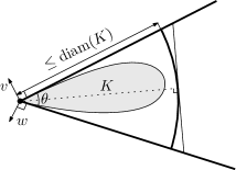
Figure 2. Bound on the volume of a convex set $K$ as a function of the angle between two normal vectors $v,w$ at the same point and its diameter (see Lemma 4.3).

Proof.

The left-hand side of the inequality is non-positive, so the inequality needs only to be proven when $\langle v\mid w\rangle\leqslant 0$, which we assume from now on. Making a rotation of axes and a translation if necessary, we assume that $p$ lies at the orign and that the unit vectors span the first two coordinates of $\mathbb{R}^{d}$. Then, letting $H:=\{p\mid\langle p\mid v\rangle\leqslant 0\}$, $H^{\prime}:=\{p\mid\langle p\mid w\rangle\leqslant 0\}$ and $D$ be the two-dimensional disc centered at $0$ of radius $\operatorname{diam}(K)$, one has

$$K\subseteq H\cap H^{\prime}\cap(D\times[-\operatorname{diam}(K),\operatorname{diam}(K)]^{d-2}).$$

The intersection $H\cap H^{\prime}\cap D$ is an angular sector of the disc $D$, whose angle is equal to $\theta:=\pi-\arccos(\langle v\mid w\rangle)$ (see Figure 2). Therefore, we have

$$\mathcal{H}^{d}(K) \leqslant\mathcal{H}^{d}(H\cap H^{\prime}\cap(D\times[-\operatorname{diam}(K),\operatorname{diam}(K)]^{d-2}))$$

$$\leqslant 2^{d-2}\operatorname{diam}(K)^{d}\tan(\theta/2).$$ (4.21)

Using the expression of $\cos(\theta)$ in term of $\tan(\theta/2)$ and recalling $\langle v\mid w\rangle\leqslant 0$,

$$\tan(\theta/2)=\sqrt{\frac{1+\langle v\mid w\rangle}{1-\langle v\mid w\rangle}}\leqslant\sqrt{1+\langle v\mid w\rangle}$$ (4.22)

The lemma follows directly from Equations (4.21)–(4.22). ∎

Proof of Proposition 4.2.

By definition of the bi-Lipschitz constant $C_{\mathrm{exp}}$,

$$\mathcal{H}^{d}(L_{y}(\psi))\geqslant\varepsilon/(2C_{\mathrm{exp}}^{d}\left\|\rho\right\|_{\infty})\hbox{ and }\operatorname{diam}(L_{y}(\psi))\leqslant C_{\mathrm{exp}}\operatorname{diam}(X).$$

Applying the above lemma to the two outward normals $v,w$ at $p$, we get

$$\langle v\mid w\rangle+1\geqslant\frac{\mathcal{H}^{d}(L_{y}(\psi))^{2}}{4^{d-2}\operatorname{diam}(L_{y}(\psi))^{2d}}\geqslant\frac{\varepsilon^{2}}{4^{d-1}C_{\mathrm{exp}}^{4d}\left\|\rho\right\|_{\infty}^{2}\operatorname{diam}(X)^{2d}}.\qed$$

We also record the following lemma for later use.

Lemma 4.4.

Let $y$ in $Y$ and let $p$ in be a point of $L_{y}(\psi)$ such that for some $z\neq y$,  $f_{z,y}(p)=\psi(z)-\psi(y)$. Then, the point $p^{\prime}:=(\exp_{z}^{c})^{-1}(\exp_{y}^{c}(p))$ belongs to $L_{z}(\psi)$ and the vector $\nabla f_{y,z}(p)$ lies in the normal cone $\mathcal{N}_{p^{\prime}}L_{z}(\psi)$.

Proof.

We introduce the point $x=\exp_{y}^{c}(p)$. The hypothesis is equivalent to $c(x,y)+\psi(y)=c(x,z)+\psi(z).$ Since $p$ belongs to $L_{y}(\psi)$, the point $x$ belongs to $\operatorname{Lag}_{y}(\psi)$. Then, for any $z^{\prime}\in Y$,

$$c(x,z)+\psi(z) =c(x,y)+\psi(y)\leqslant c(x,z^{\prime})+\psi(z^{\prime})$$

thus establishing that $x$ belongs to $\operatorname{Lag}_{z}(\psi)$ or equivalently $p^{\prime}\in L_{z}(\psi)$. ∎

4.2. Upper transversality estimates.

We now turn to the proof of the quantitative transversality estimates. We begin with a bound which involves the condition number of differential of exponential maps, see Remark 4.1. The advantage of this first bound is that we do not have to assume that the points in $Y$ are sampled from a continuous domain. A second transversality estimate is presented in §4.4.

Notation.

We introduce notation that will be used in throughout this section. We fix a point $y_{0}$ in $Y$ and also fix an arbitrary ordering of the remaining points, so that $Y=\{y_{0},y_{1},\ldots,y_{N}\}$. We define $\hat{X}:=X_{y_{0}}$ and for every index $i\in\{1,\ldots,N\}$ we put

$$f_{i}:=f_{y_{i},y_{0}}:p\in\hat{X} \mapsto c(\exp_{y_{0}}^{c}(p),y_{0})-c(\exp_{y_{0}}^{c}(p),y_{i}).$$

By the (Twist) condition, these functions $f_{1},\ldots,f_{N}$ satisfy the non-degeneracy condition (ND), and we have the following inequalities:

$$\varepsilon_{nd}:=\min_{i,j\neq 0}\min_{p\in X_{y_{0}}}\left\|\nabla f_{i}(p)-\nabla f_{j}(p)\right\|\geqslant C_{\mathrm{exp}}^{-1}\varepsilon_{tw}>0,$$ (4.23)

$$\sup_{i\neq 0}\sup_{p\in X_{y_{0}}}\left\|\nabla f_{i}(p)\right\|\leqslant C_{\mathrm{exp}}C_{\nabla}.$$ (4.24)

To any function $\psi:Y\to\mathbb{R}$ we associate the vector

$$\bm{\lambda}_{\psi}: =(\psi(y_{1})-\psi(y_{0}),\ldots,\psi(y_{N})-\psi(y_{0}))\in\mathbb{R}^{N}.$$ (4.25)

We also consider the same family of convex set as in Section 3:

$$K(\bm{\lambda})=\{p\in\hat{X}\mid\forall 1\leqslant i\leqslant N,f_{i}(p)\leqslant\lambda_{i}\},$$

so that $K(\bm{\lambda}_{\psi})=(\exp_{y_{0}}^{c})^{-1}(\operatorname{Lag}_{y_{0}}(\psi))$.

Proposition 4.5.

Assume that $\bm{\lambda}:=\bm{\lambda}_{\psi}$ where $\psi$ belongs to $\mathcal{K}^{\varepsilon/2}$ and let $p$ be a point in $K(\bm{\lambda})$. Then,

Case I:

If $f_{i}(p)=\lambda_{i}$ and $f_{j}(p)=\lambda_{j}$ for $i\neq j$ in $\{1,\ldots,N\}$, then

$$\left(\frac{\langle\nabla f_{i}(p)\mid\nabla f_{j}(p)\rangle}{\left\|\nabla f_{i}(p)\right\|\left\|\nabla f_{j}(p)\right\|}\right)^{2}\leqslant 1-\delta_{1}^{2}.$$ (4.26)

Case II:

If $p\in\partial\hat{X}$ and if $f_{i}(p)=\lambda_{i}$ for some $i$ in $\{1,\ldots,N\}$, then

$$\forall w\in\mathcal{N}_{p}\hat{X},~{}~{}\left(\frac{\langle\nabla f_{i}(p)\mid w\rangle}{\left\|\nabla f_{i}(p)\right\|\left\|w\right\|}\right)^{2}\leqslant 1-\delta_{1}^{2}.$$ (4.27)

In the above inequalities,

$$\delta_{1}:=\frac{\varepsilon_{nd}\delta_{0}}{2C_{\mathrm{exp}}C_{\nabla}C_{\mathrm{cond}}^{2}}.$$

By assumption, all the Laguerre cells associated to $\psi$ contain a mass of at least $\varepsilon/2$. This allows us to apply Proposition 4.2, ensuring that normal vectors cannot be near-opposite, to all the Laguerre cells in their exponential charts. We denote $L_{i}:=L_{y_{i}}(\psi)=(\exp_{y_{i}}^{c})^{-1}(\operatorname{Lag}_{y_{i}}(\psi))$ for brevity.

The proposition also relies on two simple lemmas. The first lemma shows the effect of a diffeomorphism on the normal cone to a convex set, when its image is also convex.

Lemma 4.6.

Let $K\subset\mathbb{R}^{d}$ be a compact, convex set, $F$ be a $\mathcal{C}^{1}$ diffeomorphism from an open neighborhood of $K$ to an open subset of $\mathbb{R}^{d}$, and assume that $F(K)$ is also a convex set. Then, for any point $x$ in $\partial K$ one has

$$\mathcal{N}_{F(x)}(F(K))=[\mathrm{D}F^{-1}_{F(x)}]^{*}(\mathcal{N}_{x}K),$$

where $A^{*}$ denotes the adjoint of $A$.

Proof.

Consider $x$ in $\partial K$, $v\in\mathcal{N}_{x}K$, and define $\varphi(z):=\langle F^{-1}(z)-x\mid v\rangle$. Since $v$ is an outer normal to $K$ at $x$, the restriction of $\varphi$ to the set $F(K)$ is non-positive. Since $F(K)$ is convex, for any point $y\in K$, $F(K)$ contains the segment $[F(x),F(y)]$. We therefore have

$$0 \geqslant\varphi((1-t)F(x)+tF(y))$$

$$\geqslant\varphi(F(x))+t\langle\nabla\varphi(F(x))\mid F(y)-F(x)\rangle-o(t)$$

$$=t\langle[\mathrm{D}F^{-1}_{F(x)}]^{*}(v)\mid F(y)-F(x)\rangle-o(t).$$

where we have used $\varphi(F(x))=0$ and $\nabla\varphi(F(x))=[\mathrm{D}F^{-1}_{F(x)}]^{*}(v)$ to obtain the equality at the end. Dividing by $t$ and taking the limit as $t$ goes to zero, we see that

$$\forall y\in K,~{}~{}\langle[\mathrm{D}F^{-1}_{F(x)}]^{*}(v)\mid F(y)-F(x)\rangle\leqslant 0,$$

thus showing that $[\mathrm{D}F^{-1}_{F(x)}]^{*}(v)$ belongs to the normal cone to $F(K)$ at $F(x)$. The converse inclusion follows from the symmetry of the problem. ∎

The second lemma compares the angle between two vectors and the angle between their image under a linear map, using the generalized Wiedlandt inequality (see [17, Section 3.4]). We identify $\mathbb{R}^{d}$ with its tangent and cotangent spaces through the Euclidean structure. We denote the adjoint of the derivative of the exponential map $\exp^{c}_{y}$ at a point $p$ in $X_{y}$ by

$$(\mathrm{D}\exp^{c}_{y_{i}})^{*}|_{p}:\mathrm{T}^{*}_{\exp^{c}_{y_{i}}(p)}\Omega\to\mathrm{T}^{*}_{p}\mathbb{R}^{d}\cong\mathbb{R}^{d},$$

Lemma 4.7.

Let $y_{k}\neq y_{\ell}\in Y$, let $x$ be a point in $X$ and set $p_{k}:=(\exp_{y_{k}}^{c})^{-1}(x)$ and $p_{\ell}:=(\exp_{y_{\ell}}^{c})^{-1}(x)$ and

$$A=(\mathrm{D}\exp^{c}_{y_{k}}|_{p_{k}})^{*}\circ[(\mathrm{D}\exp^{c}_{y_{l}}|_{p_{l}})^{*}]^{-1}:\mathrm{T}_{p_{\ell}}^{*}\mathbb{R}^{d}\to\mathrm{T}_{p_{k}}^{*}\mathbb{R}^{d}.$$

Then, the following inequalities hold for all $v$, $w$ in $\mathbb{R}^{d}$:

$$C_{\mathrm{cond}}^{-4}\left(1+\frac{\langle v\mid w\rangle}{\left\|v\right\|\left\|w\right\|}\right)\leqslant 1+\frac{\langle Av\mid Aw\rangle}{\left\|Av\right\|\left\|Aw\right\|}\leqslant C_{\mathrm{cond}}^{4}\left(1+\frac{\langle v\mid w\rangle}{\left\|v\right\|\left\|w\right\|}\right).$$

Proof.

Indeed, let $\theta$ be the angle between $v$ and $w$ and $\theta^{\prime}$ be the angle between $Av$ and $Aw$, both in the interval $(0,\pi)$. Let $t:=\tan(\theta/2)$, $t^{\prime}:=\tan(\theta^{\prime}/2)$. The generalized Wiedlandt inequality in [17, Section 3.4] asserts $(1/\operatorname{cond}(A))t\leqslant t^{\prime}\leqslant\operatorname{cond}(A)t$. Expressing $\cos(\theta)$ in term of $t=\tan(\theta/2)$,

$$1+\cos(\theta^{\prime})=1+\frac{1-t^{\prime 2}}{1+t^{\prime 2}}=\frac{2}{1+t^{\prime 2}}\leqslant\operatorname{cond}(A)^{2}(1+\cos(\theta))$$

We conclude the second inequality above by using $\operatorname{cond}(A_{2}^{*}[A_{1}^{*}]^{-1})\leqslant\operatorname{cond}(A_{1})\operatorname{cond}(A_{2})$ and the definition of the constant $C_{\mathrm{cond}}$. For the first inequality, simply note that $\operatorname{cond}(A^{-1})=\operatorname{cond}(A)$. ∎

Proof of Proposition 4.5, case I.

We let

$$V: =\nabla f_{i}(p)=\nabla f_{y_{i},y_{0}}(p),$$

$$W: =\nabla f_{j}(p)=\nabla f_{y_{j},y_{0}}(p),$$

$$v: =\frac{V}{\left\|V\right\|},\quad w:=\frac{W}{\left\|W\right\|}.$$

Switching the indices $i$ and $j$ if necessary, we assume that $\left\|V\right\|\leqslant\left\|W\right\|$. The proof depends on the sign of $\langle W-V\mid V\rangle$ (see Remark 4.3 below for the significance of the sign of this expression). Assume first $\langle W-V\mid V\rangle\leqslant 0$, and let $\alpha_{v}:=1/\left\|V\right\|,\alpha_{w}:=1/\left\|W\right\|$. Then,

$$1-\langle v\mid w\rangle =\frac{1}{2}\left\|v-w\right\|^{2}=\frac{1}{2}\left\|\alpha_{w}(W-V)-(\alpha_{v}-\alpha_{w})V\right\|^{2}$$

$$=\frac{1}{2}\alpha_{w}^{2}\left\|W-V\right\|^{2}+\frac{1}{2}(\alpha_{v}-\alpha_{w})^{2}\left\|V\right\|^{2}-\alpha_{w}(\alpha_{v}-\alpha_{w})\langle W-V\mid V\rangle$$

Using $\alpha_{w}\leqslant\alpha_{v}$, and $\left\|W-V\right\|\geqslant\varepsilon_{nd}$ we end up with

$$1-\langle v\mid w\rangle^{2} \geqslant 1-\langle v\mid w\rangle\geqslant\frac{1}{2}\alpha_{w}^{2}\left\|W-V\right\|^{2}$$

$$\geqslant\frac{1}{2}\frac{\varepsilon_{nd}^{2}}{C_{\mathrm{exp}}^{2}C_{\nabla}^{2}}\geqslant\frac{\varepsilon_{nd}^{2}\delta_{0}^{2}}{4C_{\mathrm{exp}}^{2}C_{\nabla}^{2}C_{\mathrm{cond}}^{4}}=\delta_{1}^{2}$$

where we have used (4.23) and (4.24), $\delta_{0}\leqslant 1$ and $C_{\mathrm{cond}}\geqslant 1$. This establishes the desired bound when $\langle v\mid w\rangle\in[0,1]$. In the case $\langle v\mid w\rangle\in[-1,0]$, we can apply Proposition 4.2 to show that $1-\langle v\mid w\rangle^{2}\geqslant 1+\langle v\mid w\rangle\geqslant\delta_{0}^{2}\geqslant\delta_{1}^{2},$ thus establishing the desired bound.

Now suppose $\langle W-V\mid V\rangle\geqslant 0$. A slightly tedious computation gives

$$\langle v\mid w\rangle^{2} =1-\frac{\left\|W-V\right\|^{2}}{\left\|W\right\|^{2}}+\frac{\langle W-V\mid v\rangle^{2}}{\left\|W\right\|^{2}}$$

$$=1-\frac{\left\|W-V\right\|^{2}}{\left\|W\right\|^{2}}\left(1-\frac{\langle W-V\mid v\rangle^{2}}{\left\|W-V\right\|^{2}}\right)$$

$$\leqslant 1-\frac{\varepsilon_{nd}^{2}}{C_{\mathrm{exp}}^{2}C_{\nabla}^{2}}\left(1-\langle\frac{W-V}{\left\|W-V\right\|}\mid v\rangle\right),$$ (4.28)

where we have used $\langle W-V\mid V\rangle\geqslant 0$ with (4.23) and (4.24) to get the last inequality. We will now apply Proposition 4.2 to the Laguerre cell $L_{i}$. By Lemma 4.4, the point $p_{i}:=(\exp_{y_{i}}^{c})^{-1}(\exp_{y_{0}}^{c}(p))\in X_{y_{i}}$ belong to $L_{i}$ and the vectors $V_{i}:=\nabla f_{y_{0},y_{i}}(p_{i})$ and $W_{i}:=\nabla f_{y_{j},y_{i}}(p_{i})$ are both normals to $L_{i}$ at $p_{i}$. Proposition 4.2 then shows that the vectors $V_{i}$ and $W_{i}$ satisfy

$$-1+\delta_{0}^{2}\leqslant\frac{\langle V_{i}\mid W_{i}\rangle}{\left\|V_{i}\right\|\left\|W_{i}\right\|}.$$ (4.29)

We transfer this inequality to the exponential chart of the original point $y_{0}$ using the linear map

$$A:=(\left.\mathrm{D}\exp_{y_{0}}^{c}\right|_{p})^{*}\circ[(\left.\mathrm{D}\exp_{y_{i}}^{c}\right|_{p_{i}})^{*}]^{-1}.$$

First, note that $W-V=AW_{i}$ and $V=-AV_{i}.$ Applying the generalized Wiedlandt inequality (Lemma 4.7) and (4.29) we have

$$1-\frac{\langle W-V\mid v\rangle}{\left\|W-V\right\|}=1+\frac{\langle AW_{i}\mid AV_{i}\rangle}{\left\|AW_{i}\right\|{\left\|AV_{i}\right\|}} \geqslant C_{\mathrm{cond}}^{-4}\left(1+\frac{\langle V_{i}\mid W_{i}\rangle}{\left\|V_{i}\right\|\left\|W_{i}\right\|}\right)$$

$$\geqslant C_{\mathrm{cond}}^{-4}\delta_{0}^{2}\geqslant\delta_{1}^{2}.$$ (4.30)

Combining this inequality with (4.28) we obtain (4.26) in this case as well. ∎

Proof of Proposition 4.5, case II.

Consider $V:=\nabla f_{i}(p)$ and let $W$ be any vector in the normal cone $\mathcal{N}_{p}\hat{X}$. When $\langle V\mid W\rangle\leqslant 0$, the inequality directly follows from Proposition 4.2, ensuring that normal vectors cannot be near-opposite. We now assume $\langle V\mid W\rangle\geqslant 0$ and we will apply Proposition 4.2 to the Laguerre cell of $y_{i}$ and transfer the result to the exponential chart of the point $y_{0}$. Let $p_{i}=(\exp_{y_{i}}^{c})^{-1}(\exp_{y}^{c}(p))$. Then, by Lemma 4.4, $p_{i}$ belongs to $L_{i}$ and $V_{i}:=\nabla f_{y_{0},y_{i}}(p_{i})$ is a normal vector to $L_{i}$ at $p_{i}$. We define a second normal vector by considering

$$A:=(\left.\mathrm{D}\exp_{y_{0}}^{c}\right|_{p_{0}})^{*}\circ[(\left.\mathrm{D}\exp_{y_{i}}^{c}\right|_{p_{i}})^{*}]^{-1}$$

and by setting $W_{i}:=A^{-1}W\in\mathrm{T}^{*}_{p_{i}}\mathbb{R}^{d}$. By Lemma 4.6, the vector $W_{i}$ belongs to the normal cone to $X_{y_{i}}$ at $p_{i}$. Moreover, since $L_{i}$ is contained in $X_{y_{i}}$ and both sets contain $p_{i}$, we have $\mathcal{N}_{p_{i}}X_{y_{i}}\subseteq\mathcal{N}_{p_{i}}L_{i}$, thus ensuring that $W_{i}$ also belongs to the normal cone to $L_{i}$ at $p_{i}$. Then, by Proposition 4.2 again,

$$\frac{\langle V_{i}\mid W_{i}\rangle}{\left\|V_{i}\right\|\left\|W_{i}\right\|}\geqslant-1+\delta_{0}^{2}.$$

As before, we transfer this inequality to the exponential chart of the original point $y$ using the linear map $A$. We have $V=\nabla f_{i}(p)=-AV_{i}$, and by construction $W=AW_{i}$. We get the desired inequality by applying Lemma 4.7:

$$1-\frac{\langle V\mid W\rangle}{\left\|V\right\|\left\|W\right\|}=1+\frac{\langle AV_{i}\mid AW_{i}\rangle}{\left\|AV_{i}\right\|\left\|AW_{i}\right\|} \geqslant C_{\mathrm{cond}}^{-4}\left(1+\frac{\langle V_{i}\mid W_{i}\rangle}{\left\|V_{i}\right\|\left\|W_{i}\right\|}\right)$$

$$\geqslant C_{\mathrm{cond}}^{-4}\delta_{0}^{2}\geqslant\delta_{1}^{2},$$

and by recalling that $\langle V\mid W\rangle\geqslant 0$. ∎

4.3. Proof of Theorem 4.1

By Theorem 1.1, the second-differentiability of Kantorovich’s functional $\Phi$ will follow from the differentiability of the function

$$G_{y_{0}}(\psi):=\int_{\operatorname{Lag}_{y_{0}}(\psi)}\rho(x)\mathrm{d}\mathcal{H}^{d}_{g}(x)=\int_{L_{y}(\psi)}\hat{\rho}(p)\mathrm{d}p$$

where we have used the change-of-variable formula with $x=\exp_{y_{0}}^{c}(p)$, so that $\hat{\rho}$ is the density of the pushforward measure $(\exp^{c}_{y_{0}})^{-1}_{\#}(\rho\mathcal{H}^{d}_{g})$ with respect to the Lebesgue measure. We recall that

$$K(\bm{\lambda}_{\psi})=(\exp_{y_{0}}^{c})^{-1}(\operatorname{Lag}_{y_{0}}(\psi)),$$

so that $G_{y_{0}}(\psi)=\hat{G}(\bm{\lambda}_{\psi})$ (as defined in (3.12)). The differentiability of $\hat{G}$ will be proven using Theorem 3.1 from the previous section.

Let us fix a function $\psi_{0}$ in $\mathcal{K}^{\varepsilon}$ and recall that $\bm{\lambda}_{0}:=\bm{\lambda}_{\psi_{0}}$. By Proposition 2.3 there exists a positive constant $T_{tr}$ such that every function $\psi$ on $Y$ satisfying $\left\|\psi-\psi_{0}\right\|_{\infty}\leqslant T_{tr}$ belongs to $\mathcal{K}^{\varepsilon/2}$. Then, by Proposition 4.5, we see that the functions $f_{i}$ satisfy the transversality condition (T) on the cube $\bm{\lambda_{0}}+[-T_{tr},T_{tr}]^{N}$ with constant

$$\varepsilon_{tr}=\delta_{1}=\frac{\varepsilon_{nd}\delta_{0}}{2C_{\mathrm{exp}}C_{\nabla}C_{\mathrm{cond}}^{2}},$$ (4.31)

where we recall that $\delta_{0}=\varepsilon/(2^{d}\left\|\rho\right\|_{\infty}{C_{\mathrm{exp}}}^{2d}\operatorname{diam}{(X)}^{d})$. Note also that since $\rho$ is $\alpha$-Hölder and since the exponential map is $\mathcal{C}^{1,1}$, the probability density $\hat{\rho}$ is also $\alpha$-Hölder with constant

$$\left\|\hat{\rho}\right\|_{\mathcal{C}^{0,\alpha}(\hat{X})}\leqslant C(\left\|\rho\right\|_{\mathcal{C}^{0,\alpha}},C_{\mathrm{det}}).$$ (4.32)

We can now apply Theorem 3.1. This ensures that the function $\hat{G}$ is of class $\mathcal{C}^{1,\alpha}$ on the cube $\bm{\lambda_{0}}+[-T_{tr},T_{tr}]^{N}$, so that $\partial\Phi/\partial\mathbbold{1}_{y_{0}}$ is $\mathcal{C}^{1,\alpha}$ on a neighborhood of $\psi_{0}$. Since this holds for any point $y_{0}\in Y$ and any function $\psi_{0}$ in $\mathcal{K}^{\varepsilon}$, we have established the $\mathcal{C}^{2,\alpha}$-regularity of $\Phi$ on $\mathcal{K}^{\varepsilon}$. The claimed dependency of $\left\|\Phi\right\|_{\mathcal{C}^{2,\alpha}(\mathcal{K}^{\varepsilon})}$ follows from equations (4.31)–(4.32) and from Theorem 3.1.

Our goal is now to deduce the formula for the gradient of $G$ given in Theorem 4.1 (Equation (1.8)), from the formula for the gradient of $\hat{G}$ given in Theorem 3.1 (Equation (3.14)). This is done by looking more closely at the change of variable induced by the exponential map $F:=\exp^{c}_{y_{0}}:\Omega\to\mathbb{R}^{d}$. For ease of notation we let $h:=c(\cdot,y_{0})-c(\cdot,y_{i})\lambda=f_{i}\circ F^{-1}$. By definition of the push-forward, we have for any bounded measurable function $\chi$ on $\Omega$,

$$\int_{\hat{\Omega}}\chi(F(p))\rho(p)\mathrm{d}\mathcal{H}^{d}(p)=\int_{\Omega}\chi(x)\hat{\rho}(x)\mathrm{d}\mathcal{H}^{d}_{g}(x).$$

Multiplying $\chi$ by the characteristic function of $h^{-1}([t,s])$, this gives

$$\int_{f_{i}^{-1}([t,s])}\chi(F(p))\hat{\rho}(p)\mathrm{d}\mathcal{H}^{d}(p)=\int_{h^{-1}([t,s])}\chi(x)\rho(x)\mathrm{d}\mathcal{H}^{d}_{g}(x).$$

Applying the coarea formula on both sides, we get

$$\int_{t}^{s}\int_{f_{i}^{-1}(r)}\frac{\chi(F(p))\hat{\rho}(p)}{\left\|\nabla f_{i}(p)\right\|}\mathrm{d}\mathcal{H}^{d-1}(p)\mathrm{d}r=\int_{t}^{s}\int_{h^{-1}(r)}\frac{\chi(x)\rho(x)}{\left\|\nabla h(x)\right\|_{g}}\mathrm{d}\mathcal{H}^{d-1}_{g}(x)\mathrm{d}r.$$ (4.33)

Using the $\mathcal{C}^{1,1}$ smoothness of the functions $f_{i}$ and the (Twist) condition, we can see that for any $\chi$ in $\mathcal{C}^{0}_{c}(\Omega)$, the two inner integrals

$$r\mapsto\int_{f_{i}^{-1}(r)}\frac{\chi(F(p))\hat{\rho}(p)}{\left\|\nabla f_{i}(p)\right\|}\mathrm{d}\mathcal{H}^{d-1}(p)\hbox{ and }r\mapsto\int_{h^{-1}(r)}\frac{\chi(x)\rho(x)}{\left\|\nabla h(x)\right\|_{g}}\mathrm{d}\mathcal{H}^{d-1}_{g}(x)$$

depend continuously on $r$. Using the continuity of these functions in $r$, equation (4.33) and the Fundamental Theorem of Calculus, we get that for any function $\chi$ in $\mathcal{C}^{0}_{c}(\Omega)$ and any $r$ in $\mathbb{R}$,

$$\int_{f_{i}^{-1}(r)}\frac{\chi(F(p))\hat{\rho}(p)}{\left\|\nabla f_{i}(p)\right\|}\mathrm{d}\mathcal{H}^{d-1}(p)=\int_{h^{-1}(r)}\frac{\chi(x)\rho(x)}{\left\|\nabla h(x)\right\|_{g}}\mathrm{d}\mathcal{H}^{d-1}_{g}(x).$$

By Tietze’s extension theorem, (Twist) and (Reg), the level set $S:=h^{-1}(r)$ is a $\mathcal{C}^{1,1}$ hypersurface of $\Omega$. Thus every function in $\mathcal{C}^{0}_{c}(S)$ can be extended to a function in $\mathcal{C}^{0}_{c}(\Omega)$. The previous equality therefore holds for any $\chi$ in $\mathcal{C}^{0}_{c}(S)$, and by density, it also holds for any function $\chi$ in $\mathrm{L}^{1}(S)$. Applying this with $\chi$ equal to the indicator function of the interface between the Laguerre cell of $y_{0}$ and the cell of $y_{i}$, we get the desired formula for the partial derivatives:

$$\frac{\partial G_{i}}{\partial\psi_{i}}(\psi)=\frac{\partial\hat{G}}{\partial\lambda_{i}}(\bm{\lambda}_{\psi}) =\int_{L_{y_{0}}(\psi)\cap f_{i}^{-1}(\psi(y_{i})-\psi(y_{0}))}\frac{\hat{\rho}(p)}{\left\|\nabla f_{i}(p)\right\|}\mathrm{d}\mathcal{H}^{d-1}(p)$$

$$=\int_{\operatorname{Lag}_{y_{0}}(\psi)\cap\operatorname{Lag}_{y_{i}}(\psi)}\frac{\rho(x)}{\left\|Dc_{y_{0}}(x)-Dc_{y_{i}}(x)\right\|_{g}}\mathrm{d}\mathcal{H}_{g}^{d-1}(x).$$

4.4. Alternative upper transversality estimates

Finally, we state an alternate upper transversality estimate, under the assumption that the points in $Y$ are sampled from some target domain $\Lambda$, along with some convexity conditions. Specifically, let $\Lambda$ be a bounded, open subset in some Riemannian manifold, with $Y\subset\Lambda$. We then assume that for any $x^{\prime}\in\Omega^{{\rm{cl}}}$, the mapping

$$y \mapsto-D_{x}c(x^{\prime},y)$$

is a diffeomorphism onto its range, and we denote the inverse by $\exp^{c}_{x^{\prime}}$. We will also assume that $(\exp^{c}_{x})^{-1}(\Lambda)$ is convex for all $x\in\Omega$, and finally that the following inequality holds: for any $x$, $x^{\prime}\in\Omega$, $q_{0}$, $q_{1}\in(\exp^{c}_{x^{\prime}})^{-1}(\Lambda)$, and $t\in[0,1]$,

$$-c(x,\exp_{x^{\prime}}^{c}((1-t)q_{0}+tq_{1}))+c(x^{\prime},\exp_{x^{\prime}}^{c}((1-t)q_{0}+tq_{1})))$$

$$\leqslant\max\{-c(x,\exp_{x^{\prime}}^{c}(q_{0}))+c(x^{\prime},\exp_{x^{\prime}}^{c}(q_{0})),-c(x,\exp_{x^{\prime}}^{c}(q_{1}))+c(x^{\prime},\exp_{x^{\prime}}^{c}(q_{1}))\}$$ (4.34)

Note that this last inequality is nothing but quasi-concavity of $c(x^{\prime},\cdot)-c(x,\cdot)$ in the global coordinate chart of $\Lambda$ defined by $\exp_{x^{\prime}}^{c}$. For more on these conditions, see Remark 4.4 below.

Proposition 4.8 can be applied to provide an alternative bound in the transversality condition (T) when the point $p_{0}\in\partial K(\bm{\lambda})$ is in the interior of $X$ (so in particular, when dealing with Laguerre cells that do not intersect $\partial X$). The advantage of this bound is that it does not require knowledge of the condition number $C_{\mathrm{cond}}$.

Recall that we have fixed some point $y_{0}\in Y=\{y_{1},\ldots,y_{N}\}$ and for any index $i\in\{1,\ldots,N\}$ we use the notation,

$$f_{i}(p)=f_{y_{i},y_{0}}(p)=c(\exp^{c}_{y_{0}}{p},y_{0})-c(\exp^{c}_{y_{0}}{p},y_{i}).$$

We also re-define the constants $C_{\nabla}$ and $C_{\mathrm{exp}}$ so that in their definitions, the maximum of $y$ ranges over the domain $\Lambda$ instead of just $Y$.

Proposition 4.8.

Suppose $\left\|\bm{\lambda}\right\|<T_{tr}<\frac{\varepsilon}{8C_{\mathrm{exp}}^{2d-2}\left\|\rho\right\|_{\infty}\mathcal{H}^{d-1}_{g}(\partial X)}$, and $p_{0}\in K(\bm{\lambda})$ with $f_{i}(p_{0})=\lambda_{i}$ and $f_{j}(p_{0})=\lambda_{j}$ for $i\neq j$ in $\{1,\ldots,N\}$. Then we have

$$\left(\frac{\langle\nabla f_{i}(p_{0})\mid\nabla f_{j}(p_{0})\rangle}{\left\|\nabla f_{i}(p_{0})\right\|\left\|\nabla f_{j}(p_{0})\right\|}\right)^{2}\leqslant 1-\delta_{2}^{2}$$ (4.35)

where

$$\delta_{2}:=\frac{\varepsilon\varepsilon_{nd}}{4\sqrt{2}C_{\nabla}^{2}C_{\mathrm{exp}}^{2d+4}\left\|\rho\right\|_{\infty}\left(\mathcal{H}^{d-1}_{g}(\partial X)\right)}.$$

Remark 4.3.

Before embarking on the proof of this “continuous” upper transversality estimate, we compare some key features of its proof with that of the “discrete” upper transversality estimate Proposition 4.5. By considering the case when the two vectors $\nabla f_{i}(p_{0})$ and $\nabla f_{j}(p_{0})$ are collinear, we can see that both proofs rely on the same core idea. In this case, $\nabla f_{i}(p_{0})$ and $\nabla f_{j}(p_{0})$ are outward normal vectors (in coordinates induced by $\exp^{c}_{y_{0}}$, see Remark 4.4) to the sublevel sets $\{-c(\cdot,y_{0})+\psi(y_{0})\leqslant-c(\cdot,y_{i})+\psi(y_{i})\}$ and $\{-c(\cdot,y_{0})+\psi(y_{0})\leqslant-c(\cdot,y_{j})+\psi(y_{j})\}$ respectively, at $p_{0}$ which lies on the intersection of their boundaries. Since these sets are convex in the associated coordinates, this will cause the Laguerre cell associated to $y_{i}$ to be trapped in a lower dimensional set, giving it zero mass which is a contradiction. The difference between the two proofs lies in quantifying this estimate. In the discrete version of the estimate we do one of two things depending on the sign of the inner product $\langle W-V\mid V\rangle$ (see proof of Proposition 4.5). When this inner product is negative, using that $\left\|W\right\|\geqslant\left\|V\right\|$ and the lower bound on $\left\|W-V\right\|$ from the non-degeneracy condition (ND) yields that $W$ must lie outside of a cone of a certain size opening with axis along $V$. In the other case we note $W-V$ and $-V$ are, respectively, outward normal vectors to the sublevel sets $\{-c(\cdot,y_{i})+\psi(y_{i})\leqslant-c(\cdot,y_{j})+\psi(y_{j})\}$ and $\{-c(\cdot,y_{i})+\psi(y_{i})\leqslant-c(\cdot,y_{0})+\psi(y_{0})\}$, viewed in coordinates given by $\exp_{y_{i}}^{c}$. Thus the lower transversality estimate Proposition 4.2 can be applied to obtain a quantitative bound, but at the price of involving the condition number since we have made a change of coordinates. In the continuous version, there is no change of coordinates, instead we make a rotation to align $\nabla f_{j}(p_{0})$ and $\nabla f_{i}(p_{0})$, then estimate the error induced by this rotation using (4.34), in a vein similar to calculations from [16, Remark 2.5, Proof of Lemma 4.7].

Proof of Proposition 4.8.

Let us again write

$$V: =\nabla f_{i}(p_{0}),\quad W:=\nabla f_{j}(p_{0}),$$

$$v: =\frac{V}{\left\|V\right\|},\quad w:=\frac{W}{\left\|W\right\|},$$

and assume $\varepsilon_{nd}<\left\|V\right\|\leqslant\left\|W\right\|$ and $\langle v\mid w\rangle>0$. Let us also define

$$x_{0}: =\exp^{c}_{y_{0}}(p_{0}),\quad q_{0}:=-D_{x}c(x_{0},y_{0}),\quad q_{1}:=-D_{x}c(x_{0},y_{j}).$$

A quick calculation yields

$$q_{0} =[(\mathrm{D}\exp^{c}_{y_{0}}|_{p_{0}})^{*}]^{-1}(-\nabla_{p}c(\exp^{c}_{y_{0}}(p),y_{0})|_{p=p_{0}}),$$

$$q_{1} =[(\mathrm{D}\exp^{c}_{y_{0}}|_{p_{0}})^{*}]^{-1}(W)+q_{0},$$

Now we define the point

$$q^{\prime}:=[(\mathrm{D}\exp^{c}_{y_{0}}|_{p_{0}})^{*}]^{-1}(\left\|V\right\|w)+q_{0},$$

since $\left\|V\right\|\leqslant\left\|W\right\|$, the above calculation yields that $q^{\prime}$ lies on the line segment between $q_{0}$ and $q_{1}$; since $(\exp^{c}_{x_{0}})^{-1}(\Lambda)$ is convex we have that $q^{\prime}\in(\exp^{c}_{x_{0}})^{-1}(\Lambda)$ as well.

Thus we can define

$$y^{\prime}_{i}: =\exp^{c}_{x_{0}}(q^{\prime}),$$

$$\tilde{f}_{i}(p): =-c(\exp^{c}_{y_{0}}(p),y^{\prime}_{i})+c(\exp^{c}_{y_{0}}(p),y_{0})+c(x_{0},y^{\prime}_{i})-c(x_{0},y_{0})+\lambda_{i},$$

and by (4.34) applied with the choices $x:=\exp^{c}_{y_{0}}(p)$, $x^{\prime}:=x_{0}$, $t:=\frac{\left\|V\right\|}{\left\|W\right\|}$, and $q_{0}$, $q_{1}$ as defined above. we will obtain for all $p\in(\exp^{c}_{y_{0}})^{-1}(\Omega)$,

$$\tilde{f}_{i}(p)-\lambda_{i}\leqslant\max\{0,f_{j}(p)-\lambda_{j}\},$$ (4.36)

while another quick calculation yields

$$y_{i} =\exp^{c}_{x_{0}}([(\left.\mathrm{D}\exp^{c}_{y_{0}}\right|_{p_{0}})^{*}]^{-1}(V)+q_{0}).$$

Now note that

$$\lvert-c(\exp^{c}_{y_{0}}(p),y^{\prime}_{i})+c(\exp^{c}_{y_{0}}(p),y_{i})\rvert$$

$$\leqslant\sup_{(x,q)\in\Omega\times(\exp^{c}_{x_{0}})^{-1}(\Lambda)}\left\|(\left.\mathrm{D}\exp^{c}_{x_{0}}\right|_{q})^{*}(-D_{y}c(x,\exp^{c}_{x_{0}}(q)))\right\|\left\|[(\left.\mathrm{D}\exp^{c}_{y_{0}}\right|_{p_{0}})^{*}]^{-1}(\left\|V\right\|w-V)\right\|$$

$$\leqslant C_{\nabla}C_{\mathrm{exp}}^{2}\left\|\left\|V\right\|w-V\right\|,$$

where we have used that if $y=\exp^{c}_{x_{0}}(q)$, then $(\left.\mathrm{D}\exp^{c}_{x_{0}}\right|_{q})^{*}=\left.\mathrm{D}\exp^{c}_{y}\right|_{-D_{x}c(x_{0},y)}$. As a result we obtain

$$\lvert\tilde{f}_{i}(p)-f_{i}(p)\rvert^{2}=\lvert-c(\exp^{c}_{y_{0}}(p),y^{\prime}_{i})+c(\exp^{c}_{y_{0}}(p),y_{i})\rvert^{2}$$

$$\leqslant(C_{\nabla}C_{\mathrm{exp}}^{2})^{2}\left\|V-\left\|V\right\|w\right\|^{2}=2(C_{\nabla}C_{\mathrm{exp}}^{2})^{2}\left\|V\right\|^{2}(1-\langle v\mid w\rangle)$$

$$\leqslant 2(C_{\nabla}C_{\mathrm{exp}}^{2})^{2}(C_{\mathrm{exp}}C_{\nabla})^{2}(1-\langle v\mid w\rangle).$$

Combining with (4.36) we then have for any $p\in(\exp^{c}_{y_{0}})^{-1}(\Omega)$,

$$f_{i}(p)-\lambda_{i}\leqslant\max\{0,\ f_{j}(p)-\lambda_{j}\}+\sqrt{2}C_{\mathrm{exp}}^{3}C_{\nabla}^{2}\sqrt{1-\langle v\mid w\rangle}$$

or re-arranging and using that $\left\|\bm{\lambda}\right\|<T_{tr}$,

$$1-\langle v\mid w\rangle \geqslant\sup_{p\in(\exp^{c}_{y_{0}})^{-1}(\Omega)}\frac{(f_{i}(p)-\max\{0,f_{j}(p)\}-2T_{tr})^{2}}{2(C_{\mathrm{exp}}^{3}C_{\nabla}^{2})^{2}}.$$ (4.37)

We now make the following observation. Let us write $X_{i}:=(\exp^{c}_{y_{i}})^{-1}(X)$. Then for any $t$, $s>0$, we can estimate the volume of $X_{i}\cap\{f_{y_{0},y_{i}}\leqslant-t\}\cap\{f_{y_{j},y_{i}}\leqslant-s\}$ by

$$\mathcal{H}^{d}\left(X_{i}\cap\{f_{y_{0},y_{i}}\leqslant-t\}\cap\{f_{y_{j},y_{i}}\leqslant-s\}\right)$$

$$\geqslant\mathcal{H}^{d}\left(X_{i}\cap\{f_{y_{0},y_{i}}\leqslant 0\}\cap\{f_{y_{j},y_{i}}\leqslant 0\}\right)-\mathcal{H}^{d}\left(X_{i}\cap\{-t<f_{y_{0},y_{i}}\leqslant 0\}\right)$$

$$\quad-\mathcal{H}^{d}\left(X_{i}\cap\{-s<f_{y_{j},y_{i}}\leqslant 0\}\right).$$

Using that $L_{i}\subset\{f_{y_{0},y_{i}}\leqslant 0\}\cap\{f_{y_{j},y_{i}}\leqslant 0\}$, we can bound the first term from below as

$$\mathcal{H}^{d}\left(X_{i}\cap\{f_{y_{0},y_{i}}\leqslant 0\}\cap\{f_{y_{j},y_{i}}\leqslant 0\}\right)\geqslant\frac{\varepsilon}{C_{\mathrm{exp}}^{d}\left\|\rho\right\|_{\infty}}.$$

For the second term, by the coarea formula, we can write

$$\mathcal{H}^{d}\left(X_{i}\cap\{-t<f_{y_{0},y_{i}}\leqslant 0\}\right) \leqslant\int_{-t}^{0}\int_{X_{i}\cap\{f_{y_{0},y_{i}}=z\}}\frac{1}{\left\|\nabla f_{y_{0},y_{i}}(p)\right\|}d\mathcal{H}^{d-1}(p)dz$$

$$\leqslant\frac{t\mathcal{H}^{d-1}(\partial X_{i})}{\varepsilon_{nd}}\leqslant\frac{tC_{\mathrm{exp}}^{d-1}\mathcal{H}^{d-1}_{g}(\partial X)}{\varepsilon_{nd}},$$

where to obtain the second line we have again used the fact that for every $z\in\mathbb{R}$, the set $X_{i}\cap\{f_{y_{0},y_{i}}=z\}$ is contained in the boundary of a convex subset of $X_{i}$ in conjunction with [21, Remark 5.2]. By a similar bound on the third term, we see that as long as

$$\max\{t,\ s\}<\frac{\varepsilon\varepsilon_{nd}}{2C_{\mathrm{exp}}^{2d-2}\left\|\rho\right\|_{\infty}\mathcal{H}^{d-1}_{g}(\partial X)}$$

we have

$$\mathcal{H}^{d}\left(X_{i}\cap\{f_{y_{0},y_{i}}\leqslant-t\}\cap\{f_{y_{j},y_{i}}\leqslant-s\}\right)>0,$$

thus in particular, (by continuity of $f_{y_{0},y_{i}}$ and $f_{y_{j},y_{i}}$) there must exist a point $p^{\prime}_{c}\in X_{i}$ for which $\max\{f_{y_{0},y_{i}}(p^{\prime}_{c}),\ f_{y_{j},y_{i}}(p^{\prime}_{c})\}\leqslant-\frac{\varepsilon\varepsilon_{nd}}{2C_{\mathrm{exp}}^{2d-2}\left\|\rho\right\|_{\infty}\mathcal{H}^{d-1}_{g}(\partial X)}$. Translating this back into coordinates in $(\exp^{c}_{0})^{-1}(X)$ and in terms of $f_{i}$, $f_{j}$, we see there exists a point $p_{c}\in(\exp^{c}_{0})^{-1}(X)$ for which

$$f_{i}(p_{c})-\max\{0,\ f_{j}(p_{c})\}\geqslant\frac{\varepsilon\varepsilon_{nd}}{2C_{\mathrm{exp}}^{2d-2}\left\|\rho\right\|_{\infty}\mathcal{H}^{d-1}_{g}(\partial X)}.$$

Thus if we have $T_{tr}\leqslant\frac{\varepsilon\varepsilon_{nd}}{8C_{\mathrm{exp}}^{2d-2}\left\|\rho\right\|_{\infty}\mathcal{H}^{d-1}_{g}(\partial X)}$, combining with (4.37) we will obtain the bound (4.35) as desired. ∎

Remark 4.4.

Under a set of standard conditions, we can obtain both (QC) and (4.34).

Let $\Omega$ and $\Lambda$ be bounded and smooth domains in $d$ dimensional Riemannian manifolds and take a cost $c\in C^{4}(\overline{\Omega}\times\overline{\Lambda})$. Also assume

• $c$ satisfies the (Twist) condition: for every $x\in\Omega$, the map $y\in\Lambda\mapsto-D_{x}c(x,y)$ is a diffeomorphism onto its image $\Lambda_{x}:=-D_{x}c(x,\Lambda)\subset T^{*}_{x}\Omega$ and we define the $c$-exponential map $\exp^{c}_{x}:\Lambda_{x}\to\Lambda$ by $\exp^{c}_{x}=(-D_{x}c(x,\cdot))^{-1}$.

• the cost $c^{*}(x,y):=c(y,x)$ satisfies the (Twist) condition: for every $y\in\Lambda$, we can define the $c^{*}$-exponential map $\exp^{c}_{y}:\Omega_{y}\to\Omega$ on the set $\Omega_{y}:=-D_{y}c(\Omega,y)\subset T^{*}_{y}\Lambda$ by $\exp^{c}_{y}=(-D_{y}c(\cdot,y))^{-1}$.

• $(\exp^{c}_{x})^{-1}(\Lambda)$ is convex for each $x\in\Omega$.

• $(\exp^{c^{*}}_{y})^{-1}(\Omega)$ is convex for each $y\in\Lambda$.

• $\det D^{2}_{xy}c(x,y)\neq 0$ for all $(x,y)\in\overline{\Omega}\times\overline{\Lambda}$.

• For any $(x,y)\in\overline{\Omega}\times\overline{\Lambda}$ and $\eta\in T^{*}_{x}\Omega$, $V\in T_{x}\Omega$ with $\eta(V)=0$,

  $$-(c_{ij,pq}-c_{ij,r}c^{r,s}c_{s,pq})c^{p,k}c^{q,l}V^{i}V^{j}\eta_{k}\eta_{l}\geqslant 0,$$ (A3w)

here indices before a comma are derivatives on $\Omega$ and after a comma on $\Lambda$, for fixed coordinate systems, and a pair of raised indices denotes the inverse of a matrix. This last condition (A3w) originates (in a stronger version) in [26] related to regularity of optimal transport. [23, Theorem 3.2] in the Euclidean case and [20, Theorem 4.10] in the general manifold case show the above conditions imply (QC) and (4.34). In fact, they are equivalent as seen in [23]. This geometric interpretation is a key ingredient in showing regularity in the optimal transport problem in the vein of Caffarelli’s classical work [7], see [13, 16].

5. Strong concavity of Kantorovich’s functional

We establish in this section the strong concavity of Kantorovich’s functional $\Phi$ over some suitable domain of $\mathbb{R}^{Y}$. As explained in the introduction, $\Phi$ is invariant under addition of a constant, so that we must restrict ourselves to the orthogonal complement $E_{Y}$ of the space of constant functions. Moreover, we will consider the set $\mathcal{K}^{\varepsilon}$ defined by (4.18), which can be thought of as the space of strictly $c$-concave functions. Recall that the conditions (Reg), (Twist), (QC), and (PW) are defined in the introduction, on pages Reg, Twist, QC, and PW respectively.

Theorem 5.1.

Assume (Reg), (Twist), (QC). Let $X$ be a compact, $c$-convex subset of $\Omega$, and $\rho$ be a continuous probability density on $X$ satisfying (PW). Then, there exists a positive constant $C$, such that

$$\forall\psi\in\mathcal{K}^{\varepsilon},~{}\forall v\in E_{Y},~{}~{}\langle\mathrm{D}^{2}\Phi(\psi)v\mid v\rangle\leqslant-C\cdot\varepsilon^{3}\left\|v\right\|^{2},$$

where $C$ is defined in (5.46), and depends on $\left\|\rho\right\|_{\infty}$, $\mathcal{H}^{d-1}_{g}(\partial X)$, and $C_{\mathrm{exp}}$, $C_{\nabla}$, and $\varepsilon_{tw}$ from Remark 4.1.

Remark 5.1.

Note that the upper bound on the largest non-zero eigenvalue of $\mathrm{D}^{2}\Phi(\psi)$ degrades as $N$ grows to infinity, since $\varepsilon$ is of the order of $1/N$. A possible place for improvement is the reverse isoperimetric inequality stated in equation (5.43). Currently, we are vastly overestimating the size of the boundary of a Laguerre cell by bounding it with the area of the boundary of the whole domain, additionally we are bounding the density $\rho$ by its supremum, and paying in terms of the constant $C_{\mathrm{exp}}$. Note that (5.43) in its current form can never achieve equality, even for constant density $\rho$ and the quadratic cost function where $C_{\mathrm{exp}}=1$, as equality would only happen for a Laguerre cell that occupied the whole domain $X$, which can not happen as all Laguerre cells have nonzero mass. To improve the inequality, one could try to control the anisotropy of Laguerre cells and bound the area of the boundary of a cell by some fraction of the area of $\partial X$, however this would require assumptions on the distribution of the points $Y$ and on $\nu\in\mathcal{P}(Y)$. We believe that such an upper bound on the anisotropy of Laguerre cells would be interesting in itself, and heuristically seems feasible to view as a discrete analogue of the regularity results for optimal transport (interpreting the Laguerre cells associated to $\psi:Y\to\mathbb{R}$ as the $c^{*}$-subdifferentials of $\psi$).

Remark 5.2.

Note that unlike the domain $X$, the support of the density $\rho$ does not need be $c$-convex. We provide in Appendix A an example of a radial measure on $\mathbb{R}^{d}$ whose support is an annulus (hence is not simply connected) but whose Poincaré-Wirtinger constant (PW) is nonetheless positive.

The end of the section is devoted to the proof of Theorem 5.1. It relies on the fact that $-\mathrm{D}^{2}\Phi(\psi)$ can be regarded as the Laplacian matrix of a weighted graph on $Y$, whose first nonzero eigenvalue can be controlled from below using the Cheeger constant of the weighted graph. In turn, this weighted Cheeger constant can be controlled using the Poincaré-Wirtinger inequality.

5.1. Poincaré inequality and continuous Cheeger constant

We start by proving that the finiteness of the Poincaré-Wirtinger constant of the weighted domain $(X,\rho)$ implies the positivity of the weighted Cheeger constant, defined in (5.38). In the following, a Lipschitz domain denotes the closure of an open set with Lipschitz boundary.

Lemma 5.2.

Assume (QC) and that $X$ is compact and $c$-convex. Then

• $X$ is a Lipschitz domain,

• for any $\psi\in\mathcal{K}^{+}$ and $y$ in $Y$, $\operatorname{Lag}_{y}(\psi)\cap X$ is a Lipschitz domain.

Proof.

By assumption, for any $y\in Y$ one can write $X=\exp_{y}^{c}(X_{y})$ where $X_{y}$ is a bounded convex subset of $\mathbb{R}^{d}$ which must have nonempty interior since it supports an absolutely continuous probability measure. Moreover, the map $\exp_{y}^{c}$ is a diffeomorphism, hence bi-Lipschitz. This implies (i), while (ii) follows from the exact same arguments, remembering that $\rho(\operatorname{Lag}_{y}(\psi))>0$. ∎

Given a Lipschitz domain $A$ of $X$ we write, slightly abusing notations,

$$\left|\partial A\right|_{\rho}:=\int_{\partial A\cap\mathrm{int}(X)}\rho(x)\mathrm{d}\mathcal{H}^{d-1}_{g}(x)~{}\hbox{ and }~{}\left|A\right|_{\rho}:=\int_{A}\rho(x)\mathrm{d}\mathcal{H}^{d}_{g}(x).$$

Lemma 5.3.

Let $X$ be a compact domain of $\Omega$ and $\rho$ in $\mathcal{C}^{0}(X)$ be a probability density with finite Poincaré-Wirtinger constant (PW). Then the weighted Cheeger constant of $(X,\rho)$ is positive, that is

$$\mathrm{h}(\rho):=\inf_{A\subseteq X}\frac{\left|\partial A\right|_{\rho}}{\min(\left|A\right|_{\rho},\left|X\setminus A\right|_{\rho})}\geqslant\frac{2}{C_{\mathrm{pw}}},$$ (5.38)

where the infimum is taken over Lipschitz domains $A\subseteq\mathrm{int}(X)$ whose boundary has finite $\mathcal{H}^{d-1}_{g}$–measure.

The proof is based on properties of functions with bounded variation. For more details on this topic, we refer the reader to [4]. Although the discussion in the reference is on Euclidean spaces, the relevant results easily extend to the Riemannian case, as $\exp^{c}_{y}$ serves as a global coordinate system on all of $\Omega$.

Proof.

Let $A$ be a Lipschitz domain $A$ of $\mathrm{int}(X)$. Since $A$ has a Lipschitz boundary with finite area, its indicator function $\chi_{A}$ has bounded variation in $\mathrm{int}(X)$. By the density theorem [4, Theorem 10.1.2], there exists a sequence of $\mathcal{C}^{1}$-functions $f_{n}$ on $\mathrm{int}(X)$ that converges to $\chi_{A}$ in the sense of intermediate convergence (whose definition is not important here). By (PW),

$$\left\|f_{n}-\mathbb{E}_{\rho}(f_{n})\right\|_{L^{1}(\rho)}\leqslant C_{\mathrm{pw}}\ \left\|\nabla f_{n}\right\|_{L^{1}(\rho)}.$$

Since intermediate convergence is stronger than $L^{1}$ convergence, the continuity of $\rho$ implies

$$\lim_{n\to\infty}\left\|f_{n}-\mathbb{E}_{\rho}(f_{n})\right\|_{L^{1}(\rho)}=\left\|\chi_{A}-\mathbb{E}_{\rho}(\chi_{A})\right\|_{L^{1}(\rho)}=2\left|A\right|_{\rho}\ \left|X\setminus A\right|_{\rho}.$$

Note that we used the fact that $\rho$ is a probability measure, i.e. $\rho(X)=1$. Proposition 10.1.2 of [4] implies that the total variation measure $|Df_{n}|$ narrowly converges to $|D\chi_{A}|$, which with the continuity of $\rho$ implies that $\int_{\Omega}|Df_{n}|\rho\mathrm{d}\mathcal{H}^{d}_{g}$ converges to $\int_{\Omega}|D\chi_{A}|\rho\mathrm{d}\mathcal{H}^{d}_{g}=\left|\partial A\right|_{\rho}$. The relation $|Df_{n}|=\left\|\nabla f_{n}\right\|_{g}\mathrm{d}\mathcal{H}^{d}_{g}$ then gives

$$\lim_{n\to\infty}\left\|\nabla f_{n}\right\|_{L^{1}(\rho)}\leqslant\left|\partial A\right|_{\rho}.$$

Combining the previous equations together leads to the desired inequality. ∎

5.2. Cheeger constant of a graph

The goal of this section is to give a lower bound of the second eigenvalue of $-\mathrm{D}^{2}\Phi(\psi)$ in terms of the Cheeger constant of the weighted graph induced by this matrix. An unoriented weighted graph can always be represented by its adjacency matrix $(w_{yz})_{(y,z)\in Y^{2}}$, a symmetric matrix with zero diagonal entries. We introduce a few definitions from graph theory, following the conventions of [14].

Definition 5.1.

Let $(w_{yz})_{(y,z)\in Y^{2}}$ be a weighted graph over $Y$. The (weighted) degree of a vertex $y$ is $d_{y}:=\sum_{z\neq y}w_{yz}$. The (weighted) Laplacian is the matrix $(L_{yz})_{(y,z)\in Y^{2}}$ whose entries are $L_{yz}=-w_{yz}$ for $y\neq z$ and $L_{yy}=d_{y}$.

Definition 5.2.

The Cheeger constant of a weighted graph $(w_{yz})_{(y,z)\in Y^{2}}$ over a point set $Y$ is given by

$$\mathrm{h}(w):=\min_{S\subseteq Y}\frac{\left|\partial S\right|_{w}}{\min(\left|S\right|_{w},\left|Y\setminus S\right|_{w})},$$

$$\hbox{where }\left|\partial S\right|_{w}:=\sum_{y\in S,z\not\in S}w_{yz}\quad\hbox{ and }\quad\left|S\right|_{w}:=\sum_{y\in S}d_{y}.$$

The (weighted) Cheeger inequality bounds from below the first nonzero eigenvalue of the Laplacian of a weighted graph, denoted $\lambda(w)$, from its Cheeger constant and its minimal degree. The formulation we use can be deduced from Corollary 2.2 of [14] and from the inequality $1-\sqrt{1-x^{2}}\geqslant x^{2}/2.$

Theorem 5.4 (Cheeger inequality).

$\lambda(w)\geqslant\frac{1}{2}\ \mathrm{h}^{2}(w)\cdot\min_{y\in Y}d_{y}.$

We now proceed to the proof of the main theorem of this section.

5.3. Proof of Theorem 5.1

Let $\psi$ be a function in $\mathcal{K}^{\varepsilon}$ and consider the weighted graph $(w_{yz})_{(y,z)\in Y^{2}}$ given by

$$w_{yz}:=-\frac{\partial^{2}\Phi}{\partial\mathbbold{1}_{y}\partial\mathbbold{1}_{z}}(\psi)=\int_{\operatorname{Lag}_{y,z}(\psi)}\frac{\rho(x)}{\left\|D_{x}c(x,y)-D_{x}c(x,z)\right\|_{g}}\mathrm{d}\mathcal{H}^{d-1}_{g}(x)$$

for $y\neq z$ in $Y$, and with zero diagonal entries ($w_{yy}=0$). In the formula above, we used the notation $\operatorname{Lag}_{y,z}(\psi)=\operatorname{Lag}_{y}(\psi)\cap\operatorname{Lag}_{z}(\psi)$ for the facet between two Laguerre cells. By construction, the Laplacian matrix of this weighted graph is the Hessian matrix $-\mathrm{D}^{2}\Phi(\psi)$, so that Theorem 5.4 directly gives us a lower bound on the first nonzero eigenvalue of $-\mathrm{D}^{2}\Phi(\psi)$. To complete the proof, we need to bound the Cheeger constant and the minimum degree of the graph $w$ from below.

Step 1

The goal here is to bound from below the discrete Cheeger constant $\mathrm{h}(w)$ in terms of the continuous weighted Cheeger constant $\mathrm{h}(\rho)$ and the constants introduced in (4.19). By definition of the constants $\varepsilon_{tw}$ and $C_{\nabla}$, for every $y\neq z$ in $Y$, one has

$$\varepsilon_{tw}\ w_{yz}\leqslant|\operatorname{Lag}_{y,z}(\psi)|_{\rho}\leqslant 2C_{\nabla}w_{yz}.$$ (5.39)

Consider a subset $S$ of $Y$, and let $A=\cup_{y\in S}\operatorname{Lag}_{y}(\psi)$. Then, the intersection of the boundary of $A$ with $X$ is contained an union of facets of Laguerre cells, namely

$$\partial A\cap\mathrm{int}(X)\subseteq\bigcup_{y\in S,z\not\in S}\operatorname{Lag}_{y,z}(\psi).$$ (5.40)

The two inequalities (5.39) and (5.40) imply a lower bound on the numerator of the Cheeger constant:

$$\left|\partial A\right|_{\rho}\leqslant\sum_{y\in S,z\not\in S}\left|\operatorname{Lag}_{y,z}(\psi)\right|_{\rho}\leqslant 2C_{\nabla}\,\left|\partial S\right|_{w}.$$ (5.41)

We now need to bound the denominator of the Cheeger constant from above, which requires us to control the weighted degrees $\mathrm{d}_{y}$. Note that

$$\mathrm{d}_{y}=\sum_{z\neq y}w_{yz}\leqslant\frac{1}{\varepsilon_{tw}}\sum_{z\neq y}|\operatorname{Lag}_{y,z}(\psi)|_{\rho}\leqslant\frac{1}{\varepsilon_{tw}}|\partial\operatorname{Lag}_{y}(\psi)|_{\rho},$$ (5.42)

where the second inequality comes from the fact that the facets $\operatorname{Lag}_{y,z}(\psi)$ form a partition of the boundary $\partial\operatorname{Lag}_{y}(\psi)\cap\mathrm{int}(X)$ up to a $\mathcal{H}^{d-1}_{g}$–negligible set. To see that this is the case, it suffices to remark that in the exponential chart of $y$, the intersection of two distinct facets adjacent to $y$ has a finite $\mathcal{H}^{d-2}_{g}$–measure, as implied by Proposition 3.2.

In order to apply the (continuous) Cheeger inequality, we need to replace the weighted area of the boundaries of Laguerre cells in (5.42) by the weighted volume of the cells. We have

$$\mathcal{H}^{d-1}_{g}(\partial\operatorname{Lag}_{y}(\psi)) \leqslant C_{\mathrm{exp}}^{d-1}\mathcal{H}^{d-1}((\exp_{y}^{c})^{-1}\partial\operatorname{Lag}_{y}(\psi))$$

$$\leqslant C_{\mathrm{exp}}^{d-1}\mathcal{H}^{d-1}(\partial X_{y})$$

$$\leqslant C_{\mathrm{exp}}^{2(d-1)}\mathcal{H}^{d-1}_{g}(\partial X).$$

The first and third inequalities use the definition of the bi-Lipschitz constant $C_{\mathrm{exp}}$ of the exponential map, while the second inequality uses the monotonicity of the $\mathcal{H}^{d-1}$–measure of the boundary of a convex set with respect to inclusion (see [32, p.211]). Using the assumption $\left|\operatorname{Lag}_{y}(\psi)\right|_{\rho}\geqslant\varepsilon$, this gives us a (rather crude) reverse isoperimetric inequality

$$\left|\partial\operatorname{Lag}_{y}(\psi)\right|_{\rho} \leqslant\left\|\rho\right\|_{\infty}\mathcal{H}^{d-1}_{g}(\partial\operatorname{Lag}_{y}(\psi))$$ (5.43)

$$\leqslant\frac{\left\|\rho\right\|_{\infty}}{\varepsilon}C_{\mathrm{exp}}^{2(d-1)}\mathcal{H}^{d-1}_{g}(\partial X)\left|\operatorname{Lag}_{y}(\psi)\right|_{\rho}$$

We remark here that the above inequality is never sharp, see also Remark 5.1. Combining (5.42), (5.43) and $\left|A\right|_{\rho}=\sum_{y\in S}\left|\operatorname{Lag}_{y}(\psi)\right|_{\rho}$ we obtain

$$\left|S\right|_{w}=\sum_{y\in S}\mathrm{d}_{y}\leqslant\frac{1}{\varepsilon}\frac{\left\|\rho\right\|_{\infty}C_{\mathrm{exp}}^{2(d-1)}\mathcal{H}^{d-1}_{g}(\partial X)}{\varepsilon_{tw}}\left|A\right|_{\rho}.$$

The same inequality holds for the complement $\left|X\setminus S\right|$. We combine the previous inequality with Equation (5.41) and with Lemma 5.3 to get a lower bound on the Cheeger constant

$$\mathrm{h}(w)\geqslant\frac{\varepsilon_{tw}\varepsilon}{C_{\mathrm{exp}}^{2(d-1)}C_{\nabla}\mathcal{H}^{d-1}_{g}(\partial X)\left\|\rho\right\|_{\infty}C_{\mathrm{pw}}}.$$ (5.44)

Note that, in order to apply Lemma 5.3 we implicitly used the fact that $A$ is a Lipschitz domain (as a finite union of Lipschitz domains, see Lemma 5.2) whose boundary has finite $\mathcal{H}^{d-1}_{g}$–measure (by Equation (5.43)).

Step 2

In order to apply the Cheeger inequality, we still need to bound from below the weighted degree $d_{y}$. By (5.39) one has, using the crucial fact that $\left|\partial\operatorname{Lag}_{y}(\psi)\right|_{\rho}$ is the measure of $\partial\operatorname{Lag}_{y}(\psi)\cap\mathrm{int}(X)$,

$$d_{y}=\sum_{z\neq y}w_{yz}\geqslant\frac{1}{2C_{\nabla}}\sum_{z\neq y}\left|\operatorname{Lag}_{y,z}(\psi)\right|_{\rho}\geqslant\frac{1}{2C_{\nabla}}\left|\partial\operatorname{Lag}_{y}(\psi)\right|_{\rho}.$$

Taking $A=\operatorname{Lag}_{y}(\psi)$ in the definition of the weighted Cheeger constant $\mathrm{h}(\rho)$ defined in Lemma 5.3, one gets

$$\left|\partial\operatorname{Lag}_{y}(\psi)\right|_{\rho}\geqslant\mathrm{h}(\rho)\ \min(\left|\operatorname{Lag}_{y}(\psi)\right|_{\rho},\left|X\setminus\operatorname{Lag}_{y}(\psi)\right|_{\rho})\geqslant\mathrm{h}(\rho)\varepsilon.$$

The last inequality comes from the assumption that each Laguerre cell has a mass greater than $\varepsilon$ and that $X\setminus\operatorname{Lag}_{y}(\psi)$ also contains a Laguerre cell (except for the trivial case where $Y$ is a singleton). We deduce

$$d_{y}\geqslant\frac{\varepsilon}{C_{\nabla}C_{\mathrm{pw}}}.$$ (5.45)

Step 3

Combining the Cheeger inequality with Equation (5.44) and (5.45) we have $\lambda(w)\geqslant C\varepsilon^{3}$ where

$$C:=\frac{\varepsilon_{tw}^{2}}{2C_{\mathrm{exp}}^{4(d-1)}C_{\nabla}^{3}\left(\mathcal{H}^{d-1}_{g}(\partial X)\right)^{2}\left\|\rho\right\|^{2}_{\infty}C_{\mathrm{pw}}^{3}}.$$ (5.46)

Since the graph induced by the Hessian is connected, the kernel of $-\mathrm{D}^{2}\Phi(\psi)$ is equal to the space of constant functions over $Y$, implying that $\operatorname{Ker}(-\mathrm{D}^{2}\Phi(\psi))^{\perp}=E_{Y}$. Then, using the variational characterization of the first nonzero eigenvalue of the Laplacian matrix we get:

$$C\varepsilon^{3}\leqslant\lambda(w)=\min_{v\in E_{Y}}\frac{\langle-D^{2}\Phi(\psi)\mid v\rangle}{\left\|v\right\|^{2}}.$$ ∎

6. Convergence of the damped Newton algorithm

The goal of this section is to show the convergence of the Damped Newton algorithm for semi-discrete optimal transport. This follows in fact from a more general result. We establish in Section 6.1 the convergence of the damped Newton algorithm (Algorithm 1) under general assumptions on the functional. We finally apply this algorithm to the semi-discrete optimal transport problem, using the intermediate results (regularity and strict concavity of the Kantorovich functional) proven in Section 4 and 5.

6.1. General damped Newton algorithm

Let $Y$ be a finite set and denote $\mathbb{R}^{Y}$ the space of functions on $Y$. We consider $\mathcal{P}(Y)$, the space of probability measures on $Y$, as a subset of $\mathbb{R}^{Y}$. Finally, we denote by $E_{Y}$ the space of functions on $Y$ who sum to zero. In this section, we show that Algorithm 1 can be used to solve non-linear equations $G(\psi)=\mu$ where $\mu\in\mathcal{P}(Y)$ and the map $G:\mathbb{R}^{Y}\to\mathcal{P}(Y)$ satisfies some regularity and monotonicity assumptions.

Proposition 6.1.

Let $G$ be a functional from $\mathbb{R}^{Y}$ to $\mathcal{P}(Y)$ which is invariant under addition of a constant. Let $G(\psi)=\sum_{y\in Y}G_{y}(\psi)\mathbbold{1}_{y}$ and

$$\mathcal{K}^{\varepsilon}=\{\psi\in\mathbb{R}^{Y}\mid\forall y\in Y,~{}G_{y}(\psi)\geqslant\varepsilon\},$$

and assume that $G$ has the following properties:

• (Regularity) For every positive $\varepsilon$, $G$ is $\mathcal{C}^{1,\alpha}$ on $\mathcal{K}^{\varepsilon}$. We let $L_{\varepsilon}$ be the smallest constant such that

  $$\forall\varphi\neq\psi\in\mathcal{K}^{\varepsilon},~{}~{}\frac{\left\|G(\varphi)-G(\psi)\right\|}{\left\|\varphi-\psi\right\|}+\frac{\left\|\mathrm{D}G(\varphi)-\mathrm{D}G(\psi)\right\|}{\left\|\varphi-\psi\right\|^{\alpha}}\leqslant L_{\varepsilon}.$$

• (Uniform monotonicity) For every $\varepsilon>0$, there exists a positive constant $\kappa_{\varepsilon}$ such that $G$ is $\kappa_{\varepsilon}$–uniformly monotone on $\mathcal{K}^{\varepsilon}\cap E_{Y}$:

  $$\forall\psi\in\mathcal{K}^{\varepsilon},\forall v\in E_{Y},~{}~{}\langle v\mid\mathrm{D}G(\psi)v\rangle\geqslant\kappa_{\varepsilon}\left\|v\right\|^{2}.$$

Now, let $\mu\in\mathcal{P}(Y)$ and let $\psi_{0}$ be a function on $Y$ such that the constant $\varepsilon_{0}$ defined in (1.6) is positive. Set $\kappa:=\min(\kappa_{\frac{1}{2}\varepsilon_{0}},1)$ and $L:=\max(L_{\frac{1}{2}\varepsilon_{0}},1)$. Then, the iterates $(\psi_{k})$ of Algorithm 1 satisfy

$$\left\|G(\psi_{k+1})-\mu\right\|\leqslant(1-\overline{\tau}_{k}/2)\left\|G(\psi_{k})-\mu\right\|$$

$$\hbox{ where }\overline{\tau}_{k}:=\min\left(\frac{\kappa^{1+\frac{1}{\alpha}}\varepsilon}{d^{\frac{1}{\alpha}}L^{\frac{1}{\alpha}}\left\|G(\psi_{k})-\mu\right\|},1\right).$$ (6.47)

In addition, as soon as $\overline{\tau}_{k}=1$ one has

$$\left\|G(\psi_{k+1})-\mu\right\|\leqslant\frac{L\left\|G(\psi_{k})-\mu\right\|^{1+\alpha}}{\kappa^{1+\alpha}}.$$

In particular, the damped Newton’s algorithm converges globally with linear speed and locally with superlinear speed (quadratic speed if $\alpha=1$).

Proof.

We set $\varepsilon:=\varepsilon_{0}$, $L:=\max(L_{\varepsilon/2},1)$ and $\kappa:=\min(\kappa_{\varepsilon/2},1)$. First, we remark that for every $\psi\in\mathcal{K}^{\frac{\varepsilon}{2}}$, the pseudo-inverse $\mathrm{D}G^{+}(\psi)$ maps the subspace $E_{Y}$ to itself. The uniform monotonicity of $G$ therefore implies that $\left\|\mathrm{D}G^{+}(\psi)\right\|\leqslant 1/\kappa$, where $\left\|\cdot\right\|$ is the operator norm on $\mathbb{R}^{Y}$.

We start by the analysis of a single iteration of the algorithm. We let $\psi:=\psi_{k}\in\mathcal{K}^{\varepsilon}$, define $v:=\mathrm{D}G(\psi)^{+}(G(\psi)-\mu)$ and $\psi_{\tau}:=\psi-\tau v$. Since the pseudo-inverse $\mathrm{D}G^{+}(\psi)$ is $1/\kappa$-Lipschitz, one has $\left\|v\right\|\leqslant\left\|G(\psi)-\mu\right\|/\kappa$. Now let $\tau_{1}$ be the largest time before the curve $\psi_{\sigma}$ leaves $\mathcal{K}^{\varepsilon/2}$. In particular, $\psi_{\tau_{1}}$ lies at the boundary of $\mathcal{K}^{\varepsilon/2}$, meaning that there must exist a point $y$ in $Y$ such that $G_{y}(\psi_{\tau_{1}})=\varepsilon/2$. This implies that $\left\|G(\psi_{\tau_{1}})-G(\psi)\right\|\geqslant\varepsilon/2$, and using the Lipschitz bound on $G$ we obtain a lower bound on $\tau_{1}$

$$\frac{\varepsilon}{2}\leqslant\left\|G(\psi_{\tau_{1}})-G(\psi)\right\|\leqslant L\tau_{1}\left\|v\right\|\leqslant\frac{L\tau_{1}}{\kappa}\left\|G(\psi)-\mu\right\|.$$

This implies that $\tau_{1}$ is necessarily larger than $\kappa\varepsilon/(2L\left\|G(\psi)-\mu\right\|)$. We now established that the curve $\tau\mapsto\psi_{\tau}$ remains in $\mathcal{K}^{\varepsilon/2}$ before time $\tau_{1}$, implying that the function $\tau\in[0,\tau_{1}]\mapsto G(\psi_{\tau})$ is uniformly $\mathcal{C}^{1,\alpha}$. Applying Taylor’s formula we get

$$G(\psi_{\tau})=G(\psi-\tau\mathrm{D}G(\psi)^{+}(G(\psi)-\mu))=(1-\tau)G(\psi)+\tau\mu+R(\tau)$$ (6.48)

where, using $v=\mathrm{D}G(\psi)^{+}(G(\psi)-\mu)$, and the $\alpha$-Hölder property for $\mathrm{D}G$

$$\left\|R(\tau)\right\| =\left\|\int_{0}^{\tau}(\mathrm{D}G(\psi_{\sigma})-\mathrm{D}G(\psi))v\mathrm{d}\sigma\right\|$$

$$\leqslant\frac{L}{\alpha+1}\tau^{\alpha+1}\left\|v\right\|^{\alpha+1}\leqslant\frac{L\left\|G(\psi)-\mu\right\|^{(1+\alpha)}}{\kappa^{(1+\alpha)}}\tau^{(1+\alpha)}$$ (6.49)

For every $y\in Y$, using that $\mu_{y}\geqslant 2\varepsilon$ (by (1.6)) and $G_{y}(\psi)\geqslant\varepsilon$, one gets

$$G_{y}(\psi_{\tau})\geqslant(1-\tau)G_{y}(\psi)+\tau\mu_{y}+R_{y}(\tau)\geqslant(1+\tau)\varepsilon-\left\|R(\tau)\right\|.$$

If $\tau$ is chosen such that such that $\left\|R(\tau)\right\|\leqslant\tau\varepsilon$ we will have $G_{y}(\psi_{\tau})\geqslant\varepsilon$ for all points $y$ in $Y$ and therefore $\psi_{\tau}$ will belong to $\mathcal{K}^{\varepsilon}$. Thanks to our estimate on $R(\tau)$ this will be true provided that

$$\tau\leqslant\tau_{2}:=\min\left(\tau_{1},\frac{\kappa^{1+\frac{1}{\alpha}}\varepsilon^{\frac{1}{\alpha}}}{L^{\frac{1}{\alpha}}\|G(\psi)-\mu\|^{1+\frac{1}{\alpha}}}\right).$$

Finally we establish the second inequality required by Step 2 of the Algorithm. To do that, we subtract $\mu$ from both sides in (6.48) to obtain

$$G(\psi_{\tau})-\mu=(1-\tau)(G(\psi)-\mu)+R(\tau).$$ (6.50)

In order to get $\left\|G(\psi_{\tau})-\mu\right\|\leqslant(1-\frac{\tau}{2})\left\|G(\psi)-\mu\right\|$, it is sufficient to establish that $\left\|R(\tau)\right\|\leqslant\frac{\tau}{2}\left\|G(\psi)-\mu\right\|$. Using the estimation on $\left\|R(\tau)\right\|$ again, we see that it suffices to take

$$\tau\leqslant\tau_{3}:=\min\left(\tau_{2},\frac{\kappa^{1+\frac{1}{\alpha}}}{L^{\frac{1}{\alpha}}\|G(\psi)-\mu\|2^{\frac{1}{\alpha}}},1\right).$$

Finally, using $L\geqslant 1$, $\kappa\leqslant 1$ and $\left\|G(\psi)-\mu\right\|\leqslant d$ (since $G(\psi)$ and $\mu$ are probability measures), we can establish that $\tau_{3}\geqslant\overline{\tau}_{k}$ where the value of $\overline{\tau}_{k}$ is defined in (6.47). This ensures the first estimate on the improvement of the error between two successive steps.

By this first estimate, we see that there exists $k_{0}$ such that $\overline{\tau}_{k}=1$ for $k\geqslant k_{0}$. When this happens, one can use (6.50) to get $\left\|G(\psi_{k+1})-\mu\right\|\leqslant\left\|R(\tau)\right\|$. We obtain the second estimate of the theorem by plugging in (6.49).∎

6.2. Proof of Theorem 1.5

Proposition 6.1 can be directly applied to the gradient of the Kantorovich functional, or more precisely to

$$G(\psi):=\sum_{y\in Y}\rho(\operatorname{Lag}_{y}(\psi))\mathbbold{1}_{y}=\nabla\Phi(\psi)+\mu$$

In that case, the set $K^{\varepsilon}$ is given by

$$K^{\varepsilon}=\{\psi\in\mathbb{R}^{Y}\mid\forall y\in Y,~{}\rho(\operatorname{Lag}_{y}(\psi))\geqslant\varepsilon\}.$$

We have assumed that the probability density $\rho$ is $\mathcal{C}^{0,\alpha}(X)$ where $X$ is a $c$-convex, compact subset of $\Omega$. Then, by Theorem 4.1, for any $\varepsilon>0$, the map $G$ is uniformly $\mathcal{C}^{1,\alpha}$ over $\mathcal{K}^{\varepsilon}$. This ensures that the (Regularity) condition of Proposition 6.1 is satisfied. Furthermore, since we also assumed that $\rho$ satisfies a weighted Poincaré-Wirtinger inequality, we can apply Theorem 5.1 to see that the (Uniform monotonicity) hypothesis of Proposition 6.1 is also satisfied. Applying Proposition 6.1, we deduce the desired convergence rates for Algorithm 1.

6.3. Numerical results

We conclude the article with a numerical illustration of this algorithm, for the cost $c(x,y)=\left\|x-y\right\|^{2}$ and for a piecewise-linear density. The source density is piecewise-linear over a triangulation of $[0,3]$ with $18$ triangles (displayed in Figure 3). It takes value $1$ on the boundary $\partial[0,3]^{2}$ and vanishes on the square $[1,2]^{2}$. In particular, the support of this density is not simply connected and not convex. The target measure is uniform over a uniform grid $\frac{1}{n-1}\{0,\ldots,n-1\}^{2}$. Figure 3 displays the iterates of the Newton algorithm, which in this case takes 25 iterations to solve the optimal transport problem with an error equal to the numerical precision of the machine. The source code of this algorithm is publicly available.

We finally note that recent progress in computational geometry would allow one to implement Algorithm 1 for the quadratic cost on $\mathbb{R}^{3}$, refining [22] or [12]. It should also be possible to deal with optimal transport problems arising from geometric optics, such as the far-field reflector problem [10], whose associated cost satisfies the Ma-Trudinger-Wang condition [24].

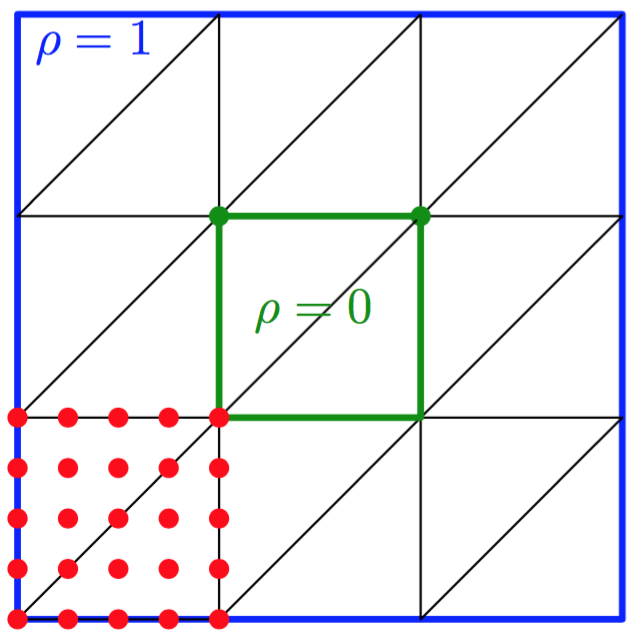
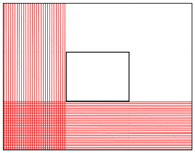
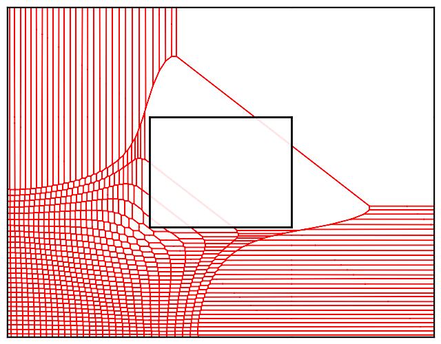
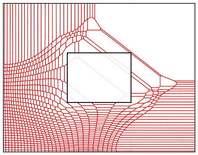
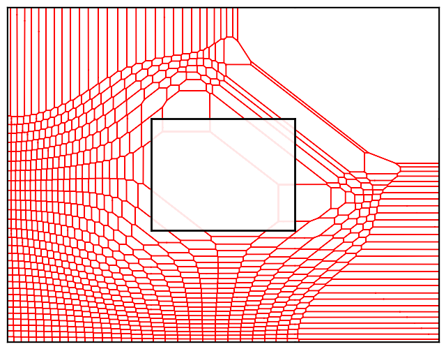
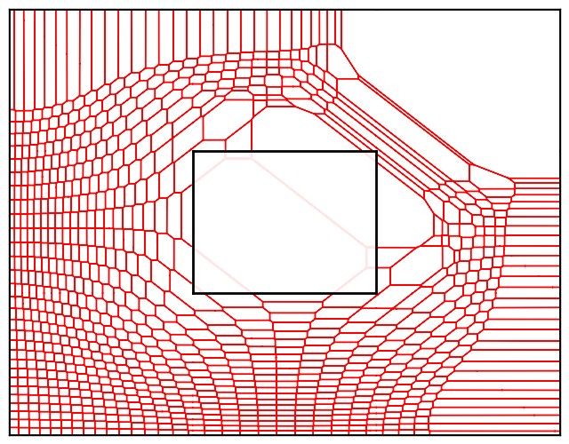
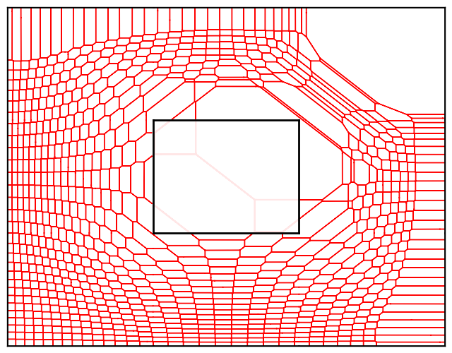
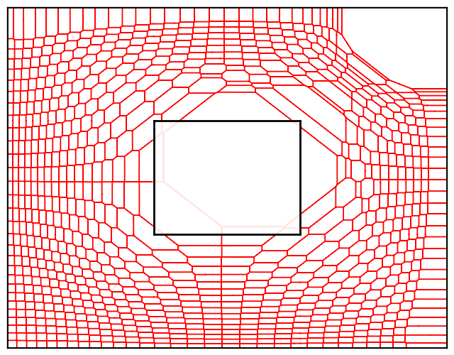
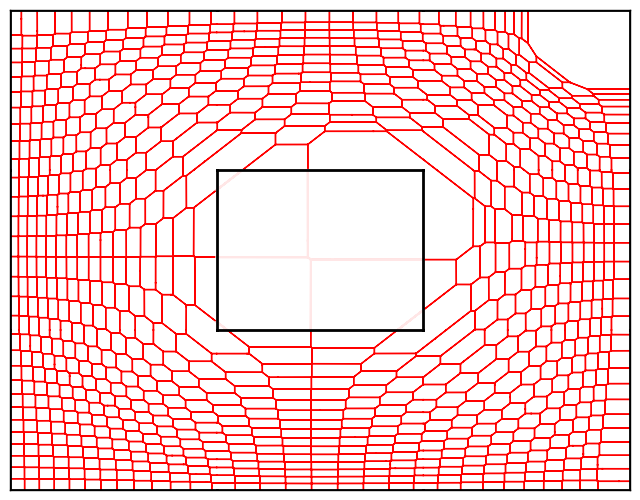
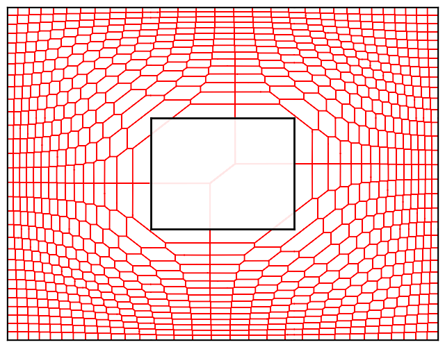
Figure 3. Evolution of the Laguerre cells during the execution of the damped Newton algorithm for semi-discrete optimal transport. (Top) The source density $\rho$ is piecewise linear over the domain $X=[0,3]^{3}$ over the displayed triangulation: it takes value $1$ on the boundary of the square $[0,3]^{2}$ and $0$ on the boundary of $[1,2]^{2}$. The target measure is uniform over a $30^{2}$ uniform grid in $[0,1]^{2}$. (Bottom) Laguerre cells at steps $k=0,2,6,9,12,15,18,21$ and $25$.

Appendix A A weighted Poincaré-Wirtinger inequality

In this section, we provide an (almost) explicit example of a probability density on $\mathbb{R}^{d}$ whose support is an annulus, therefore not simply connected, but which still satisfies a weighted Poincaré-Wirtinger inequality.

Proposition A.1.

Let $0<r<R$ and assume that $\overline{\rho}\in\mathcal{C}^{0}([0,R])$ is a probability density with $\overline{\rho}=0$ on $[0,r]$ and $\overline{\rho}$ concave on $[r,R]$. Consider

$$\rho(x)=\frac{1}{\left\|x\right\|^{d-1}\omega_{d-1}}\overline{\rho}(\left\|x\right\|)\qquad\hbox{over}\qquad X:=\mathrm{B}(0,R)\subseteq\mathbb{R}^{d},$$

where $\omega_{d-1}$ is the volume of the unit sphere $\mathbb{S}^{d-1}$. Then, $\rho$ satisfies the weighted Poincaré-Wirtinger inequality (PW) for some positive constant.

The proof relies on two $L^{1}$-Poincaré-Wirtinger inequalities. The first inequality is the usual Poincaré-Wirtinger inequality on the sphere: given a $\mathcal{C}^{1}$ function $f$ on $\mathbb{S}^{d-1}$, and $F_{d-1}:=(1/\omega_{d-1})\int_{\mathbb{S}^{d-1}}f(z)\mathrm{d}z$,

$$\int_{\mathbb{S}^{d-1}}\left|f(z)-F_{d-1}\right|\mathrm{d}\mathcal{H}^{d-1}(z)\leqslant c_{d}\int_{\mathbb{S}^{d-1}}\left\|\nabla f(z)\right\|\mathrm{d}\mathcal{H}^{d-1}(z)$$ (A.51)

for some positive constant $c_{d}$. The second inequality is a Poincaré-Wirtinger inequality on the segment $[0,R]$ weighted by $\overline{\rho}$. Given a function in $\mathcal{C}^{1}([0,R])$, and letting $F_{1}:=\int_{0}^{R}f(r)\overline{\rho}(r)\mathrm{d}r/\int_{0}^{R}\overline{\rho}(r)\mathrm{d}r$,

$$\int_{0}^{R}\left|\overline{f}(r)-F_{1}\right|\overline{\rho}(r)\mathrm{d}r\leqslant c_{\overline{\rho}}\int_{0}^{R}\left|\overline{f}^{\prime}(r)\right|\overline{\rho}(r)\mathrm{d}r$$ (A.52)

for some positive constant $c_{\overline{\rho}}$ depending only on $\overline{\rho}$. The inequality (A.52) can be deduced from Theorem 2.1 in [3] and from the concavity of $\overline{\rho}$ on $[r,R]$.

Proof.

We now proceed to the proof of the Poincaré-Wirtinger inequality for $(X,\rho)$. Let $f:\mathrm{B}(0,R)\to\mathbb{R}$ be a function of class $\mathcal{C}^{1}$. By polar coordinates and the definition of $\rho$, one has

$$F :=\int_{\mathrm{B}(0,R)}f(x)\rho(x)\mathrm{d}\mathcal{H}^{d}(x)$$

$$=\int_{0}^{R}\frac{1}{\omega_{d-1}r^{d-1}}\int_{\mathbb{S}^{d-1}(r)}f(z)\overline{\rho}(r)\mathrm{d}\mathcal{H}^{d-1}(z)\mathrm{d}r=\int_{0}^{R}\overline{f}(r)\overline{\rho}(r)\mathrm{d}r,$$

where the function $\overline{f}(r)$ is the mean value of $f$ over the sphere $\mathbb{S}^{d-1}(r)$,

$$\overline{f}(r)=\frac{1}{\omega_{d-1}r^{d-1}}\int_{\mathbb{S}^{d-1}(r)}f(z)\mathrm{d}\mathcal{H}^{d-1}(z)=\frac{1}{\omega_{d-1}}\int_{\mathbb{S}^{d-1}}f(rz)\mathrm{d}\mathcal{H}^{d-1}(z).$$

Using the triangle inequality and the relation between $\overline{\rho}$ and $\rho$ we get

$$\int_{\mathrm{B}(0,R)}\left|f(x)-F\right|\rho(x)\mathrm{d}\mathcal{H}^{d}(x)=\int_{0}^{R}\int_{\mathbb{S}^{d-1}(r)}\left|f(z)-F\right|\rho(z)\mathrm{d}\mathcal{H}^{d-1}(z)\mathrm{d}r$$

$$\quad\leqslant\int_{0}^{R}\overline{\rho}(r)\left|\overline{f}(r)-F\right|\mathrm{d}r+\int_{0}^{R}\frac{\overline{\rho}(r)}{r^{d-1}\omega_{d-1}}\int_{\mathbb{S}^{d-1}(r)}\left|f(z)-\overline{f}(r)\right|\mathrm{d}\mathcal{H}^{d-1}(z)\mathrm{d}r$$ (A.53)

We first deal with the second term of the sum. Using the Poincaré-Wirtinger inequality on the sphere (A.51), we have

$$\int_{\mathbb{S}^{d-1}(r)}\left|f(z)-\overline{f}(r)\right|\mathrm{d}\mathcal{H}^{d-1}(z)\leqslant c_{d}\int_{\mathbb{S}^{d-1}(r)}\left\|\left.\nabla f(z)\right|_{z^{\perp}}\right\|\mathrm{d}\mathcal{H}^{d-1}(z),$$

where $\left.\nabla f(z)\right|_{z^{\perp}}$ is the orthogonal projection of the gradient on the tangent plane $\{z\}^{\perp}$, so that

$$\int_{0}^{R}\frac{\overline{\rho}(r)}{r^{d-1}\omega_{d-1}}\int_{\mathbb{S}^{d-1}(r)}\left|f(z)-\overline{f}(r)\right|\mathrm{d}\mathcal{H}^{d-1}(z)\leqslant c_{d}\int_{B(0,r)}\left\|\left.\nabla f(x)\right|_{x^{\perp}}\right\|\rho(x)\mathrm{d}\mathcal{H}^{d}(x).$$ (A.54)

By the calculation of $F$ above, we see $F$ is also the mean value of $\overline{f}$ weighted by $\overline{\rho}$. We can therefore control the first term of the upper bound of (A.53) using the Poincaré-Wirtinger inequality on the segment (A.52):

$$\int_{0}^{R}\overline{\rho}(r)\left|\overline{f}(r)-F\right|\mathrm{d}r\leqslant c_{\overline{\rho}}\int_{0}^{R}\left|\overline{f}^{\prime}(r)\right|\overline{\rho}(r)\mathrm{d}r.$$

Now, notice that:

$$\overline{f}^{\prime}(r)=\lim_{h\to 0}\frac{\overline{f}(r+h)-\overline{f}(r)}{h}=\lim_{h\to 0}\frac{1}{\omega_{d-1}}\int_{\mathbb{S}^{d-1}}\frac{f((r+h)z)-f(rz)}{h}\mathrm{d}\mathcal{H}^{d-1}(z),$$

from which we deduce

$$\left|\overline{f}^{\prime}(r)\right|\leqslant\frac{1}{\omega_{d-1}}\int_{\mathbb{S}^{d-1}}\left|\frac{\partial f}{\partial r}(rz)\right|\mathrm{d}\mathcal{H}^{d-1}(z)=\frac{1}{\omega_{d-1}r^{d-1}}\int_{\mathbb{S}^{d-1}(r)}\left|\langle\nabla f(z)\mid\frac{z}{r}\rangle\right|\mathrm{d}\mathcal{H}^{d-1}(z)$$

Integrating this inequality shows that

$$\int_{0}^{R}\overline{\rho}(r)\left|\overline{f}(r)-F\right|\mathrm{d}r \leqslant c_{\overline{\rho}}\int_{0}^{R}\frac{\overline{\rho}(r)}{\omega_{d-1}r^{d-1}}\int_{\mathbb{S}^{d-1}(r)}\left|\langle\nabla f(z)\mid\frac{z}{r}\rangle\right|\mathrm{d}\mathcal{H}^{d-1}(z)$$

$$=c_{\overline{\rho}}\int_{\mathrm{B}(0,R)}\left|\langle\nabla f(x)\mid\frac{x}{\left\|x\right\|}\rangle\right|\rho(x)\mathrm{d}\mathcal{H}^{d}(x).$$ (A.55)

From the simple inequality $(a+b)^{2}\leqslant 2(a^{2}+b^{2})$, we get

$$\left|\langle\nabla f(x)\mid\frac{x}{\left\|x\right\|}\rangle\right|+\left\|\left.\nabla f(x)\right|_{x^{\perp}}\right\|\leqslant\sqrt{2}\left\|\nabla f(x)\right\|.$$

Using the bounds (A.54) and (A.55) in Equation (A.53), we get the desired inequality:

$$\int_{\mathrm{B}(0,R)}\left|f(x)-F\right|\rho(x)\mathrm{d}\mathcal{H}^{d}(x)\leqslant\sqrt{2}(c_{d}+c_{\overline{\rho}})\int_{\mathrm{B}(0,R)}\left\|\nabla f(x)\right\|\rho(x)\mathrm{d}\mathcal{H}^{d}(x).\qed$$

Appendix B Proof of Theorem 3.1

B.1. Existence of partial derivatives

Without loss of generality, we assume that $\bm{\lambda}_{0}=\bm{0}$. We start the proof of Theorem 3.1 by showing the existence of partial derivatives for the map $\hat{G}$. In this section, we denote $e_{1},\ldots,e_{N}$ the canonical basis of $\mathbb{R}^{N}$. We start by rewriting the finite difference defining the partial derivative of $\hat{G}$ in direction $e_{i}$ using the coarea formula. Fix $\left\|\bm{\lambda}\right\|<T_{tr}$. For $t>0$, one has:

$$\frac{1}{t}(\hat{G}(\bm{\lambda}+t\bm{e}_{i})-\hat{G}(\bm{\lambda})) =\frac{1}{t}\int_{K(\bm{\lambda}+t\bm{e}_{i})\setminus K(\bm{\lambda})}\hat{\rho}(x)\mathrm{d}\mathcal{H}^{d}(x)$$

$$=\frac{1}{t}\int_{\lambda_{i}}^{\lambda_{i}+t}\hat{g}(s)\mathrm{d}s,$$ (B.56)

where the function $\hat{g}$ is defined by

$$\hat{g}(s):=\int_{\cap_{j\neq i}K_{j}(\lambda_{j})\cap f_{i}^{-1}(s)}\frac{\hat{\rho}(x)}{\left\|\nabla f_{i}(x)\right\|}\mathrm{d}\mathcal{H}^{d-1}(x).$$ (B.57)

The same reasoning also holds for $t<0$. We now claim that $\hat{g}$ is continuous on some interval around $\lambda_{i}$, which by (B.56) and the Fundamental Theorem of Calculus will imply that the limit as $t\to 0$ in (B.56) exists and is equal to $\hat{g}(\bm{\lambda})$, thus establishing the formula (3.14). The continuity of $\hat{g}$ follows from the next proposition, which is formulated in a slightly more general way.

Proposition B.1.

Let $\sigma$ be a continuous non-negative function on $\hat{X}$ and let $\omega$ be the modulus of continuity of $\sigma$. Given any vector $\bm{\lambda}$ in $\mathbb{R}^{N}$ with $\left\|\bm{\lambda}\right\|_{\infty}\leqslant T_{tr}$, consider the function

$$h:s\in\mathbb{R}\mapsto\int_{L\cap S_{s}}\sigma(x)\mathrm{d}\mathcal{H}^{d-1}(x),$$

where $L:=\bigcap_{j\neq i}K_{j}(\lambda_{j})$ and $S_{s}:=f_{i}^{-1}(s)$. Then $h$ is uniformly continuous on $[-T_{tr},T_{tr}]$ and has modulus of continuity

$$\omega_{h}(\delta)=C_{1}\cdot(\omega(C_{2}\delta)+\left|\delta\right|),$$ (B.58)

where the constants only depend on $\left\|f_{i}\right\|_{\mathcal{C}^{1,1}}$, $\operatorname{diam}(\hat{X})$, $\varepsilon_{nd}$, $\varepsilon_{tr}$ and $\left\|\sigma\right\|_{\infty}$.

Taking $\sigma=\hat{\rho}/\left\|\nabla f_{i}\right\|$ in the previous proposition, which is continuous using the non-degeneracy condition (ND) and the assumption $f_{i}\in\mathcal{C}^{1,1}(\hat{X})$, we see that the function $\hat{g}$ defined by (B.57) is continuous. This implies the existence of partial derivatives and establishes formula (3.14). The proof of Proposition B.1 requires the following lemma.

Lemma B.2.

Assume that the functions $f_{i}:\hat{X}\to\mathbb{R}$ satisfy (ND). Then, for every $i\in\{1,\ldots,N\},$ there exists a map $\Phi_{i}:\hat{X}\times\mathbb{R}\to\mathbb{R}^{d}$ such that:

1. For any $(x,t)$ in $\hat{X}\times\mathbb{R}$ such that the curve $\Phi_{i}(x,[0,t])$ remains in $\hat{X}$, one has $f_{i}(\Phi_{i}(x,t))=f_{i}(x)+t$.

2. The map $\Phi_{i}$ satisfies the following inequalities for every $x,y\in\hat{X}$, $t\in\mathbb{R}$:

   $$\left\|\Phi_{i}(x,t)-\Phi_{i}(x,s)\right\|\leqslant\frac{\left|t-s\right|}{\varepsilon_{nd}}$$ (B.59)

   $$\left\|\Phi_{i}(x,t)-\Phi_{i}(y,t)\right\|\leqslant\exp(C_{\Phi}\left|t\right|)\left\|x-y\right\|,$$ (B.60)

   where $C_{\Phi}:=3C_{L}/\varepsilon_{nd}^{2}$.

Proof.

We consider the vector field $V_{i}^{0}(x)=\nabla f_{i}(x)/\left\|\nabla f_{i}(x)\right\|^{2}$ on $\hat{X}$, which satisfies $\left\|V_{i}^{0}\right\|_{\infty}\leqslant 1/\varepsilon_{nd}$ and whose Lipschitz constant is bounded by $C_{\Phi}$. This vector field is extended to $\mathbb{R}^{d}$ using the orthogonal projection on $\hat{X}$, denoted $p_{\hat{X}}$,

$$\forall x\in\mathbb{R}^{d},~{}V_{i}(x):=V^{0}_{i}(p_{\hat{X}}(x)).$$

By convexity of $\hat{X}$, the map $p_{\hat{X}}$ is $1$-Lipschitz. This implies that the Lipschitz constant of $V_{i}$ is also bounded by $C_{\Phi}$. We let $\Phi_{i}$ be the flow induced by this vector field, which exists and is for all time since $V_{i}$ is bounded and uniformly Lipschitz on all of $\mathbb{R}^{d}$. The inequality (B.59) follows from the definition of integral curves and the bound on $\left\|V_{i}\right\|$. Any integral curve $\gamma:[0,T]\to\mathbb{R}^{d}$ of $V_{i}$ which remains in $\hat{X}$ satisfies

$$f_{i}(\gamma(t)) =f_{i}(\gamma(0))+\int_{0}^{t}\langle\gamma^{\prime}(s)\mid\nabla f_{i}(\gamma(s))\rangle\mathrm{d}s$$

$$=f_{i}(\gamma(0))+\int_{0}^{t}\langle V_{i}(\gamma(s))\mid\nabla f_{i}(\gamma(s))\rangle\mathrm{d}s=f_{i}(\gamma(0))+t,$$

thus establishing (i). The inequality (B.60) follows from the bound on the Lipschitz constant of $V_{i}$ and from Gronwall’s lemma. ∎

Figure 4. Illustration of the proof of Proposition B.1.

Proof of Proposition B.1.

Let $t,s$ be small enough so that the transversality condition (T) holds (that is $t,s\in[-T_{tr},T_{tr}]$). We assume that $t<s$ so as to fix the signs of some expressions. We consider the following partition of the facet $S_{t}\cap L$, whose geometric meaning is illustrated in Figure 4:

$$A_{t}=\{x\in S_{t}\cap L\mid\Phi_{i}(x,[0,s-t])\subseteq L\}$$

$$B_{t}=\{x\in S_{t}\cap L\mid\exists u\in[0,s-t),~{}\Phi_{i}(x,u)\in\partial L\}.$$

Similarly, we define

$$A_{s}=\{x\in S_{s}\cap L\mid\Phi_{i}(x,[t-s,0])\subseteq L\}$$

$$B_{s}=\{x\in S_{s}\cap L\mid\exists u\in(t-s,0],~{}\Phi_{i}(x,u)\in\partial L\}.$$

Recall that by definition,

$$h(t)=\int_{A_{t}}\sigma(x)\mathrm{d}\mathcal{H}^{d-1}(x)+\int_{B_{t}}\sigma(x)\mathrm{d}\mathcal{H}^{d-1}(x),$$ (B.61)

where the integral is with respect to the $(d-1)$-dimensional Hausdorff measure. Our strategy to show the continuity of $h$ is to prove that the first term in the sums defining $h(t)$ and $h(s)$ in (B.61) are close, namely

$$\left|\int_{A_{t}}\sigma(x)\mathrm{d}\mathcal{H}^{d-1}(x)-\int_{A_{s}}\sigma(x)\mathrm{d}\mathcal{H}^{d-1}(x)\right|\leqslant C_{3}\cdot(\left|s-t\right|+\omega(C\left|s-t\right|))$$ (B.62)

and then that the terms involving $B_{t},B_{s}$ are small (recall that both sets depend on $t$ and $s$):

$$\int_{B_{t}}\left|\sigma(x)\mathrm{d}\mathcal{H}^{d-1}(x)\right|+\int_{B_{s}}\left|\sigma(x)\mathrm{d}\mathcal{H}^{d-1}(x)\right|\leqslant C_{4}\cdot\left|s-t\right|$$ (B.63)

The combination of the estimates (B.62) and (B.63) implies the desired inequality (B.58). We now turn to the proof of these estimates, and that the constants $C_{3}$ and $C_{4}$ in these estimates depend on $\left\|f_{i}\right\|_{\mathcal{C}^{1,1}}$, $\operatorname{diam}(\hat{X})$, $\varepsilon_{nd}$, $\varepsilon_{tr}$ and $\left\|\sigma\right\|_{\infty}$.

Proof of Estimate (B.62). By Lemma B.2.(i), for any point $x$ in $A_{t}$ one has $f_{i}(\Phi_{i}(x,s-t))=s$, so that the map $F(x):=\Phi_{i}(x,s-t)$ induces a bijection between the sets $A_{t}$ and $A_{s}$. As a consequence of (B.60), the restriction of $F$ to $A_{t}$ is a bi-Lipschitz bijection between the sets $A_{t}$ and $A_{s}$, with Lipschitz constant

$$\max\{\left\|F^{-1}\right\|_{\operatorname{Lip}(A_{s})},\ \left\|F\right\|_{\operatorname{Lip}(A_{t})}\}\leqslant\exp(C_{\Phi}\left|s-t\right|).$$

Using a Lipschitz change of variable formula, we get

$$\int_{A_{t}}\sigma(x)\mathrm{d}\mathcal{H}^{d-1}(x) =\int_{F^{-1}(A_{s})}\sigma(x)\mathrm{d}\mathcal{H}^{d-1}(x)$$

$$\leqslant\left\|F^{-1}\right\|_{\operatorname{Lip}(A_{s})}^{d-1}\int_{A_{s}}\sigma(F^{-1}(x))\mathrm{d}\mathcal{H}^{d-1}(x)$$

$$\leqslant\exp(C_{\Phi}(d-1)\left|s-t\right|)\int_{A_{s}}\sigma(F^{-1}(x))\mathrm{d}\mathcal{H}^{d-1}(x).$$ (B.64)

By definition of the modulus of continuity and thanks to (B.59),

$$\left|\sigma(F^{-1}(x))-\sigma(x)\right| \leqslant\omega(\left\|F^{-1}(x)-x\right\|)$$

$$=\omega(\left\|\Phi(x,s-t)-x\right\|)\leqslant\omega(\left|s-t\right|/\varepsilon_{nd})$$

Integrating this inequality, we get

$$\int_{A_{s}}\sigma(F^{-1}(x))\mathrm{d}\mathcal{H}^{d-1}(x) \leqslant\int_{A_{s}}\sigma(x)\mathrm{d}\mathcal{H}^{d-1}(x)+\mathcal{H}^{d-1}(A_{s})\omega(\left|s-t\right|/\varepsilon_{nd})$$

$$\leqslant\int_{A_{s}}\sigma(x)\mathrm{d}\mathcal{H}^{d-1}(x)+\mathcal{H}^{d-1}(\hat{X})\omega(\left|s-t\right|/\varepsilon_{nd})$$ (B.65)

where the second inequality uses the monotonicity of the $(d-1)$-dimensional Hausdorff measure of the boundary of a convex set with respect to inclusion, see [32, p.211]. Combining (B.64) and (B.65) we get

$$\int_{A_{t}}\sigma(x)\mathrm{d}\mathcal{H}^{d-1}(x)\leqslant\exp(C_{\Phi}(d-1)\left|s-t\right|)\left(\int_{A_{s}}\sigma(x)\mathrm{d}\mathcal{H}^{d-1}(x)+\mathcal{H}^{d-1}(\hat{X})\omega(\left|s-t\right|/\varepsilon_{nd})\right)$$

so that

$$\int_{A_{t}}\sigma(x)\mathrm{d}\mathcal{H}^{d-1}(x)-\int_{A_{s}}\sigma(x)\mathrm{d}\mathcal{H}^{d-1}(x) \leqslant(\exp(C_{\Phi}(d-1)\left|s-t\right|)-1)\left\|\sigma\right\|_{\infty}\mathcal{H}^{d-1}(\hat{X})+$$

$$\qquad\exp(C_{\Phi}(d-1)\left|s-t\right|)\mathcal{H}^{d-1}(\hat{X})\omega(\left|s-t\right|/\varepsilon_{nd})$$

$$\leqslant C_{3}\cdot(\left|s-t\right|+\omega(\left|s-t\right|/\varepsilon_{nd})),$$

where the constant $C_{3}$ depends on $C_{L}$, $\varepsilon_{nd}$, $\varepsilon_{tr}$, $\left\|\sigma\right\|_{\infty}$ and $\operatorname{diam}(\hat{X})$. Exchanging the role of $s$ and $t$ completes the proof of (B.62).

Proof of (B.63). By definition, for every point $x$ in the set $B_{t}$, the curve $\Phi_{i}(x,[0,s-t])$ must cross the boundary of $L$ at some point, so that

$$u(x):=\min\{v\in[0,s-t]\mid\Phi_{i}(x,v)\in\partial L\}$$

is well defined. We write $P(x):=\Phi_{i}(x,u(x))$ for the corresponding point on the boundary of $L$. By definition of $u(x)$, the curve $\Phi(x,[0,u(x)])$ is included in $L$, so that by Lemma B.2.(i) we have $f_{i}(P(x))=t+u(x)$. This shows

$$P(B_{t})\subseteq\Lambda:=\partial L\cap f_{i}^{-1}([t,s]).$$ (B.66)

We now prove that the map $P$ satisfies a reverse-Lipschitz inequality. Note that for any point $x$ in $B_{t}$,

$$x=\Phi_{i}(P(x),-u(x))=\Phi_{i}(P(x),t-f_{i}(P(x))),$$

Using the bounds (B.60) and (B.59), we get that for any $x,y$ in $B_{t}$,

$$\left\|x-y\right\| \leqslant\left\|\Phi_{i}(P(x),t-f_{i}(P(x)))-\Phi_{i}(P(y),t-f_{i}(P(y)))\right\|$$

$$\leqslant\left\|\Phi_{i}(P(x),t-f_{i}(P(x)))-\Phi_{i}(P(y),t-f_{i}(P(x)))\right\|$$

$$\qquad\qquad+\left\|\Phi_{i}(P(y),t-f_{i}(P(x)))-\Phi_{i}(P(y),t-f_{i}(P(y)))\right\|$$

$$\leqslant\exp(C_{\Phi}T_{tr})\left\|P(x)-P(y)\right\|+\left|f_{i}(P(x))-f_{i}(P(y))\right|/\varepsilon_{nd}$$

$$\leqslant C^{\prime}\left\|P(x)-P(y)\right\|$$

where $C^{\prime}:=\exp(C_{\Phi})+C_{L}/\varepsilon_{nd}$; we have used that $T_{tr}\leqslant 1$. We can now bound the $(d-1)$–Hausdorff measure of $B_{t}$ from that of $\Lambda$ using this Lipschitz bound and the inclusion (B.66):

$$\mathcal{H}^{d-1}(B_{t})\leqslant\mathcal{H}^{d-1}(P^{-1}(P(B_{t})))\leqslant C^{\prime d-1}\mathcal{H}^{d-1}(\Lambda).$$ (B.67)

What remains to be done is to prove that the $(d-1)$–Hausdorff measure of $\Lambda$ behaves like $\operatorname{O}(\left|s-t\right|)$, and this is where the transversality condition will enter.

Let us write

$$F_{j}:=\begin{cases}f_{j}^{-1}(\lambda_{j}),&j\neq 0,i,\\ \partial\hat{X}\cap\partial L,&j=0.\end{cases}$$

Then $\partial L$ can be partitioned (up to a $\mathcal{H}^{d-1}$–negligible set) into faces $\partial L=\cup_{j\neq i}(F_{j}\cap L)$ and using the coarea formula on each of the facets we get (writing $B:=f_{i}^{-1}([t,s])$)

$$\mathcal{H}^{d-1}(\Lambda) =\sum_{j\neq i}\mathcal{H}^{d-1}(B\cap(F_{j}\cap L))$$

$$=\sum_{j\neq i}\int_{B\cap(F_{j}\cap L)}\mathrm{d}\mathcal{H}^{d-1}(x)$$

$$=\sum_{j\neq i}\int_{t}^{s}\int_{S_{u}\cap(F_{j}\cap L)}\frac{1}{J_{ij}(x)}\mathrm{d}\mathcal{H}^{d-2}(x)\mathrm{d}u,$$ (B.68)

where and $J_{ij}(x)$ is the Jacobian of the restriction of the function $f_{i}$ to the hypersurface $F_{j}$. More precisely,

$$J_{ij}(x)=\left\|\nabla f_{i}(x)-\langle\nabla f_{i}(x)\mid\nabla f_{j}(x)\rangle\frac{\nabla f_{j}(x)}{\left\|\nabla f_{j}(x)\right\|^{2}}\right\|$$

if $j\neq 0$, $i$, and

$$J_{i0}(x)=\left\|\nabla f_{i}(x)-\langle\nabla f_{i}(x)\mid v_{0}(x)\rangle v_{0}(x)\right\|$$

where $v_{0}(x)\in\mathcal{N}_{x}\hat{X}$ is a unit vector. Since $\hat{X}$ is convex, for $\mathcal{H}^{d-1}$ a.e. $x\in\partial\hat{X}$, the normal cone $\mathcal{N}_{x}\hat{X}$ consists of only one direction, thus for such $x$ there is a unique choice of $v_{0}(x)$. Let us write $v_{i}=\nabla f_{i}(x)/\left\|\nabla f_{i}(x)\right\|$ and $v_{j}$ for either $\nabla f_{j}(x)/\left\|\nabla f_{j}(x)\right\|$ or $v_{0}(x)$, we then have using (T)

$$J_{ij}(x)^{2} =\left\|\nabla f_{i}(x)\right\|^{2}\left\|v_{i}-\langle v_{i}\mid v_{j}\rangle v_{j}\right\|^{2}$$

$$\geqslant\left\|\nabla f_{i}(x)\right\|^{2}(1-\langle v_{i}\mid v_{j}\rangle^{2})$$

$$\geqslant\varepsilon^{2}_{nd}\varepsilon^{2}_{tr}.$$ (B.69)

Combining (B.68) and (B.69) gives us

$$\mathcal{H}^{d-1}(\Lambda) \leqslant\frac{1}{\varepsilon_{nd}\varepsilon_{tr}}\sum_{j\neq i}\int_{t}^{s}\mathcal{H}^{d-2}(S_{u}\cap(F_{j}\cap L))\mathrm{d}u$$

$$=\frac{1}{\varepsilon_{nd}\varepsilon_{tr}}\int_{t}^{s}\mathcal{H}^{d-2}(S_{u}\cap\partial L)\mathrm{d}u.$$ (B.70)

By definition, a point belongs to the intersection $S_{u}\cap\partial L$ if it lies in the singularity set $\Sigma(\bm{\lambda}(u))$ where $\bm{\lambda}(u)=(\lambda_{1},\ldots,\lambda_{i-1},u,\lambda_{i+1},\ldots,\lambda_{N})$. By Lemma 3.2,

$$\mathcal{H}^{d-2}(S_{u}\cap\partial L)\leqslant\mathcal{H}^{d-2}(\Sigma(\bm{\lambda}(u)))\leqslant C(d,\operatorname{diam}(\hat{X}))\cdot\frac{1}{\varepsilon_{tr}}.$$ (B.71)

Combining (B.67), (B.70) and (B.71) we obtain $\mathcal{H}^{d}(B_{t})\leqslant C\cdot\left|t-s\right|$, which implies (B.63) using the boundedness of $\sigma$. ∎

B.2. Continuity of partial derivatives

We prove that the function $\hat{G}$ defined in (3.12) is continuously differentiable by controlling the modulus of continuity of its partial derivatives given in (3.14). Again, we start with a slightly more general proposition.

Proposition B.3.

Let $\sigma$ be a continuous function on $\hat{X}$ with modulus of continuity $\omega$ and $i\in\{1,\cdots,N\}$. Consider the following function on the cube $Q:=[-T_{tr},T_{tr}]^{N}$:

$$H(\bm{\lambda}):=\int_{K(\bm{\lambda})\cap f_{i}^{-1}(\lambda_{i})}\sigma(x)\mathrm{d}\mathcal{H}^{d-1}(x).$$

Then $H$ is uniformly continuous on $Q$ with modulus of continuity

$$\omega_{H}(\delta)=C_{1}\cdot(\omega(C_{2}\delta)+\left|\delta\right|),$$

where the constants only depend on $\left\|f_{i}\right\|_{\mathcal{C}^{1,1}(\hat{X})}$, $\operatorname{diam}(\hat{X})$, $\varepsilon_{nd}$, $\varepsilon_{tr}$, and $\left\|\sigma\right\|_{\infty}$.

Proof.

Proposition B.1 yields that the function $H$ is uniformly continuous with respect to changes of the $i$th variable. Let us now consider variations with respect to the $j$th variable, with $j\neq i$ by introducing

$$h:s\in[-T_{tr},T_{tr}]\mapsto\int_{K(\lambda_{1},\ldots,\lambda_{j-1},s,\lambda_{j+1},\ldots,\lambda_{N})\cap f_{i}^{-1}(\lambda_{i})}\sigma(x)\mathrm{d}\mathcal{H}^{d-1}(x).$$

for some fixed $\bm{\lambda}\in[-T_{tr},T_{tr}]^{N}$. We can rewrite the difference between two values of $h$ using the coarea formula. As before, we assume $s>t$ to fix the signs and introduce $L^{\prime}:=\hat{X}\cap\bigcap_{k\not\in\{i,j\}}K_{k}(\lambda_{k})$ and $S:=f_{i}^{-1}(\lambda_{i})$. We have

$$h(s)-h(t) =\int_{L^{\prime}\cap K_{j}(s)\cap S}\sigma(x)\mathrm{d}\mathcal{H}^{d-1}(x)-\int_{L^{\prime}\cap K_{j}(t)\cap S}\sigma(x)\mathrm{d}\mathcal{H}^{d-1}(x)$$

$$=\int_{t}^{s}\int_{L^{\prime}\cap S\cap f_{j}^{-1}(u)}\frac{\sigma(x)}{J_{ij}(x)}\mathrm{d}\mathcal{H}^{d-2}(x)\mathrm{d}u,$$

where the Jacobian factor $J_{ij}\geqslant\varepsilon_{nd}\varepsilon_{tr}$ from (B.69). Therefore,

$$h(s)\leqslant h(t)+\frac{\left\|\sigma\right\|_{\infty}}{\varepsilon_{nd}\varepsilon_{tr}}\int_{t}^{s}\mathcal{H}^{d-2}(L\cap S\cap f^{-1}(u))\mathrm{d}u.$$ (B.72)

Just as in the proof of Proposition B.1, the set $L\cap S\cap f^{-1}(u)$ is included in the set $\Sigma(\lambda_{1},\ldots,\lambda_{j-1},u,\lambda_{j},\ldots,\lambda_{N})$. Thus, by Lemma 3.2,

$$\mathcal{H}^{d-2}(L\cap S\cap f^{-1}(u))\leqslant\frac{C(d,\hat{X})}{\varepsilon_{tr}}.$$ (B.73)

Combining (B.72) and (B.73) we can see that the function $h$ is Lipschitz with constant

$$C_{h}:=C(d,\hat{X})\frac{\left\|\sigma\right\|_{\infty}}{\varepsilon_{nd}\varepsilon_{tr}^{2}}.$$

Finally,

$$\left|H(\bm{\mu})-H(\bm{\lambda})\right| \leqslant\sum_{j=1}^{N}\left|H(\lambda_{1},\ldots,\lambda_{k-1},\mu_{j},\ldots,\mu_{N})-H(\lambda_{1},\ldots,\lambda_{j},\mu_{j+1},\ldots,\mu_{N})\right|$$

$$\leqslant\omega_{h}(\left|\mu_{i}-\lambda_{i}\right|)+\sum_{j\neq i}C_{h}\left|\mu_{j}-\lambda_{j}\right|$$

$$\leqslant\omega_{h}(\left\|\mu-\lambda\right\|_{\infty})+(N-1)C_{h}\left\|\mu-\lambda\right\|_{\infty},$$

where $\omega_{h}$ is the modulus of continuity defined in Proposition B.1. This establishes the uniform continuity of the function $H$, with the desired modulus of continuity. ∎

B.3. Proof of Theorem 3.1

Proposition B.1 shows that the partial derivative $\hat{G}$ with respect to the variable $\lambda_{i}$ exists and that its expression is given by (B.57). Applying Proposition B.3 with $\sigma(x)=\hat{\rho}(x)/\left\|\nabla f_{i}(x)\right\|$, we obtain $\mathcal{C}^{0,\alpha}$ regularity for each of the partial derivatives of $\hat{G}$ on the cube $Q:=[-T_{tr},T_{tr}]^{N}$ from the $\mathcal{C}^{0,\alpha}$ regularity of $\hat{\rho}$. Moreover, the $\mathcal{C}^{0,\alpha}$ constant of each partial derivative over $Q$ is controlled by

$$C(\operatorname{diam}(\hat{X}),\varepsilon_{nd},\varepsilon_{tr},\left\|\nabla f_{i}\right\|_{\mathcal{C}^{1,1}(X)},\left\|\hat{\rho}\right\|_{\mathcal{C}^{0,\alpha}(X)}).$$

References

- [1] Cgal, Computational Geometry Algorithms Library, http://www.cgal.org.
- [2] Geograml, a programming library of geometric algorithms, http://alice.loria.fr/software/geogram/doc/html/.
- [3] Gabriel Acosta and Ricardo G Durán, An optimal poincaré inequality in for convex domains, Proceedings of the American Mathematical Society (2004), 195–202.
- [4] Hedy Attouch, Giuseppe Buttazzo, and Gérard Michaille, Variational analysis in sobolev and bv spaces: applications to pdes and optimization, vol. 17, Siam, 2014.
- [5] F. Aurenhammer, F. Hoffmann, and B. Aronov, Minkowski-type theorems and least-squares clustering, Algorithmica 20 (1998), no. 1, 61–76.
- [6] Jean-David Benamou, Brittany D Froese, and Adam M Oberman, Numerical solution of the optimal transportation problem using the monge–ampere equation, Journal of Computational Physics 260 (2014), 107–126.
- [7] Luis A. Caffarelli, The regularity of mappings with a convex potential, J. Amer. Math. Soc. 5 (1992), no. 1, 99–104. MR 1124980 (92j:35018)
- [8] Luis A Caffarelli, Sergey A Kochengin, and Vladimir I Oliker, Problem of reflector design with given far-field scattering data, Monge Ampère Equation: Applications to Geometry and Optimization: NSF-CBMS Conference on the Monge Ampère Equation, Applications to Geometry and Optimization, July 9-13, 1997, Florida Atlantic University, vol. 226, American Mathematical Soc., 1999, p. 13.
- [9] Guillaume Carlier, Alfred Galichon, and Filippo Santambrogio, From knothe’s transport to brenier’s map and a continuation method for optimal transport, SIAM Journal on Mathematical Analysis 41 (2010), no. 6, 2554–2576.
- [10] Pedro Machado Manhaes De Castro, Quentin Mérigot, and Boris Thibert, Intersection of paraboloids and application to minkowski-type problems, Proceedings of the thirtieth annual symposium on Computational geometry, ACM, 2014, p. 308.
- [11] Fernando de Goes, Katherine Breeden, Victor Ostromoukhov, and Mathieu Desbrun, Blue noise through optimal transport, ACM Transactions on Graphics (TOG) 31 (2012), no. 6, 171.
- [12] Fernando de Goes, Corentin Wallez, Jin Huang, Dmitry Pavlov, and Mathieu Desbrun, Power particles: an incompressible fluid solver based on power diagrams, ACM Transactions on Graphics (TOG) 34 (2015), no. 4, 50.
- [13] Alessio Figalli, Young-Heon Kim, and Robert J. McCann, Hölder continuity and injectivity of optimal maps, Arch. Ration. Mech. Anal. 209 (2013), no. 3, 747–795. MR 3067826
- [14] Shmuel Friedland and Reinhard Nabben, On cheeger-type inequalities for weighted graphs, Journal of Graph Theory 41 (2002), no. 1, 1–17.
- [15] Wilfrid Gangbo and Robert J. McCann, The geometry of optimal transportation, Acta Math. 177 (1996), no. 2, 113–161. MR 1440931
- [16] Nestor Guillen and Jun Kitagawa, On the local geometry of maps with c-convex potentials, Calc. Var. Partial Differential Equations 52 (2015), no. 1-2, 345–387. MR 3299185
- [17] Alston S. Householder, The theory of matrices in numerical analysis, Dover Publications, Inc., New York, 1975, Reprint of 1964 edition. MR 0378371 (51 #14539)
- [18] Daniel Hug, Generalized curvature measures and singularities of sets with positive reach, Forum Mathematicum 10 (1998), no. 6, 699–728.
- [19] Young-Heon Kim and Jun Kitagawa, On the degeneracy of optimal transportation, Communications in Partial Differential Equations 39 (2014), no. 7, 1329–1363.
- [20] Young-Heon Kim and Robert J. McCann, Continuity, curvature, and the general covariance of optimal transportation, J. Eur. Math. Soc. (JEMS) 12 (2010), no. 4, 1009–1040. MR 2654086 (2011f:49071)
- [21] Jun Kitagawa, An iterative scheme for solving the optimal transportation problem, Calculus of Variations and Partial Differential Equations 51 (2014), no. 1-2, 243–263.
- [22] Bruno Lévy, A numerical algorithm for semi-discrete optimal transport in 3d, ESAIM M2AN 49 (2015), no. 6.
- [23] Grégoire Loeper, On the regularity of solutions of optimal transportation problems, Acta mathematica 202 (2009), no. 2, 241–283.
- [24] by same author, Regularity of optimal maps on the sphere: the quadratic cost and the reflector antenna, Arch. Ration. Mech. Anal. 199 (2011), no. 1, 269–289. MR 2754343 (2011j:49081)
- [25] Grégoire Loeper and Francesca Rapetti, Numerical solution of the monge–ampère equation by a newton’s algorithm, Comptes Rendus Mathematique 340 (2005), no. 4, 319–324.
- [26] Xi-Nan Ma, Neil S Trudinger, and Xu-Jia Wang, Regularity of potential functions of the optimal transportation problem, Archive for rational mechanics and analysis 177 (2005), no. 2, 151–183.
- [27] Quentin Mérigot, A multiscale approach to optimal transport, Computer Graphics Forum 30 (2011), no. 5, 1583–1592.
- [28] Jean-Marie Mirebeau, Discretization of the 3d monge-ampere operator, between wide stencils and power diagrams, arXiv preprint arXiv:1503.00947 (2015).
- [29] VI Oliker and LD Prussner, On the numerical solution of the equation and its discretizations, i, Numerische Mathematik 54 (1989), no. 3, 271–293.
- [30] R Tyrrell Rockafellar, Convex analysis, volume 28 of princeton mathematics series, 1970.
- [31] Louis-Philippe Saumier, Martial Agueh, and Boualem Khouider, An efficient numerical algorithm for the l2 optimal transport problem with periodic densities, IMA Journal of Applied Mathematics 80 (2015), no. 1, 135–157.
- [32] Rolf Schneider, Convex bodies: The brunn–minkowski theory, Cambridge University Press, 1993.
- [33] Neil S. Trudinger and Xu-Jia Wang, On the second boundary value problem for Monge-Ampère type equations and optimal transportation, Ann. Sc. Norm. Super. Pisa Cl. Sci. (5) 8 (2009), no. 1, 143–174. MR 2512204 (2011b:49121)
- [34] C. Villani, Optimal transport: old and new, Springer Verlag, 2009.