Parametric initial conditions for core-collapse supernova simulations

Abstract

We investigate a method to construct parametrized progenitor models for core-collapse supernova simulations. Different from all modern core-collapse supernova studies, which rely on progenitor models from stellar evolution calculations, we follow the methodology of Baron & Cooperstein (1990) to construct initial models. Choosing parametrized spatial distributions of entropy and electron fraction as a function of mass coordinate and solving the equation of hydrostatic equilibrium, we obtain the initial density structures of our progenitor models. First, we calculate structures with parameters fitting broadly the evolutionary model s11.2 of Woosley et al. (2002). We then demonstrate the reliability of our method by performing general relativistic hydrodynamic simulations in spherical symmetry with the isotropic diffusion source approximation to solve the neutrino transport. Our comprehensive parameter study shows that initial models with a small central entropy ($\mathrel{\hbox{\hbox to0.0pt{\hbox{\lower 5.0pt\hbox{$\sim$}}\hss}\hbox{$<$}}}0.4\,k_{B}$ nucleon^-1) can explode even in spherically symmetric simulations. Models with a large entropy ($\mathrel{\hbox{\hbox to0.0pt{\hbox{\lower 5.0pt\hbox{$\sim$}}\hss}\hbox{$>$}}}6\,k_{B}$ nucleon^-1) in the Si/O layer have a rather large explosion energy ($\sim 4\times 10^{50}$ erg) at the end of the simulations, which is still rapidly increasing.

1 Introduction

Numerical simulations of core-collapse supernovae have been showing significant rapid development during the last decade (see Janka, 2012; Kotake et al., 2012; Burrows, 2013; Foglizzo et al., 2015, for recent reviews and references therein). Especially, multi-dimensional neutrino-radiation hydrodynamic simulation, which consistently solve the equations of hydrodynamics and neutrino transport, become a doable problem thanks to the advance in supercomputer performance and the development of efficient numerical schemes. After Buras et al. (2006), an increasing number of authors have presented multi-dimensional simulations including some treatment of spectral neutrino transport, which obtained explosions (Marek & Janka 2009; Suwa et al. 2010; Müller et al. 2012; Bruenn et al. 2013; Pan et al. 2016; O’Connor & Couch 2015 for 2D and Takiwaki et al. 2012; Melson et al. 2015; Lentz et al. 2015; Müller 2015 for 3D), while other simulations produced failures, i.e., no explosion by neutrino heating (Burrows et al., 2006; Ott et al., 2008; Hanke et al., 2013; Dolence et al., 2015). Moreover, most of the successful studies suffer from the explosion energy problem, that is, the explosion energies obtained in these simulations ($\sim 10^{50}$ erg) are much smaller than the canonical observed values ($\sim 10^{51}$ erg).

A supernova simulation is an initial value problem. In particular, the initial conditions of such a simulation are based on stellar evolutionary calculations. In these one-dimensional calculations many assumptions and approximations are employed, especially to treat multi-dimensional flows, such as e.g. convection, because currently only one-dimensional (spherically symmetric) calculations are feasible. However, multi-dimensional effects are supposed to make explosions easier, as e.g. the non-radial velocity field inside burning shells (Meakin & Arnett, 2007; Arnett & Meakin, 2011; Couch & Ott, 2013; Müller & Janka, 2015; Couch et al., 2015). Several authors have investigated the influence of the progenitor properties systematically (Ugliano et al., 2012; O’Connor & Ott, 2013; Nakamura et al., 2015; Suwa et al., 2016; Pejcha & Thompson, 2015; Ertl et al., 2016; Sukhbold et al., 2015) using different progenitor models (especially from Woosley et al., 2002; Limongi & Chieffi, 2006; Woosley & Heger, 2007). These studies have revealed that the explosion characteristics strongly depend on the mass of the progenitor and on its internal structure. However, it is still unclear which are the most important quantities among those characterizing the internal structure of a core-collapse supernova progenitor.

Because stellar evolutionary calculations are subject to restrictions (see, e.g. Jones et al., 2015, for recent code comparison), we decided to generate progenitor models by ourselves in a more systematic and manageable way. To this end, we used the approach proposed by Baron & Cooperstein (1990) to construct initial models. In this approach one prescribes the distributions of entropy and electron fraction ($Y_{e}$) in a progenitor model as functions of the mass coordinate, and one assumes hydrostatic equilibrium to obtain the density structure from these distributions. The hydrodynamic evolution of the progenitor models is then simulated employing a microscopic equation of state. We note that the temperature distribution is more crucial when one wants to obtain initial modes whose energy generation rates are consistent with those of stellar evolution models. However, since the entropy distribution is better suited for characterizing parametrized initial models, we use it instead of the temperature distribution in this work.

Contrary to Baron & Cooperstein (1990), we apply their approach to modern radiation hydrodynamic simulations of neutrino-driven core-collapse supernovae. While a neutrino-driven explosion is the current standard paradigm for core-collapse supernovae, Baron & Cooperstein (1990) were discussing the influence of progenitor properties on the prompt explosion scenario, in which the prompt shock resulting from core bounce was thought to cause the explosion. In particular, we have performed one-dimensional (1D) general relativistic hydrodynamic simulations including a detailed treatment of neutrino transport and a nuclear equation of state, i.e., our study is more elaborate than that of Baron & Cooperstein (1990).

Using this approach, we were able to perform a comprehensive parameter study which displays the dependencies of the outcome of 1D core-collapse supernova simulations on the properties of the progenitor models. In addition, our approach has the advantage over other numerical studies of core-collapse supernovae, which all rely on progenitor models from stellar evolutionary calculations (but see Yamamoto & Yamada, 2016), that broader initial conditions can be studied than those currently predicted by stellar evolutionary calculations.

In section 2 we explain how we constructed the progenitor models, and in section 3 we describe our hydrodynamic method and present the results of our simulations. We discuss in detail the influence of the progenitor properties on the core-collapse supernova dynamics in section 4, and conclude in section 5 with a summary and discussion of our results.

2 Progenitor models

In this section, we explain the strategies to obtain progenitor models for core-collapse supernova simulations. First of all, we construct progenitor models resembling the stellar evolutionary model s11.2 of Woosley et al. (2002), which has been widely used in hydrodynamic simulations.

2.1 Hydrostatic equation

To construct a progenitor model for our hydrodynamic simulations, we solve the hydrostatic equation

$$\frac{dP}{dM}=-\frac{GM}{4\pi r^{4}},$$ (1)

where $P,M,G$, and $r$ are the pressure, the mass coordinate, the gravitational constant, and the radial coordinate, respectively. The density is given by $dM/dr=4\pi r^{2}\rho$. To solve Eq. (1) one needs to specify a value for the central density, $\rho_{0}$, which is one of the parameters of this approach, and one needs to have $P$ given as a function of density $\rho$, entropy $S$, and electron fraction $Y_{e}$, i.e., an equation of state (EOS).

Following Baron & Cooperstein (1990), we change $G\to g_{\mathrm{eff}}G$ in Eq. (1), where $g_{\mathrm{eff}}<1$ is a factor mimicking the fact that the progenitors are no longer in hydrostatic equilibrium, but already in a dynamic state. We used this procedure to destabilize the core in a uniform way, because reducing instead the pressure (by reducing the entropy or $Y_{e}$) may lead to undesirable effects, like e.g., a strange mass accretion history (see Baron & Cooperstein, 1990).

In the following subsections, we give the distributions of $S$ and $Y_{e}$ as functions of the mass coordinate $M$ that we used in our study. Given these functions, we integrate Eq. (1) and obtain $\rho(r)$ and $M(r)$. Due to limited extent of the tabular equation of state used in our simulations, we integrate Eq. (1) outward in mass until the density drops below a value of $10^{3}$ g cm^-3. We note that this Newtonian treatment of the progenitor model is compatible with the general relativistic treatment used in our hydrodynamic simulations, because the central lapse function is $1-\alpha\approx O(10^{-3})$ for the progenitor models, i.e., the use of the Newtonian approximation is well justified.

2.2 Entropy and electron fraction

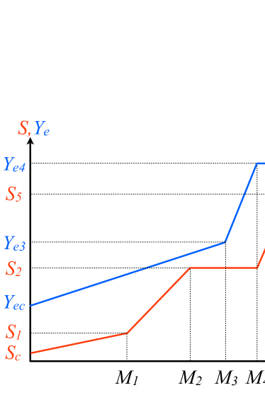
Figure 1: Schematic behavior of the entropy $S$ (red line) and electron fraction $Y_{e}$ (blue line) distribution as a function of mass for our progenitor models.

Following Baron & Cooperstein (1990) the entropy as a function of mass $M$ of our progenitor models is given by

$$S(M\leq M_{1}) =S_{c}+(S_{1}-S_{c})\left(\frac{M}{M_{1}}\right),$$ (2)

$$S(M_{1}\leq M\leq M_{2}) =S_{1}+(S_{2}-S_{1})\left(\frac{M-M_{1}}{M_{2}-M_{1}}\right),$$ (3)

$$S(M_{2}\leq M\leq M_{4}) =S_{2}=S_{3}=S_{4},$$ (4)

$$S(M_{4}\leq M\leq M_{5}) =S_{4}+(S_{5}-S_{4})\left(\frac{M-M_{4}}{M_{5}-M_{4}}\right),$$ (5)

$$S(M_{5}\leq M) =S_{5},$$ (6)

and the electron fraction by

$$Y_{e}(M\leq M_{3}) =Y_{ec}+(Y_{e3}-Y_{ec})\left(\frac{M}{M_{3}}\right),$$ (7)

$$Y_{e}(M_{3}\leq M\leq M_{4}) =Y_{e3}+(Y_{e4}-Y_{e3})\left(\frac{M-M_{c}}{M_{4}-M_{3}}\right),$$ (8)

$$Y_{e}(M_{4}\leq M) =Y_{e4},$$ (9)

(see also Fig. 1). These two distributions contain the parameters $M_{1}$, $M_{2}$, $M_{3}$, $M_{4}$, $M_{5}$, $S_{c}$, $S_{1}$, $S_{2}$, $S_{5}$, $Y_{ec}$, $Y_{e3}$, and $Y_{e4}$, which uniquely characterize the progenitor model.

The mass parameters have the following significance for an iron core which is undergoing silicon shell-burning after the central convective core has been exhausted of fuel. $M_{1}$ is the mass coordinate of the edge of the final convection in the radiative core, $M_{2}$ is the mass coordinate of the inner edge of the convection zone in the iron core, $M_{3}$ is the mass coordinate up to which the core matter is in nuclear statistical equilibrium (NSE core), $M_{4}$ is the iron core mass, and $M_{5}$ is the mass coordinate at the base of the silicon/oxygen shell which has a much larger entropy than the iron core ($S_{5}\gg S_{2}$) and consequently a much lower density.

Since the entropy distribution is a consequence of a complicated sequence of burning and convection stages, its profile is more structured than the $Y_{e}$ profile, because the latter only depends on the electron capture timescale. Different from Baron & Cooperstein (1990), we used two additional parameters, $M_{5}$ and $S_{5}$, in our study, because in more recent stellar evolutionary models the locations do not coincide where $S$ and $Y_{e}$ increase strongly. Also note that in Baron & Cooperstein (1990) the iron core mass is given by $(M_{3}+M_{4})/2$, whereas it is $M_{4}$ in our study.

According to stellar evolutionary calculations, these above parameters vary from progenitor model to progenitor model. For example, $S_{c}$ varies from $\sim 0.5$ to $\sim 2$, and the values of $M_{5}$ range from $\sim 1.2$ to $\sim 3.7$ (see Table 4 in the Appendix).

Table 1: Parameters of our models resembling the stellar evolutionary model s11.2 of Woosley et al. (2002)

Model	$M_{1}$	$M_{2}$	$M_{3}$	$M_{4}$	$M_{5}$	$S_{c}$	$S_{1}$	$S_{2}$	$S_{5}$	$Y_{ec}$	$Y_{e3}$	$Y_{e4}$	$\rho_{c}$	$g_{\mathrm{eff}}$
	[$M_{\odot}$]					[$k_{B}/$baryon]							[$10^{10}$g cm-3]
WHW02-s11.2-g0.99	0.82	1.16	1.26	1.30	1.32	0.62	1.1	1.74	5.4	0.425	0.48	0.5	1.6	0.99
WHW02-s11.2-g0.975	—	—	—	—	—	—	1.0	1.65	—	—	—	—	—	0.975
WHW02-s11.2-g0.95	—	—	—	—	—	—	0.75	1.64	—	—	—	—	—	0.95

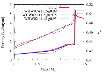
Figure 2: Entropy (solid) and electron fraction (dotted) distribution as a function of mass coordinate. Red lines give the distributions of the stellar evolutionary model s11.2 of Woosley et al. (2002), and the purple, blue, and green lines show the distributions of our models, whose parameters are given in Table 1.

Fig. 2 shows the $S$ (solid lines) and $Y_{e}$ (dotted lines) distributions of the three models investigated in this study (purple, blue, and green lines) compared to those of the stellar evolutionary model s11.2 (red line) of Woosley et al. (2002), which has been used in many core-collapse supernova studies during the past decade. In Table 1 we give the corresponding parameters of our three progenitor models, which have the same $Y_{e}$ profile, but differ by the values of $S_{1}$, $S_{2}$, and $g_{\mathrm{eff}}$. We used different values of $S_{1}$ and $S_{2}$ to match the density structure of the stellar evolutionary model s11.2, and varied the value of $g_{\mathrm{eff}}$ from 0.99 to 0.95. As shown in Fig. 3, all three models reproduce the density structure of model s11.2 very well.

2.3 Density structures

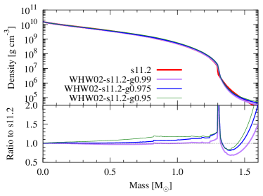
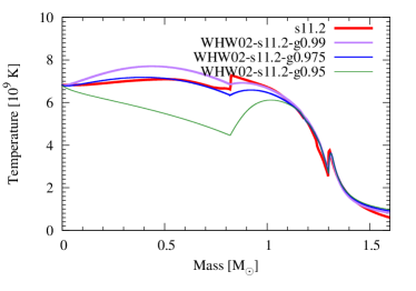
Figure 3: Density (top panel) and temperature (bottom panel) distributions of the stellar evolutionary model s11.2 (red) and of our three corresponding progenitor models (purple, blue, and green). The bottom plot in the upper panel shows the density distributions of our three models normalized by that of the s11.2 model.

The top panel of Fig. 3 shows the density structures of the stellar evolutionary model s11.2 together with those of our three corresponding progenitor models, which are obtained by integrating Eq. (1) numerically. The bottom plot of this panel, which displays the density distributions of our three models normalized by that of the s11.2 model, proves that our three models have almost the same density structure as model s11.2, the error being less than a few 10% except for the outermost layers ($M\mathrel{\hbox{\hbox to0.0pt{\hbox{\lower 5.0pt\hbox{$\sim$}}\hss}\hbox{$>$}}}1.3M_{\odot}$) of our models. On the other hand, the temperature structures (bottom panel in Fig. 3) of all of our three models differ significantly from that of model s11.2 for $M\mathrel{\hbox{\hbox to0.0pt{\hbox{\lower 5.0pt\hbox{$\sim$}}\hss}\hbox{$<$}}}1.0M_{\odot}$ because of they have quite different entropy profiles from the s11.2 model.

Obviously the parameterized progenitor models of Baron & Cooperstein (1990) can reproduce the progenitor structure of stellar evolutionary models at collapse considerably well. The model parameters that fit the structural properties of other progenitor models are given in Appendix A.

3 Hydrodynamic simulations

3.1 Method

For our simulations we used the code Agile-IDSA (Liebendörfer et al., 2009), which is a publicly available 1D neutrino-radiation hydrodynamics code for simulating core-collapse supernovae. The hydro solver, Agile (Adaptive Grid with Implicit Leap Extrapolation), integrates the general relativistic hydrodynamic equations in spherical symmetry (Liebendörfer et al., 2002), while the radiation transport part is an implementation of the isotropic diffusion source approximation (IDSA) (Liebendörfer et al., 2009), which has been used, e.g., by Suwa et al. (2010); Takiwaki et al. (2012); Nakamura et al. (2015), and Pan et al. (2016) to perform multi-dimensional core-collapse simulations. In IDSA the electron neutrino and electron anti-neutrino distribution functions are split into two components, which are solved with different numerical techniques.

The weak interaction rates implemented in our code are based on Mezzacappa & Bruenn (1993), and the cooling by muon and tau neutrinos is modeled with a leakage scheme. Neutrino-electron scattering is also implemented in this code according to Liebendörfer (2005) by expressing the electron fraction $Y_{e}$ as a function of $\rho$. However, since this function is calibrated for specific progenitor models and it is not always adequate, we did not employ it in this work. The equation of state (EOS) used in our simulations is that of Lattimer & Swesty (1991) with an incompressibility $K=220$ MeV for $\rho\geq 10^{8}$ g cm^-3 and that of Timmes & Arnett (1999) for $\rho<10^{8}$ g cm^-3. In the latter density range the average nuclear mass number $A$ and atomic number $Z$ are assumed to be the same as in the EOS of Lattimer & Swesty (1991) at $\rho=10^{8}$ g cm^-3. We follow O’Connor & Ott (2010) to match the thermodynamic quantities of both EOS tables at the transition density. The minimum density of of our combined EOS table is $10^{3}$ g cm^-3.

Accordingly, the results of our study are based on the use of a modern numerical tool that is well suited for simulations of neutrino-driven supernova explosions, because it is able to handle general relativistic gravity, neutrino radiation transport, and a nuclear equation of state. Nowadays we know that all of these ingredients are of considerable importance for a proper simulation of the supernova explosion mechanism, but none of them were taken into account in the work of Baron & Cooperstein (1990).

3.2 Results

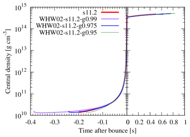
Figure 4: Central density as a function of time after bounce for the stellar evolutionary model s11.2 (red) and our three corresponding progenitor models (purple, blue, and green). The time of bounce differs, being later for models with a larger $g_{\mathrm{eff}}$ because these models are closer to a hydrostatic configuration.

Fig. 4 shows the central density as a function of time after bounce for all investigated models based on s11.2. Because our models were computed with different values of $g_{\mathrm{eff}}$, they bounce at different times, which range from $\sim 390$ to 170 ms. The density evolution of the stellar evolutionary model s11.2 is very similar to that of model WHW02-s11.2-g0.975 (although the central density of the model slightly decreases because the grid resolutions of the hydrodynamical simulations and those of the initial models differ). The figure implies that the collapse of our initially hydrostatic models with $g_{\mathrm{eff}}\mathrel{\hbox{\hbox to0.0pt{\hbox{\lower 5.0pt\hbox{$\sim$}}\hss}\hbox{$<$}}}0.975$ proceeds similarly to that of the already dynamically collapsing core of the stellar evolutionary progenitor model s11.2, even though the former models do not have any initial radial velocity.

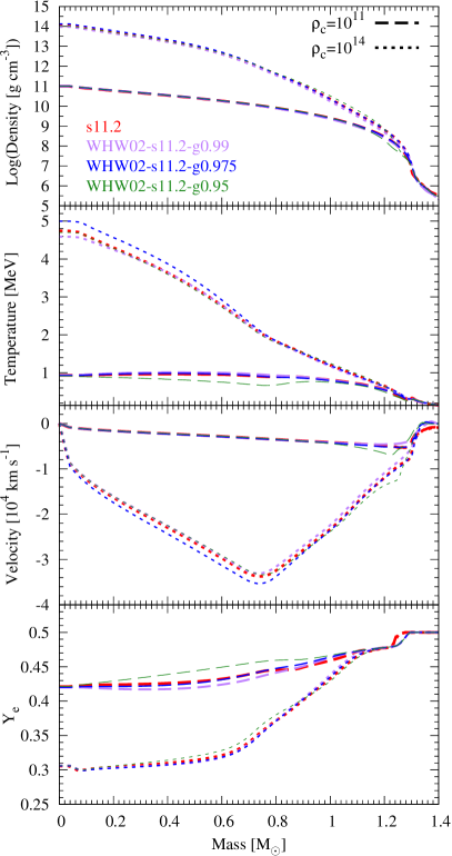
Figure 5: Comparison of the density, temperature, radial velocity, and electron fraction distributions (from top to bottom). Dashed and dotted lines give the profiles at the time when the central density reaches a value of about $10^{11}$ and $10^{14}$ g cm^-3, respectively.

Fig. 5 shows the evolution of the density, temperature, radial velocity, and electron fraction distributions before core bounce. The snapshots are taken at the time when the central density has a value of $\approx 10^{11}$ (dashed lines) and $\approx 10^{14}$ g cm^-3 (dotted lines), respectively. At the earlier snapshot ($\rho_{c}=10^{11}$ g cm^-3), the temperature distribution of model WHW02-s11.2-g0.95 is quite different, because its initial temperature profile differed significantly from those of all other models. At later times all models evolved quite similarly. The early electron fraction distributions exhibit larger difference than those of the other quantities, because the electron capture rate strongly depends on temperature ($\propto T^{6}$), i.e., a small difference in temperature can result in a large difference in $Y_{e}$. However, once $\beta-$equilibrium is achieved, the $Y_{e}$ distributions of the models become quite similar (see dotted lines in bottom panel).

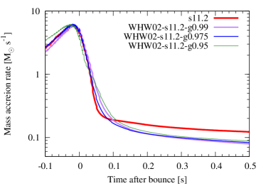
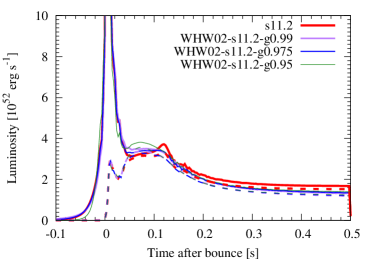
Figure 6: Evolution of the mass accretion rate (top) and of the electron neutrino (solid) and electron antineutrino (dashed) luminosities (bottom) of the stellar evolutionary model s11.2 (red) and our three corresponding progenitor models (purple, blue, and green).

In Fig. 6 we display the evolution of the mass accretion rate measured at a radius of 300 km (top panel) and of the electron neutrino (solid lines) and electron antineutrino (dashed lines) luminosities of the stellar evolutionary model s11.2 and of our three corresponding progenitor models. Because of small differences in the density structures of the models, both the mass accretion rates and the neutrino luminosities differ slightly between the models. About 50 ms post bounce, model s11.2 has the smallest mass accretion rate because the density gradient at $M\approx 1.3M_{\odot}$ is steepest for this model. At later times ($\sim 100$ ms post bounce) the mass accretion rate is largest in this model, because its density is the largest of all models in the relevant mass range $1.3\mathrel{\hbox{\hbox to0.0pt{\hbox{\lower 5.0pt\hbox{$\sim$}}\hss}\hbox{$<$}}}M/M_{\odot}\mathrel{\hbox{\hbox to0.0pt{\hbox{\lower 5.0pt\hbox{$\sim$}}\hss}\hbox{$<$}}}1.5$ (see Fig. 3).

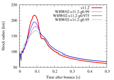
Figure 7: Shock trajectories for the stellar evolutionary model s11.2 (red) and our three corresponding progenitor models (purple, blue, and green).

Fig. 7 illustrates the shock evolution after core bounce. We define the shock position as the radius where the specific entropy reaches a value of $6\,k_{B}$ baryon^-1. Model s11.2 has the largest peak shock radius among all the investigated models, because it possesses the steepest density gradient (see Fig. 3). This fact leads to a rapid decrease of the mass accretion rate with radius and hence of the ram pressure on the shock. Since the shock radius is determined by the force balance between the thermal post-shock pressure and the pre-shock ram pressure, a lower ram pressure gives rise to a larger shock radius. Our three other corresponding progenitor models also show slightly different shock evolutions because their mass accretion rates differ from each other and from that of model s11.2 (see Fig. 6).

4 Parameter dependencies and explosion properties

Table 2: Parameters characterizing the entropy, electron fraction, and density distributions of our initial models, which all had $M_{1}=0.72M_{\odot}$, $M_{2}=1.0M_{\odot}$, $M_{3}=1.1M_{\odot}$, $M_{4}=1.15M_{\odot}$, $M_{5}=1.17M_{\odot}$, $Y_{e4}=0.5$, and $g_{\mathrm{eff}}=0.975$. The parameter values which differ from those of model BC01 are given in boldface.

Model	$S_{c}$	$S_{1}$	$S_{2}$	$S_{5}$	$Y_{ec}$	$Y_{e3}$	$\rho_{c}$
	[$k_{B}/$baryon]						[$10^{10}$ g cm-3]
BC01	0.5	0.63	1.6	4.0	0.415	0.46	2.0
BC02	0.4	0.63	1.6	4.0	0.415	0.46	2.0
BC03	0.6	0.63	1.6	4.0	0.415	0.46	2.0
BC04	0.5	0.53	1.6	4.0	0.415	0.46	2.0
BC05	0.5	0.73	1.6	4.0	0.415	0.46	2.0
BC06	0.5	0.63	1.5	4.0	0.415	0.46	2.0
BC07	0.5	0.63	1.7	4.0	0.415	0.46	2.0
BC08	0.5	0.63	1.6	3.0	0.415	0.46	2.0
BC09	0.5	0.63	1.6	6.0	0.415	0.46	2.0
BC10	0.5	0.63	1.6	4.0	0.411	0.46	2.0
BC11	0.5	0.63	1.6	4.0	0.425	0.46	2.0
BC12	0.5	0.63	1.6	4.0	0.415	0.452	2.0
BC13	0.5	0.63	1.6	4.0	0.415	0.47	2.0
BC14	0.5	0.63	1.6	4.0	0.415	0.46	1.0
BC15	0.5	0.63	1.6	4.0	0.415	0.46	3.0
BC16	0.4	0.73	1.6	4.0	0.415	0.46	2.0
BC17	0.4	0.63	1.7	4.0	0.415	0.46	2.0
BC18	0.4	0.63	1.6	6.0	0.415	0.46	2.0
BC19	0.4	0.63	1.6	4.0	0.425	0.46	2.0
BC20	0.4	0.63	1.6	4.0	0.415	0.47	2.0
BC21	0.4	0.63	1.6	4.0	0.415	0.46	1.0
BC22	0.4	0.63	1.6	4.0	0.415	0.46	3.0

In the last section, we demonstrated the reliability of the new method for constructing initial conditions for core-collapse supernova simulations by comparing models constructed by this method with a particular widely used presupernova model (WHW02-s11.2). The hydrodynamic features of these models agree with each other quite well. In Appendix A, we provide fitting parameters (see Table A1) which closely approximate the density structures of other presupernova models used in the literature (see Fig. 11).

Next we consider a second set of initial conditions differing from those reproducing progenitor models based on stellar evolutionary calculations. In particular, we present our numerical results for parameterized initial models based on model 109 of Baron & Cooperstein (1990), which has a relatively small central entropy and a small core mass, i.e. its structure differs significantly from that of initial models obtained with stellar evolutionary calculations. Thus, this second set of parametrized initial models allows us to study the dependence of the outcome of core-collapse supernova simulations for quite different initial conditions. The corresponding model parameters are given in Table 2.

We first changed the value of one parameter from model to model (BC01 to BC15 in Table 2), and then we fixed the value of the central entropy to $S_{c}=0.4$ and again changed one of the other parameters from model to model(BC16 to BC22 in Table 2). As we will show below, the reason for this approach was that model BC02 gives rise to a successful explosion, i.e., the parameter space around this model is worth investigating. We note that we restricted the parameters we chose in our study by the condition that the density at $M_{5}$ is larger than $10^{3}$ g cm^-3, which implies a lower limit for the entropy or the electron fraction, because a low entropy or electron fraction leads to a faster decrease of the density with increasing mass coordinate.

Table 3: Some properties characterizing our parametrized initial models

Model	$R(M_{5})^{a}$	$\rho(M_{5})^{b}$	$T(M_{5})^{c}$	${\xi_{M_{5}}}^{d}$	${\mu_{M_{5}}}^{e}$	${E_{b}}^{f}$
	[$10^{8}$ cm]	[$10^{6}$ g cm-3]	[$10^{9}$ K]			[B]
BC01	1.25	5.77	3.76	0.93	0.057	2.59
BC02	1.50	1.98	2.73	0.78	0.028	2.50
BC03	1.10	11.7	4.58	1.06	0.090	2.78
BC04	1.81	0.53	1.78	0.65	0.011	2.47
BC05	1.08	13.8	4.79	1.08	0.103	2.91
BC06	1.44	2.13	2.80	0.81	0.028	2.50
BC07	1.17	10.0	4.39	1.00	0.086	2.80
BC08	1.22	7.29	3.44	0.96	0.069	2.52
BC09	1.31	4.07	4.06	0.89	0.044	4.96
BC10	1.72	0.81	2.05	0.68	0.015	2.47
BC11	0.96	26.2	5.68	1.22	0.151	3.47
BC12	1.98	0.27	1.41	0.59	0.007	2.47
BC13	1.07	14.8	4.88	1.09	0.107	2.95
BC14	1.56	3.14	3.15	0.75	0.048	2.61
BC15	1.14	6.30	3.86	1.02	0.052	2.54
BC16	1.19	8.17	4.15	0.98	0.073	2.68
BC17	1.29	5.68	3.75	0.90	0.060	2.62
BC18	1.58	1.56	3.06	0.74	0.025	5.60
BC19	1.01	19.2	5.24	1.16	0.125	3.14
BC20	1.16	9.44	4.32	1.01	0.081	2.72
BC21	1.90	0.91	2.13	0.61	0.021	2.49
BC22	1.43	1.60	2.56	0.82	0.021	2.48

^a Radius of $M=M_{5}$

^b Density of $M=M_{5}$

^c Temperature of $M=M_{5}$

^d Compactness parameter, $\xi_{M}\equiv(M/M_{\odot})/[R(M)/1000~{}\mathrm{km}]$

^e $\mu_{M}\equiv dM/dR=4\pi R(M)^{2}\rho(M)$ in units of $M_{\odot}/1000$ km

^f Total binding energy

In Table 3 we give the values of some quantities characterizing the density structures of our second set of parametrized models. Columns 2 to 4 give the radius (in units of $10^{8}$ cm), the density (in units of $10^{6}$ g cm^-3), and the temperature (in units of $10^{9}$ K) at the mass coordinate $M=M_{5}$, respectively. In the fifth column we list the compactness parameter $\xi_{M}$ (O’Connor & Ott, 2011), which is defined as

$$\xi_{M}=\frac{M/M_{\odot}}{R(M)/1000\,\mathrm{km}},$$ (10)

where $R(M)$ is the radius of the sphere containing a mass $M$. Note that we use here the compactness parameter $\xi_{M_{5}}$, whereas O’Connor & Ott (2011) considered $\xi_{M=2.5M_{\odot}}$ instead. According to O’Connor & Ott (2011) smaller values of $\xi_{M}$ are better for explosions. Column 6 gives the parameter $\mu_{M}$, defined by Ertl et al. (2016) as

$$\mu_{M}=\left.\frac{dM}{dr}\right|_{r=R(M)}=4\pi\rho R^{2}(M).$$ (11)

Whereas Ertl et al. (2016) obtained the value of $dM/dr$ by computing the numerical derivative of $dM/dr$ at the mass shell where $S=4k_{B}$ baryon^-1 with a mass interval of $0.3M_{\odot}$, we used for simplicity the second equality in Eq. (11) to compute $dM/dr$ analytically. Ertl et al. (2016) showed that for a given value of $M_{S=4}$ (the mass coordinate where $S=4k_{B}$ baryon^-1), a smaller value of $\mu_{M}$ is better for an explosion. Finally, the last column gives the total binding energy of the initial model, which includes the contribution of the internal energy.

Figure 8: Model structure in a temperature-density plane. Black and grey lines give the profiles of our parameterized models and of models obtained from stellar evolutionary calculations (see Appendix A), respectively.

Fig. 8 shows the structure of our second set of parameterized models (solid lines) in a density-temperature plane. The additional grey lines give the structures of the models listed in Appendix A, which are obtained by stellar evolution calculations. Obviously, our parametrized models show a similar trend as the evolutionary ones, except for their non-monotonic behavior at densities $\rho\sim 10^{7}$ g cm^-3 and at densities of a few times $10^{9}$ g cm^-3, i.e. near the center. In other words, these models allow us to investigate thermodynamic regimes beyond those encountered in canonical models.

The Chandrasekhar mass is often used as a rough estimate of the iron core mass. Since the former mass depends on the electron fraction as

$$M_{ch} \approx 5.87Y_{e}^{2}M_{\odot}$$ (12)

$$=1.01\left(\frac{Y_{e}}{0.415}\right)^{2}M_{\odot},$$ (13)

our small iron core ($M_{4}=1.15M_{\odot}$) can be unstable.

Table 4: Overview of our hydrodynamic simulations

Model	${t_{\mathrm{bounce}}}^{a}$	${t_{400}}^{b}$	${t_{\mathrm{fin}}}^{c}$	${R_{\mathrm{shock,max}}}^{d}$	${M_{\mathrm{NS,final}}}^{e}$	${E_{\mathrm{diag,1000}}}^{f}$	${E_{\mathrm{diag,fin}}}^{g}$	${\dot{E}_{\mathrm{diag,fin}}}$h	${Y_{c,\mathrm{bounce}}}^{i}$	${E_{\mathrm{kin,init}}}^{j}$
	[ms]	[ms]	[ms]	[$10^{8}$ cm]	[$M_{\odot}$]	[B]	[B]	[B s-1]		[B]
BC01	252	—	944	0.244	1.22	—	—	—	0.328	7.81
BC02	254	21.9	452	2.908	1.09	0.145	0.294	3.8	0.336	8.44
BC03	245	—	981	0.203	1.27	—	—	—	0.319	7.09
BC04	248	—	841	0.274	1.19	—	—	—	0.327	7.80
BC05	255	—	928	0.209	1.28	—	—	—	0.328	7.71
BC06	242	—	1000	0.350	1.19	—	—	—	0.328	7.84
BC07	261	—	953	0.214	1.26	—	—	—	0.327	7.83
BC08	242	—	833	0.232	1.20	—	—	—	0.328	7.92
BC09	252	—	1000	0.312	1.26	—	—	—	0.327	7.76
BC10	249	—	855	0.316	1.18	—	—	—	0.327	7.65
BC11	249	—	1000	0.194	1.37	—	—	—	0.327	7.82
BC12	239	—	709	0.279	1.17	—	—	—	0.327	7.66
BC13	262	—	940	0.205	1.29	—	—	—	0.328	8.00
BC14	401	—	997	0.248	1.21	—	—	—	0.327	7.68
BC15	189	—	733	0.259	1.21	—	—	—	0.327	7.84
BC16	259	—	1000	0.283	1.25	—	—	—	0.335	8.44
BC17	263	23.8	496	2.487	1.10	0.160	0.331	3.4	0.336	8.39
BC18	259	21.2	451	3.000	1.08	0.132	0.386	4.7	0.336	8.50
BC19	254	—	1000	0.873	1.32	—	—	—	0.340	9.50
BC20	267	—	1000	0.542	1.26	—	—	—	0.336	8.51
BC21	397	22.5	590	3.120	1.09	0.090	0.269	4.1	0.336	8.45
BC22	192	22.2	392	3.060	1.08	0.141	0.234	2.9	0.336	8.48

^a Time until bounce since the beginning of the simulation

^b Time past bounce when the shock reaches a radius of 400 km in the exploding models

^c Final time of the simulation

^d Maximum shock radius

^e Final mass of the PNS, which is defined by $\rho>10^{11}$ g cm^-3

^f Diagnostic explosion energy when the shock reaches a radius of 1000 km

^g Diagnostic explosion energy at $t_{\mathrm{fin}}$, when it is still increasing

^h Growth rate of the diagnostic explosion energy estimated 30 ms before $t_{\mathrm{fin}}$

ⁱ Value of $Y_{e}$ in the center at $t_{\mathrm{bounce}}$

^j Initial kinetic energy, which is estimated by the maximum value of the kinetic energy inside the mass of the largest infall velocity

Figure 9: Evolution of the diagnostic explosion energy for model BC18.

In Table 4 we provide an overview of the hydrodynamic simulations with our second set of models. The table columns give the time until bounce, the postbounce time when the shock reaches a radius of 400 km, the final time of the simulation, the maximum shock radius, the final baryonic mass of the PNS, and the diagnostic explosion energy at the times when the shock reaches a radius of 1000km and at ${t_{\mathrm{fin}}}$, respectively. The growth rate of the diagnostic energy at ${t_{\mathrm{fin}}}$ is given in the next column. The remaining columns give the value of $Y_{e}$ in the center at $t_{\mathrm{bounce}}$, and the initial kinetic energy. The PNS mass is defined as the mass with $\rho>10^{11}$ g cm^-3, and the diagnostic explosion energy as the integral of the local energy, i.e. the sum of the specific internal, kinetic and gravitational energies, of all zones where this quantity and the radial velocity are positive. Here we used the general relativistic expression for the local energy of Müller et al. (2012), which is given as

$$e_{\mathrm{local}}=\alpha\left[\left(\rho c^{2}+\epsilon c^{2}+P\right)W^{2}-P\right]-\rho Wc^{2},$$ (14)

where $\alpha$ is the lapse function, $c$ the speed of light, $\epsilon$ the specific internal energy, and $W$ the Lorentz factor. This expression reduces to the well-known Newtonian expression ($e_{\mathrm{local}}=\rho\phi+\rho v^{2}/2+\rho\epsilon$ with $\phi$ and $v$ being the gravitational potential and the velocity, respectively) when one omits higher-order terms like $(v/c)^{2}$.

Figure 10: Score sheet providing an overview (in the $S_{c}$-$S_{5}$ plane) of the models exploding or failing. Exploding models are marked by open circles and non-exploding oners are represented by crosses. The size of the circle is proportional to the growth rate of the diagnostic explosion energy (see Table 4). The numbers attached to the symbols give the number of non-exploding models with $\rho_{c}=2\times 10^{9}$ g cm^-3.

For model BC18, which produces the most energetic explosion of our second set of models, $S_{c}=0.4$ and $S_{5}=6\,k_{B}$ baryon^-1. The diagnostic explosion energy of this model already reaches 0.39 B (= $3.9\times 10^{50}$ erg) at the end of the simulation, and it is still increasing (see Fig. 9) at a rate of $\approx$4.7 B s^-1, i.e., it will reach a value of 1 B about 320 ms after core bounce. Figure 10 presents a score sheet, which provides an overview (in the $S_{c}$-$S_{5}$ plane) of the models exploding or failing. The exploding models are marked by open circles, while the non-exploding models are represented by crosses. The size of the circles is proportional to the growth rate of the diagnostic explosion energy towards the end of the simulation (see Table 4). Obviously, smaller values of $S_{c}$ lead to a larger diagnostic explosion energy, and larger values of $S_{5}$ give rise to a faster growth rate of the diagnostic explosion energy in case of the exploding models.

Concerning the explosion energy one should note that the envelope located above the Si/O layer has a large binding energy of $O(10^{49})$ to $O(10^{51})$, the actual value depending on the ZAMS mass of the progenitor (e.g. Pejcha & Thompson, 2015). Therefore, the values given in Table 4 are not the observable explosion energies. To determine the latter energies, one needs to perform long-term simulations including the stellar envelopes, which will be left for future work.

For our second set of models, the electron fraction at bounce is larger than in the simulations with our first set of models based on the stellar evolutionary model s11.2 (see previous section and Fig. 5), in which $Y_{c,\mathrm{bounce}}\approx 0.3$. Because of their smaller initial central entropy, the latter models have a lower temperature, which implies a smaller electron capture rate during collapse. The resulting larger electron fractions explain the larger kinetic energies at the bounce (see, e.g. Müller, 1998), which are given by the kinetic energy of the inner core at the “last good homology” (Brown et al., 1982). Of the models listed in the upper part of Table 4, model BC02 has the largest initial kinetic energy. Among these models, model BC02 is also the only exploding model. Although a higher value of $Y_{ec}$ also leads to a larger value of $Y_{c,\mathrm{bounce}}$ and a larger initial kinetic energy (see model BC19 in the lower part of Table 4), model BC19 does not explode because of its larger gravitational binding energy (see Table 3). However, we note that in comparison to the other non-exploding models (BC16-BC18, BC20-BC22), the shock propagates out to an exceptionally large maximum shock radius of 873 km in model BC19, i.e, it is a marginal model marking the boundary between exploding and non-exploding models.

In all exploding models the explosion sets in early ($\sim$ 20 ms after core bounce), which seems to suggest a prompt explosion. However, these explosions are still aided by neutrino heating, i.e., they differ from prompt explosion models, in which initial kinetic energy is large enough to eject the envelope. To validate this statement, we performed a simulation without neutrino heating by setting the distribution function of streaming particles, which is essential for neutrino heating in IDSA (see Liebendörfer et al., 2009), to zero. Then, the exploding model does no longer explode, i.e., it was no prompt explosion.

From these result, we conclude that the iron core structure is crucial for obtaining an explosion. Especially, a low entropy at the center helps to make an explosion. To reach a more general conclusion, we need a large number of simulations covering a wider range of parameter space, which will be reported in a forthcoming publication.

5 Summary and discussion

In this paper, we investigated a method to construct parametrized initial progenitor models for core-collapse supernova simulations. So far, initial conditions of these simulations have been taken from the final phase of stellar evolutionary calculations, which depend on several uncertainties, like the treatments of semi-convection, overshooting, and composition mixing. In particular, many phenomenological treatments are employed to approximate multi-dimensional effects in evolution simulations done in spherical symmetry. In this paper, we proposed a alternative methodology to construct initial conditions. This is not a completely new idea and we reused a method by Baron & Cooperstein (1990). However, different from these authors, we used the latest input microphysics including neutrino transfer, a microscopic nuclear equation of state and general relativistic hydrodynamics. In their paper, they presented functions of entropy and electron fraction expressed by mass coordinate. With these functions and solving hydrostatic equation, we can construct initial density structures.

First of all, we constructed structures with parameters fitting the commonly used model s11.2 from Woosley et al. (2002) and showed the similarity between our models and the model s11.2. We then performed general relativistic neutrino-radiation hydrodynamics simulations in spherical symmetry with the public code Agile-IDSA (Liebendörfer et al., 2009) and showed the reliability of our method. Next, we constructed models based on parameters given in Baron & Cooperstein (1990) and studied parameter dependencies. Interestingly, we found several exploding models with small central entropy even in spherically symmetric simulations. More surprisingly, models with a large entropy in the Si/O layer give rather large explosion energies, $\sim 4\times 10^{50}$ erg at the final time of our simulations, and the energy still being increasing.

Nevertheless of the large explosion energy ($\mathrel{\hbox{\hbox to0.0pt{\hbox{\lower 5.0pt\hbox{$\sim$}}\hss}\hbox{$>$}}}4\times 10^{50}$ erg), we find that the PNS masses are rather small ($\sim 1.1M_{\odot}$ in baryonic mass) for exploding models, so that these explosions are not fully compatible with observations. This discrepancies will be reduced when we use multi-dimensional simulations, since multi-dimensional effects amplify neutrino heating and explodability significantly. These simulations would produce an explosion for models that do not explode in spherically-symmetric simulations for a larger value of the central entropy, and would lead to continuous mass accretion onto a PNS. With multi-D simulations, we may find parameter sets leading to a large explosion energy, $\sim 10^{51}$ erg, and a typical NS gravitational mass, $\sim$ 1.3–2.0 $M_{\odot}$, which is typically $\sim 10$% smaller than the baryonic mass. A broader parameter survey is necessary to explore these more promising combinations.

In this study we considered initial modesl with different entropy stratificationss, but did not pay much attention to the temperature profiles. However, the temperature distribution is crucially important for nuclear synthesis and the energy generation rate in burning layers. Therefore, our current model might not be fully consistent with stellar evolution and an improvement will be presented in the forthcoming papers.

This work is the very first step toward investigating initial conditions other than those resulting from stellar evolutionary calculations. The virtue of the method used in our study is that we can choose initial conditions beyond those predicted by current stellar evolutionary calculations. Hence, we may be able to find robust conditions for energetic explosions, i.e. explosions in which the energy is larger than the canonical value $10^{51}$ erg. This is one of the important goals for the core-collapse supernova simulation community.

Appendix A Fitting other progenitor models

In the main text, we discussed a set of models based on the stellar evolutionary model s11.2 of Woosley et al. (2002), since it is a well studied model in the literature. In this appendix, we give the fitting parameters (Table 5) and density structures (Fig. 11) of parameterized models reproducing other typical progenitor models for convenience.

Table 5: Parameters for a set of stellar evolutionary models

Model	$M_{1}$	$M_{2}$	$M_{3}$	$M_{4}$	$M_{5}$	$S_{c}$	$S_{1}$	$S_{2}$	$S_{5}$	$Y_{ec}$	$Y_{e3}$	$Y_{e4}$	$\rho_{c}$	$g_{\mathrm{eff}}$
	[$M_{\odot}$]					[$k_{B}/$baryon]							[$10^{10}$g cm-3]
Parameterized models fitting models s15.0 and s40.0 of Woosley et al. (2002)
WHW02-s15.0	1.05	1.3	1.3	1.6	1.84	0.75	1.5	2.7	4.5	0.437	0.472	0.5	0.63	0.975
WHW02-s40.0	0.98	1.55	1.55	1.84	1.86	0.96	1.6	2.6	5.8	0.443	0.48	0.5	0.37	0.975
Parameterized model fitting model 8.8$M_{\odot}$ (O-Ne-Mg core) of Nomoto (1984, 1987)
N87-ONeMg	—	—	0.63	0.72	—	0.55	0.55	0.55	0.55	0.488	0.488	0.5	3.0	0.99
Parameterized models fitting models N13 and N15 of Nomoto & Hashimoto (1988)
NH88-N13	0.68	1.11	1.15	1.17	1.18	0.65	0.97	1.54	4.2	0.406	0.462	0.5	3.0	0.975
NH88-N15	0.7	1.2	1.3	1.31	1.38	0.74	1.01	2.26	5.0	0.411	0.472	0.5	3.1	0.975
Parameterized models fitting models s12, s15, s20, and s25 of Woosley & Heger (2007)
WH07-s12	0.95	1.2	1.26	1.3	1.32	0.7	1.1	2.2	3.5	0.43	0.48	0.5	1.2	0.975
WH07-s15	1.0	1.3	1.34	1.35	1.42	0.78	1.4	2.2	3.7	0.436	0.48	0.5	0.72	0.975
WH07-s20	0.96	1.5	1.54	1.81	1.82	0.93	1.56	2.62	5.0	0.443	0.482	0.5	0.36	0.975
WH07-s25	0.96	1.58	1.58	1.89	1.9	0.93	1.56	2.9	5.0	0.444	0.482	0.5	0.34	0.975
Parameterized model fitting model 15$M_{\odot}$ of Limongi & Chieffi (2006)
LC06-m15	1.12	1.38	1.38	1.6	1.78	0.66	1.5	2.7	5.0	0.454	0.48	0.5	0.52	0.975
Parameterized models fitting models s15s7b2, s25s7b8, and s40s7b2 of Woosley & Weaver (1995)
WW95-s15s7b2	0.95	1.28	1.28	1.42	1.43	0.7	1.3	2.1	4.5	0.432	0.476	0.5	1.0	0.975
WW95-s25s7b8	1.07	1.35	1.72	2.05	2.06	1.0	1.7	2.75	5.5	0.448	0.484	0.5	0.26	0.975
WW95-s40s7b2	1.24	1.88	1.88	3.2	3.7	1.15	2.0	4.24	6.6	0.448	0.49	0.5	0.23	0.975
Parameterized model fitting model CO15 of Suwa et al. (2015)
SYSUT15-CO15	1.0	1.1	1.11	1.3	1.42	0.65	1.25	1.9	4.7	0.43	0.468	0.5	1.0	0.99

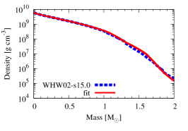
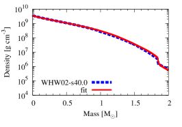
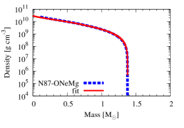
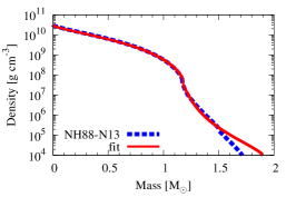
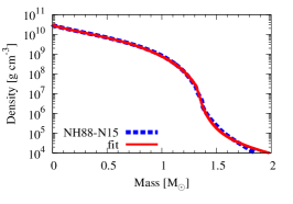
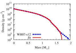
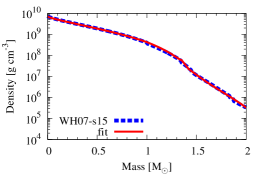
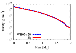
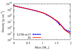
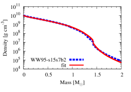
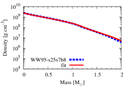
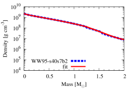
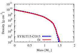
Figure 11: Density structures of various stellar evolutionary progenitor models (blue dashed lines) and parameterized models fitting these models (red solid lines). The corresponding parameters are given in Table 5.

References

- Arnett & Meakin (2011) Arnett W. D., Meakin C., 2011, ApJ, 733, 78
- Baron & Cooperstein (1990) Baron E., Cooperstein J., 1990, ApJ, 353, 597
- Brown et al. (1982) Brown G. E., Bethe H. A., Baym G., 1982, Nuclear Physics A, 375, 481
- Bruenn et al. (2013) Bruenn S. W., Mezzacappa A., Hix W. R., et al., 2013, ApJ, 767, L6
- Buras et al. (2006) Buras R., Janka H., Rampp M., Kifonidis K., 2006, A&A, 457, 281
- Burrows (2013) Burrows A., 2013, Reviews of Modern Physics, 85, 245
- Burrows et al. (2006) Burrows A., Livne E., Dessart L., Ott C. D., Murphy J., 2006, ApJ, 640, 878
- Couch et al. (2015) Couch S. M., Chatzopoulos E., Arnett W. D., Timmes F. X., 2015, ApJ, 808, L21
- Couch & Ott (2013) Couch S. M., Ott C. D., 2013, ApJ, 778, L7
- Dolence et al. (2015) Dolence J. C., Burrows A., Zhang W., 2015, ApJ, 800, 10
- Ertl et al. (2016) Ertl T., Janka H.-T., Woosley S. E., Sukhbold T., Ugliano M., 2016, ApJ, 818, 124
- Foglizzo et al. (2015) Foglizzo T., Kazeroni R., Guilet J., et al., 2015, Publ. Astron. Soc. Australia, 32, 9
- Hanke et al. (2013) Hanke F., Müller B., Wongwathanarat A., Marek A., Janka H.-T., 2013, ApJ, 770, 66
- Janka (2012) Janka H.-T., 2012, Annual Review of Nuclear and Particle Science, 62, 407
- Jones et al. (2015) Jones S., Hirschi R., Pignatari M., et al., 2015, MNRAS, 447, 3115
- Kotake et al. (2012) Kotake K., Takiwaki T., Suwa Y., et al., 2012, Advances in Astronomy, 2012, 39
- Lattimer & Swesty (1991) Lattimer J. M., Swesty F. D., 1991, Nuclear Physics A, 535, 331
- Lentz et al. (2015) Lentz E. J., Bruenn S. W., Hix W. R., et al., 2015, ApJ, 807, L31
- Liebendörfer (2005) Liebendörfer M., 2005, ApJ, 633, 1042
- Liebendörfer et al. (2002) Liebendörfer M., Rosswog S., Thielemann F.-K., 2002, ApJS, 141, 229
- Liebendörfer et al. (2009) Liebendörfer M., Whitehouse S. C., Fischer T., 2009, ApJ, 698, 1174
- Limongi & Chieffi (2006) Limongi M., Chieffi A., 2006, ApJ, 647, 483
- Marek & Janka (2009) Marek A., Janka H., 2009, ApJ, 694, 664
- Meakin & Arnett (2007) Meakin C. A., Arnett D., 2007, ApJ, 667, 448
- Melson et al. (2015) Melson T., Janka H.-T., Marek A., 2015, ApJ, 801, L24
- Mezzacappa & Bruenn (1993) Mezzacappa A., Bruenn S. W., 1993, ApJ, 405, 669
- Müller (2015) Müller B., 2015, MNRAS, 453, 287
- Müller & Janka (2015) Müller B., Janka H.-T., 2015, MNRAS, 448, 2141
- Müller et al. (2012) Müller B., Janka H.-T., Marek A., 2012, ApJ, 756, 84
- Müller (1998) Müller E., 1998, in Saas-Fee Advanced Course 27: Computational Methods for Astrophysical Fluid Flow., edited by O. Steiner, A. Gautschy, 343
- Nakamura et al. (2015) Nakamura K., Takiwaki T., Kuroda T., Kotake K., 2015, PASJ, 67, 107
- Nomoto (1984) Nomoto K., 1984, ApJ, 277, 791
- Nomoto (1987) Nomoto K., 1987, ApJ, 322, 206
- Nomoto & Hashimoto (1988) Nomoto K., Hashimoto M., 1988, Phys. Rep., 163, 13
- O’Connor & Couch (2015) O’Connor, E., & Couch, S. 2015, arXiv:1511.07443
- O’Connor & Ott (2010) O’Connor E., Ott C. D., 2010, Classical and Quantum Gravity, 27, 11, 114103
- O’Connor & Ott (2011) O’Connor E., Ott C. D., 2011, ApJ, 730, 70
- O’Connor & Ott (2013) O’Connor E., Ott C. D., 2013, ApJ, 762, 126
- Ott et al. (2008) Ott C. D., Burrows A., Dessart L., Livne E., 2008, ApJ, 685, 1069
- Pan et al. (2016) Pan K.-C., Liebendörfer M., Hempel M., Thielemann F.-K., 2016, ApJ, 817, 72
- Pejcha & Thompson (2015) Pejcha O., Thompson T. A., 2015, ApJ, 801, 90
- Sukhbold et al. (2015) Sukhbold, T., Ertl, T., Woosley, S. E., Brown, J. M., & Janka, H.-T. 2015, arXiv:1510.04643
- Suwa et al. (2010) Suwa Y., Kotake K., Takiwaki T., Whitehouse S. C., Liebendörfer M., Sato K., 2010, PASJ, 62, L49
- Suwa et al. (2016) Suwa Y., Yamada S., Takiwaki T., Kotake K., 2016, ApJ, 816, 43
- Suwa et al. (2015) Suwa Y., Yoshida T., Shibata M., Umeda H., Takahashi K., 2015, MNRAS, 454, 3073
- Takiwaki et al. (2012) Takiwaki T., Kotake K., Suwa Y., 2012, ApJ, 749, 98
- Timmes & Arnett (1999) Timmes F. X., Arnett D., 1999, ApJS, 125, 277
- Ugliano et al. (2012) Ugliano M., Janka H.-T., Marek A., Arcones A., 2012, ApJ, 757, 69
- Woosley & Heger (2007) Woosley S. E., Heger A., 2007, Phys. Rep., 442, 269
- Woosley et al. (2002) Woosley S. E., Heger A., Weaver T. A., 2002, Reviews of Modern Physics, 74, 1015
- Woosley & Weaver (1995) Woosley S. E., Weaver T. A., 1995, ApJS, 101, 181
- Yamamoto & Yamada (2016) Yamamoto Y., Yamada S., 2016, ApJ, 818, 165