Conditions for observing emergent SU(4) symmetry in a double quantum dot

Abstract

We analyze conditions for the observation of a low energy SU(4) fixed point in capacitively coupled quantum dots. One problem, due to dots with different couplings to their baths, has been considered by Tosi, Roura-Bas and Aligia (2015). They showed how symmetry can be effectively restored via the adjustment of individual gates voltages, but they make the assumption of infinite on-dot and inter-dot interaction strengths. A related problem is the difference in the magnitudes between the on-dot and interdot strengths for capacitively coupled quantum dots. Here we examine both factors, based on a two site Anderson model, using the numerical renormalization group to calculate the local spectral densities on the dots and the renormalized parameters that specify the low energy fixed point. Our results support the conclusions of Tosi et al. that low energy SU(4) symmetry can be restored, but asymptotically achieved only if the inter-dot interaction $U_{12}$ is greater than or of the order of the band width of the coupled conduction bath $D$, which might be difficult to achieve experimentally. By comparing the SU(4) Kondo results for a total dot occupation $n_{\rm tot}=1$ and $n_{\rm tot}=2$ we conclude that the temperature dependence of the conductance is largely determined by the constraints of the Friedel sum rule rather than the SU(4) symmetry and suggest that an initial increase of the conductance with temperature is a distinguishing characteristic feature of an $n_{\rm tot}=1$ universal SU(4) fixed point.

I Introduction

Quantum dots have proved to be ideal systems for studying the low energy behavior of strongly correlated local systems as described by single impurity Anderson and Kondo models. This is because the energy levels on the dots and their connections to a host electron bath can be controlled and manipulated by applied gate voltages. This has enabled the Kondo effect, arising from the SU(2) spin degeneracy in a single quantum dot, to be probed experimentally. Measurements of the current flow through the dot, due to an applied bias voltage, have revealed in detail the many-body low temperature induced resonance in the local density of states in the Kondo regimeGoldhaber-Gordon et al. (1998); Cronenwett et al. (1998); van der Wiel et al. (2000); Kogan et al. (2004); Amasha et al. (2005). Interest has naturally moved on to the observation of other types of strong correlation states.

There have been several theoretical papers dealing with the possibility of observing an SU(4) Kondo state in a capacitively coupled double quantum dot Borda et al. (2003); Mitchell et al. (2006); Tosi et al. (2013); Nishikawa et al. (2013); Filippone et al. (2014); Bau et al. (2014); Tosi et al. (2015). In this arrangement an SU(2) pseudospin symmetry is introduced in addition to the SU(2) spin symmetry by using two identical quantum dots with a total occupation number for the double dot maintained such that $n_{\rm tot}=1$. The occupation of dot 1 then corresponds to an ’up’ pseudospin and the occupation number for the second dot 2 as pseudospin ’down’. One motivation for such an arrangement is that it allows one to measure ’spin’ polarized currents without the need to introduce a local magnetic field Büsser et al. (2012).

Recent experimental workHübel et al. (2008); Amasha et al. (2013) in which the electron transport through the individual dots has been measured for such a system, has revealed directly the effects of the pseudospin degrees of freedom, and provided some support for the interpretation as arising from an SU(4) fixed point Keller et al. (2014).

In our earlier work Nishikawa et al. (2013) on this topic we used the numerical renormalization group (NRG) to calculate the renormalized parameters which specify the effective Hamiltonian which determines the low energy behavior of the system. This led us to the conclusion that it would be difficult to observe complete SU(4) low energy fixed point behavior due to the smaller inter-dot interaction compared with the on-dot term. Here we expand upon that work to get some estimates as to whether an SU(4) fixed point can be realized, given experimentally accessible ranges for the inter-dot and on-dot interactions, $U_{12}$ and $U$, respectively. We can check, in the case that it is not completely realized, how close the low temperature behavior is to such a fixed point. By comparing the full spectral density on the dots with that derived in terms of the low energy quasiparticles we can also test the range of the low energy effective theory. There can also be a potential problem, considered by Tosi, Roura-Bas and Aligia Tosi et al. (2015), arising from a lack of symmetry due to from different couplings between the baths and their respective dots. They showed, however, that when both $U_{12}$ and $U$ are taken as infinitely large, this symmetry can be restored by appropriately adjusting the gate voltages to each dot. Here we test whether or not their conclusion holds for finite strength interactions $U_{12}$ and $U$.

To get a clearer understanding of the physics in the strong correlation regime we compare the SU(4) system with $n_{\rm tot}=1$, which is due to a combination of spin and pseudospin, with that for $n_{\rm tot}=2$, which is due to spin alone. We estimate and compare the leading temperature corrections to the zero bias conductances through the individual dots in the two cases. We conclude that temperature dependence of the conductances reflect the general features of the quasiparticle spectra rather than any strict symmetry conditions at the low energy fixed point.

II Double-Dot Model

The capacitively coupled quantum dot system can be described by a two site Anderson model of the form,

$$H=\sum_{i=1,2}(H_{i}+H_{{\rm bath},i}+H_{{\rm c},i})+H_{12},$$ (1)

where $H_{i}$ describes the individual dots, $i=1,2$, $H_{{\rm bath},i}$ the baths to which the dots are individually coupled by a term $H_{{\rm c},i}$, and $H_{12}$ is the interaction between the dots. A reasonable approximation is to take the baths, two for each dot, to be described by a free electron model,

$$H_{{\rm bath},i}=\sum_{{\bf k},\alpha,{\sigma}}\varepsilon_{\bf k}c^{\dagger}_{{\bf k},i,\alpha,\sigma}c_{{\bf k},i,\alpha,\sigma}$$ (2)

where $\alpha=s,d$ (source, drain) and $\varepsilon_{\bf k}$ is an energy level in a bath, taken to be independent of $\alpha$, $i$ and $\sigma$.

The Hamiltonian describing the dots $H_{i}$ is taken in the form,

$$H_{i}=\sum_{{\sigma}}\varepsilon_{i,\sigma}d^{\dagger}_{i,\sigma}d_{i,\sigma}+U_{i}n_{i,\uparrow}n_{i,\downarrow},$$ (3)

where $\varepsilon_{i,\sigma}$ is the level position on dot $i$, $\varepsilon_{i,\sigma}=\varepsilon_{i}$, relative to the chemical potential $\mu_{i}$, and $U_{i}$ is the intra-dot interaction.

The coupling of the dots to the leads is described by a hybridization term,

$$H_{{\rm c},i}=\sum_{{\bf k},\alpha,i,{\sigma}}V_{{\bf k},\alpha,i}(c^{\dagger}_{{\bf k},i,\alpha,\sigma}d_{i,\sigma}+\mathrm{h.c.}).$$ (4)

We will assume no energy dependence of the matrix elements but allow them to differ in the different channels. We define the widths $\Gamma_{i}=\sum_{\alpha}\pi V_{\alpha,i}^{2}\rho_{c}(0)$, where $\rho_{c}(0)$ is the conduction electron density of states at the Fermi level, as the constant energy scale for the hybridization. For transport close to equilibrium only the combination $V_{i,s}c^{\dagger}_{{\bf k},i,s,\sigma}+V_{i,d}c^{\dagger}_{{\bf k},i,d,\sigma}$ couples to the dot states. We can therefore simplify the problem to two dots and two itinerant channels.

Finally for capacitively coupled dots we assume a repulsive interaction term between the charges on the individual dots $U_{12}$,

$$H_{12}=U_{12}\sum_{\sigma,\sigma^{\prime}}n_{1,\sigma}n_{2,\sigma^{\prime}}.$$ (5)

If the dots are identical, with equal coupling to their baths and $U_{12}=U$, then the model has SU(4) symmetry. This can be shown explicitly by combining the site and spin indices, $(i,\sigma)\to\nu=((-1)^{i}+5/2+\sigma)$, where $\sigma=\pm 1/2$, so $\nu=1,2,3,4$, and express the Hamiltonian in terms of the creation and annihilation operators $c^{\dagger}_{\nu}$ and $c_{\nu}$. In the regimes with integral total occupation number $n_{\rm tot}=1,2,3$, which requires strong local interactions, this SU(4) Anderson model can be mapped into an SU(4) Kondo model,

$${\cal H}_{\rm K}=J\sum_{\nu,\nu^{\prime},k,k^{\prime}}Y_{\nu,\nu^{\prime}}c^{\dagger}_{k^{\prime},\nu^{\prime}}c_{k,\nu}+\sum_{\nu,k}\varepsilon_{k}c^{\dagger}_{k,\nu}c_{k,\nu},$$ (6)

where the sum over $\nu=1,2,...4$, and for $U>D$, $J=4|V|^{2}/U$ in the case with particle-hole symmetry. The operators $Y_{\nu,\nu^{\prime}}$ obey the SU(2n) commutation relations,

$$[Y_{\nu,\nu^{\prime}},Y_{\nu^{\prime\prime},\nu^{\prime\prime\prime}}]_{-}=Y_{\nu,\nu^{\prime\prime\prime}}\delta_{\nu^{\prime},\nu^{\prime\prime}}-Y_{\nu^{\prime\prime},\nu^{\prime}}\delta_{\nu,\nu^{\prime\prime\prime}},$$ (7)

with $\sum_{\nu}Y_{\nu,\nu}=nI$, where $I$ is the identity operator. The case with $n_{\rm tot}=1$ corresponds to the situation where the occupation of the individual dots plays the role of a pseudospin, and the $Y_{\nu,\nu^{\prime}}$ operators correspond to the four dimensional (fundamental) representation of SU(4). It is also a particular case of the model introduced by Coqblin and Schrieffer Coqblin and Schrieffer (1969) to describe certain rare earth magnetic impurities (similarly for the case $n_{\rm tot}=3$ in terms of holes). However, for the Kondo model with integral occupation on each dot, such that $n_{\rm tot}=2$, the operators correspond to a six dimensional irreducible representation of SU(4) Nishikawa et al. (2010).

For two capacitively coupled dots there is no symmetry or constraint such that $U_{12}=U$, so we expect the on-site interaction $U$ to be significantly greater than the inter-site interaction $U_{12}$. Estimates of the magnitude of the different interaction terms have been given in recent experimental work Amasha et al. (2013): $U_{1}\approx 1.2$meV, $U_{2}\approx 1.5$meV, $U_{12}\approx 0.1$meV, $\Gamma_{1},\Gamma_{2}\approx 0.005-0.02$meV, so realistically there is no SU(4) symmetry in the ’bare’ model. We are concerned with the low energy regime, however, where the effective or renormalized interactions determine the behavior. There is the possibility that a new SU(4) symmetry can emerge on this scale, as originally predicted on the basis of scaling equations from the high energy regime by Borda et al.Borda et al. (2003). In the next section we derive precise criteria for a low energy SU(4) fixed point in terms of renormalized parameters.

III Renormalized Parameters

We start from an exact expression for the Fourier transform of the one-electron Green’s function $G_{i}(\omega)$ for dot $i$,

$$G_{i}(\omega)=\frac{1}{\omega-\varepsilon_{i}+i\Gamma_{i}-\Sigma_{i}(\omega)},$$ (8)

where $\Sigma_{i}(\omega)$ is the proper self-energy. The corresponding spectral density $\rho_{i}(\omega)$ is

$$\rho_{i}(\omega)=-\frac{1}{\pi}\lim_{\delta\to 0}{\rm Im}\,G_{i}(\omega+i\delta)=\quad\quad\quad\quad$$

$$\frac{1}{\pi}\frac{\Gamma_{i}-\Sigma^{I}_{i}(\omega)}{(\omega-\varepsilon_{i}-\Sigma^{R}_{i}(\omega))^{2}+(\Gamma_{i}-\Sigma^{I}_{i}(\omega))^{2}},$$ (9)

where $\Sigma^{R}_{i}(\omega)$ and $\Sigma^{I}_{i}(\omega)$ are the real and imaginary parts of the self-energy. We assume that the low energy behavior corresponds to a Fermi liquid so that $\Sigma^{I}_{i}(\omega)$ is of order $\omega^{2}$ as $\omega\to 0$. We can define a set of renormalized parameters Hewson (1993); Hewson et al. (2004), $\tilde{\varepsilon}_{i}$, $\tilde{\Gamma}_{i}$, $\tilde{U}_{i}$ and $\tilde{U}_{12}$,

$$\tilde{\varepsilon}_{i}=z_{i}(\varepsilon_{i}+\Sigma(0)),\quad\tilde{\Gamma}_{i}=z_{i}\Gamma_{i},$$ (10)

where $z_{i}=1/(1-\Sigma^{\prime}_{i}(0))$ is the wavefunction renormalization factor, and

$$\tilde{U}_{i}=z^{2}_{i}\Gamma^{(4)}_{i,\uparrow,\downarrow}(0,0,0,0),\quad\tilde{U}_{12}=z_{1}z_{2}\Gamma^{(4)}_{12}(0,0,0,0),$$ (11)

where $\Gamma^{(4)}_{i,\uparrow,\downarrow}(\omega_{1},\omega_{2},\omega_{3},\omega_{4})$ and $\Gamma^{(4)}_{12}(\omega_{1},\omega_{2},\omega_{3},\omega_{4})$ are the full four-vertices for on-site and inter-site scattering. If we replace the set of bare parameters of the original Hamiltonian, $\varepsilon_{i},\Gamma_{i},U_{i},U_{12}$ with the renormalized parameters, $\tilde{\varepsilon}_{i},\tilde{\Gamma}_{i},\tilde{U}_{i},\tilde{U}_{12}$, we obtain an effective Hamiltonian, which describes the interacting quasiparticles which determine the low energy behavior Nishikawa et al. (2013). It should be noted, however, that the quasiparticle interaction terms have to be normal ordered so that these terms come into play only when more than one quasiparticle is created, as the ground state of the interacting system plays the role of a vacuum state. For calculations beyond the Fermi liquid regime counter terms have to be explicitly included, and taken into account in a renormalized perturbation expansion Hewson (1993, 2006). The renormalized parameters that specify the quasiparticles and their interactions provide a complete guide to the low temperature behavior of the system. In particular, using these we can determine precise criteria for an SU(4) symmetric low energy fixed point. We begin by noting a number of exact relations which can be expressed in terms of these parameters. The well-known Friedel sum rule Langreth (1966), that gives the $T=0$ occupation number on each dot, can be expressed completely in terms of the parameters that specify the non-interacting quasiparticles,

$$n_{i}=1-\frac{2}{\pi}{\rm tan}^{-1}\left(\frac{\tilde{\varepsilon}_{i}}{\tilde{\Gamma}_{i}}\right),$$ (12)

so the total occupation number of the two dots is given by $n_{\rm tot}=n_{1}+n_{2}$. Furthermore we have exact relations for several static response functions Nishikawa et al. (2013). For example, the total charge susceptibility $\chi_{c}$ of the double dot, is given by

$$\chi_{c}=2\sum_{i=1,2}\tilde{\rho}^{(0)}_{i}(0)(1-\tilde{U}_{i}\tilde{\rho}^{(0)}_{i}(0))-8\tilde{U}_{12}\tilde{\rho}^{(0)}_{1}(0)\tilde{\rho}^{(0)}_{2}(0),$$ (13)

and the total spin susceptibility $\chi_{s}$ by

$$\chi_{s}=\frac{1}{2}\sum_{i=1,2}\tilde{\rho}^{(0)}_{i}(0)(1+\tilde{U}_{i}\tilde{\rho}^{(0)}_{i}(0)),$$ (14)

where $\tilde{\rho}^{(0)}_{i}(\omega)$ is the free quasiparticle density of states for dot $i=1,2$,

$$\tilde{\rho}^{(0)}_{i}(\omega)=\frac{1}{\pi}\frac{\tilde{\Gamma}_{i}}{(\omega-\tilde{\varepsilon}_{i})^{2}+\tilde{\Gamma}_{i}^{2}}.$$ (15)

The expression for the pseudospin susceptibility takes the form,

$$\chi_{ps}=\frac{1}{2}\sum_{i=1,2}\tilde{\rho}^{(0)}_{i}(0)(1-\tilde{U}_{i}\tilde{\rho}^{(0)}_{i}(0))+2\tilde{U}_{12}\tilde{\rho}^{(0)}_{1}(0)\tilde{\rho}^{(0)}_{2}(0).$$ (16)

From these we can define Wilson ratios for the spin $R_{s}$ and pseudospin $R_{ps}$, as

$$R_{s}=\frac{2\chi_{s}}{\tilde{\rho}^{(0)}_{1}(0)+\tilde{\rho}^{(0)}_{2}(0)},\quad R_{ps}=\frac{2\chi_{ps}}{\tilde{\rho}^{(0)}_{1}(0)+\tilde{\rho}^{(0)}_{2}(0)}.$$ (17)

III.1 Conditions for an SU(4) Kondo fixed point

For identical dots, the condition, $\tilde{U}_{12}=\tilde{U}_{1}=\tilde{U}_{2}$, is sufficient for the low energy fixed point of the double dot model to have SU(4) symmetry. For non-identical dots we need to include explicitly the requirement, $\tilde{\varepsilon}_{1}=\tilde{\varepsilon}_{2}$ and $\tilde{\Gamma}_{1}=\tilde{\Gamma}_{2}$. However, these extra conditions are not sufficient to ensure that $\rho_{1}(\omega)=\rho_{2}(\omega)$ on the lowest energy scales. As $\rho_{i}(0)=z_{i}\tilde{\rho}_{i}(0)$, for non-identical dots we have a further condition $z_{1}=z_{2}$.

For an SU(4) Kondo fixed point with $n_{\rm tot}=1$ we need two extra conditions. From the Friedel sum rule (12), for $n_{\rm tot}=1$ we require $\tilde{\Gamma}=\tilde{\varepsilon}$, or equivalently a phase shift $\eta=\pi/2-{\rm tan}^{-1}(\tilde{\varepsilon}/\tilde{\Gamma})=\pi/4$. For the Kondo regime we need to suppress the charge fluctuations and confine only 1 electron to the double dot. From Eqs. (13) and (17) this implies $R_{s}=R_{ps}=4/3$. With these conditions satisfied there is universality in terms of a single energy scale, the SU(4) Kondo temperature $T_{\rm K}^{(4)}$ which, for $\tilde{\rho}^{(0)}_{1}(0)=\tilde{\rho}^{(0)}_{2}(0)=\tilde{\rho}^{(0)}(0)$, we can define by $T_{\rm K}^{(4)}=1/4\tilde{\rho}^{(0)}(0)$.

These conditions can be summarized as

$$(i) \quad\rho_{1}(\omega)=\rho_{2}(\omega)=\rho(\omega)\quad{\rm as}\quad\omega\to 0,$$

$$(ii) \quad n_{\rm tot}=1,$$

$$(iii) \quad R_{s}=R_{ps}=4/3.$$

If three of these conditions are satisfied we will describe the low energy fixed point as a universal Kondo SU(4) fixed point with $n_{\rm tot}=1$. If condition (ii) and (iii) are satisfied, but (i) is only satisfied at $\omega=0$, then we will describe the fixed point as a restricted SU(4) fixed point. If only (i) and (ii) are satisfied, then there is no universal SU(4) fixed point; these two conditions can be satisfied even for two isolated quantum dots, $U_{12}=0$. However, if the inter-dot interaction is large enough to suppress significantly the pseudospin fluctuations, say such that $4/3>R_{ps}\gtrsim 1$, we might describe the fixed point as an approximate SU(4) fixed point.

III.2 Calculation of renormalized parameters

We can identify the low energy effective Hamiltonian, specified in terms of the renormalized parameters, as the low energy fixed point of a numerical renormalization group (NRG) calculation together with the leading order correction terms. This gives us an accurate way to deduce the renormalized parameters from the low energy many-body excitations of an NRG calculation (for details see our earlier paperNishikawa et al. (2013)). Hence, given a set of ‘bare’ parameters, which specify the full model Hamiltonian, we can calculate the renormalized parameters for the low energy effective model and test whether they are compatible with an emergent SU(4) fixed point.

There are certain obvious conditions that have to be fulfilled to achieve an SU(4) Kondo state for this double dot system. A single electron has to be localized on the two dots. The on-site interaction $U_{i}$ on a single dot must be large compared with the bath coupling $\Gamma_{i}$ to suppress fluctuations giving double occupancy. This only restricts the occupation of a dot to the range $0\leq n_{i}\leq 1$, so inter-site interaction $U_{12}$ has to be large enough to suppress double occupancy of the combined system. Ideally the two quantum dots should also be identical, which can be difficult to achieve experimentally. The energy level $\varepsilon_{i}$ on each dot can be controlled by a gate voltage on each dot not only to adjust the electron occupation on the dot but also to match the two dots. Any difference in the on-site interaction $U_{i}$ between the dots is unlikely to be important as long as they are both large enough to suppress any significant double occupation. As pointed out by Tosi at al. Tosi et al. (2015) it can be difficult to match the couplings between the baths and dots such $\Gamma_{1}=\Gamma_{2}$. The value of $\Gamma$ is a very significant one in determining the degree of renormalization, and the Kondo temperature for a single dot depends exponentially on this quantity. They argue, however, that when one takes account of Haldane scaling Haldane (1978), which gives an effective shift of the bare levels on each dot $\varepsilon_{i}\to\varepsilon^{*}_{i}$, so the effect of the difference in $\Gamma_{1}$ and $\Gamma_{2}$ is translated into a difference in the effective levels on the dots. This difference can then be eliminated by adjusting the gate voltages on each dot so that symmetry is effectively restored. Their suggestion was supported by explicit calculations using the non-crossing approximation (NCA). A drawback of the NCA method, however, is that it is difficult to apply to the model with finite values of $U$ and $U_{12}$, so their calculations were limited to the case with $U\to\infty$ and $U_{12}\to\infty$. A further limitation is that the NCA breaks down on scales much less than the Kondo temperature, so that it cannot describe completely the Fermi liquid regime.

Our earlier calculations Nishikawa et al. (2013) were for a double dot model with identical dots, constrained such that $n_{\rm tot}=1$. We addressed the question: How large do the on-site and inter-site interactions have to be to achieve a universal SU(4) Kondo state? We found it was difficult to achieve such a state with the physically appropriate limitation $U_{12}<U$, even if both $U/\pi\Gamma>3$ and $U_{12}/\pi\Gamma>3$. Only in the very limited situation with $U>U_{12}>D$, could the requirement $\tilde{U}=\tilde{U}_{12}$ be asymptotically satisfied. Here we re-examine the question as to how close we can approach an SU(4) point for a range of strengths of the interaction parameters $U_{i}$ and $U_{12}$. We will also compare the characteristic features of an SU(4) point for the double dot with $n_{\rm tot}=1$, due to spin and pseudospin, with that for $n_{\rm tot}=2$ due to spin alone. However, we begin by examining a model with different values of $\Gamma_{i}$ to see whether the symmetry restoration mechanism of Tosi et al. still holds for finite values of the interaction parameters $U_{i}$ and $U_{12}$.

IV Unequal couplings: Symmetry restoration?

We start first of all with a choice of parameters for the two dots such that $U_{1}=U_{2}=U_{12}$, so that they differ only their couplings to the bath $\Gamma_{1}\neq\Gamma_{2}$ and in their one-electron levels $\varepsilon_{1}\neq\varepsilon_{2}$. We assume that we can independently adjust the two gate voltages to ensure both a total occupation $n_{\rm tot}=1$ and compensate for the difference in the couplings. As noted earlier in section III.1, the conditions, $\tilde{\varepsilon}_{1}=\tilde{\varepsilon}_{2}$, $\tilde{\Gamma}_{1}=\tilde{\Gamma}_{2}$ and $\tilde{U}_{1}=\tilde{U}_{2}=\tilde{U}_{12}$, are not sufficient in general to ensure $\rho_{1}(\omega)=\rho_{2}(\omega)$, so there is the additional requirement, $z_{1}=z_{2}$. However, from the definition $\tilde{\Gamma}_{i}=z_{i}\Gamma_{i}$, the conditions, $\tilde{\Gamma}_{1}=\tilde{\Gamma}_{2}$ and $z_{1}=z_{2}$, are only compatible if $\Gamma_{1}=\Gamma_{2}$. We conclude that, if $\Gamma_{1}\neq\Gamma_{2}$, we cannot satisfy all the conditions for strict low energy SU(4) symmetry.

However, if we relax these conditions and require SU(4) symmetry only at $\omega=0$, corresponding to what we have described as a restricted SU(4) fixed point. This would require $\tilde{\rho}^{(0)}_{1}(0)=\tilde{\rho}^{(0)}_{2}(0)$ and $z_{1}=z_{2}$ so that $\rho_{1}(0)=\rho_{2}(0)$. We might be able to satisfy these conditions in a model with $\Gamma_{1}\neq\Gamma_{2}$. We now put these ideas to the test with some particular examples, using the NRG to calculate the renormalized parameters.

Table 1: The interaction parameters are in units of the half-bandwidth $D=1$, and the Wilson ratios for spin $R_{s}$ and pseudo-spin $R_{ps}$ are evaluated at point where the difference in dots levels $\delta_{c}$ gives a maximum $R_{ps}$ (local minimum in $R_{s}$).

$U_{1}$	$U_{2}$	$U_{12}$	$\delta_{c}$	$z_{2}/z_{1}$	$R_{s}$	$R_{ps}$	$T_{\rm K}$
$0.5$	$0.5$	$0.5$	$2.96\times 10^{-4}$	$1.05$	$1.329$	$1.340$	$1.0\times 10^{-10}$
$0.12$	$0.12$	$0.12$	$2.05\times 10^{-4}$	$1.03$	$1.330$	$1.340$	$2.5\times 10^{-5}$
$0.05$	$0.05$	$0.05$	$-2.2\times 10^{-4}$	$1.02$	$1.329$	$1.336$	$6.3\times 10^{-4}$
$5.0$	$5.0$	$3.0$	$6.11\times 10^{-4}$	$1.05$	$1.332$	$1.336$	$2.4\times 10^{-8}$
$0.05$	$0.05$	$0.03$	$-2.14\times 10^{-5}$	$1.05$	$1.475$	$1.017$	$1.3\times 10^{-3}$
$1.0$	$0.8$	$0.1$	$-4.32\times 10^{-4}$	$1.13$	$1.439$	$1.121$	$3.5\times 10^{-5}$
$0.5$	$0.4$	$0.04$	$-6.66\times 10^{-4}$	$1.12$	$1.551$	$0.889$	$6.1\times 10^{-4}$

We start with fixed values of $U_{1}$, $U_{2}$, $\Gamma_{1}$, $\Gamma_{2}$, and values of $\varepsilon_{1}$ and $\varepsilon_{2}$ such that we are in a localized regime with $n_{\rm tot}\sim 1$. In all cases, unless mentioned otherwise, we take $\pi\Gamma_{1}=0.01$ and $\pi\Gamma_{2}=0.007896$ (the energy scale is set by the half-bandwidth $D=1$). We then vary the value $\delta\varepsilon_{12}=\varepsilon_{1}-\varepsilon_{2}$, maintaining $n_{\rm tot}\sim 1$, and calculate the set of renormalized parameters, $\tilde{\Gamma}_{i}$, $\tilde{\varepsilon}_{i}$, $\tilde{U}_{i}$ and $\tilde{U}_{12}$, as a function of $\delta\varepsilon_{12}$. From these results we can deduce $\tilde{\rho}^{(0)}_{i}(0)$, $z_{i}$, and the Wilson ratios for the spin and isospin, $R_{s}$ and $R_{ps}$. We define $\delta_{c}$ as the value of $\delta\varepsilon_{12}$ corresponding the maximum value of $R_{ps}$, which is the point corresponding to the best approximation to an SU(4) fixed point. It will be convenient to use the variable $\delta\varepsilon$ defined by

$$\delta\varepsilon=\delta\varepsilon_{12}-\delta_{c},$$ (18)

as a measure of the energy difference away from this point. The results for $\delta_{c}$ for several parameters sets are given in Table I together with the values at this point for $z_{2}/z_{1}$, $R_{s}$ and $R_{ps}$. The quantities give us some measure of the proximity to a precise fixed point at $\omega=0$, which would correspond to $z_{2}/z_{1}=1$, $R_{s}=R_{ps}=4/3$. Before commenting on the general trends, we look at some of the results in detail.

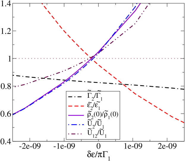
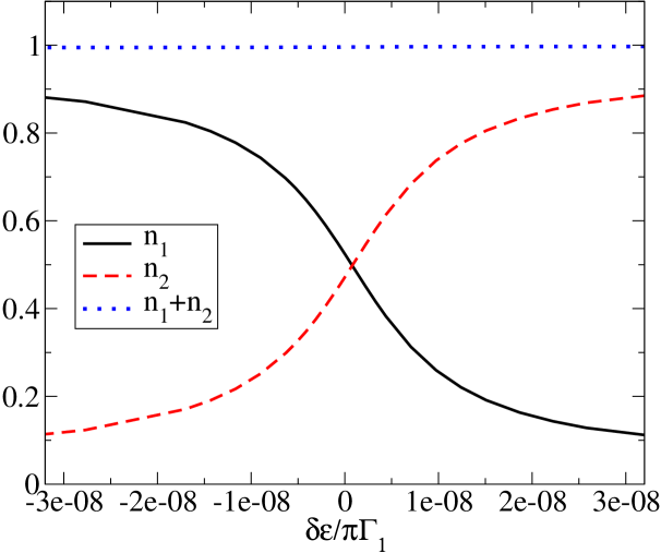
Figure 1: The ratios of renormalized parameters, $\tilde{\Gamma}_{2}/\tilde{\Gamma}_{1}$, $\tilde{\varepsilon}_{2}/\tilde{\varepsilon}_{1}$, $\tilde{\rho}^{(0)}_{2}(0)/\tilde{\rho}^{(0)}_{1}(0)$, $\tilde{U}_{2}/\tilde{U}_{1}$ and $\tilde{U}_{12}/\tilde{U}_{1}$ as a function of $\delta\varepsilon/\pi\Gamma_{1}$ for $U_{1}=U_{2}=U_{12}=0.5$, $\varepsilon_{1}=-0.093$.

Figure 2: (Color online) The occupation numbers on the individual dots, $n_{1}$, $n_{2}$, and their sum, as a function of $\delta\varepsilon/\pi\Gamma_{1}$ for the parameter set in Fig. 2.

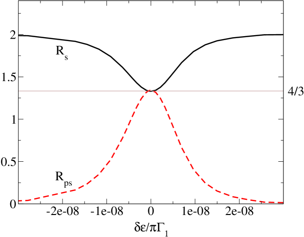
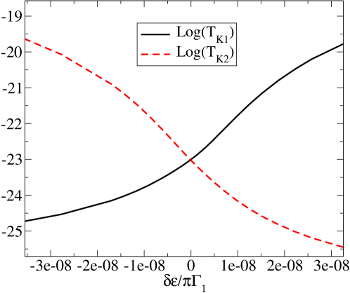
Figure 3: (Color online) The Wilson ratios for the spin and isospin, $R_{s}$ and $R_{ps}$, as a function of $\delta\varepsilon/\pi\Gamma_{1}$ for the parameter set in Fig. 2.

Figure 4: (Color online)The logarithms of the Kondo temperatures for the individual dots, $T_{\rm K,1}$ and $T_{\rm K,2}$, as a function of $\delta\varepsilon/\pi\Gamma_{1}$ for the parameter set in Fig. 2.

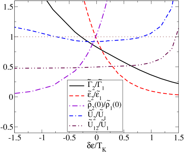
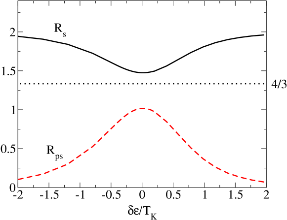
Figure 5: The ratios of renormalized parameters, $\tilde{\Gamma}_{2}/\tilde{\Gamma}_{1}$, $\tilde{\varepsilon}_{2}/\tilde{\varepsilon}_{1}$, $\tilde{\rho}^{(0)}_{2}(0)/\tilde{\rho}^{(0)}_{1}(0)$, $\tilde{U}_{2}/\tilde{U}_{1}$ and $\tilde{U}_{12}/\tilde{U}_{1}$as a function of $\delta\varepsilon/T_{\rm K}$ for the parameter set $U_{1}=U_{2}=0.05$, $U_{12}=0.03$ and $(\varepsilon_{1}+\varepsilon_{2})/2=-0.01468$.

Figure 6: (Color online) The Wilson ratios for the spin and isospin, $R_{s}$ and $R_{ps}$, plotted as a function of $\delta\varepsilon/T_{\rm K}$ for the parameter set in Fig. 6

We first of all consider the case with $U_{1}=U_{2}=U_{12}=0.5$, where we take the value $\varepsilon_{1}=-0.093$ and adjust $\varepsilon_{2}$. We cover a parameter range in which a single electron is confined to the two dots. This should be a favourable case to find a point with approximate SU(4) symmetry as we have taken the interdot repulsion $U_{12}=U_{1}=U_{2}$ and with a value comparable with $D$, similar to the situation considered by Tosi et al. The condition $U_{12}=U_{1}=U_{2}$, however, does not ensure that $\tilde{U}_{12}=\tilde{U}_{1}=\tilde{U}_{2}$ because the degree of renormalization of the spin and pseudospin fluctuations, as we shall see, can differ in general. We present results for the parameter ratios, $\tilde{\Gamma}_{2}/\tilde{\Gamma}_{1}$, $\tilde{\varepsilon}_{2}/\tilde{\varepsilon}_{1}$, $\tilde{\rho}^{(0)}_{2}/\tilde{\rho}^{(0)}_{1}$, $\tilde{U}_{2}/\tilde{U}_{1}$ and $\tilde{U}_{12}/\tilde{U}_{1}$, which are plotted in Fig.2 as a function of $\delta\varepsilon/\pi\Gamma_{1}$ ($\delta\varepsilon$ is measured relative to $\delta_{c}$, which takes the value $\delta_{c}=2.960151362\times 10^{-4}$). For complete SU(4) symmetry all these curves should intersect at the same point with a value of 1. There is a clustering of intersections about this point so to a good approximation this is the case, the exception being the ratio $\tilde{\Gamma}_{2}/\tilde{\Gamma}_{1}$. However, we have argued that for SU(4) symmetry at $\omega=0$, it is not necessary for this ratio to be equal to 1, but we do require $z_{2}/z_{1}\sim 1$. The ratio $\tilde{\Gamma}_{2}/\tilde{\Gamma}_{1}\sim 0.83$ in this regime and from $z_{2}/z_{1}=(\tilde{\Gamma}_{2}/\tilde{\Gamma}_{1})(\Gamma_{1}/\Gamma_{2})$ we deduce $z_{2}/z_{1}\approx 1.05$, which is close enough for a resticted SU(4) point. In Fig. 2 the values of occupation numbers on the dots $n_{1}$ and $n_{2}$, together with their sum $n_{\rm tot}$ are plotted over the same range, verifying that we are covering a range with $n_{\rm tot}$ very close to the value 1. Away from the restricted SU(4) fixed point we see that the ratio $\tilde{U}_{12}/\tilde{U}_{1}$ differs from the ratio $\tilde{U}_{2}/\tilde{U}_{1}$ even though we have taken, $U_{12}=U_{1}$, reflecting the fact the on-site and inter-site renormalizations differ in general.

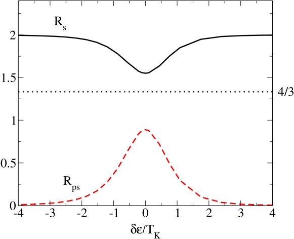
Figure 7: (Color online) The ratios of renormalized parameters, $\tilde{\Gamma}_{2}/\tilde{\Gamma}_{1}$, $\tilde{\varepsilon}_{2}/\tilde{\varepsilon}_{1}$, $\tilde{\rho}^{(0)}_{2}(0)/\tilde{\rho}^{(0)}_{1}(0)$, $\tilde{U}_{2}/\tilde{U}_{1}$ and $\tilde{U}_{12}/\tilde{U}_{1}$ for the parameter set $U_{1}=0.5$, $U_{2}=0.4$, $U_{12}=0.04$ and $(\varepsilon_{1}+\varepsilon_{2})/2=-0.0205$.

Figure 8: (Color online) The Wilson ratios for the spin and isospin, $R_{s}$ and $R_{ps}$, plotted as a function of $\delta\varepsilon/T_{\rm K}$ for the parameter set in Fig. 8.

The corresponding values of the Wilson ratios for the spin $R_{s}$ and isospin $R_{ps}$ are shown in Fig. 4 plotted against $\delta\varepsilon/\pi\Gamma_{1}$. At $\delta\varepsilon=0$ both these ratios are almost equal $4/3$ as expected at an SU(4) fixed point. Away from the SU(4) region it can be seen that the Wilson ratio for the spin $R_{s}$ takes a value 2, which corresponds to a regime in which a single electron is confined to just one of the dots. As a result in this regime there are few inter-dot fluctuations so the pseudospin Wilson ratio $R_{ps}$ drops to almost zero.

We can define Kondo temperatures for the individual dots $T_{{\rm K}i}$ via $T_{{\rm K}i}=1/4\tilde{\rho}^{(0)}_{i}(0)$ and an approximate SU(4) Kondo temperature $T^{(4)}_{{\rm K}}$ as the point where these two Kondo temperatures are equal, $T_{{\rm K}1}=T_{{\rm K}2}=T^{(4)}_{{\rm K}}$. Even though this gives a single value it does not imply a Kondo regime and universality unless all the renormalized parameters can be expressed in terms of this single energy scale. Away from the point where $T_{{\rm K}1}=T_{{\rm K}2}$ these two temperatures differ widely as can be seen in Fig. 4 , where we plot both ${\rm log}(T_{{\rm K}1})$ and ${\rm log}(T_{{\rm K}2})$ as a function of $\delta\varepsilon/\pi\Gamma_{1}$. The value of $T_{\rm K}$ at the SU(4) fixed point is very small $T_{\rm K}=1.01\times 10^{-10}$, due to the large values taken for the interactions relative to the hybridization widths.

We give some of the results for two more parameter sets with $U_{1}=U_{2}=U_{12}$ for $U_{1}/\pi\Gamma_{1}=12$ and $U_{1}/\pi\Gamma_{1}=5$ in Table I. These interaction terms are much reduced from the set we have just considered in detail, but they are still in the Kondo regime with the inter-dot charge fluctuations suppressed. In both cases there is a point corresponding to an restricted SU(4) fixed point but, with the reduced values of the interaction parameters, the Kondo temperatures are significantly bigger.

In the next parameter set given in Table I, all the interactions terms are significantly larger than the bandwidth, $U_{1}/D=U_{2}/D=5$, $U_{12}/D=3$ ($D=1$), but the inter-site term is reduced relative to the on-site interactions, reflecting a more realistic double dot situation. We see again that there is a good restricted SU(4) fixed point. So the reduction in the value of $U_{12}$ relative to $U_{1}$ and $U_{2}$ does not at first sight have made any significant difference. However, the value of the Kondo temperature is very much bigger than for the set $U_{1}=U_{2}=U_{12}=0.5$ with smaller values of the interactions.

In the next set in Table I we have the results for a case where the interaction parameters are reduced to be much less than the bandwidth, $U_{1}/D=U_{2}/D=0.05$, $U_{12}/D=0.03$ ($(\varepsilon_{1}+\varepsilon_{2})/2=-0.01468$) but still in the strong correlation regime. The results for the ratios of the renormalized parameters and the Wilson ratios are shown in Figs. 6 and 6 plotted as a function of $\delta\varepsilon/T_{\rm K}$, with $T_{\rm K}$ as defined earlier as the value where $T_{{\rm K}1}=T_{{\rm K}2}=T_{\rm K}$. We see that these results are in marked contrast to the similar set with $U_{1}=U_{2}=U_{12}=0.05$, which differs from this set only in the value of $U_{12}$. A comparison of the results in Fig. 6 with those Fig. 2 shows that, though there is an approximate point where most of the ratios take a value of order 1, the ratio $\tilde{U}_{12}/\tilde{U}_{1}$ falls well below this point. As a consequence we see in Fig. 6 that though there is a peak in $R_{ps}$ and a dip in $R_{s}$ neither of these attain the required value of $4/3$ for a universal SU(4) Kondo fixed point. As the peak in $R_{ps}$ is greater than 1, we can classify the fixed point as an approximate SU(4) Kondo fixed point.

We see similar results in Figs. 8 and 8 corresponding to the parameter set, $U_{1}=0.5$, $U_{2}=0.4$, $U_{12}=0.04$ ($(\varepsilon_{1}+\varepsilon_{2})/2=0.007896$). In this case the ratio $z_{2}/z_{1}=1.12$ giving a significant deviation from 1. Also as $R_{ps}<1$, by our criteria the fixed point in this case does not qualify as an approximate SU(4) fixed point. The results are very similar in the other case considered; $U_{1}=1.0$, $U_{2}=0.8$, $U_{12}=0.1$, but with the larger value of $U_{12}$ we find an approximate SU(4) point as $R_{ps}>1$.

We conclude from these examples, with $U_{1}=U_{2}=U_{12}$ but with asymmetry of the coupling so that $\Gamma_{1}\neq\Gamma_{2}$, that it is possible in the Kondo regime with $n_{1}+n_{2}\sim 1$, to achieve to a good approximation a restricted energy SU(4) fixed point by adjusting the difference in energy levels, $\varepsilon_{1}-\varepsilon_{2}$, in line with the conclusions of Tosi et al. The shifts $\delta_{c}$ required to obtain this point in all our examples is of the same order of magnitude $\sim 10^{-4}$. Tosi et al. were able to relate this shift quantitatively to the formula for the Haldane scaling. This we were not able to do here, but for $U\to\infty$ and $U_{12}\to\infty$ there is only one relevant cut-off $C=|\varepsilon|$. With finite and different values of both $U$ and $U_{12}$ in our examples, the charge scaling regimes will have different lower cut-offs so no simple universal formula is likely to apply.

We also found a restricted SU(4) fixed point for $U_{12}<U_{1}$, $U_{12}<U_{2}$ but only for $U_{12}$ greater than the conduction band width $D$, ie. $U_{12}>1$. However, for $U_{12}/\pi\Gamma_{1}\gg 1$ but $U_{12}<1$, we find only a non-universal approximate SU(4) fixed point. This indicates at the low energy regime the inter-dot and on-site interactions act differently.

IV.1 NRG Spectral Densities

We now examine some of the results at a restricted SU(4) fixed point with $n_{\rm tot}\sim 1$ on higher energy scales. We look first of all at a case with identical dots and hybridizations, $\pi\Gamma_{1}=\pi\Gamma_{2}=0.01$, and $U_{1}=U_{2}=U_{12}=0.12$, which has SU(4) symmetry on all energy scales. We expect the free quasiparticle expression $z\rho^{(0)}(\omega)$ to give a good approximation to the full spectral density $\rho(\omega)$ in the low frequency regime near the Fermi level. To test this we plot the ratios $\rho(\omega)/\rho(0)$ and $\tilde{\rho}^{(0)}(\omega)/\tilde{\rho}^{(0)}(0)$ as a function of $\omega$ in Fig. 9. We see that this is indeed the case and the quasiparticle result accurately reproduces the sharp rise in the spectral density in the low energy regime.

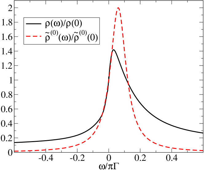
Figure 9: (Color online). Plots of $\rho(\omega)/\rho(0)$ and $\tilde{\rho}^{(0)}(\omega)/\tilde{\rho}^{(0)}(0)$ for an SU(4) model with $n_{\rm tot}=1$ for $U_{12}=U_{1}=U_{2}=0.05$, $\pi\Gamma_{1}=\pi\Gamma_{2}=0.01$.

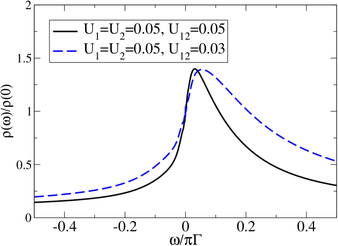
Figure 10: (Color online). Plots of $\rho(\omega)/\rho(0)$ for the parameter set as in 9, and for almost the same set except with a reduced value of $U_{12}=0.03$.

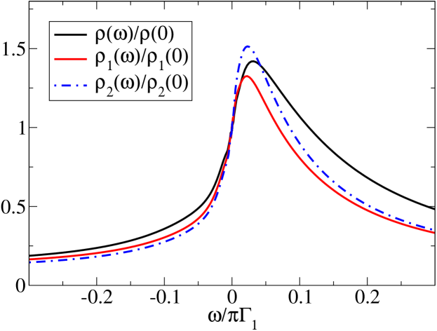
Figure 11: (Color online) A plot of $\rho(\omega)/\rho(0)$ for the parameter set given in Fig. 9 and $\rho_{1}(\omega)/\rho_{1}(0)$ and $\rho_{2}(\omega)/\rho_{2}(0)$ for a model with the same interaction parameters ($U_{12}=U_{1}=U_{2}=0.05$) but with $\pi\Gamma_{1}=0.01$ and $\pi\Gamma_{2}=0.007896$.

In Fig. 10 we give two plots of $\rho(\omega)/\rho(0)$ for identical dots $n_{1}=n_{2}=1/2$, one for the set $U_{1}=U_{2}=U_{12}=0.05$ and the other for $U_{1}=U_{2}=0.05$, $U_{12}=0.03$. The first corresponds to an SU(4) fixed point with a Wilson ratio, $R_{s}=R_{ps}=1.329$, the second set with $R_{s}=1.48$ and $R_{ps}=1.005$, so corresponds only to an approximate SU(4) fixed point. Though the spectral densities have the same value at the Fermi level, $\rho(0)\sim 1/2\pi\Gamma$, they deviate away from this point. Such a deviation would be expected even if both sets corresponded to an SU(4) fixed point because they would have different values of $T_{\rm K}^{(4)}$, but the comparison does reveal that the reduction in $U_{12}$ significantly affects the spectrum on all energy scales.

In Fig. 11 we compare $\rho(\omega)/\rho(0)$ for two sets both with $U_{1}=U_{2}=U_{12}=0.05$, but set 1 with $\pi\Gamma_{1}=\pi\Gamma_{2}=0.01$ and set 2 with $\pi\Gamma_{1}=0.01$, $\pi\Gamma_{2}=0.007896$. In each case the levels are adjusted to give an SU(4) point $n_{\rm tot}=1$. In the second set the difference between the energy levels has to be adjusted so that the effective levels coincide. As consequence the spectral density on two dots, $\rho_{1}(\omega)$ and $\rho_{2}(\omega)$ differ. Nevertheless all the spectral densities remain very close in the low energy regime near the Fermi level, indicating that the SU(4) symmetry can largely be restored in this regime by adjusting the difference in the levels on the dots, but not on the higher energy scales.

V Dependence on on-site and inter-site interactions

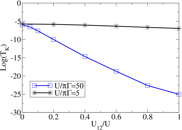
Figure 12: (Color online) A plot of $\tilde{U}/2\pi\tilde{\Gamma}$ (higher curves) and $\tilde{U}_{12}/2\pi\tilde{\Gamma}$ (lower curves) against the ratio $U_{12}/U$ for the model with $n_{tot}=1$ for $U/\pi\Gamma=5,50$ and $\pi\Gamma=0.01$.

Figure 13: (Color online) A plot of ${\rm log}(T_{\rm K})$ versus $U_{12}/U$ for the same parameter sets as in Fig. 13.

We now investigate more systematically how close we can approach an SU(4) fixed point given the interaction parameters $U_{12}$ and $U_{1}=U_{2}=U$, without the complication of different couplings so we take $\Gamma_{1}=\Gamma_{2}$. For a given value of $U$ and $\pi\Gamma=0.01$, we calculate the values of $\tilde{U}_{12}/2\pi\tilde{\Gamma}$ and $\tilde{U}/2\pi\tilde{\Gamma}$ as a function of $U_{12}/U$, with $\varepsilon_{1}=\varepsilon_{2}=\varepsilon$ determined by the constraint $n_{1}=n_{2}=1/2$. For an SU(4) fixed point we require $\tilde{U}_{12}/2\pi\tilde{\Gamma}=\tilde{U}/2\pi\tilde{\Gamma}$ and for a universal strong coupling Kondo fixed point they should both take the value $1/3$. In Fig. 13 we show two such plots, one for $U/\pi\Gamma=5$ and a second for $U/\pi\Gamma=50$. For $U/\pi\Gamma=5$ we see a steady increase of $\tilde{U}_{12}/2\pi\tilde{\Gamma}$ with $U_{12}/U$ and a steady decrease of $\tilde{U}/2\pi\tilde{\Gamma}$, but not until $U_{12}=U$ do they become equal. For the much larger value of $U$, $U/\pi\Gamma=50$, there is an initial accelerated increase in $\tilde{U}_{12}/2\pi\tilde{\Gamma}$ with $U_{12}/U$, mirrored by a corresponding decrease in $\tilde{U}/2\pi\tilde{\Gamma}$, with the two curves moving much closer. However, even with this value of $U$, comparable with the band with $D=1$ ($U=D/2$), we do not get full SU(4) symmetry until $U_{12}=U$. In both cases the value $U$ is large enough when $U_{12}=U$ to give the universal strong correlation Kondo value $1/3$.

There is an interesting difference in the degree of renormalization in these two cases evident in the plot of ${\rm log}(T_{\rm K})$ shown in Fig. 13. The Kondo temperature is a measure of the degree of renormalization as the quasiparticle weight factor $z$ is given by $z=2T_{\rm K}/\pi\Gamma$. For $U_{12}=0$, there is only a modest degree of renormalization both for $U/\pi\Gamma=5$, $z=0.641$ and $U/\pi\Gamma=50$, $Z=0.495$ as $U$ suppresses only the double occupation on each dot, so charge fluctuations between $n=0$ and $n=1$ are largely unaffected. Once $U_{12}$ is switched on these remaining charge fluctuations are also suppressed and the SU(4) Kondo limit, $\tilde{U}_{12}\tilde{\rho}^{(0)}(0)\to 1/3$, is approached in both cases. However, at this point for $U/\pi\Gamma=5$, we find $z=0.191$, being reduced by a factor of the order of 3, whereas for $U/\pi\Gamma=50$, $z=2.71\times 10^{-9}$, reduced by a factor of the order $2\times 10^{8}$. The dramatic difference between the two cases can be seen in Fig. 13 where the results for ${\rm log}(T_{\rm K})$ are plotted as a function of $U_{12}/U$. This difference in behavior in the two cases can be related to the form of their spectral densities which are shown in Figs. 14 and 15. In Fig. 14 the spectral densities are shown for the parameter sets, $U/\pi\Gamma=5$, for $U_{12}/U=0,0.4$ and $0.8$. There is just one peak above the Fermi level, which does shift closer to the Fermi level and narrow as $U_{12}$ is increased. The value of bare level parameter $\varepsilon$ to give $n=1/2$ for these three cases are $\varepsilon/\pi\Gamma=-0.144,-1.08,-1.82$, all fall below the Fermi level. From the Friedel sum rule, we know that $n=1/2$ implies $\tilde{\varepsilon}=\tilde{\Gamma}$, so the quasiparticle peak has to lie above the Fermi level, so the peak in the spectrum is essentially that due to the renormalized quasiparticles. It can also be interpreted as the shifted peak $\varepsilon^{*}$ due to Haldane scaling. Haldane scaling, however, does not take into account any wavefunction renormalization, but the two shifts can be related by interpreting $\varepsilon^{*}$ as $\varepsilon+\Sigma(0)$, so that $\varepsilon^{*}=\tilde{\varepsilon}/z$.

The spectral densities for the larger $U$ case, $U/\pi\Gamma=50$, for $U_{12}/U=0,0.2$ and $0.4$ are shown in Fig. 15. The corresponding values of $\varepsilon$ are $\varepsilon/\pi\Gamma=-0.408,-4.14,-6.80$. There is now a very significant change when the inter-site interaction $U_{12}$ is switched on. There is a very dramatic narrowing of the quasiparticle peak above the Fermi level and at the same time two other peaks appear. The one below the Fermi level can be identified as associated with the ‘atomic’ level at $\omega=\varepsilon$, and the higher peak above the Fermi level as the atomic level at $\omega=\varepsilon+U_{12}$. The picture emerging for larger $U_{12}$ begins to look similar to that for a single Anderson model near particle-hole symmetry with a three peak structure and an exponentially renormalized Kondo peak.

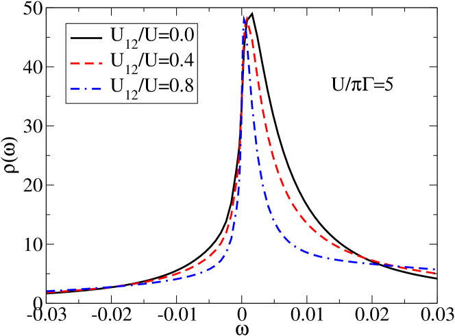
Figure 14: (Color online) A plot of $\rho(\omega)$ against $\omega$ for ratios $U_{12}/U=0.0,0.2,0.4$ for $U=0.05$ and $\pi\Gamma=0.01$.

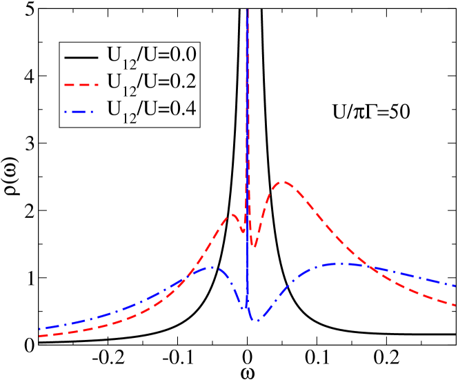
Figure 15: (Color online) A plot of $\rho(\omega)$ against $\omega$ for ratios $U_{12}/U=0.0,0.2,0.4$ for $U=0.5$ and $\pi\Gamma=0.01$.

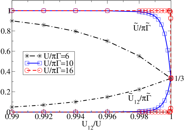
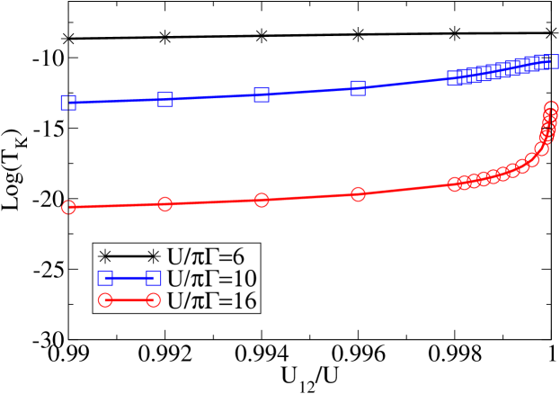
Figure 16: (Color online) A plot of $\tilde{U}/\pi\tilde{\Gamma}$ (higher curves) and $\tilde{U}_{12}/\pi\tilde{\Gamma}$ (lower curves) against the ratio $U_{12}/U$ for the particle-hole symmetric model with $n_{tot}=2$ for $U/\pi\Gamma=6,10,16$ and $\pi\Gamma=0.01$.

Figure 17: (Color online) A plot of ${\rm log}(T_{\rm K})$ versus $U_{12}/U$ for the same parameter sets as in Fig. 17.

It might be surprising that the condition $U_{12}/\pi\Gamma_{1}>5$ is not sufficient to lead to an SU(4) Kondo fixed point for $n_{\rm tot}=1$. A similar situation also occurs in the Kondo regime for the double dot with $n_{\rm tot}=2$. For two identical dots with particle-hole symmetry, $U_{12}=U_{1}=U_{2}=U$ and $U/\pi\Gamma\gg 1$, the model maps into an SU(4) Kondo model, with the operators corresponding to a 6-dimensional representation, rather than the 4-dimensional representation for $n_{\rm tot}=1$. In earlier calculationsNishikawa et al. (2012a) for $U_{12}<U$ with $U/\pi\Gamma=5$, we found only an SU(2) fixed point as $\tilde{U}_{12}\sim 0$, until $U_{12}$ almost reached the value $U$, and then a very rapid cross-over to an SU(4) fixed point as $U_{12}\to U$. It might be argued that increasing $U/\pi\Gamma$ will increase the range of $U_{12}/U$ favouring the SU(4) fixed point. However, we find the opposite is the case. In Fig. 17 (i) we plot both $\tilde{U}/\pi\tilde{\Gamma}$ and $\tilde{U}_{12}/\pi\tilde{\Gamma}$ as a function of $U_{12}/U$ for two identical particle-hole symmetric dots with $U/\pi\Gamma=6,10,16$ and $\pi\Gamma=0.01$. We see that for $U/\pi\Gamma=10$, we have a clear SU(2) fixed point with $\tilde{U}/\pi\tilde{\Gamma}=1$ and $\tilde{U}_{12}/\pi\tilde{\Gamma}\sim 0$ over 99.8% of the range of $U_{12}/U$ and an even greater range for $U/\pi\Gamma=16$. This reinforces the assertion that inter-dot repulsion plays a rather different role on the lowest energy scales compared with the on-site term.

In Fig. 17 we plot the corresponding values of ${\rm log}(T_{\rm K})$ as a function of $U_{12}/U$ for the parameter sets shown in Fig. 17. There is very little change until $U_{12}/U>0.998$ at which point there is an increase in $T_{\rm K}$ on the approach to the SU(4) point $U_{12}=U$, which is particularly marked for the larger value of $U$. This is precisely opposite behavior in the approach to the SU(4) fixed point to that for $n_{\rm tot}=1$. In Fig. 18 the spectral density $\rho(\omega)$ is shown for a particle-hole symmetric case for the sets, $U_{12}=U_{1}=U_{2}=0.05$ and $U_{12}=0.03$, $U_{1}=U_{2}=0.05$. There is a broad Kondo peak at the Fermi level for the first case corresponding to an SU(4) fixed point, and an exponentially narrowed one corresponding to an SU(2) fixed point for the second with a smaller value of $U_{12}$.

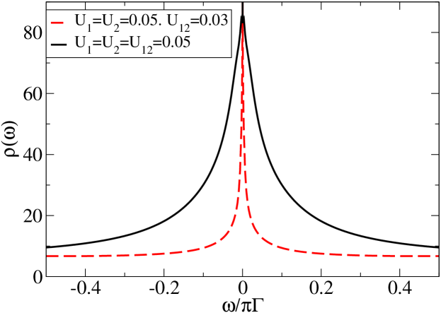
Figure 18: (Color online) A plot of $\rho(\omega)$ as a function of $\omega/\pi\Gamma$ for a particle-hole symmetric SU(4) model with $U_{12}=U_{1}=U_{2}=0.05$ compared with $\rho(\omega)$ for the set $U_{12}=0.03$, $U_{1}=U_{2}=0.05$ ($\pi\Gamma_{1}=\pi\Gamma_{2}=0.01$).

VI Temperature dependence of the differential conductance

As mentioned in the introduction the measurement of the differential conductance through a quantum dot, or arrangement of quantum dots, has become an important way to probe locally strongly correlated states, which can be performed under equilibrium or non-equilibrium conditions. A general formula for calculating the conductance for a single dot $i$ subject to a bias voltage $V_{i}$ was derived by Meir and Wingreen Meir and Wingreen (1992), and takes the form,

$$I_{i}=\frac{4e\bar{g}_{i}}{\pi\hbar}\!\int\limits_{-\infty}^{\infty}\!\!{\rm d}\omega\;[f_{s}(\omega)-f_{d}(\omega)][-{\rm Im}G^{r}_{i}(\omega,T,V_{ds,i})],$$ (19)

where $\bar{g}_{i}=\Gamma_{d,i}\Gamma_{s,i}/(\Gamma_{d,i}+\Gamma_{s,i})$, $G_{i}^{r}(\omega,T,V_{ds,i})$ is the steady state retarded Green’s function on the dot site, and $f_{s}(\omega)$, $f_{d}(\omega)$ are Fermi distribution functions for the electrons in the source and drain reservoirs, respectively, $f_{\alpha}(\omega)=f_{\rm F}(\omega-\mu_{\alpha})$ and $\mu_{s,i}=\alpha_{s,i}eV_{i}$, $\mu_{d,i}=-\alpha_{d,i}eV_{i}$, so that for a difference in chemical potential across dot $i$ of $eV_{i}$ due to the bias voltage, $V_{i}$, $\alpha_{s,i}+\alpha_{d,i}=1$. To evaluate this expression we need the retarded Green’s function as a function of the bias voltage $V_{ds,i}$. It is proving to be a difficult and challenging problem to extend the many-body techniques, such as the NRG, which can be reliably used to tackle local strong correlation problems under equilibrium conditions, to non-equilibrium situations. However, the equilibrium Green’s function is sufficient to calculate the zero bias conductance, and if the coupling of the drain to the source can be made very small, $\Gamma_{i,d}/\Gamma_{i,s}\ll 1$, then it can be argued that the very weak current is probing the equilibrium state of the dot. Under these conditions useful information can be obtained from equilibrium calculations.

We first of all look at the leading low temperature corrections to the zero bias conductance,

$$G_{i}(T)=\frac{4e\bar{g}_{i}}{\hbar}\!\int\limits_{-\infty}^{\infty}\!\!{\rm d}\omega\;\beta\mathrm{e}^{\beta\omega}f_{\rm F}(\omega)^{2}\rho_{i}(\omega,T),$$ (20)

where $\beta=1/T$. To evaluate this expression in the low temperature regime, we use the spectral density on a given dot in terms of the renormalized parameters which is given by

$$\rho(\omega,T)=z\tilde{\rho}(\omega,T)=\quad\quad\quad\quad\quad$$

$$\frac{1}{\pi\Gamma}\frac{\tilde{\Gamma}(\tilde{\Gamma}-\tilde{\Sigma}^{I}(\omega,T))}{(\omega-\tilde{\varepsilon}-\tilde{\Sigma}^{R}(\omega,T))^{2}+(\tilde{\Gamma}-\tilde{\Sigma}^{I}(\omega,T))^{2}},$$ (21)

where $\tilde{\Sigma}^{R}(\omega,T)$ and $\tilde{\Sigma}^{I}(\omega,T)$ are the real and imaginary parts of the renormalized self-energy. For a Fermi liquid fixed point both $\tilde{\Sigma}^{R}(\omega,T)$ and $\tilde{\Sigma}^{I}(\omega,T)$ and their first derivatives with respect to $\omega$ are zero at $\omega=0$. The leading order temperature corrections in the Fermi liquid regime are of order $T^{2}$ so to evaluate the expression for $G(T)$ to this order we need the renormalized self-energy to order, $\omega^{2}$ and $T^{2}$. We calculate these up to second order in powers of the renormalized quasiparticle interaction $\tilde{U}$ using the renormalized perturbation theory RPTHewson (1993), and details of the calculation are given in the Appendix.

We give the result first of all for the particle-hole symmetric case $n_{tot}=2$, which is exact to this order as it depends only on the imaginary part of the renormalized self-energy,

$$G(T)=G(0)\left[1-(1+\phi)\frac{\pi^{4}}{48}\left(\frac{T}{T_{\rm K}}\right)^{2}+{\rm O}(T^{4})\right],$$ (22)

where $\phi=2(\tilde{U}^{2}+2\tilde{U}_{12}^{2})/(\pi\tilde{\Gamma})^{2}$ is the term arising from the quasiparticle interactions. In the SU(2) case, $\tilde{U}/\pi\tilde{\Gamma}=1$ and $\tilde{U}_{12}=0$, so $\phi^{(2)}=2$. For SU(4) with particle-hole symmetry, $\tilde{U}_{12}=\tilde{U}$ and $\tilde{U}/\pi\tilde{\Gamma}=1/3$, so $\phi^{(4)}=2/3$. We note that the correction term due to the quasiparticle interactions is smaller in the SU(4) case. This is in line with results for $N$-fold degenerate Anderson and Kondo models, where the effects of the quasiparticle interactions tend to zero in a suitably scaled large $N$ limit. We also note that leading term is negative so that the very low temperature conductance decreases with temperature.

In contrast the result for the SU(4) model with $n_{\rm tot}=1$ has an initial increase with temperature and takes the form,

$$G(T)=G(0)\left[1+(1-\psi)\frac{\pi^{4}}{24}\left(\frac{T}{T_{\rm K}}\right)^{2}+{\rm O}(T^{4})\right],$$ (23)

where $\psi$ is the correction due to the quasiparticle interactions, which arises in this case solely from the real part of the self-energy Hur et al. (2007). We evaluate this term to order $\tilde{U}^{2}$ in the RPT, corresponding to the diagrams shown in Fig. 19. The total contribution to $\psi$ from the tadpole diagram Fig. 19 (i) is $-(\pi/2-1)(\tilde{U}^{2}+2\tilde{U}_{12}^{2})/(4\pi\tilde{\Gamma})^{2}$ or $-0.1903$, and from the second order diagram in Fig. 19 (ii) $-0.2652(\tilde{U}^{2}+2\tilde{U}_{12}^{2})/(4\pi\tilde{\Gamma})^{2}$ or $-0.0884$. The net result for $\psi$ is $\psi=-0.279$. There can be higher order corrections as the second order result for the real part of the renormalized self-energy is not exact to second order. However, this result can be expected to be a reasonable order of magnitude estimate of the corrections arising from the quasiparticle interactions. We note that in this case there is an initial increase of $G(T)$ with $T$.

The difference in the behavior of $G(T)$ for the SU(4) cases with $n_{\rm tot}=2$ and $n_{\rm tot}=1$ can be related to the differences in their spectral densities $\rho(\omega)$ for small $\omega$. For $n_{\rm tot}=2$ the spectral density has a narrow Kondo peak centred at the Fermi level so the spectral density falls off from $\omega=0$ with a negative curvature. When $n_{\rm tot}=1$, on the other hand, the Kondo peak is at $\omega\sim T_{\rm K}$ above the Fermi level, so initially rises strongly from $\omega=0$ with positive curvature, leading to an increase of conductance with temperature. There is a corresponding contrast in low $T$ behavior in other physical properties of SU(N) models. For example, the impurity susceptibility $\chi(T)$ of an SU(N) Kondo modelRajan (1983) shows an initial rise and a maximum with increase of $T$ for $N>3$ (though the peak is a relatively shallow one for $N=4$) and an initial decrease for $N=2$. This difference can be understood in terms of the quasiparticle density of states,

$$\tilde{\rho}(\omega)=\frac{1}{\pi}\frac{\tilde{\Gamma}}{(\omega-\tilde{\varepsilon})^{2}+\tilde{\Gamma}^{2}},$$ (24)

and the Friedel sum rule,

$$n=1-\frac{2}{\pi}{\rm tan}^{-1}\left(\frac{\tilde{\varepsilon}}{\tilde{\Gamma}}\right).$$ (25)

The result for the sum rule can be obtained by integrating the quasiparticle density of states up to the Fermi level. Hence for $n=1$ ($n_{tot}=2$, half filling), the quasiparticle density of states has to be centred at the Fermi level, whereas for $n=2/N$, $N>2$ ($1/N$th filling), the quasiparticle peak has to lie above the Fermi levelHewson (1997). For $n=1/2$ ($n_{\rm tot}=1$) and $N=4$, the peak is a $\omega=\tilde{\varepsilon}=\tilde{\Gamma}=2T_{\rm K}/\pi$, so we have an upward curvature in $\tilde{\rho}(\omega)$, and a consequent initial increase of the conductance with temperature.

VII Conclusions

To observe a low energy SU(4) Kondo fixed point behavior in a capacitively coupled quantum dot we have to isolate a single electron on the double dot system, by suppressing charge fluctuations on the individual dots and also between the dots, such that the occupation number on each dot $n_{i}=1/2$. From the Friedel sum rule this implies that quasiparticle density of states, specified by a peak at $\omega=\tilde{\varepsilon}$ with a width $\tilde{\Gamma}$, must be a quarter filled with $\tilde{\varepsilon}=\tilde{\Gamma}$. The general condition to suppress charge fluctuations on a single dot (for $U_{12}=0$) is that $U\rho(0)\gtrsim 2$, so as $\rho(0)=1/2\pi\Gamma$ quarter filling, this implies a value of $U$ such that $U/\pi\Gamma\gtrsim 4$. On switching on an inter-dot interaction we also need a value of $U_{12}$ such that $U_{12}/\pi\Gamma\gtrsim 4$ to suppress the inter-dot charge fluctuations. What is somewhat unexpected in our results is that these two conditions are not sufficient to generate an SU(4) symmetric fixed point with universal spin and pseudospin Wilson ratios, $R_{s}=R_{ps}=4/3$. Our calculations indicate that these conditions are satisfied only asymptotically as $T_{\rm K}\to 0$. However, the low energy behavior of a double dot system with $U>U_{12}>4\pi\Gamma$, will not depend significantly on satisfying the strict criteria for SU(4) symmetry. It depends on the form of the low energy quasiparticle spectrum, which under these conditions corresponds to a narrow resonance just above the Fermi level. The larger the value of $U_{12}$ ($<U$) the greater degree of renormalization and the narrower the quasiparticle resonance. Hence the low energy behavior depends on two factors, the position of the quasiparticle resonance, which is determined by the Friedel sum rule, and the degree of renormalization, determined by the degree to which that charge fluctuations on the individual dots and between the dots can be suppressed.

The presence of the narrow quasiparticle resonance just above the Fermi level should be reflected in the experimentally measured temperature dependence of the linear conductance through a given dot, $G(T)$. This should result in an initial increase of $G(T)$ and a maximum in contrast to the monotonic decrease which occurs when the quasiparticle peak is located at the Fermi level. This increase is not seen in the experimentsKeller et al. (2014) reporting universal SU(4) temperature dependence in a capacitatively coupled double quantum dot, though an initial rise is evident in the NRG calculations, with which they are compared. It can be argued that an initial rise with temperature leading to a maximum is a clearer universal characteristic low temperature feature of a SU(4) Kondo model with $n_{tot}=1$, as it shows up in several low temperature properties, such as in the universal temperature dependent susceptibilityRajan (1983), $\chi(T)$ and the universal magnetic field dependent susceptibility $\chi(H)$Hewson and Rasul (1983) at $T=0$. It does not depend on having a precise SU(4) fixed point, but only on having a narrow resonance above the Fermi level, which is a consequence of the Friedel sum rule and the constraint $n_{\rm tot}=1$ ($n_{1}=n_{2}=1/2$). In the SU(4) $n_{\rm tot}=1$ Kondo limit there is no particle-hole symmetry for finite $T_{\rm K}$ as the peak in the quasiparticle spectrum is at $\omega=2T_{\rm K}/\pi$.

The position of the quasiparticle peak above the Fermi level also results in a much slower fall off of $G(T)$ with temperature at higher temperatures, than in the SU(2) case with a Kondo resonance at the Fermi level. In our earlier workNishikawa et al. (2013) we showed that the features seen in the measurementsKeller et al. (2014) of $G(T)$ in the higher temperature range, as a function of the dot energy level $\varepsilon$, can be interpreted in terms of the temperature dependence of the renormalized parameters for the quasiparticles. The temperature of these parameters can be estimated from the NRG calculations.

The other issue we have considered here is the effect of the dots having different couplings to their baths, $\Gamma_{1}\neq\Gamma_{2}$, which breaks the symmetry between the dots. Tosi et al. showed that for $U=U_{12}=\infty$, the symmetry on a low energy scale could be effectively restored by adjustment of the energy levels on the individual dots via the applied gate voltages. Our calculations for finite $U$ and $U_{12}$, are largely in agreement with their conclusions but restricted to the lowest energy scale. For $U_{12}<U$, our conclusions are in line with the case of identical dots, that there is only an approximate SU(4) fixed point unless both $U$ and $U_{12}$ are greater than $D$.

VIII Acknowledgements

Numerical computation in this work was partially carried out at the Yukawa Institute Computer Facility. This work has been supported in part by the EPSRC Mathematics Platform grant EP/1019111/1. One of us (OC) acknowledges the support of an EPSRC DTA grant EP/K502856/1. YN also acknowledges the support by JSPS KAKENHI Grant Number 15K05181.

IX Appendix

We use the renormalized perturbation theory (RPT) Hewson (1993) to estimate the low temperature corrections arising from the interaction between the quasiparticles. The spectral density $\rho(\omega,T)$ is given by

$$\rho(\omega,T)=\frac{z}{\pi}\frac{\tilde{\Gamma}-\tilde{\Sigma}^{I}(\omega,T)}{(\omega-\tilde{\varepsilon}-\tilde{\Sigma}^{R}(\omega,T))^{2}+(\tilde{\Gamma}-\tilde{\Sigma}^{I}(\omega,T))^{2}},$$ (26)

where $\tilde{\Sigma}^{R}(\omega,T)$ and $\tilde{\Sigma}^{I}(\omega,T)$ are the real and imaginary parts of the renormalized self-energy. To calculate the leading low frequency and low temperature corrections to $\rho(\omega,T)$ we can use the fact that at a Fermi liquid fixed point that $\tilde{\Sigma}_{I}(\omega,T)$ and $\tilde{\Sigma}_{R}(\omega,T)$ are both of order $\omega^{2}$ or $T^{2}$ as $\omega\to 0$ and $T\to 0$, we need only include these terms to lowest order,

$$\frac{\rho(\omega,T)}{\rho(0,0)}=1+\pi^{2}\omega^{2}(\tilde{\rho}^{(0)}(0,0))^{2}\left(\frac{3\tilde{\varepsilon}^{2}}{\tilde{\Gamma}^{2}}-1\right)$$

$$+\left(1-\frac{\tilde{\varepsilon}^{2}}{\tilde{\Gamma}^{2}}\right)\pi\tilde{\rho}^{(0)}(0,0)\tilde{\Sigma}_{I}(\omega,T)$$

$$-\frac{2\pi\tilde{\varepsilon}\tilde{\rho}^{(0)}(0,0)\tilde{\Sigma}_{R}(\omega,T)}{\tilde{\Gamma}}+\frac{2\pi\tilde{\varepsilon}\omega\tilde{\rho}^{(0)}(0,0)}{\tilde{\Gamma}}.$$ (27)

In the particle-hole symmetric case, $\tilde{\varepsilon}=0$ this simplifies to

$$\frac{\rho(\omega,T)}{\rho(0,0)}=1-\pi^{2}\omega^{2}(\tilde{\rho}^{(0)}(0,0))^{2}+\pi\tilde{\rho}^{(0)}(0,0)\tilde{\Sigma}_{I}(\omega,T),$$ (28)

so to evaluate this we need only the calculation of $\tilde{\Sigma}_{I}(\omega,T)$. To order $\omega^{2}$ and $T^{2}$ it is given exactly within the second order in the renormalized perturbation theory Hewson (1993); Nishikawa et al. (2012b),

$$\tilde{\Sigma}_{I}(\omega,T)=-\frac{\pi}{2}(\tilde{\rho}^{(0)}(0))^{3}(\tilde{U}^{2}+2\tilde{U}_{12}^{2})(\omega^{2}+\pi^{2}T^{2}).$$ (29)

In the SU(4) case with $\tilde{\varepsilon}=\tilde{\Gamma}$, $n=1/2$ on each dot,

$$\frac{\rho(\omega,T)}{\rho(0,0)}=1+{2}\pi^{2}\omega^{2}(\tilde{\rho}^{(0)}(0,0))^{2}\quad\quad$$

$$-2\pi\tilde{\rho}^{(0)}(0,0)\tilde{\Sigma}_{R}(\omega,T)+2\pi\omega\tilde{\rho}^{(0)}(0,0).$$ (30)

In this case the imaginary part of the renormalized self-energy makes no contribution to lowest order, but we need to evaluate the real part. We can estimate this to second order in the RPT expansion. There is a contribution to first order in $\tilde{U}$ and $\tilde{U}_{12}$ from the simple tadpole diagram (see 19 (i)) given by

$$\tilde{\Sigma}^{(1)}_{R}(T) = \frac{\tilde{U}+2\tilde{U}_{12}}{2}(n^{(0)}(T)-n^{(0)}(0))$$ (31)

$$= -\frac{(\tilde{U}+2\tilde{U}_{12})\tilde{\varepsilon}(\tilde{\rho}^{(0)}(0,0))^{2}\pi^{3}T^{2}}{3\tilde{\Gamma}}.$$

There is also a second order tadpole diagram, which is essentially a first order mean field correction to the first order tadpole diagram. The mean field equation takes the form,

$$\delta n(T)=1-\frac{2}{\pi}{\rm tan}^{-1}\left(\frac{\tilde{\varepsilon}+\tilde{U}\delta n(T)/2}{\tilde{\Gamma}}\right),$$ (32)

where $\delta n(T)=n(T)-n(0)$. Iterating this equation to first order in $\tilde{U}$, we obtain the second order correction from the second order tadpole diagram as

$$\frac{(\tilde{U}+2\tilde{U}_{12})^{2}\tilde{\varepsilon}(\tilde{\rho}^{(0)}(0,0))^{3}\pi^{3}T^{2}}{3\tilde{\Gamma}}.$$ (33)

In the renormalized perturbation theory there are counter terms to take into account. The only counter term we have to take explicitly into account in this second order calculation is a $\lambda_{3}$ counter term which is required to cancel off any zero frequency 4-vertex terms, as these have been fully included already in the definitions of $\tilde{U}$ and $\tilde{U}_{12}$. Away from particle-hole symmetry there is a second order contribution to $\lambda_{3}$ given by

$$\lambda_{3}=\tilde{U}^{2}\left(\tilde{\rho}^{(0)}(0)-\frac{1}{\pi\tilde{\varepsilon}}{\rm tan}^{-1}\left(\frac{\tilde{\varepsilon}}{\tilde{\Gamma}}\right)\right),$$ (34)

arising from the diagrams shown in Fig 20. The counter term $\lambda_{3}$ is best handled by carrying out the expansion in powers of $\tilde{U}-\lambda_{3}$. Hence it will give a second order contribution to the simple tadpole diagram, given by

$$-\lambda_{3}\delta n^{(0)}(T)=\frac{(\tilde{U}^{2}+2\tilde{U}_{12}^{2})\tilde{\varepsilon}(\tilde{\rho}^{(0)}(0))^{2}\pi^{3}T^{2}}{3\tilde{\Gamma}}$$

$$\left(\tilde{\rho}^{(0)}(0)-\frac{1}{\pi\tilde{\varepsilon}}{\rm tan}^{-1}\left(\frac{\tilde{\varepsilon}}{\tilde{\Gamma}}\right)\right).$$ (35)

Figure 19: The diagrams which are included in the calculation of the renormalized self-energy to order $\tilde{U}^{2}$.

Figure 20: The particle-hole and particle-particles scattering diagrams that contribute to the interaction vertex counter term $\lambda_{3}$ to order $\tilde{U}^{2}$.

All these tadpole contributions vanish in the SU(4) case in the particle-hole symmetric limit $\tilde{\varepsilon}\to 0$. For the SU(4) case with $n=1/2$ on each dot with $\tilde{\varepsilon}=\tilde{\Gamma}$, $\tilde{U}_{12}=\tilde{U},$ $\tilde{U}\tilde{\rho}^{(0)}(0)=1/3$, the first two contributions from the tadpole diagram cancel so we are left with the contribution from the counter term only,

$$-\frac{(\tilde{U}^{2}+2\tilde{U}_{12}^{2})T^{2}}{24\tilde{\Gamma}^{3}}\left(\frac{\pi}{2}-1\right).$$ (36)

This gives a contribution to $\psi$,

$$-\frac{\pi^{4}T^{2}}{24T_{\rm K}^{2}}\left[\frac{1}{3}\left(\frac{\pi}{2}-1\right)\right],$$ (37)

but $(\pi/2-1)/3=0.190265$. The remaining contribution to second order comes from the diagram in Fig. 19 (ii). There are no counter terms to take into account explicitly. We find that this gives a contribution,

$$\frac{\alpha(\tilde{U}^{2}+2\tilde{U}_{12}^{2})T^{2}}{24\tilde{\Gamma}^{3}},$$ (38)

where $\alpha$ is estimated numerically as $-0.2652$.

References

- Goldhaber-Gordon et al. (1998) D. Goldhaber-Gordon, H. Shtrikman, D. Mahalu, D. Abusch-Magder, U. Meirav, and M. A. Kastner, Nature 391, 156 (1998).
- Cronenwett et al. (1998) S. M. Cronenwett, T. H. Oosterkamp, and L. P. Kouwenhoven, Science 281, 540 (1998).
- van der Wiel et al. (2000) W. G. van der Wiel, S. D. Franceschi, T. Fujisawa, J. M. Elzerman, S. Tarucha, and L. P. Kouwenhoven, Science 289, 2105 (2000).
- Kogan et al. (2004) A. Kogan, S. Amasha, D. Goldhaber-Gordon, G.Granger, M. A. Kastner, and H. Shtrikman, Phys. Rev. Lett. 93, 166602 (2004).
- Amasha et al. (2005) S. Amasha, I. J. Gelfand, M. A. Kastner, and A. Kogan, Phys. Rev. B 72, 045308 (2005).
- Borda et al. (2003) L. Borda, G. Zarand, W. Hofstetter, B. I. Halperin, and J. van Delft, Phys. Rev. Lett. 90, 126602 (2003).
- Mitchell et al. (2006) A. K. Mitchell, M. R. Galpin, and D. E. Logan, Europhys. Lett. 76, 95 (2006).
- Tosi et al. (2013) L. Tosi, P. Roura-Bas, and A. A. Aligia, Phys. Rev. B 88, 235427 (2013).
- Nishikawa et al. (2013) Y. Nishikawa, A. C. Hewson, D. J. G. Crow, and J. Bauer, Phys. Rev. B 88, 245130 (2013).
- Filippone et al. (2014) M. Filippone, C. P. Moca, G. Zar’and, and C. Mora, Phys. Rev. B 90, 121406(R) (2014).
- Bau et al. (2014) Z. Q. Bau, A. M. Guo, and Q. F. Sun, J. Phys.: Cond. Mat. 26, 435301 (2014).
- Tosi et al. (2015) L. Tosi, P. Roura-Bas, and A. A. Aligia, J. Phys.: Cond. Mat. 27, 335601 (2015).
- Büsser et al. (2012) C. A. Büsser, A. E. Feiguin, and G. B. Martins, Phys. Rev. B 85, 241310(R) (2012).
- Hübel et al. (2008) A. Hübel, K. Held, J. Weis, and K. v. Klitzing, Phys. Rev. Lett. 101, 186804 (2008).
- Amasha et al. (2013) S. Amasha, A. J. Keller, I. G. Rau, A. Carmi, J. A. Katine, H. Shtrikman, Y. Oreg, and D. Goldhaber-Gordon, Phys. Rev. Lett. 110, 046604 (2013).
- Keller et al. (2014) A. J. Keller, S. Amasha, I. Weymann, C. Moca, I. G. Rau, J. A. Katine, H. Shtrikman, G. Zaránd, and D. Goldhaber-Gordon, Nature Physics 10, 145 (2014).
- Coqblin and Schrieffer (1969) B. Coqblin and J. R. Schrieffer, Phys. Rev. 185, 847 (1969).
- Nishikawa et al. (2010) Y. Nishikawa, D. J. G. Crow, and A. C. Hewson, Phys. Rev. B 82, 115123 (2010).
- Hewson (1993) A. C. Hewson, Phys. Rev. Lett. 70, 4007 (1993).
- Hewson et al. (2004) A. C. Hewson, A. Oguri, and D. Meyer, Eur. Phys. J. B 40, 177 (2004).
- Hewson (2006) A. C. Hewson, J. Phys.: Cond. Mat. 18, 1815 (2006).
- Langreth (1966) D. Langreth, Phys. Rev. 150, 516 (1966).
- Haldane (1978) F. D. M. Haldane, Phys. Rev. Lett. 90, 416 (1978).
- Nishikawa et al. (2012a) Y. Nishikawa, D. J. G. Crow, and A. C. Hewson, Phys. Rev. B 86, 123134 (2012a).
- Meir and Wingreen (1992) Y. Meir and N. Wingreen, Phys. Rev. Lett. 68, 2512 (1992).
- Hur et al. (2007) K. L. Hur, P. Simon, and D. Loss, Phys. Rev. B 75, 035332 (2007).
- Rajan (1983) V. T. Rajan, Phys. Rev. Lett. 51, 308 (1983).
- Hewson (1997) A. C. Hewson, The Kondo Problem to Heavy Fermions (Cambridge University Press, Cambridge, 1997).
- Hewson and Rasul (1983) A. C. Hewson and J. W. Rasul, J. Phys. C 16, 6799 (1983).
- Nishikawa et al. (2012b) Y. Nishikawa, D. J. G. Crow, and A. C. Hewson, Phys. Rev. Lett. 108, 056402 (2012b).