Extracting Wyner’s Common Information Using Polar Codes and Polar Lattices

Abstract

Explicit constructions of polar codes and polar lattices for both lossless and lossy Gray-Wyner problems are studied. Polar codes are employed to extract Wyner’s common information of doubly symmetric binary source; polar lattices are then extended to extract that of a pair of Gaussian sources or multiple Gaussian sources. With regard to the discrete sources, the entire best-known region of the lossless Gray-Wyner problem are achieved by specifying the test channels to construct polar codes without time-sharing. As a result, we are able to give an interpretation that the Wyner’s common information remains the same to the lossy case when the distortion is small [1]. Finally, the entire best-known lossy Gray-Wyner region for discrete sources can also be achieved using polar codes. With regard to the Gaussian sources, the best-known lossy Gray-Wyner region for bivariate Gaussian sources with a specific covariance matrix [1] can be achieved by using polar lattices. Moreover, we prove that extracting Wyner’s common information of a pair of Gaussian sources is equivalent to implementing the lossy compression for a single Gaussian source, which implies that the common information can be extracted by a polar lattice for quantization. Furthermore, we extend this result to the case of multiple Gaussian sources.

I Introduction

This paper is concerned with extracting Wyner’s common information contained in a pair of correlated sources $(X,Y)$ using polar codes. There are different ways to characterize the amount of common information in the literature. Apart from Shannon’s mutual information [2] and Gács-Körner’s common information [3], Wyner proposed an alternative definition to quantify the common information of $(X,Y)$ with finite alphabet [4] as

$$C(X,Y)=\inf_{X-W-Y}I(X,Y;W),$$

where the infimum is taken over all $W$, such that $X-W-Y$ forms a Markov chain.

Gács-Körner’s common information has been found valuable in applications for network securities and key generation [5, 6, 7]. However, Gács-Körner’s common information is quite restrictive in that it is non-zero only when the joint distribution of $\left(X,Y\right)$ satisfies certain requirements. Moreover, Gács-Körner’s definition is confined only for discrete random variables. Therefore, we investigate how to the extract Wyner’s common information of both discrete and continuous random variables in this paper. Notice that both Gács-Körner’s and Wyner’s common information are defined from theoretical viewpoints. They are still important in many practical applications including the performance limits in databases for correlated sources and in minimum cost routing for networks [8].

Wyner’s definition originated from his earlier work on the Gray-Wyner network [9], as depicted in Fig. 1, which demonstrates Wyner’s first approach [4] to interpreting $C(X,Y)$. This network model contains an encoder that observes a pair of sequences $(X_{1}^{N},Y_{1}^{N})$ and outputs three messages $W_{0}$, $W_{1}$ and $W_{2}$ with rate $R_{0},R_{1},R_{2}$, respectively. Decoder 1 reconstructs $X_{1}^{N}$ by observing $(W_{0},W_{1})$ and decoder 2 reconstructs $Y_{1}^{N}$ from $(W_{0},W_{2})$. Wyner also gave a second interpretation of the common information. In that model, a common message $W$ is sent to two independent processors as depicted in Fig. 2. The processors generate output sequences separately according to distributions $P_{X|W}(x|w)$ and $P_{Y|W}(y|w)$. The output sequences $\hat{X}_{1}^{N}$ and $\hat{Y}_{1}^{N}$ frame a joint probability

$$P_{\hat{X}_{1}^{N}\hat{Y}_{1}^{N}}(\hat{x}_{1}^{N},\hat{y}_{1}^{N})=\sum_{w\in\mathcal{W}}\frac{1}{|\mathcal{W}|}P_{X_{1}^{N}|W}(\hat{x}_{1}^{N}|w)P_{Y_{1}^{N}|W}(\hat{y}_{1}^{N}|w).$$

Wyner showed that $C(X,Y)$ equals the minimum rate on the shared message, on condition that the sum of rates equals the joint entropy or that the joint distribution $P_{\hat{X}_{1}^{N}\hat{Y}_{1}^{N}}(\hat{x}_{1}^{N},\hat{y}_{1}^{N})$ is arbitrarily close to $P_{X_{1}^{N}Y_{1}^{N}}(x_{1}^{N},y_{1}^{N})$.

Wyner and Gács-Körner’s work on common information can be considered two different viewpoints of the lossless Gray-Wyner region. Their works were then extended by [10] to the lossy case, where the output sequences $(\hat{X}_{1}^{N},\hat{Y}_{1}^{N})$ have certain distortions. Moreover, a generalized lossy source coding interpretation of Wyner’s common information was given in [1] for multiple dependent random variables with arbitrary number of alphabets.

Wyner’s common information of two Gaussian random variables was presented in [1, 10]. A generalized formula of Wyner’s common information of jointly Gaussian vectors was deduced in [11]. The dual problem was considered in [12], where the common information of the outputs of two additive Gaussian channels with a common input was computed. For general continuous sources, the upper bound on the Wyner’s common information of multiple continuous random variables has been established in terms of the dual total correlation in [13]. In this paper, Wyner’s common information of two or more Gaussian sources presented in [1] will be extracted using polar lattices.

Polar codes [14] have been widely studied due to their achievability of Shannon bounds with low complexity. For discrete sources, [15] provided constructions with polar codes for lossless and lossy compression; [16] proposed a channel coding scheme for asymmetric settings using a concatenation of two polar codes, and [17] gave a solution to lossy compression for nonuniform sources by a single polar code. For memoryless Gaussian sources, [18] proposed a polar lattice construction to achieve the rate-distortion bound.

The use of polar codes for the common information (i.e. point G in Fig. 4) was recently proposed in [19], which discussed polarization from the perspective of the maximal correlation of two discrete sources. Furthermore, it proved that polar codes are optimal to extract Wyner’s common information of discrete sources.

In this paper, we will investigate the entire best-known Gray-Wyner region in [4, 9] for discrete sources. We also give an interpretation to the results in [1] that the common information defined for lossless Gray-Wyner coding remains the same in the lossy case when the distortion is small. In addition, an explicit construction based on polar codes and polar lattices is given to achieve the entire lossy Gray-Wyner region [1] for both doubly symmetric binary source (DSBS) and Gaussian sources.

The main contributions of this paper are two-fold:

• The entire best-known lossless Gray-Wyner region in [4, 9] is achieved by using polar codes. Moreover, based on the test channels to construct polar codes, the entire region can be achieved without time-sharing. In this case, the relations of the sub-regions of lossless Gray-Wyner coding can be better understood. As a result, we are able to give an interpretation of [1] that Wyner’s common information remains the same in the lossy case when the distortion is small, from the perspective of source polarization.

• An explicit construction based on polar codes is given to achieve the lossy Gray-Wyner region [1] for a DSBS. In addition, the lossy Gray-Wyner region [1] for two Gaussian sources can be achieved by a construction of polar lattices. For both DSBS and Gaussian sources, the lossy Gray-Wyner region not only contains the case where lossy common information equals lossless common information, but also the case where lossy common information equals the optimal rate for a certain distortion pair of the source. Finally, the Wyner’s common information of multiple Gaussian random variables can also be achieved by employing a polar lattice construction for Gaussian random variables with a specific covariance matrix.

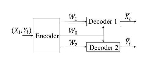
Fig. 1: Gray-Wyner source coding network.

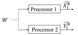
Fig. 2: The RV generators for Gray-Wyner source coding.

The paper is organized as follows: Section II presents the background of lossless and lossy compression using polar codes. The construction of polar codes for the lossless Gray-Wyner network is investigated in Section III. In Section IV, we construct polar codes for a DSBS for the lossy Gray-Wyner network, and show simulation results for different distortion regions. In Section V, we construct polar codes for a pair of Gaussian variables for the lossy Gray-Wyner network; then we extend the method to multiple Guassian sources. Finally, the paper is concluded in Section VI.

Notations: All random variables (RVs) are denoted by capital letters. $P_{X}$ denotes the probability distribution of a RV $X$ taking value $x$ in a set $\mathcal{X}$. $X_{1}^{N}$ denotes a vector $(X_{1},...,X_{N})$. For a set $\mathcal{I}$, $\mathcal{I}^{c}$ denotes its complement, and $|\mathcal{I}|$ denotes its cardinality. $X_{\mathcal{I}}$ denotes the subvector $\{X_{i}\}_{i\in\mathcal{I}}$. For an integer $N$, $[N]$ will be used to denote the set of all integers from $1$ to $N$. The information is measured in bits and $h(\cdot)$ denotes the binary entropy function.

II Polar Codes for Source Coding

II-A Polar Codes for Lossless Source Coding [15]

Let $X_{1}^{N}$ to be $N$ i.i.d. drawings of a RV $X$, where $X$ is a Bernoulli source with crossover probability $p$ (Ber($p$)). $N=2^{n}$ for any integer $n\geq 1$. The polarizing transformation is defined by

$$U_{1}^{N}\triangleq X_{1}^{N}G_{N},$$

where $G_{N}=G_{2}^{\otimes n}$ is the $n$-fold Kronecker product of matrix

$$G_{2}=\begin{bmatrix}1&0\\ 1&1\end{bmatrix}.$$

Fix $R>H(X)$ and let $\mathcal{F}$ denote the frozen set such that $|\mathcal{F}|=\left\lceil NR\right\rceil$ and $H(U_{i}|U_{1}^{i-1})\geq H(U_{j}|U_{1}^{j-1})$ for all $i\in\mathcal{F}$, $j\notin\mathcal{F}$. The information set is given by $\mathcal{I}=\mathcal{F}^{c}$.

The Successive Cancellation (SC) encoder introduced in [20] stores $u_{\mathcal{F}}$ and computes $\hat{u}_{\mathcal{I}}$, following the encoding rules (1) explained in Section II-B. If $\hat{u}_{i}\neq u_{i}$ for $i\in\mathcal{I}$, an estimation error occurs and the index $i$ needs to be announced to the decoder. The set of error indices is denoted by $T$. The encoder outputs $(u_{\mathcal{F}},T)$. The decoder puts $\hat{u}_{i}=u_{i}$ for $i\in\mathcal{F}$, then estimates $u_{\mathcal{I}}$ using the same rule to the SC encoder (1). If $i\in T$, the decision is flipped. In the end, the decoder outputs $\hat{x}_{1}^{N}=\hat{u}_{1}^{N}G_{N}$. It has been shown in [20] that the error rate tends to zero for any rate $R>H(X)$.

Since the entropy $H(U_{i}|U_{1}^{i-1})$ is complicated to analyze when $N$ becomes very large, the Bhattacharyya parameter is often used. For source coding with side information, assume $(X,Y)\in\{0,1\}\times\mathcal{Y}$ be a pair of RVs. The Bhattacharyya parameter [21] is defined as

$$Z(X|Y)\triangleq 2\sum_{y}P_{Y}(y)\sqrt{P_{X|Y}(0|y)P_{X|Y}(1|y)}.$$

$Z(X|Y)$ and $H(X|Y)$ are related by [21, Proposition 2], which indicates that $H(X|Y)$ is near $0$ or $1$ if and only if $Z(X|Y)$ is near $0$ or $1$, respectively. Hence, the parameters $\{H(U_{i}|U_{1}^{i-1})\}_{1}^{N}$ and $\{Z(U_{i}|U_{1}^{i-1})\}_{1}^{N}$ polarize simultaneously.

Furthermore, [17, 22] show that the Bhattacharyya parameter of an asymmetric channel can be equalized to the one in the symmetric case. Therefore we can apply the known results in constructing polar codes for symmetric channels [23] to that for asymmetric channels.

II-B Polar Codes for Lossy Source Coding [15, 17]

In this subsection, we discuss the lossy source coding for a nonuniform source. We model the source as a sequence of i.i.d. realizations of a RV $Y\in\mathcal{Y}$. $\mathcal{X}$ denotes the reconstruction space. Denote the distortion function by $\text{d}:\mathcal{Y}\times\mathcal{X}\rightarrow\mathbb{R}_{+}$. The rate-distortion function is given by

$$R(D)=\min_{\mathtt{\mathsf{E_{XY}}}[d(Y,X)]\leq D}I(X,Y).$$

Similarly to lossless source coding, $U_{1}^{N}$ is defined as $U_{1}^{N}\triangleq X_{1}^{N}G_{N}$. The frozen set $\mathcal{I}^{c}$ can be identified by

$$Z(U_{i}|U_{1}^{i-1},Y_{1}^{N})\geq 1-2^{-N^{\beta}}\textrm{ or }Z(U_{i}|U_{1}^{i-1})\leq 2^{-N^{\beta}}$$

for all $i\in\mathcal{I}^{c}$. As a result, the information set satisfies $|\mathcal{I}|=NR$, where $R$ is the encoding rate. [17] has shown that such an information set exists if $R>I(X,Y)=R(D)$, $\beta<1/2$ and $N$ is sufficiently large.

Once the indices of the information set and the frozen set are identified, the encoder determines $u_{1}^{N}$ from a given source sequence $y_{1}^{N}$ by the rules

$$u_{i}=\begin{cases}0,&\textrm{with probability }P_{U_{i}|U_{1}^{i-1},Y_{1}^{N}}(0|u_{1}^{i-1},y_{1}^{N})\\ 1,&\textrm{with probability }P_{U_{i}|U_{1}^{i-1},Y_{1}^{N}}(1|u_{1}^{i-1},y_{1}^{N})\end{cases}$$ (1)

for $i\in\mathcal{I}$ and

$$u_{i}=\begin{cases}\bar{u}_{i},&\textrm{if }Z(U_{i}|U_{1}^{i-1},Y_{1}^{N})\geq 1-2^{-N^{\beta}}\\ \arg\max_{u}P_{U_{i}|U_{1}^{i-1}}(u|u_{1}^{i-1}),&\textrm{if }Z(U_{i}|U_{1}^{i-1})\leq 2^{-N^{\beta}}\end{cases}$$ (2)

for $i\in\mathcal{I}^{c}$. $\bar{u}_{i}$ is determined beforehand uniformly from $\{0,1\}$, and shared between the encoder and the decoder. Although the encoding scheme in [17, Theorem 4] is proved using a randomized map shared between the encoder and the decoder, the alternative rule (2) in our scheme has also been proposed in [17] and further proved in [18]. In the end, the encoder sends $u_{\mathcal{I}}$ to the decoder and the decoder outputs the reconstructed sequence $x_{1}^{N}=u_{1}^{N}G_{N}$.

Finally, it has been proved in [17] that the average distortion between the source and the reconstruction can be equivalent to $D+O(2^{-N^{\beta^{\prime}}})$ where $\beta^{\prime}<\beta<1/2$. Notice that the above construction is also applicable to symmetric sources, with the index set $\{i:Z(U_{i}|U_{1}^{i-1})\leq 2^{-N^{\beta}}\}=\textrm{\O}$. Additionally, the rule (1) reduces to that of lossless coding in the absence of $y_{1}^{N}$.

III Polar Codes for Lossless Gray-Wyner Coding

In this section, we use the DSBS as an example to show that polar codes are able to achieve the rate region of the Gray-Wyner network in the lossless case. Consider the lossless coding model using Wyner’s first approach depicted in Fig. 1. Define the measurement of distortions as

$$d^{N}(y_{1}^{N},x_{1}^{N})\triangleq\sum_{i=1}^{N}d(y_{i},x_{i}),$$

where $d(y,x)$ denotes Hamming distance for discrete RVs or Euclidean distance for continuous RVs. Following that, we give a formal definition to this model.

Definition 1.

An $(N,M_{0},M_{1},M_{2})$ code for the lossless Gray-Wyner coding depicted in Fig. 1 is defined as follows:

An encoder is a mapping

$$f_{E}:\mathcal{X}^{N}\times\mathcal{Y}^{N}\rightarrow I_{M_{0}}\times I_{M_{1}}\times I_{M_{2}},$$

where $I_{M_{i}}=\{0,1,2,\ldots,M_{i}-1\}$ for $i=0,1,2$.

A decoder is a pair of mappings

$$f_{D}^{(X)}:I_{M_{0}}\times I_{M_{1}}\rightarrow\mathcal{X}^{N}$$

$$f_{D}^{(Y)}:I_{M_{0}}\times I_{M_{2}}\rightarrow\mathcal{Y}^{N}.$$

Let $f_{E}(X_{1}^{N},Y_{1}^{N})=(W_{0},W_{1},W_{2})$, then

$$\hat{X}_{1}^{N}=f_{D}^{(X)}(W_{0},W_{1})$$

$$\hat{Y}_{1}^{N}=f_{D}^{(Y)}(W_{0},W_{2}).$$

The average distortion between the inputs and outputs are $(\triangle_{X},\triangle_{Y})$, where

$$\triangle_{X}=\frac{1}{N}\mathsf{E}d^{N}(X_{1}^{N},\hat{X}_{1}^{N})$$

$$\triangle_{Y}=\frac{1}{N}\mathsf{E}d^{N}(Y_{1}^{N},\hat{Y}_{1}^{N}).$$

The achievable rate region of an $(N,M_{0},M_{1},M_{2})$ code is defined as follows.

Definition 2.

For lossless coding, a triple $(R_{0},R_{1},R_{2})$ is said to be $\mathit{achievable}$ if there exists an $(N,M_{0},M_{1},M_{2})$ code with $M_{i}\leq 2^{N(R_{i}+\epsilon)}$, $i=0,1,2$ and $\bigtriangleup=\max(\triangle_{X},\triangle_{Y})\leq\epsilon$, for arbitrary $\epsilon>0$ and sufficiently large $N$. Denote $\mathcal{R}$ as the set of achievable rate.

Theorem 3.

([9, Theorem 2]) If $(R_{0}$,$R_{1}$,$R_{2})\in\mathcal{R}$, then

$$\begin{cases}R_{0}+R_{1}+R_{2}\geq H(X,Y)\\ R_{0}+R_{1}\geq H(X)\\ R_{0}+R_{2}\geq H(Y).\end{cases}$$

Let us consider a DSBS $(X,Y)$, where $\mathcal{X}=\mathcal{Y}=\{0,1\}$ and $Y=X\oplus Z$, $Z\sim\textrm{Ber}(a_{0})$. In this case, $H(X,Y)=1+h(a_{0})$, $H(X)=H(Y)=1$. It has been shown in [4] that the common information of DSBS is $C(X,Y)=1+h(a_{0})-2h(a_{1})$, where $a_{1}=\frac{1}{2}-\frac{1}{2}(1-2a_{0})^{1/2}$. This model can be considered a cascade of two Binary Symmetric Channels (BSCs) with the same crossover probability $a_{1}$. The cascaded channel is equivalent to a single BSC($a_{0}$). It was shown in [4] that the common information $C(X,Y)$ can be achieved when $W$ is an intermediate RV as depicted in Fig. 3 (a).

Fig. 3: Test channel for (a) Wyner’s common information for DSBS source, where $a_{0}=a_{1}*a_{1}$. (b) Line AG and lossy Gray-Wyner coding, where $a_{1}=D_{1}*D_{2}$. (C) Line GB. ($a*b\triangleq a(1-b)+b(1-a)$).

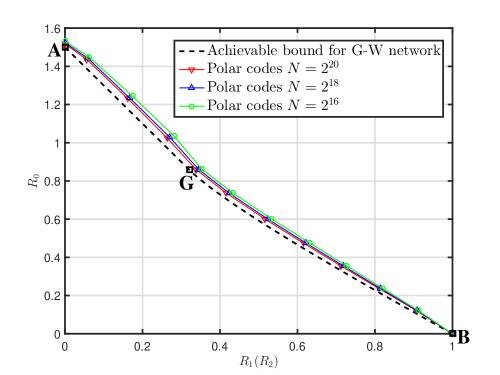
Fig. 4: Simulation performance of polar codes for Gray-Wyner lossless coding when $a_{0}=0.11$ and $N=2^{16},2^{18},2^{20}$. The performance loss between AG is due to the nonuniform source coding.

III-A Polar codes for Pangloss bound

Theorem 3 indicates a fact that the Gray-Wyner network defined in Definition 2 cannot perform better than the situation where the receivers can collaborate. This situation is referred to as the Pangloss plane [9], where the triple $(R_{0},R_{1},R_{2})$ satisfies

$$\sum_{i=0}^{2}R_{i}=H(X,Y).$$

The dashed line AG in Fig. 4 is the Pangloss bound for the lossless Gray-Wyner problem. Point A refers to the case where only the common branch is used. Therefore the problem is the same to the joint compression for source $(X,Y)$ when $(R_{0},R_{1},R_{2})=(H(X,Y),0,0)$. Point G refers to the case where $R_{0}$ is the smallest rate that achieves lossless compression for source $(X,Y)$ when the total rate equals $H(X,Y)$. In other words, $R_{0}$ achieves Wyner’s common information $C(X,Y)$ at point G and $(R_{0},R_{1},R_{2})=(1+h(a_{0})-2h(a_{1}),h(a_{1}),h(a_{1}))$. Next we demonstrate how to achieve the Pangloss bound using polar codes without time-sharing.

• Point A:

This point can be trivially achieved, since

$$H(X,Y)=H(X)+H(Y|X)=H(X)+H(Z).$$

In this case, $X$ does not need to be compressed. Encoder sends $x_{1}^{N}$ and compresses $z_{1}^{N}=x_{1}^{N}\oplus y_{1}^{N}$ as introduced in Section II-A. Decoders 1 and 2 reconstruct $\hat{x}_{1}^{N}$ and $\hat{z}_{1}^{N}$ with error probability tending to zero when $N$ is sufficiently large. Then $\hat{y}_{1}^{N}=\hat{x}_{1}^{N}\oplus\hat{z}_{1}^{N}$. Due to symmetry, the role of source $X$ and $Y$ can be exchanged.

• Point G:

Firstly we extract the common information from source $(X_{1}^{N},Y_{1}^{N})$. Since

$$R_{0}\geq I(W;XY)=1+h(a_{0})-2h(a_{1}),$$

the encoder applies lossy compression to the joint sources $(x_{1}^{N},y_{1}^{N})$ as introduced in Section II-B with reconstruction $w_{1}^{N}$. Differently from traditional lossy compression with a single source, the test channel for the joint sources is

$$P_{XY|W}(xy|w)=P_{X|W}(x|w)P_{Y|W}(y|w).$$

In this way, the average distortion between $w_{1}^{N}$ and $x_{1}^{N}$ or $w_{1}^{N}$ and $y_{1}^{N}$ will tend to $a_{1}$ simultaneously as $N$ increases. Hence the lossy-compressed sequence $u_{\mathcal{I}}$ is the common message and is sent to both decoders, where $|\mathcal{I}|\geq(1+h(a_{0})-2h(a_{1}))N$. Since

$$H(X|W)=H(Y|W)=h(a_{1}),$$

we apply lossless compression to source $x_{1}^{N}$ together with $w_{1}^{N}$ as side information and send the lossless compressed sequence privately to Decoder 1. Symmetrically, source $Y$ is operated in the same way.

At the decoder side, both decoders reconstruct $w_{1}^{N}$ from $u_{\mathcal{I}}$ by the lossy decoding rule introduced in Section II-B. Decoder 1 receives the compressed sequence from its private branch and derives a reconstructed sequence $\hat{z}_{1}^{N}$. Then the source can be reconstructed as $\hat{x}_{1}^{N}=\hat{z}_{1}^{N}\oplus w_{1}^{N}$. Decoder 2 operates in the same way. Therefore, $X$ and $Y$ can be reconstructed with error rate tending to zeros when $N$ is sufficiently large. Notice that a similar method was also given in [19].

• Points on dashed line AG:

On this line, the common branch carries more information than point G. In order to show how much additional amount of information to be sent over the common branch, we keep the relation that $X-W-Y$ is a Markov chain. Now, if we move the intermediate RV $W$ closer to sources $(X,Y)$, there will be two new RVs $(X^{\prime},Y^{\prime})$ between the source and common RV $W$ correspondingly. Hence we assume that the test channel is a BSC($d_{1}$) between $X$ ($Y$) and $X^{\prime}$ ($Y^{\prime}$), and a BSC($d_{2}$) between $W$ and $(X^{\prime}$,$Y^{\prime})$ where $0\leq d_{1},d_{2}\leq a_{1}$. This test channel is depicted in Fig. 3 (b). Therefore,

$$X-X^{\prime}-W-Y^{\prime}-Y$$

forms a Markov chain.

In this case, the rate of the common branch is

$$R_{0} \geq I(X^{\prime}Y^{\prime};XY)$$

$$=I(X^{\prime}Y^{\prime}W;XY)$$

$$=I(XY;W)+I(X^{\prime};X|W)+I(Y^{\prime};Y|W)$$

$$=1-2h(d_{1})+h(a_{0}).$$

Instead of extracting the common RV $W$ over the common branch, decoders can reconstruct $(X^{\prime},Y^{\prime})$ and retrieve more information from the common branch. This is because $(X^{\prime},Y^{\prime})$ is closer to $(X,Y)$ than $W$ in the Markov chain. Hence, both sources can be losslessly reconstructed by applying lossless compression to sources $(X,Y)$ with side information $(X^{\prime},Y^{\prime})$. Therefore the rate of the private branches is

$$R_{1}=R_{2}\geq H(X|X^{\prime})=H(Y|Y^{\prime})=h(d_{1}).$$

Next we show a construction using polar codes that achieves the rate bound. Similarly to point G, we can firstly retrieve the common message $w_{1}^{N}$ by applying lossy compression to joint source sequences $(x_{1}^{N},y_{1}^{N})$. The compressed rate approaches $1+h(a_{0})-2h(a_{1})$. Due to that $Z_{1}=X\oplus W$ is a Ber($a_{1}$) source, the encoder applies lossy compression to the nonuniform source realizations $x_{1}^{N}\oplus w_{1}^{N}$ with distortion $d_{1}$ as introduced in Section II-B. We operate the same to source $Y$. Therefore, the additional rate approaches $2(h(a_{1})-h(d_{1}))$ when $N$ is sufficiently large. For the private branches, the encoder firstly reconstructs $X^{\prime}$ and $Y^{\prime}$. Then the encoder applies lossless compression to source $X\oplus X^{\prime}$ and $Y\oplus Y^{\prime}$ with rate approaching $h(d_{1})$. It is known that polar codes are optimal for lossy and lossless compression [17, 21]. Therefore, the average distortion of sources $(X_{1}^{N},Y_{1}^{N})$ approaches zero when $N$ is sufficiently large.

III-B Polar codes for $R_{0}<C(X,Y)$ (Curve GB)

In this part, we show how to achieve the dashed curve GB in Fig. 4 using polar codes. From Theorem 3, the lower boundary of $\mathcal{R}$ should lie above the lines

$$\begin{cases}R_{0}+2R_{1}=1+h(a_{0})\\ R_{0}+R_{1}=1.\end{cases}$$

In the preceding subsection, we have shown constructions to achieve this lower boundary of $\mathcal{R}$, called Pangloss bound, when $R_{0}\geq C(X,Y)$ (e.g. dashed line AG in Fig. 4). However the lower boundary of $\mathcal{R}$ remains unknown when $R_{0}<C(X,Y)$. To the best of our knowledge, the tightest lower boundary was given in [9] for the case as follows:

Consider a degradation applied on the common RV $W$, where $W$ is considered the input to BSC($\rho$) with output $W^{\prime}$ as shown in Fig. 3 (C). As a result,

$$(X,Y)-W-W^{\prime}$$

forms a Markov chain and $a_{1}\leq\beta=a_{1}*\rho\leq 1/2$.

From this Markov chain, the transition probability reads

$$P_{XY|W^{\prime}}(x,y|w^{\prime}) =\sum_{w\in\mathcal{W}}P_{W|W^{\prime}}(w|w^{\prime})P_{X|W}(x|w)P_{Y|W}(y|w).$$ (3)

Then the triple $(R_{0},R_{1},R_{2})\in\mathcal{R}$ satisfies

$$\begin{cases}R_{0}=I(W^{\prime};XY)=(1-a_{0})(1-h(\frac{\beta-0.5a_{0}}{1-a_{0}}))\\ R_{1}=R_{2}=H(X|W^{\prime})=H(Y|W^{\prime})=h(\beta).\end{cases}$$ (4)

As $\beta\in[a_{1},\frac{1}{2}]$, the family of rate triples can generate the dashed curve GB in Fig. 4. In fact, achieving the triple in (4) is quite similar to achieving the rate bound for point G using polar codes. Firstly we apply lossy compression to joint sources $(X_{1}^{N},Y_{1}^{N})$ with distortion $\beta$ and derive reconstruction $W^{\prime}$. The test channel used in lossy compression is specified in (3), which is the major difference from the construction of point G. Next, send the compressed sequence over the common branch. After that, we apply lossless compression to source $X$ and $Y$ with $W^{\prime}$ as side information, and send the compressed sequences through private branches to decoder 1 and 2 accordingly. Alternatively we can derive the common RV $W$ by lossy compression of $(X,Y)$. Afterwards, we apply symmetric lossy compression to $W$ with distortion $\rho$ to obtain $W^{\prime}$. Finally, it is trivial to achieve point $B$ when $R_{1}=R_{2}=1$ and $R_{0}=0$.

Together with the result from III-A, all points from point A to B along the dashed line in Fig. 4 can be achieved by polar codes. Moreover, the above models can be extended to achieving the lower boundary of more general binary-correlated sources mentioned in [24, Theorem 3].

IV Lossy Gray-Wyner Coding for a DSBS

In this section, we show how to achieve the lossy common information $C\left(\triangle_{1},\triangle_{2}\right)$, which is defined as the smallest common rate $R_{0}$, such that the total rate meets the rate-distortion bound. Based on Definition 1, we define the lossy Gray-Wyner coding as follows:

The rate-distortion function for source $(X,Y)$ is

$$R_{XY}\left(\triangle_{1},\triangle_{2}\right)=\min_{P_{X^{\prime}Y^{\prime}|XY}(x^{\prime}y^{\prime}|xy):\mathsf{E}d(X^{\prime},X)\leq\triangle_{1},\mathsf{E}d(Y^{\prime},Y)\leq\triangle_{2}}I(X^{\prime},Y^{\prime};X,Y),$$

where the minimum is taken over all test channels $P_{X^{\prime}Y^{\prime}|XY}(x^{\prime}y^{\prime}|xy)$ such that $\mathsf{E}d(X^{\prime},X)\leq\triangle_{1}$ and $\mathsf{E}d(Y^{\prime},Y)\leq\triangle_{2}$.

Definition 4.

For any $\triangle_{1},\triangle_{2}\geq 0$, a number $R_{0}$ is said to be $\left(\triangle_{1},\triangle_{2}\right)\mathit{-achivable}$ if for any $\varepsilon>0$ we can find a sufficiently large $N$ such that there exists a $(N,M_{0},M_{1},M_{2})$ code with

$$M_{0} \leq 2^{NR_{0}},$$

$$\sum_{i=0}^{2}\frac{1}{N}\log M_{i} \leq R_{XY}\left(\triangle_{1},\triangle_{2}\right)+\varepsilon,$$

$$\triangle_{X} \leq\triangle_{1}+\varepsilon,$$

$$\triangle_{Y} \leq\triangle_{2}+\varepsilon.$$

Then $C\left(\triangle_{1},\triangle_{2}\right)$ is defined as the infimum of all $R_{0}$ that is $\left(\triangle_{1},\triangle_{2}\right)$-achievable.

To avoid ambiguity, we refer $C\left(\triangle_{1},\triangle_{2}\right)$ to lossy common information and $C\left(X,Y\right)$ to common information or Wyner’s common information in this section.

The authors gave a characterization of $C\left(\triangle_{1},\triangle_{2}\right)$ in [10] as follows:

Definition 5.

Given a pair of joint sources $\left(X,Y\right)\sim P_{XY}(x,y)$, for any $\triangle_{1},\triangle_{2}\geq 0$, the lossy common information reads

$$C\left(\triangle_{1},\triangle_{2}\right)=\inf I\left(X,Y;W\right),$$

where the infimum is taken over all joint distributions for $X$, $Y$, $X^{\prime}$, $Y^{\prime}$, $W$ such that

$$X^{\prime}-W-Y^{\prime},$$ (5)

$$\left(X,Y\right)-\left(X^{\prime},Y^{\prime}\right)-W,$$

and $\left(X^{\prime},Y^{\prime}\right)$ achieves $R_{XY}\left(\triangle_{1},\triangle_{2}\right)$.

Notice that this is a more generalized characterization, comparing with that for lossless Gray-Wyner network where $X$ and $Y$ are independent given $W$.

Following the above definition, we consider the same DSBS $\left(X,Y\right)$ to the previous section. The joint distribution of $\left(X,Y\right)$ is given by

$$P_{X,Y}\left(x,y\right)=\begin{cases}\frac{1}{2}\left(1-a_{0}\right),&\textrm{if}\textrm{ }x=y\\ \frac{1}{2}a_{0},&\textrm{otherwise},\end{cases}$$

where $a_{0}\in\left[0,\frac{1}{2}\right]$. Let $a_{0}=2a_{1}\left(1-a_{1}\right)$ and $a_{1}\in\left[0,\frac{1}{2}\right]$.

The lossy common information for $\left(X,Y\right)$ has been given by [1]

$$C\left(\triangle_{1},\triangle_{2}\right)=\begin{cases}C\left(X,Y\right)&\left(\triangle_{1},\triangle_{2}\right)\in\varepsilon_{10},\\ R_{XY}\left(\triangle_{1},\triangle_{2}\right)&\left(\triangle_{1},\triangle_{2}\right)\in\varepsilon_{2}\cup\varepsilon_{3}\\ 0&\left(\triangle_{1},\triangle_{2}\right)\geq\left(\frac{1}{2},\frac{1}{2}\right),\end{cases},$$

$$C\left(X,Y\right)\leq C\left(\triangle_{1},\triangle_{2}\right)\leq R_{XY}\left(\triangle_{1},\triangle_{2}\right),\textrm{ }\textrm{ }\textrm{ }\left(\triangle_{1},\triangle_{2}\right)\in\varepsilon_{11},$$

where

$$\varepsilon_{10} =\left\{\left(\triangle_{1},\triangle_{2}\right):0\leq\triangle_{i}\leq a_{1},\textrm{ }i=1,2\right\},$$

$$\varepsilon_{11} =\varepsilon_{10}^{c}\cap\left\{\left(\triangle_{1},\triangle_{2}\right):\triangle_{1}+\triangle_{2}-2\triangle_{1}\triangle_{2}\leq a_{0}\right\},$$

$$\varepsilon_{2} =\varepsilon_{10}^{c}\cap\varepsilon_{11}^{c}\cap\left\{\left(\triangle_{1},\triangle_{2}\right):\max\left\{\frac{\triangle_{1}-\triangle_{2}}{1-2\triangle_{2}},\frac{\triangle_{2}-\triangle_{1}}{1-2\triangle_{1}}\right\}\leq a_{0}\right\},$$

$$\varepsilon_{3} =\varepsilon_{10}^{c}\cap\varepsilon_{11}^{c}\cap\varepsilon_{2}^{c}\cap\left\{\left(\triangle_{1},\triangle_{2}\right):\triangle_{i}\leq\frac{1}{2},\textrm{ }i=1,2\right\}.$$

The relations among these four regions are depicted in Fig. 5. The joint rate distortion function of the DSBS $\left(X,Y\right)$ is given by [25]

$$R_{XY}\left(\triangle_{1},\triangle_{2}\right)=\begin{cases}1+h\left(a_{0}\right)-h\left(\triangle_{1}\right)-h\left(\triangle_{2}\right),&\left(\triangle_{1},\triangle_{2}\right)\in\varepsilon_{1},\\ 1-\left(1-a_{0}\right)h\left(\frac{\triangle_{1}+\triangle_{2}-a_{0}}{2\left(1-a_{0}\right)}\right)-a_{0}h\left(\frac{\triangle_{1}-\triangle_{2}+a_{0}}{2a_{0}}\right),&\left(\triangle_{1},\triangle_{2}\right)\in\varepsilon_{2},\\ 1-h\left(\min\left\{\triangle_{1},\triangle_{2}\right\}\right),&\left(\triangle_{1},\triangle_{2}\right)\in\varepsilon_{3},\end{cases}$$

where $\varepsilon_{1}=\varepsilon_{10}\cup\varepsilon_{11}$.

Fig. 5: The distortion regions for DSBS when $a_{0}=0.11$.

First, we provide an operational meaning of the region $\left(\triangle_{1},\triangle_{2}\right)\in\varepsilon_{10}$, where $C\left(\triangle_{1},\triangle_{2}\right)=C(X,Y)$.

The relation between lossy and lossless Gray-Wyner coding is not difficult to find if we recall the construction of polar codes for the line AG in Section III-A. We apply the same test channel where $X-X^{\prime}-W-Y^{\prime}-Y$ forms a Markov chain depicted by Fig. 3 (b). The rate of the shared branch in lossless Gray-Wyner coding reads

$$I(X^{\prime}Y^{\prime};XY)=I(XY;W)+I(X^{\prime};X|W)+I(Y^{\prime};Y|W).$$

Thus we shall send all of the three sub-sequences over the shared branch.

Notice that if we consider $(X^{\prime},Y^{\prime})$ the output of the decoders, the above rate is sufficient for lossy Gray-Wyner coding. In the lossy case, we only require to recover the sources $(X,Y)$ with distortions $\left(\triangle_{1},\triangle_{2}\right)$. Therefore, we consider the intermediate RVs $(X^{\prime},Y^{\prime})$ as the reconstruction RVs.

Similar to the case in Section III-A, we only consider the plane in the $\left(R_{0},R_{1},R_{2}\right)$ space where $R_{1}=R_{2}$ and $\triangle_{1}=\triangle_{2}=\triangle$. The encoder applies the same lossy compression as that for line AG to extract $W$, and sends it on the shared branch with rate $R_{0}\geq I(XY;W)$. Next, the encoder applies lossy compression to the nonuniform source $X\oplus W$ with distortion $\triangle$ where $a_{1}=d_{2}*\triangle$. To achieve $\triangle_{1}=\triangle_{2}=\triangle$, the additional rate we should send is $I(X^{\prime};X|W)$ and $I(Y^{\prime};Y|W)$ over either private branches or the shared branch. Then the distortion between $X(Y)$ and $X^{\prime}(Y^{\prime})$ tends to $\triangle$ when $N$ is sufficiently large. As a result, the total rate

$$\sum_{i=0}^{2}R_{i}\rightarrow I(X^{\prime}Y^{\prime};XY) =1+h(a_{0})-2h(\triangle)=R_{XY}(\triangle,\triangle),$$

where $0\leq\triangle\leq a_{1}$. This indicates that the lossy Pangloss bound [9] can be achieved as long as $0\leq\triangle\leq a_{1}$ and $C\left(\triangle,\triangle\right)=C\left(X,Y\right)$.

For $\left(\triangle_{1},\triangle_{2}\right)\in\varepsilon_{2}\cup\varepsilon_{3}$ , the lossy common information exactly equals the optimal rate for a certain distortion pair for the joint DSBS. This means that all the messages should be sent over the shared branch to achieve the desired distortion $\left(\triangle_{1},\triangle_{2}\right)\in\varepsilon_{2}\cup\varepsilon_{3}$.

We then construct polar codes to extract the lossy common information for $\left(\triangle_{1},\triangle_{2}\right)\in\varepsilon_{2}$. Fortunately the backward test channel that achieves $R_{XY}\left(\triangle_{1},\triangle_{2}\right)$ has been given by [25]

$$\begin{cases}X=X^{\prime}+Z_{1}\\ Y=Y^{\prime}+Z_{2},\end{cases}$$

where $\left[X^{\prime},Y^{\prime}\right]^{\mathrm{T}}$ and $\left[Z_{1},Z_{2}\right]^{\mathrm{T}}$ are vectors contained binary RVs ($\cdot^{\mathrm{T}}$ stands for matrix transpose), where the two vectors are independent of each other. Additionally, the probability mass function are given by

$$P_{X^{\prime},Y^{\prime}}(x^{\prime},y^{\prime})=\begin{bmatrix}\frac{1}{2}&0\\ 0&\frac{1}{2}\end{bmatrix},\textrm{ }\textrm{ }\textrm{ }$$

$$P_{Z_{1},Z_{2}}(z_{1},z_{2})=\frac{1}{2}\begin{bmatrix}2-a_{0}-\triangle_{1}-\triangle_{2}&\triangle_{2}-\triangle_{1}+a_{0}\\ \triangle_{1}-\triangle_{2}+a_{0}&\triangle_{1}+\triangle_{2}-a_{0}\end{bmatrix}.$$

From the joint probability $P_{X^{\prime},Y^{\prime}}(x^{\prime},y^{\prime})$, it is trivial that the condition for $\left(X^{\prime},Y^{\prime}\right)$ to achieve $R_{XY}\left(\triangle_{1},\triangle_{2}\right)$ is

$$X^{\prime}=Y^{\prime}.$$

For simplicity, we assign a binary RV $W$ such that $W=X^{\prime}=Y^{\prime}$.

Similar to the code construction of Curve GB, we design polar codes for performing the lossy compression that generates the reconstruction $W$ on the joint sources $\left(X,Y\right)$. The transition probability of the test channel is given by

$$\begin{cases}\begin{aligned} P_{XY|W}(0,0|1)&=P_{XY|W}(1,1|0)=P_{Z_{1}Z_{2}}(1,1)=\frac{1}{2}\left(\triangle_{1}+\triangle_{2}-a_{0}\right),\end{aligned}\\ \begin{aligned} P_{XY|W}(0,1|1)&=P_{XY|W}(1,0|0)=P_{Z_{1}Z_{2}}(1,0)=\frac{1}{2}\left(\triangle_{1}-\triangle_{2}+a_{0}\right),\end{aligned}\\ \begin{aligned} P_{XY|W}(1,0|1)&=P_{XY|W}(0,1|0)=P_{Z_{1}Z_{2}}(0,1)=\frac{1}{2}\left(\triangle_{2}-\triangle_{1}+a_{0}\right),\end{aligned}\\ \begin{aligned} P_{XY|W}(1,1|1)&=P_{XY|W}(0,0|0)=P_{Z_{1}Z_{2}}(0,0)=\frac{1}{2}\left(2-a_{0}-\triangle_{1}-\triangle_{2}\right).\end{aligned}\end{cases}$$

Notice that the test channel is asymmetric, which is different from the symmetric test channel $\left(\ref{eq:Transition probability}\right)$ for Curve GB. Therefore we should design polar codes for the lossy compression with asymmetric test channels, as mentioned in Section II-B. After that, we send the compressed sequence through the shared branch to the two decoders. The simulation performance for $\left(\triangle_{1},\triangle_{2}\right)\in\varepsilon_{2}$ is shown in Fig. 6. The dashed line is the achievable bound $R_{XY}\left(\triangle_{1},\triangle_{2}\right)$ when $\left(\triangle_{1},\triangle_{2}\right)\in\varepsilon_{2}$ and $\triangle_{1}=\triangle_{2}$. As for the lines of simulation results with $N=2^{12},2^{14},2^{16},2^{18},2^{20}$, the horizontal axis refers to the average distortion between the practical $\triangle_{1}$ and $\triangle_{2}$. In fact, the practical $\triangle_{1}$ and $\triangle_{2}$ tend to be very close to each other when the number of simulation rounds is large.

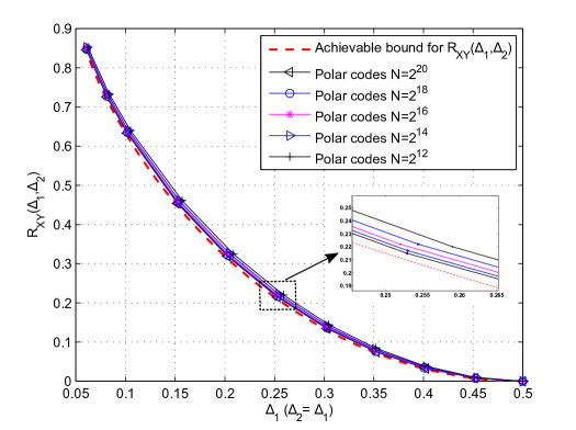
Fig. 6: Simulation performance for polar codes for Gray-Wyner lossy coding when $\left(\triangle_{1},\triangle_{2}\right)\in\varepsilon_{2}$ , $\triangle_{1}=\triangle_{2}$ and $a_{0}=0.11$. The blocklength of polar codes is given by $N=2^{12},2^{14},2^{16},2^{18},2^{20}.$

Region $\varepsilon_{3}$ is a degenerate region in the sense that, for example, if $a_{0}<\frac{\triangle_{2}-\triangle_{1}}{1-2\triangle_{1}}$ and $\triangle_{i}\leq\frac{1}{2}$, $i=1,2$, we have $R_{XY}\left(\triangle_{1},\triangle_{2}\right)=R_{X}\left(\triangle_{1}\right)$. This implies that the optimal code strategy is to ignore $Y$ and optimally compress $X$. Hence, $Y^{\prime}$ can be estimated from $X^{\prime}$ with distortion less than $\triangle_{2}$. The case when $a_{0}<\frac{\triangle_{1}-\triangle_{2}}{1-2\triangle_{2}}$ can be solved similarly. Therefore, polar codes can be designed for the lossy compression of a single source in this region.

So far, we have constructed polar codes to extract the lossy common information $C\left(\triangle_{1},\triangle_{2}\right)$ in the entire distortion region except for region $\varepsilon_{11}$. From [1], we know that $C\left(X,Y\right)\leq C\left(\triangle_{1},\triangle_{2}\right)$ for $\left(\triangle_{1},\triangle_{2}\right)\in\varepsilon_{11}$; however, the exact value of the lossy common information in region $\varepsilon_{11}$ remains unknown.

V Lossy Gray-Wyner Coding for Gaussian RVs

Apart from the DSBS case addressed in the previous section, the lossy common information has also been generalized to two Gaussian RVs in [1]. In this section, we propose a coding scheme to extract the lossy common information of a pair of joint Gaussian sources using polar lattices.

Let $X$, $Y$ be two Gaussian RVs with zero mean and covariance matrix

$$K_{2}=\begin{bmatrix}1&\rho\\ \rho&1\end{bmatrix},$$

with $0<\rho<1$. The lossy common information for $\left(X,Y\right)$ has been given by [1]

$$C\left(\triangle_{1},\triangle_{2}\right)=\begin{cases}C\left(X,Y\right)&\left(\triangle_{1},\triangle_{2}\right)\in\varepsilon_{10},\\ R_{XY}\left(\triangle_{1},\triangle_{2}\right)&\left(\triangle_{1},\triangle_{2}\right)\in\varepsilon_{2}\cup\varepsilon_{3}\\ 0&\left(\triangle_{1},\triangle_{2}\right)\geq\left(1,1\right),\end{cases},$$ (6)

$$C\left(X,Y\right)\leq C\left(\triangle_{1},\triangle_{2}\right)\leq R_{XY}\left(\triangle_{1},\triangle_{2}\right),\textrm{ }\textrm{ }\textrm{ }\left(\triangle_{1},\triangle_{2}\right)\in\varepsilon_{11},$$

where

$$\varepsilon_{10} =\left\{\left(\triangle_{1},\triangle_{2}\right):0\leq\triangle_{i}\leq 1-\rho,\textrm{ }i=1,2\right\},$$

$$\varepsilon_{11} =\varepsilon_{10}^{c}\cap\left\{\left(\triangle_{1},\triangle_{2}\right):\triangle_{1}+\triangle_{2}-\triangle_{1}\triangle_{2}\leq 1-\rho^{2}\right\},$$

$$\varepsilon_{2} =\varepsilon_{10}^{c}\cap\varepsilon_{11}^{c}\cap\left\{\left(\triangle_{1},\triangle_{2}\right):\min\left\{\frac{1-\triangle_{1}}{1-\triangle_{2}},\frac{1-\triangle_{2}}{1-\triangle_{1}}\right\}\leq\rho^{2}\right\},$$

$$\varepsilon_{3} =\varepsilon_{10}^{c}\cap\varepsilon_{11}^{c}\cap\varepsilon_{2}^{c}\cap\left\{\left(\triangle_{1},\triangle_{2}\right):\triangle_{i}\leq 1,\textrm{ }i=1,2\right\}.$$

These distortion regions are illustrated in Fig. 7. The joint rate-distortion function of the Gaussian sources $\left(X,Y\right)$ described above is given by [25]

$$R_{XY}\left(\triangle_{1},\triangle_{2}\right)=\begin{cases}\frac{1}{2}\log\frac{1-\rho^{2}}{\triangle_{1}\triangle_{2}},&\left(\triangle_{1},\triangle_{2}\right)\in\varepsilon_{1},\\ \frac{1}{2}\log\frac{1-\rho^{2}}{\triangle_{1}\triangle_{2}-\left(\rho-\sqrt{\left(1-\triangle_{1}\right)\left(1-\triangle_{2}\right)}\right)^{2}},&\left(\triangle_{1},\triangle_{2}\right)\in\varepsilon_{2},\\ \frac{1}{2}\log\frac{1}{\min\left\{\triangle_{1},\triangle_{2}\right\}},&\left(\triangle_{1},\triangle_{2}\right)\in\varepsilon_{3},\end{cases}$$

where $\varepsilon_{1}=\varepsilon_{10}\cup\varepsilon_{11}$.

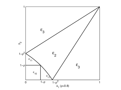
Fig. 7: The distortion regions for bivariate Gaussian RVs when $\rho=0.8$.

Notice that the relation $C\left(\triangle,\triangle\right)=C\left(X,Y\right)$ for $\triangle\leq 1-\rho$ was firstly proposed in [26]. Then it has been extended to the case where $\triangle_{1}\neq\triangle_{2}$ as presented in (6).

Next we show how to extract the lossy common information that lies in each of the distortion regions $\varepsilon_{10}$, $\varepsilon_{2}$ and $\varepsilon_{3}$. Notice that the characterizations of the common RV $W$ defined in (5) applies in $\varepsilon_{10}$, $\varepsilon_{2}$ and $\varepsilon_{3}$.

We propose a discretized version of $W$ to convey the lossy common information of two joint Gaussian RVs, according to Wyner’s second approach to the characterization of common information [4]. The discretized version of $W$ is obtained by the use of polar lattices [18, 22]. Some definitions that are necessary for our scheme are given as follows.

An $n$-dimensional full-rank lattice is a discrete subgroup of $\mathbb{R}^{n}$ which can be defined by

$$\Lambda=\{\lambda=\mathbf{B}z:\textrm{ }z\in\mathbb{Z}^{n}\},$$

where $\mathbf{B}$ is the $n\times n$ generator matrix. For $\sigma>0$ and $c\in\mathbb{R}^{n}$, the Gaussian distribution of variance $\sigma^{2}$ centered at $c$ is defined as

$$f_{\sigma,c}(x)=\frac{1}{(\sqrt{2\pi}\sigma)^{n}}e^{-\frac{\|x-c\|^{2}}{2\sigma^{2}}},\>\>x\in\mathbb{R}^{n}.$$

Let $f_{\sigma,0}(x)=f_{\sigma}(x)$ for short.

Define a $\Lambda$-periodic function

$$f_{\sigma,\Lambda}(x)=\sum\limits_{\lambda\in\Lambda}f_{\sigma,\lambda}(x)=\frac{1}{(\sqrt{2\pi}\sigma)^{n}}\sum\limits_{\lambda\in\Lambda}e^{-\frac{\|x-\lambda\|^{2}}{2\sigma^{2}}}.$$

We note that $f_{\sigma,\Lambda}(x)$ is a probability density function (PDF) if $x$ is restricted to the fundamental region $\mathcal{R}(\Lambda)$. It is actually the PDF of the $\Lambda$-aliased Gaussian noise [27].

The flatness factor of a lattice $\Lambda$ is defined as [27]

$$\epsilon_{\Lambda}(\sigma)\triangleq\max\limits_{x\in\mathcal{R}(\Lambda)}|V(\Lambda)f_{\sigma,\Lambda}(x)-1|,$$ (7)

where $V(\Lambda)=|\text{det}({B})|$ denotes the volume of a fundamental region of $\Lambda$. It can be interpreted as the maximum variation of $f_{\sigma,\Lambda}(x)$ with respect to the uniform distribution over a fundamental region of $\Lambda$.

We define the discrete Gaussian distribution over $\Lambda$ centered at $c$ as the discrete distribution taking values in $\lambda\in\Lambda$ as

$$D_{\Lambda,\sigma,c}(\lambda)=\frac{f_{\sigma,c}(\lambda)}{f_{\sigma,c}(\Lambda)},\;\forall\lambda\in\Lambda,$$

where $f_{\sigma,\mathrm{c}}(\Lambda)=\sum_{\lambda\in\Lambda}f_{\sigma,\mathrm{c}}(\lambda)$. For convenience, we write $D_{\Lambda,\sigma}=D_{\Lambda,\sigma,\mathrm{0}}$. It has been shown in [28] that lattice Gaussian distribution preserves many properties of the continuous Gaussian distribution when the flatness factor is negligible. To keep the notations simple, we always set $c=0$ and $n=1$ (one-dimensional lattice $\Lambda$) in this work.

In addition, the Kullback-Leibler divergence of continuous distributions $f_{X}$ and $f_{Y}$ is defined by

$$\mathbb{D}(f_{X}\|f_{Y})=\int_{\mathbb{R}}f_{X}(x)\log\frac{f_{X}(x)}{f_{Y}(x)}dx.$$

The variation distance is defined by

$$\mathbb{V}(f_{X}\|f_{Y})=\int_{\mathbb{R}}\left|f_{X}(x)-f_{Y}(x)\right|dx.$$

V-A Lossy Common Information for Region $\varepsilon_{10}$

For $\left(\triangle_{1},\triangle_{2}\right)\in\varepsilon_{10}$, the lossy common information of $(X,Y)$ is conveyed by a Gaussian RV $W$ with mean $0$ and variance $\rho$ such that

$$\begin{cases}X=W+\sqrt{1-\rho}N_{1}\\ Y=W+\sqrt{1-\rho}N_{2}\end{cases}$$ (8)

where $N_{1}$ and $N_{2}$ are standard Gaussian RVs and $N_{1},N_{2},W$ are independent of each other [1]. Clearly, the lossy common information is given by

$$I\left(X,Y;W\right)=\frac{1}{2}\log\frac{1+\rho}{1-\rho}.$$

Lemma 6.

Let $\bar{W}$ be a RV which follows a discrete Gaussian distribution $D_{\Lambda,\sqrt{\rho}}$. Consider two continuous RVs $\bar{X}$ and $\bar{Y}$

$$\begin{cases}\bar{X}=\bar{W}+\sqrt{1-\rho}N_{1}\\ \bar{Y}=\bar{W}+\sqrt{1-\rho}N_{2}\end{cases}$$

where $N_{1}$ and $N_{2}$ are the same as that given in (8). Let $f_{\bar{X},\bar{Y}}(x,y)$ and $f_{X,Y}(x,y)$ denote the joint PDF of $(\bar{X},\bar{Y})$ and $(X,Y)$, respectively. If $\epsilon=\epsilon_{\Lambda}\Big{(}\sqrt{\frac{\rho(1-\rho)}{1+\rho}}\Big{)}<\frac{1}{2}$, the variation distance between $f_{\bar{X},\bar{Y}}(x,y)$ and $f_{X,Y}(x,y)$ is upper-bounded by

$$\int_{\mathbb{R}^{2}}\left|f_{\bar{X},\bar{Y}}(x,y)-f_{X,Y}(x,y)\right|dxdy\leq 4\epsilon,$$

and the mutual information $I(\bar{X},\bar{Y};\bar{W})$ satisfies

$$I(\bar{{X}},\bar{{Y}};\bar{{W}})\geq\frac{1}{2}\log\frac{1+\rho}{1-\rho}-5\epsilon\log(e).$$

According to Wyner’s second approach, $\bar{W}$ is an eligible candidate of the common message of $(X,Y)$ when $\epsilon\to 0$.

Proof:

Since $\bar{X}-\bar{W}-\bar{Y}$ is a Markov chain, we have

$$f_{\bar{X},\bar{Y}}(x,y)$$ (9)

$$=\sum_{a\in\Lambda}f_{\bar{X},\bar{Y},\bar{W}}(x,y,a)$$

$$=\sum_{a\in\Lambda}f_{\bar{W}}(a)f_{\bar{X}|\bar{W}}(x|a)f_{\bar{Y}|\bar{W}}(y|a)$$

$$=\frac{1}{f_{\sqrt{\rho}}(\Lambda)}\sum_{a\in\Lambda}\frac{1}{\sqrt{2\pi\rho}}\exp\bigg{(}-\frac{a^{2}}{2\rho}\bigg{)}\frac{1}{\sqrt{2\pi(1-\rho)}}\exp\bigg{(}-\frac{(x-a)^{2}}{2(1-\rho)}\bigg{)}\frac{1}{\sqrt{2\pi(1-\rho)}}\exp\bigg{(}-\frac{(y-a)^{2}}{2(1-\rho)}\bigg{)}$$

$$=\frac{1}{2\pi\sqrt{1-\rho^{2}}}\exp\bigg{(}-\frac{x^{2}+y^{2}-2\rho xy}{2(1-\rho^{2})}\bigg{)}\frac{\sum_{a\in\Lambda}\frac{1}{\sqrt{2\pi\frac{\rho(1-\rho)}{1+\rho}}}\exp\bigg{(}-\frac{(a-\frac{\rho(x+y)}{1+\rho})^{2}}{2\cdot\frac{\rho(1-\rho)}{1+\rho}}\bigg{)}}{f_{\sqrt{\rho}}(\Lambda)},$$

where $\frac{1}{2\pi\sqrt{1-\rho^{2}}}\exp\bigg{(}-\frac{x^{2}+y^{2}-2\rho xy}{2(1-\rho^{2})}\bigg{)}=f_{X,Y}(x,y)$ is the PDF of two joint Gaussian RVs. By the definition of the flatness factor (7), we have

$$\left|V(\Lambda)\sum_{a\in\Lambda}\frac{1}{\sqrt{2\pi\frac{\rho(1-\rho)}{1+\rho}}}\exp\bigg{(}-\frac{(a-\frac{\rho(x+y)}{1+\rho})^{2}}{2\frac{\rho(1-\rho)}{1+\rho}}\bigg{)}-1\right|\leq\epsilon_{\Lambda}\Bigg{(}\sqrt{\frac{\rho(1-\rho)}{1+\rho}}\Bigg{)}=\epsilon.$$ (10)

Since $\epsilon_{\Lambda}(\sigma)$ is a monotonically decreasing function of $\sigma$ (see [29, Remark 2]), we have $\epsilon(\sqrt{\rho})\leq\epsilon$ and hence

$$\left|V(\Lambda)f_{\sqrt{\rho}}(\Lambda)-1\right|\leq\epsilon.$$ (11)

Combining (9), (10) and (11) gives us

$$f_{X,Y}(x,y)(1-2\epsilon)\leq f_{X,Y}(x,y)\cdot\frac{1-\epsilon}{1+\epsilon}\leq f_{\bar{X},\bar{Y}}(x,y),$$

and

$$f_{\bar{X},\bar{Y}}(x,y)\leq f_{X,Y}(x,y)\cdot\frac{1+\epsilon}{1-\epsilon}\leq f_{X,Y}(x,y)(1+4\epsilon),$$

when $\epsilon<\frac{1}{2}$. Finally,

$$\int_{\mathbb{R}^{2}}\left|f_{\bar{X},\bar{Y}}(x,y)-f_{X,Y}(x,y)\right|dxdy\leq 4\epsilon\int_{\mathbb{R}^{2}}f_{X,Y}(x,y)dxdy=4\epsilon.$$

Similarly, the Kullback-Leibler divergence between $f_{\bar{X},\bar{Y}}(x,y)$ and $f_{X,Y}(x,y)$ can be upper-bounded as

$$\mathbb{D}(f_{\bar{X},\bar{Y}}\|f_{X,Y}) =\int_{\mathbb{R}^{2}}f_{\bar{X},\bar{Y}}(x,y)\log\frac{f_{\bar{X},\bar{Y}}(x,y)}{f_{X,Y}(x,y)}dxdy$$ (12)

$$\leq\int_{\mathbb{R}^{2}}f_{\bar{X},\bar{Y}}(x,y)\log(1+4\epsilon)dxdy$$

$$=\log(1+4\epsilon).$$

For any $\sqrt{\frac{\rho(1-\rho)}{1+\rho}}>0$, $\epsilon$ can be made arbitrarily small by scaling $\Lambda$. Therefore, when $\epsilon\to 0$, $\bar{W}$ can be viewed as the common message according to Wyner’s second approach. To see that $I(\bar{X},\bar{Y};\bar{W})$ can be arbitrarily close to the lossy common information, we rewrite $\mathbb{D}(f_{\bar{X},\bar{Y}}\|f_{X,Y})$ as

$$\mathbb{D}(f_{\bar{X},\bar{Y}}\|f_{X,Y})$$

$$=\int_{\mathbb{R}^{2}}f_{\bar{X},\bar{Y}}(x,y)\log\frac{f_{\bar{X},\bar{Y}}(x,y)}{f_{X,Y}(x,y)}dxdy$$

$$=-\int_{\mathbb{R}^{2}}f_{\bar{X},\bar{Y}}(x,y)\log f_{X,Y}(x,y)dxdy-h(\bar{X},\bar{Y})$$

$$=-\int_{\mathbb{R}^{2}}f_{\bar{X},\bar{Y}}(x,y)\log\Bigg{(}\frac{1}{2\pi\sqrt{1-\rho^{2}}}\exp\bigg{(}-\frac{x^{2}+y^{2}-2\rho xy}{2(1-\rho^{2})}\bigg{)}\Bigg{)}dxdy-h(\bar{X},\bar{Y})$$

$$=\log\big{(}2\pi\sqrt{1-\rho^{2}}\big{)}+\frac{\mathsf{E}_{\bar{X},\bar{Y}}[x^{2}+y^{2}-2\rho xy]}{2(1-\rho^{2})}\log(e)-h(\bar{X},\bar{Y})$$

$$=\log\big{(}2\pi\sqrt{1-\rho^{2}}\big{)}+\frac{1+\mathsf{E}_{\bar{W}}[w^{2}]}{1+\rho}\log(e)-h(\bar{X},\bar{Y}).$$

Note that $\epsilon_{\Lambda}(\sqrt{\rho})\leq\epsilon$. By [28, Lemma 5] and [28, Remark 3] , it is easy to make $\mathsf{E}_{\bar{W}}\left[w^{2}\right]\geq\rho(1-2\epsilon)$. Then we have

$$\mathbb{D}(f_{\bar{X},\bar{Y}}\|f_{X,Y}) \geq\log\big{(}2\pi\sqrt{1-\rho^{2}}\big{)}+(1-\epsilon)\log(e)-h(\bar{X},\bar{Y})$$

$$=h(X,Y)-h(\bar{X},\bar{Y})-\epsilon\log(e).$$

Using (12), we obtain

$$I(X,Y;W)-I(\bar{X},\bar{Y};\bar{W}) =h(X,Y)-h(\bar{X},\bar{Y})$$

$$\leq\log(1+4\epsilon)+\epsilon\log(e)$$

$$\leq 5\epsilon\log(e).$$

∎

Similar to [18], using $D_{\Lambda,\sqrt{\rho}}$ as the reconstruction distribution, we can design a quantization polar lattice from “Construction D” to extract the lossy common information. The only difference is that the size of the source alphabet is doubled in this work. The next theorem shows that the design of polar lattices for extracting the lossy common information of a pair of joint Gaussian sources is exactly the same as that for quantizing a single Gaussian source, which means that the technique proposed in [18] can be directly employed to our work.

Theorem 7.

The construction of a polar lattice for extracting the lossy common information of a pair of joint Gaussian sources $(X,Y)$ in distortion region $\varepsilon_{10}$ is equivalent to the construction of a rate-distortion bound achieving polar lattice for a Gaussian source $\frac{X+Y}{2}$.

Proof:

Let $\bar{W}$ be labeled by bits $\bar{W}_{1}^{r}=\{\bar{W}_{1},\cdots,\bar{W}_{r}\}$ according to a binary partition chain $\Lambda/\Lambda_{1}/\cdots/\Lambda_{r-1}/\Lambda^{\prime}$ ($\Lambda^{\prime}$ also refers to $\Lambda_{r}$). Then, $D_{\Lambda,\sqrt{\rho}}$ induces a distribution $P_{\bar{W}_{1}^{r}}$ whose limit corresponds to $D_{\Lambda,\sqrt{\rho}}$ as ${r\rightarrow\infty}$.

By the chain rule of mutual information,

$$I(\bar{X},\bar{Y};\bar{W}_{1}^{r})=\sum_{\ell=1}^{r}I(\bar{X},\bar{Y};\bar{W}_{\ell}|\bar{W}_{1}^{\ell-1}),$$

we obtain $r$ binary-input test channels ${V}_{\ell}$ for $1\leq\ell\leq r$. Given the realization $w_{1}^{\ell-1}$ of $\bar{W}_{1}^{\ell-1}$, denote by $\mathcal{A}_{\ell}(w_{1}^{\ell})$ the coset of $\Lambda_{\ell}$ indexed by $w_{1}^{\ell-1}$ and $w_{\ell}$. According to [30], the channel transition PDF of the $\ell$-th channel ${V}_{\ell}$ is given by

$$f_{\bar{X},\bar{Y}|\bar{W}_{\ell},\bar{W}_{1}^{\ell-1}}(x,y|w_{\ell},w_{1}^{\ell-1})$$

$$=\frac{1}{f_{\sqrt{\rho}}(\mathcal{A}_{\ell}(w_{1}^{\ell}))}\sum_{a\in\mathcal{A}_{\ell}(w_{1}^{\ell})}f_{\sqrt{\rho}}(a)f_{\bar{X},\bar{Y}|\bar{W}}(x,y|a)$$

$$=\frac{1}{f_{\sqrt{\rho}}(\mathcal{A}_{\ell}(w_{1}^{\ell}))}\sum_{a\in\mathcal{A}_{\ell}(w_{1}^{\ell})}\frac{1}{\sqrt{2\pi\rho}}\exp\bigg{(}-\frac{a^{2}}{2\rho}\bigg{)}\frac{1}{\sqrt{2\pi(1-\rho)}}\exp\bigg{(}-\frac{(x-a)^{2}}{2(1-\rho)}\bigg{)}\frac{1}{\sqrt{2\pi(1-\rho)}}\exp\bigg{(}-\frac{(y-a)^{2}}{2(1-\rho)}\bigg{)}$$

$$=\frac{1}{2\pi\sqrt{1-\rho^{2}}}\exp\bigg{(}-\frac{x^{2}+y^{2}-2\rho xy}{2(1-\rho^{2})}\bigg{)}\frac{1}{f_{\sqrt{\rho}}(\mathcal{A}_{\ell}(w_{1}^{\ell}))}\sum_{a\in\mathcal{A}_{\ell}(w_{1}^{\ell})}\frac{1}{\sqrt{2\pi\frac{\rho(1-\rho)}{1+\rho}}}\exp\bigg{(}-\frac{(a-\frac{\rho(x+y)}{1+\rho})^{2}}{2\cdot\frac{\rho(1-\rho)}{1+\rho}}\bigg{)}.$$

Let $\tilde{V}_{l}$ be a symmetrized channel with input $\tilde{W}_{l}$ (assume to be uniformly distributed) and output $\left(\bar{X},\bar{Y},\bar{W}_{1}^{\ell-1},\bar{W}_{l}\oplus\tilde{W}_{l}\right)$, built from the asymmetric channel $V_{l}$. Then the joint PDF of $V_{l}$ can be represented by the transition PDF of $\tilde{V}_{l}$ (see [22] for more details), as shown in the following equation.

$$f_{\tilde{V}_{\ell}}(x,y,w_{1}^{\ell-1},w_{\ell}\oplus\tilde{w}_{\ell}|\tilde{w}_{\ell})$$ (13)

$$=f_{\bar{X},\bar{Y},\bar{W}_{1}^{\ell}}(x,y,w_{1}^{\ell})$$

$$=\frac{1}{2\pi\sqrt{1-\rho^{2}}}\exp\bigg{(}-\frac{x^{2}+y^{2}-2\rho xy}{2(1-\rho^{2})}\bigg{)}\frac{1}{f_{\sqrt{\rho}}(\Lambda)}\sum_{a\in\mathcal{A}_{\ell}(w_{1}^{\ell})}\frac{1}{\sqrt{2\pi\frac{\rho(1-\rho)}{1+\rho}}}\exp\bigg{(}-\frac{(a-\frac{\rho(x+y)}{1+\rho})^{2}}{2\cdot\frac{\rho(1-\rho)}{1+\rho}}\bigg{)}.$$

Comparing with the $\Lambda_{\ell-1}/\Lambda_{\ell}$ channel [22, Equation (13)], it can be derived that the symmetrized channel (13) is equivalent to a $\Lambda_{\ell-1}/\Lambda_{\ell}$ channel with noise variance $\frac{\rho(1-\rho)}{1+\rho}$. To construct polar lattices, we are interested in the likelihood ratio derived by (13). Moreover, the likelihood ratios are affected by the summation section at the end of (13). Fortunately, we have found an easier way to achieve the same likelihood ratios by quantizing a single Gaussian source $\frac{X+Y}{2}$ using the reconstruction distribution $D_{\Lambda,\sqrt{\rho}}$. Follows are the explanations.

Recall that $X$, $Y$ are bivariate Gaussian with zero mean and covariance matrix $\left[\begin{smallmatrix}1&\rho\\ \rho&1\end{smallmatrix}\right]$. Therefore, $\frac{X+Y}{2}$ is Gaussian with zero mean and variance

$$\sigma^{2}\left(\frac{X+Y}{2}\right) \mathsf{=E}\left[\left(\frac{X+Y}{2}\right)^{2}\right]-\left(\mathsf{E}\left[\frac{X+Y}{2}\right]\right)^{2}$$

$$=\frac{1}{4}\left(\mathsf{E}\left[X^{2}+Y^{2}+2XY\right]\right)-0$$

$$=\frac{1+\rho}{2}.$$

Let us consider the construction of a polar lattice to quantize $\frac{X+Y}{2}$ using the reconstruction distribution $D_{\Lambda,\sqrt{\rho}}$. Denote the variance of the source and the reconstruction as $\sigma_{s}^{2}=\frac{1+\rho}{2}$ and $\sigma_{r}^{2}=\rho$, respectively. Thus, the variance of the noise equals $\sigma_{z}^{2}=\sigma_{s}^{2}-\sigma_{r}^{2}=\frac{1-\rho}{2}$. Then we perform Minimum Mean Square Error (MMSE) rescaling on this relation. By definitions, the MMSE scaling coefficient $\alpha$ and noise variance $\tilde{\sigma}_{z}^{2}$ are given by

$$\alpha=\frac{\sigma_{r}^{2}}{\sigma_{s}^{2}}=\frac{2\rho}{1+\rho},$$

$$\tilde{\sigma}_{z}^{2}=\alpha\cdot\sigma_{z}^{2}=\frac{\rho(1-\rho)}{1+\rho},$$

which are the same as those in the summation section of (13). ∎

The result of Lemma 6 and Theorem 7 can be generalized to multivariate Gaussian sources presented in Section V-B. The common message of multivariate Gaussian RVs can also be conveyed by a discretized RV. Moreover, the construction of polar lattices can be designed in the same way as that of a single Gaussian source, given by the arithmetic mean of multiple Gaussian sources.

So far, we have presented how to extract the lossy common information for region $\varepsilon_{10}$. Next we show how to achieve the distortions $\left(\triangle_{1},\triangle_{2}\right)\in\varepsilon_{10}$ from the extracted $\bar{W}$ and the Gaussian sources $\left(X,Y\right)$.

Firstly, the conditional rate-distortion function $R_{X|W}\left(\triangle_{1}\right)$ is defined by [31]

$$R_{X|W}\left(\triangle_{1}\right)=\min_{P_{\left(X^{\prime}|X,W\right)}\left(x^{\prime}|x,w\right):\mathsf{E}d(X^{\prime},X)\leq\triangle_{1}}I\left(X;X^{\prime}|W\right).$$

In region $\varepsilon_{10}$, the conditional distribution of $X$ given $W$ is a Gaussian distribution with variance $1-\rho$ from the test channel $\left(\ref{eq:JointGaussianTestChannel}\right)$, therefore

$$\begin{cases}R_{X|W}\left(\triangle_{1}\right)=\frac{1}{2}\log\frac{1-\rho}{\triangle_{1}}\\ R_{Y|W}\left(\triangle_{2}\right)=\frac{1}{2}\log\frac{1-\rho}{\triangle_{2}}.\end{cases}$$

Hence the condition

$$R_{X|W}\left(\triangle_{1}\right)+R_{Y|W}\left(\triangle_{2}\right)+I\left(X,Y;W\right)=R_{XY}\left(\triangle_{1},\triangle_{2}\right)$$

is satisfied [1] for region $\varepsilon_{10}$.

Notice that $X-\bar{W}$ and $\bar{X}-\bar{W}$ can be made arbitrarily close to each other, since $\mathbb{V}\left(f_{X}\left(x\right),f_{\bar{X}}\left(x\right)\right)\leq 4\epsilon$ [28] and $\epsilon$ can be scaled very close to zero. The difference between $\bar{X}$ and $\bar{W}$ can be regarded another Gaussian source $\bar{X}-\bar{W}=\sqrt{1-\rho}N_{1}$ from $\left(\ref{eq:JointGaussianTestChannel}\right)$. Then we apply the lossy compression using polar lattices [18] to the source $\sqrt{1-\rho}N_{1}$ with distortion $\triangle_{1}$. As a result, the reconstruction RV can be represented as $\sqrt{1-\rho-\triangle_{1}}\bar{N}$, where $\bar{N}$ follows a discrete Gaussian distribution. Next we shall use $\sqrt{1-\rho-\triangle_{1}}\bar{N}$ to reconstruct $\bar{X^{\prime}}$ through either the shared channel or the private channel. More explicitly, at the decoder, the reconstructed $\bar{X^{\prime}}$ can be derived by

$$\bar{X^{\prime}}=\bar{W}+\sqrt{1-\rho-\triangle_{1}}\bar{N}.$$

The distortion between $X$ and $\bar{X^{\prime}}$ is approaching $\triangle_{1}$, when the compression rate $R>\frac{1}{2}\log\frac{1-\rho}{\triangle_{1}}$, $N\rightarrow\infty$ and $\epsilon\rightarrow 0$. Similarly, the distortion $\triangle_{2}$ of the source $Y$ can be derived.

V-B Common Information for Multiple Joint Gaussian Sources

First, we define the common information of $L$ dependent RVs. Let $\mathbf{X}_{L}\triangleq\{X_{1},X_{2},\ldots X_{L}\}$ be $L$ dependent RVs that take values in some arbitrary space $\mathcal{X}_{1}\times\mathcal{X}_{2}\times\cdots\times\mathcal{X}_{L}$. The joint distribution of $\mathbf{X}_{L}$ is denoted by $P_{\mathbf{X}_{L}}(\mathbf{x}_{L})$, which is either a probability mass function or a PDF.

Definition 8.

The Wyner’s common information of multiple Gaussian sources $\mathbf{X}_{L}$ has been defined in [1] as follows,

$$C\left(\mathbf{X}_{L}\right)\triangleq\inf I\left(\mathbf{X}_{L};W\right),$$

where the infimum is taken over all the joint distributions of $\left(\mathbf{X}_{L},W\right)$ such that

• the marginal distribution for $\mathbf{X}_{L}$ is $P_{\mathbf{X}_{L}}(\mathbf{x}_{L})$,

• $\mathbf{X}_{L}$ are conditionally independent given $W$.

Then we show the construction of polar codes to extract the Wyner’s common information of multiple joint Gaussian sources.

For $L$ joint Gaussian RVs $\mathbf{X}_{L}=\{X_{1},X_{2},\ldots X_{L}\}$ with covariance matrix,

$$K_{L}=\begin{bmatrix}1&\rho&\cdots&\rho\\ \rho&1&\cdots&\rho\\ \vdots&\vdots&\ddots&\vdots\\ \rho&\rho&\cdots&1\end{bmatrix}.$$ (14)

The common RV of $\mathbf{X}_{L}$ is conveyed by a Gaussian RV $W$ with mean $0$ and variance $\rho$ such that

$$X_{i}=W+\sqrt{1-\rho}N_{i},\textrm{ }$$ (15)

where $i=1,2,\ldots,L$. Besides, $N_{i}$ are standard Gaussian RVs independent of each other and $W$. The common information is given by [1] as

$$I(\mathbf{X}_{L};W)=\frac{1}{2}\log\left(1+\frac{L\rho}{1-\rho}\right).$$

Similar to the problem where there are two joint Gaussian sources, we apply a polar lattice to derive a discrete version of $W$ to represent the common message of multiple Gaussian sources. The next lemma indicates that the common information of $\bar{W}$ with discrete Gaussian distribution is very close to the common information of $W$ with continuous Gaussian distribution, when the flatness factor is negligible.

Lemma 9.

Let $\bar{W}$ be a RV which follows a discrete Gaussian distribution $D_{\Lambda,\sqrt{\rho}}$. Consider $L$ continuous RVs $\mathbf{\bar{X}}_{L}=\{X_{1},X_{2},\ldots X_{L}\}$ and relations

$$\bar{X}_{i}=\bar{W}+\sqrt{1-\rho}N_{i},\textrm{ }i=1,2,\ldots L,$$

where $N_{i}$ are the same as that given in (15). Let $f_{\mathbf{\bar{X}}_{L}}(\mathbf{x}_{L})$ and $f_{\mathbf{X}_{L}}(\mathbf{x}_{L})$ denote the joint PDF of $\mathbf{\bar{X}}_{L}=\{\bar{X}_{1},\bar{X}_{2},\ldots\bar{X}_{L}\}$ and $\mathbf{X}_{L}=\{X_{1},X_{2},\ldots X_{L}\}$, respectively. If $\epsilon=\epsilon_{\Lambda}\left(\sqrt{\frac{\rho(1-\rho)}{1+(L-1)\rho}}\right)<\frac{1}{2}$, the variation distance between $f_{\mathbf{\bar{X}}_{L}}(\mathbf{x}_{L})$ and $f_{\mathbf{X}_{L}}(\mathbf{x}_{L})$ is upper-bounded by

$$\int_{\mathbb{R}^{L}}\left|f_{\mathbf{\bar{X}}_{L}}(\mathbf{x}_{L})-f_{\mathbf{X}_{L}}(\mathbf{x}_{L})\right|dx_{1}dx_{2}\ldots dx_{L}\leq 4\epsilon,$$

and the mutual information $I(\mathbf{\bar{X}}_{L};\bar{W})$ satisfies

$$I(\mathbf{\bar{X}}_{L};\bar{W})\geq\frac{1}{2}\log\left(1+\frac{L\rho}{1-\rho}\right)-5\epsilon\log\left(e\right).$$

according to Wyner’s second approach, $\bar{W}$ is an eligible candidate of the common message of $\mathbf{X}_{L}=\{X_{1},X_{2},\ldots X_{L}\}$ when $\epsilon\rightarrow 0$.

Proof:

See Appendix A. ∎

Next we use $D_{\Lambda,\sqrt{\rho}}$ as the reconstruction distribution to design a polar lattice to extract the common information among $L$ joint Gaussian sources. However, the construction will become complicated when the number of sources is large. This problem can be resolved by a similar scheme to the previous case, where the design for two Gaussian sources can be reduced to that for a single Gaussian source. The next theorem indicates that the construction to extract Wyner’s common information of multiple joint Gaussian sources is the same as that for a single Gaussian source. Similarly, the technique of quantization using polar lattices in [18] can be directly employed to this case.

Theorem 10.

The construction of a polar lattice for extracting the common information of $L$ joint Gaussian sources $\mathbf{X}_{L}=\{X_{1},X_{2},\ldots X_{L}\}$ is equivalent to the construction of a rate-distortion bound achieving polar lattice for a Gaussian source $\frac{X_{1}+X_{2}+\ldots+X_{L}}{L}$.

Proof:

See Appendix B. ∎

V-C Lossy Common Information for Region $\varepsilon_{2}\cup\varepsilon_{3}$

For region $\varepsilon_{2}$, the lossy common information of $\left(X,Y\right)$ equals the optimal rate for a certain distortion pair of the joint Gaussian sources. It has been shown in [1] that the $W$ satisfying (5) supports the result that

$$I\left(X,Y;W\right)=I\left(X,Y;X^{\prime}\right)=I\left(X,Y;X^{\prime},Y^{\prime}\right),$$

where $\left(X^{\prime},Y^{\prime}\right)$ achieve $R_{XY}\left(\triangle_{1},\triangle_{2}\right)$. Therefore, the extraction of the lossy common information can be regarded the lossy compression that achieves the joint rate-distortion bound $R_{XY}\left(\triangle_{1},\triangle_{2}\right)$ of two correlated Gaussian sources with zero-mean and covariance matrix $K_{2}$. Authors in [25] proposed an optimal backward test channel for region $\varepsilon_{2}$, which is given by

$$\begin{bmatrix}X\\ Y\end{bmatrix}=\begin{bmatrix}X^{\prime}\\ Y^{\prime}\end{bmatrix}+\begin{bmatrix}Z_{1}\\ Z_{2}\end{bmatrix},$$ (16)

where both $\left[X^{\prime},Y^{\prime}\right]^{\mathrm{T}}$ and $\left[Z_{1},Z_{2}\right]^{\mathrm{T}}$ are Gaussian vectors independent of each other and their covariance matrices are respectively given by

$$K_{X^{\prime},Y^{\prime}} =\begin{bmatrix}\delta_{1}&\sqrt{\delta_{1}\delta_{2}}\\ \sqrt{\delta_{1}\delta_{2}}&\delta_{2}\end{bmatrix},$$

$$K_{Z_{1},Z_{2}} =\begin{bmatrix}\triangle_{1}&\rho-\sqrt{\delta_{1}\delta_{2}}\\ \rho-\sqrt{\delta_{1}\delta_{2}}&\triangle_{2}\end{bmatrix},$$

for $\left(\triangle_{1},\triangle_{2}\right)\in\varepsilon_{2}$. We use the notation

$$\delta_{i}\triangleq 1-\triangle_{i},\textrm{ }i=1,2.$$

Since $K_{X^{\prime},Y^{\prime}}$ is singular in this region, the relation between $X^{\prime}$ and $Y^{\prime}$ is

$$Y^{\prime}=\sqrt{\frac{\delta_{2}}{\delta_{1}}}X^{\prime}.$$

Let $\bar{X^{\prime}}$ follow a discrete Gaussian distribution $D_{\Lambda,\sqrt{\delta_{1}}}$ , and $\bar{Y^{\prime}}$ follow a discrete Gaussian distribution $D_{\Lambda,\sqrt{\delta_{2}}}$. The covariance matrix of $\left(\bar{X^{\prime}},\bar{Y^{\prime}}\right)$ is the same as $K_{X^{\prime},Y^{\prime}}$. Therefore $\left(\bar{X^{\prime}},\bar{Y^{\prime}}\right)$ also has the relation $\bar{Y^{\prime}}=\sqrt{\frac{\delta_{2}}{\delta_{1}}}\bar{X^{\prime}}$.

Lemma 11.

Consider two continuous RVs $\bar{X}$ and $\bar{Y}$

$$\begin{bmatrix}\bar{X}\\ \bar{Y}\end{bmatrix}=\begin{bmatrix}\bar{X^{\prime}}\\ \bar{Y^{\prime}}\end{bmatrix}+\begin{bmatrix}Z_{1}\\ Z_{2}\end{bmatrix},$$

where $Z_{1}$ and $Z_{2}$ are the same as that given in (16). Let $f_{\bar{X},\bar{Y}}(x,y)$ and $f_{X,Y}(x,y)$ denote the joint PDF of $(\bar{X},\bar{Y})$ and $(X,Y)$, respectively. If $\epsilon=\epsilon_{\Lambda}\left(\sqrt{\frac{\delta_{1}\left(\triangle_{1}\triangle_{2}-\left(\rho-\sqrt{\delta_{1}\delta_{2}}\right)^{2}\right)}{1-\rho^{2}}}\right)<\frac{1}{2}$, the variation distance between $f_{\bar{X},\bar{Y}}(x,y)$ and $f_{X,Y}(x,y)$ is upper-bounded by

$$\int_{\mathbb{R}^{2}}\left|f_{\bar{X},\bar{Y}}(x,y)-f_{X,Y}(x,y)\right|dxdy\leq 4\epsilon,$$

and the mutual information $I(\bar{X},\bar{Y};\bar{X^{\prime}})$ satisfies

$$I(\bar{{X}},\bar{{Y}};\bar{X^{\prime}})\geq I(X,Y;X^{\prime})-5\epsilon\log(e).$$

$\bar{X^{\prime}}$ is an eligible candidate of the common message of $(X,Y)$ when $\epsilon\to 0$.

Proof:

See Appendix C.∎

Theorem 12.

Given two correlated Gaussian sources $\left(X,Y\right)$ with zero mean and covariance matrix $K_{2}$ and an average distortion pair $\left(\triangle_{1},\triangle_{2}\right)\in\varepsilon_{2}$, for any rate $R>\frac{1}{2}\log\frac{1-\rho^{2}}{\triangle_{1}\triangle_{2}-\left(\rho-\sqrt{\left(1-\triangle_{1}\right)\left(1-\triangle_{2}\right)}\right)^{2}}$, there exists a polar lattice with rate $R$ such that the distortions are arbitrarily close to $\left(\triangle_{1},\triangle_{2}\right)$ when $N\rightarrow\infty$, $r=\mathcal{O}\left(\log\log N\right)$ and the partition chain is scaled to make $\epsilon_{\Lambda}\left(\sqrt{\frac{\delta_{1}\left(\triangle_{1}\triangle_{2}-\left(\rho-\sqrt{\delta_{1}\delta_{2}}\right)^{2}\right)}{1-\rho^{2}}}\right)\rightarrow 0$.

Proof:

See Appendix D. ∎

Remark 13.

Similar to Theorem 7, the construction of a polar lattice for extracting the lossy common information of a pair of joint Gaussian sources $\left(X,Y\right)$ in distortion region $\varepsilon_{2}$ is equivalent to the construction of a rate-distortion bound achieving polar lattice for a Gaussian source

$$U=\frac{\left(\delta_{1}-\rho\sqrt{\delta_{1}\delta_{2}}\right)X+\left(\sqrt{\delta_{1}\delta_{2}}-\rho\delta_{1}\right)Y}{\delta_{1}+\delta_{2}-2\rho\sqrt{\delta_{1}\delta_{2}}}.$$

This means that the lattice construction for a pair of Gaussian sources is equivalent to that for a single source, which is simply a linear combination of the two sources.

It can be trivially derived that $U$ follows the Gaussian distribution with zero mean and variance

$$\sigma^{2}\left[U\right]=\frac{\delta_{1}\left(1-\rho^{2}\right)}{\delta_{1}+\delta_{2}-2\rho\sqrt{\delta_{1}\delta_{2}}}.$$

Consider the construction of a polar lattice to quantize $U$ using the reconstruction distribution $D_{\Lambda,\sqrt{\delta_{1}}}$. The MMSE coefficient and noise variance are respectively given by

$$\alpha =\frac{\delta_{1}+\delta_{2}-2\rho\sqrt{\delta_{1}\delta_{2}}}{1-\rho^{2}}$$

$$\sigma_{MMSE}^{2} =\frac{\delta_{1}\left(\triangle_{1}\triangle_{1}-\left(\rho-\sqrt{\delta_{1}\delta_{2}}\right)^{2}\right)}{1-\rho^{2}}$$

$$=\delta_{1}-\frac{\delta_{1}\left(\delta_{1}+\delta_{2}-2\rho\sqrt{\delta_{1}\delta_{2}}\right)}{1-\rho^{2}}$$

$$=\delta_{1}-\sigma^{2}\left[\alpha U\right].$$

Since the proof of Remark 13 follows quite similar logic to that of Theorem 7 based on Lemma 11, we will not include the proof in this paper.

The simulation results of region $\varepsilon_{2}$ are depicted in Fig. 8. The dashed line is the achievable bound $R_{XY}\left(\triangle_{1},\triangle_{2}\right)$ when $\left(\triangle_{1},\triangle_{2}\right)\in\varepsilon_{2}$ and $\triangle_{1}=\triangle_{2}$. The correlation of Gaussian sources $\left(X,Y\right)$ is set to $\rho=0.8$. Therefore, we have a wider distortion range where $\triangle_{1}=\triangle_{2}\in\left(0.2,1\right)$. As for the lines of simulation results with $N=2^{12},2^{14},2^{16},2^{18},2^{20}$, the horizontal axis refers to the average distortion between the practical $\triangle_{1}$ and $\triangle_{2}$. We employ Remark 13 to combine the sources $\left(X,Y\right)$ to a single Gaussian RV $U$. Then we apply a polar lattice for quantization directly to the source $U.$ Fig. 8 indicates the performances of polar lattices approach the achievable bound as the code lengths become large. Hence, the simulation results confirm Theorem 12 and Remark 13.

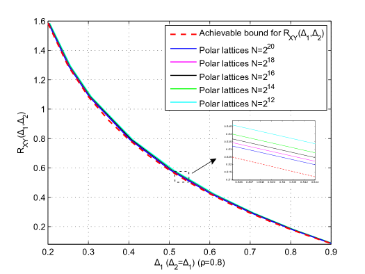
Fig. 8: Simulation performance for Gray-Wyner coding of two Gaussian sources in region $\varepsilon_{2}$. We set $\triangle_{1}=\triangle_{2}$, $\rho=0.8$. The blocklength of polar lattices of each level is given by $N=2^{12}$, $2^{14}$, $2^{16}$, $2^{18}$, $2^{20}$.

The region $\varepsilon_{3}$ is a degenerated region. If $\frac{\delta_{2}}{\delta_{1}}<\rho^{2}$, $R_{XY}\left(\triangle_{1},\triangle_{2}\right)=\frac{1}{2}\log\frac{1}{\triangle_{1}}$, which coincides with the rate-distortion function of a scalar Gaussian source. This means that the optimal coding strategy is to ignore $Y$ and simply compress $X$. Then $Y^{\prime}$ can be optimally estimated from $X^{\prime}$ by $Y^{\prime}=\rho X^{\prime}$. The case where $\frac{\delta_{1}}{\delta_{2}}<\rho^{2}$ can be solved similarly. Therefore the construction of polar lattices for a scalar Gaussian source given in [18] can be applied directly for this region.

VI Conclusion

Explicit construction of polar codes and polar lattices for both lossy and lossless Gray-Wyner coding is proposed. For discrete sources, the construction of polar codes is utilized to achieve the entire best-known region of lossless Gray-Wyner coding. The test channels for each part of the region are identified so that the operational meaning of the Wyner’s common information can be well interpreted. Moreover, polar codes are utilized to extract the common information of DSBS in the lossy Gray-Wyner problem. The constructions of polar codes to achieve the common information for each distortion region are presented, together with the simulation result. Additionally, an operational interpretation of the connection between the lossless and lossy Gray-Wyner coding are given in this work. With regard to Gaussian sources, the construction of polar lattices are shown to be able to extract the common information for each best-known distortion region. More importantly, it is found that the construction of a polar lattice for extracting the common information of a pair of Gaussian sources is equivalent to that for a single Gaussian source. This Gaussian source can be derived simply by a linear combination of the two original sources. Therefore, a rate-distortion bound achieving polar lattice designed for a Gaussian source can be directly used to extract the common information of a pair of Gaussian sources or even multiple Gaussian sources.

Appendix A Proof of Lemma 9

For $L$ joint Gaussian RVs $\mathbf{X}_{L}=\{X_{1},X_{2},\ldots X_{L}\}$ with covariance matrix $K_{L}$ as given in (14). The determinant of the covariance matrix is

$$\left|K_{L}\right|=\left(1+(L-1)\rho\right)\left(1-\rho\right)^{L-1},$$

and the inverse of $K_{L}$ is

$$K_{L}^{-1}=\frac{1}{-(L-1)\rho^{2}+(L-2)\rho+1}\begin{bmatrix}(L-2)\rho+1&-\rho&\cdots&-\rho\\ -\rho&(L-2)\rho+1&\cdots&-\rho\\ \vdots&\vdots&\ddots&\vdots\\ -\rho&-\rho&\cdots&(L-2)\rho+1\end{bmatrix}.$$

Therefore the joint distribution of $L$ Gaussian sources with covariance matrix $K_{L}$ follows the next expression:

$$\begin{aligned} &f_{\mathbf{X}_{L}}(\mathbf{x}_{L})\\ &=\frac{1}{\sqrt{(2\pi)^{L}\left|K_{L}\right|}}\exp\left(-\frac{1}{2}\mathbf{x}_{L}^{\mathrm{T}}K_{L}^{-1}\mathbf{x}_{L}\right)\\ &=\frac{1}{\sqrt{(2\pi)^{L}\left(1+(L-1)\rho\right)\left(1-\rho\right)^{L-1}}}\\ &\hskip 10.00002pt\cdot\exp\left[-\frac{1}{2\left(-(L-1)\rho^{2}+(L-2)\rho+1\right)}\left(\left(\left(L-2\right)\rho+1\right)\sum_{i=1}^{L}x_{i}^{2}-2\rho\sum_{\begin{aligned} i,j=1;i<j\end{aligned}}^{L}x_{i}x_{j}\right)\right].\end{aligned}$$

Since the components of $\mathbf{X}_{L}$ are conditionally independent given $W$, we have

$$f_{\mathbf{\bar{X}}_{L}}(\mathbf{x}_{L})$$ (17)

$$=\sum_{a\in\Lambda}f_{\bar{X}_{1},\bar{X}_{2},\ldots\bar{X}_{L},\bar{W}}\left(x_{1},x_{2},\ldots x_{L},a\right)$$

$$=\sum_{a\in\Lambda}f_{\bar{W}}(a)f_{\bar{X}_{1}|\bar{W}}(x_{1}|a)f_{\bar{X}_{2}|\bar{W}}(x_{2}|a)\ldots f_{\bar{X}_{L}|\bar{W}}(x_{L}|a)$$

$$=\frac{1}{f_{\sqrt{\rho}}\left(\Lambda\right)}\sum_{a\in\Lambda}\frac{1}{\sqrt{2\pi\rho}}\exp\left(-\frac{a^{2}}{2\rho}\right)\frac{1}{\sqrt{2\pi(1-\rho)}}\exp\left(-\frac{(x_{1}-a)^{2}}{2(1-\rho)}\right)\cdots\frac{1}{\sqrt{2\pi(1-\rho)}}\exp\left(-\frac{(x_{L}-a)^{2}}{2(1-\rho)}\right)$$

$$=\frac{1}{\sqrt{(2\pi)^{L}\left(1+(L-1)\rho\right)\left(1-\rho\right)^{L-1}}}$$

$$\hskip 20.00003pt\cdot\exp\left[-\frac{1}{2\left(-(L-1)\rho^{2}+(L-2)\rho+1\right)}\left(\left(\left(L-2\right)\rho+1\right)\sum_{i=1}^{L}x_{i}^{2}-2\rho\sum_{\begin{aligned} i,j=1;i<j\end{aligned}}^{L}x_{i}x_{j}\right)\right]$$

$$\hskip 20.00003pt\cdot\frac{1}{f_{\sqrt{\rho}}\left(\Lambda\right)}\sum_{a\in\Lambda}\frac{1}{\sqrt{\frac{2\pi\rho(1-\rho)}{1+(L-1)\rho}}}\exp\left[-\frac{1}{\frac{2\rho(1-\rho)}{1+(L-1)\rho}}\left(a-\frac{\rho}{1+(L-1)\rho}\left(x_{1}+\cdots+x_{L}\right)\right)^{2}\right]$$

$$=\frac{f_{\mathbf{X}_{L}}(\mathbf{x}_{L})}{f_{\sqrt{\rho}}\left(\Lambda\right)}\cdot\sum_{a\in\Lambda}\frac{1}{\sqrt{\frac{2\pi\rho(1-\rho)}{1+(L-1)\rho}}}\exp\left[-\frac{1}{\frac{2\rho(1-\rho)}{1+(L-1)\rho}}\left(a-\frac{\rho}{1+(L-1)\rho}\left(x_{1}+\cdots+x_{L}\right)\right)^{2}\right].$$

By the definition of the flatness factor (7), we have

$$\left|V(\Lambda)\sum_{a\in\Lambda}\frac{1}{\sqrt{\frac{2\pi\rho(1-\rho)}{1+(L-1)\rho}}}\exp\left[-\frac{1}{\frac{2\rho(1-\rho)}{1+(L-1)\rho}}\left(a-\frac{\rho\left(x_{1}+\cdots+x_{L}\right)}{1+(L-1)\rho}\right)^{2}\right]-1\right|$$ (18)

$$\leq\epsilon_{\Lambda}\left(\sqrt{\frac{\rho(1-\rho)}{1+(L-1)\rho}}\right)=\epsilon.$$

In this way, we derive a similar relation to (11). Moreover, we have $\epsilon\left(\sqrt{\rho}\right)\leq\epsilon$ since $\epsilon_{\Lambda}\left(\sigma\right)$ is monotonically decreasing of $\sigma$. Hence

$$\left|V(\Lambda)f_{\sqrt{\rho}}(\Lambda)-1\right|\leq\epsilon\left(\sqrt{\rho}\right)\leq\epsilon.$$ (19)

Combining $\left(\ref{eq:Gaussian joint L sources}\right)$, $\left(\ref{eq:FlatnessFactorL}\right)$ and $\left(\ref{eq:FlatnessFactorL2}\right)$ gives us

$$f_{\mathbf{X}_{L}}(\mathbf{x}_{L})\left(1-2\epsilon\right)\leq f_{\mathbf{X}_{L}}(\mathbf{x}_{L})\frac{1-\epsilon}{1+\epsilon}\leq f_{\mathbf{\bar{X}}_{L}}(\mathbf{x}_{L}),$$

and

$$f_{\mathbf{\bar{X}}_{L}}(\mathbf{x}_{L})\leq f_{\mathbf{X}_{L}}(\mathbf{x}_{L})\frac{1+\epsilon}{1-\epsilon}\leq f_{\mathbf{X}_{L}}(\mathbf{x}_{L})\left(1+4\epsilon\right),$$

when $\epsilon<\frac{1}{2}$. Finally,

$$\int_{\mathbb{R}^{L}}\left|f_{\mathbf{\bar{X}}_{L}}(\mathbf{x}_{L})-f_{\mathbf{X}_{L}}(\mathbf{x}_{L})\right|dx_{1}dx_{2}\ldots dx_{L}\leq 4\epsilon\int_{\mathbb{R}^{L}}f_{\mathbf{X}_{L}}(\mathbf{x}_{L})dx_{1}dx_{2}\ldots dx_{L}=4\epsilon.$$

Similarly, the Kullback-Leibler divergence between $f_{\mathbf{\bar{X}}_{L}}(\mathbf{x}_{L})$ and $f_{\mathbf{X}_{L}}(\mathbf{x}_{L})$ can be upper-bounded as

$$\mathbb{D}\left(f_{\mathbf{\bar{X}}_{L}}(\mathbf{x}_{L})\|f_{\mathbf{X}_{L}}(\mathbf{x}_{L})\right) =\int_{\mathbb{R}^{L}}f_{\mathbf{\bar{X}}_{L}}(\mathbf{x}_{L})\log\frac{f_{\mathbf{\bar{X}}_{L}}(\mathbf{x}_{L})}{f_{\mathbf{X}_{L}}(\mathbf{x}_{L})}dx_{1}dx_{2}\ldots dx_{L}$$ (20)

$$\leq\int_{\mathbb{R}^{L}}f_{\mathbf{\bar{X}}_{L}}(\mathbf{x}_{L})\log(1+4\epsilon)dx_{1}dx_{2}\ldots dx_{L}$$

$$=\log(1+4\epsilon).$$

For any $\sqrt{\frac{\rho(1-\rho)}{1+(L-1)\rho}}>0$, $\epsilon$ can be made arbitrarily small by scaling $\Lambda$. Therefore, $\bar{W}$ can be viewed as the common message when $\epsilon\rightarrow 0$, according to Wyner’s second approach. To show that $I\left(\mathbf{\bar{X}}_{L};\bar{W}\right)$ can be arbitrarily close to the common information, we rewrite $\mathbb{D}\left(f_{\mathbf{\bar{X}}_{L}}(\mathbf{x}_{L})\|f_{\mathbf{X}_{L}}(\mathbf{x}_{L})\right)$ as

$$\mathbb{D}\left(f_{\mathbf{\bar{X}}_{L}}(\mathbf{x}_{L})\|f_{\mathbf{X}_{L}}(\mathbf{x}_{L})\right)$$

$$=\int_{\mathbb{R}^{L}}f_{\mathbf{\bar{X}}_{L}}(\mathbf{x}_{L})\log\frac{f_{\mathbf{\bar{X}}_{L}}(\mathbf{x}_{L})}{f_{\mathbf{X}_{L}}(\mathbf{x}_{L})}dx_{1}dx_{2}\ldots dx_{L}$$

$$=-\int_{\mathbb{R}^{L}}f_{\mathbf{\bar{X}}_{L}}(\mathbf{x}_{L})\log f_{\mathbf{X}_{L}}(\mathbf{x}_{L})dx_{1}dx_{2}\ldots dx_{L}-h(\mathbf{\bar{X}}_{L})$$

$$=-\int_{\mathbb{R}^{L}}f_{\mathbf{\bar{X}}_{L}}(\mathbf{x}_{L})\log\left[\frac{1}{\sqrt{(2\pi)^{L}\left(1+(L-1)\rho\right)\left(1-\rho\right)^{L-1}}}\right.$$

$$\hskip 10.00002pt\cdot\left.\exp\left[-\frac{1}{2\left(-(L-1)\rho^{2}+(L-2)\rho+1\right)}\left(\left(\left(L-2\right)\rho+1\right)\sum_{i=1}^{L}x_{i}^{2}-2\rho\sum_{\begin{aligned} i,j=1;i<j\end{aligned}}^{L}x_{i}x_{j}\right)\right]\right]dx_{1}\ldots dx_{L}-h(\mathbf{\bar{X}}_{L})$$

$$=\log\left(\sqrt{(2\pi)^{L}\left(1+(L-1)\rho\right)\left(1-\rho\right)^{L-1}}\right)-h(\mathbf{\bar{X}}_{L})$$

$$\hskip 10.00002pt+\mathsf{E_{\mathbf{\bar{X}}_{L}}}\left[\left(\left(L-2\right)\rho+1\right)\sum_{i=1}^{L}x_{i}^{2}-2\rho\sum_{\begin{aligned} i,j=1;i<j\end{aligned}}^{L}x_{i}x_{j}\right]\frac{\log\left(e\right)}{2\left(-(L-1)\rho^{2}+(L-2)\rho+1\right)}$$

$$=\log\left(\sqrt{(2\pi)^{L}\left(1+(L-1)\rho\right)\left(1-\rho\right)^{L-1}}\right)-h(\mathbf{\bar{X}}_{L})+\frac{L}{2}\frac{\mathsf{E_{\bar{W}}}\left[w^{2}\right]+(L-2)\rho+1}{(L-1)\rho+1}\log\left(e\right).$$

Notice that $\mathsf{E}_{\bar{W}}\left[w^{2}\right]\geq\rho(1-2\epsilon)$ by [28, Lemma 5] and [28, Remark 3]. Hence

$$\mathbb{D}\left(f_{\mathbf{\bar{X}}_{L}}(\mathbf{x}_{L})\|f_{\mathbf{X}_{L}}(\mathbf{x}_{L})\right)$$

$$\geq\log\left(\sqrt{(2\pi)^{L}\left(1+(L-1)\rho\right)\left(1-\rho\right)^{L-1}}\right)-h(\mathbf{\bar{X}}_{L})+\left(\frac{L}{2}-\frac{L\rho}{(L-1)\rho+1}\epsilon\right)\log\left(e\right)$$

$$\geq\log\left(\sqrt{(2\pi)^{L}\left(1+(L-1)\rho\right)\left(1-\rho\right)^{L-1}}\right)-h(\mathbf{\bar{X}}_{L})+\left(\frac{L}{2}-\epsilon\right)\log\left(e\right)$$

$$=h(\mathbf{X}_{L})-h(\mathbf{\bar{X}}_{L})-\epsilon\log\left(e\right).$$

Using $\left(\ref{eq:LGaussianKLdistance}\right)$, we obtain

$$I\left(\mathbf{X}_{L};W\right)-I\left(\mathbf{\bar{X}}_{L};\bar{W}\right) =h(\mathbf{X}_{L})-h(\mathbf{\bar{X}}_{L})$$

$$\leq\log(1+4\epsilon)+\epsilon\log\left(e\right)$$

$$\leq 5\epsilon\log\left(e\right).$$

Appendix B Proof of Theorem 10

Let $\bar{W}$ be labeled by bits $\bar{W}_{1}^{r}=\{\bar{W}_{1},\ldots,\bar{W}_{r}\}$ according to a binary partition chain $\Lambda/\Lambda_{1}/\cdots/\Lambda_{r-1}/\Lambda^{\prime}$ ($\Lambda^{\prime}$ also refers to $\Lambda_{r}$). $D_{\Lambda,\sqrt{\rho}}$ induces a distribution $P_{\bar{W}_{1}^{r}}$ whose limit corresponds to $D_{\Lambda,\sqrt{\rho}}$ as $r\rightarrow\infty$.

By the chain rule of mutual information

$$I(\mathbf{\bar{X}}_{L};\bar{W}_{1}^{r})=\sum_{l=1}^{r}I(\mathbf{\bar{X}}_{L};\bar{W}_{l}|\bar{W}_{1}^{l-1}),$$

we obtain $r$ binary-input test channels $V_{l}$ for $1\leq l\leq r$. Given the realization $w_{1}^{l}$ of $\bar{W}_{1}^{r}$, denote by $\mathcal{A}_{\ell}(w_{1}^{\ell})$ the coset of $\Lambda_{l}$ indexed by $w_{1}^{l-1}$ and $w_{l}$. According to [30], the channel transition PDF of the $l$-th channel $V_{l}$ is given by

$$f_{\mathbf{\bar{X}}_{L}|\bar{W}_{l},\bar{W}_{1}^{l-1}}\left(\mathbf{x}_{L}|w_{l},w_{1}^{l-1}\right)$$

$$=\frac{1}{f_{\sqrt{\rho}}(\mathcal{A}_{\ell}(w_{1}^{\ell}))}\sum_{a\in\mathcal{A}_{\ell}(w_{1}^{\ell})}f_{\sqrt{\rho}}(a)f_{\mathbf{\bar{X}}_{L}|\bar{W}}(\mathbf{x}_{L}|a)$$

$$=\frac{1}{f_{\sqrt{\rho}}(\mathcal{A}_{\ell}(w_{1}^{\ell}))}\sum_{a\in\mathcal{A}_{\ell}(w_{1}^{\ell})}\frac{1}{\sqrt{2\pi\rho}}\exp\bigg{(}-\frac{a^{2}}{2\rho}\bigg{)}\frac{1}{\sqrt{2\pi(1-\rho)}}\exp\bigg{(}-\frac{(x_{1}-a)^{2}}{2(1-\rho)}\bigg{)}\cdots\frac{1}{\sqrt{2\pi(1-\rho)}}\exp\bigg{(}-\frac{(x_{L}-a)^{2}}{2(1-\rho)}\bigg{)}$$

$$=\frac{1}{\sqrt{(2\pi)^{L}\left(1+(L-1)\rho\right)\left(1-\rho\right)^{L-1}}}$$

$$\hskip 10.00002pt\cdot\exp\left[-\frac{1}{2\left(-(L-1)\rho^{2}+(L-2)\rho+1\right)}\left(\left(\left(L-2\right)\rho+1\right)\sum_{i=1}^{L}x_{i}^{2}-2\rho\sum_{\begin{aligned} i,j=1;i<j\end{aligned}}^{L}x_{i}x_{j}\right)\right]$$

$$\hskip 10.00002pt\cdot\frac{1}{f_{\sqrt{\rho}}(\mathcal{A}_{\ell}(w_{1}^{\ell}))}\sum_{a\in\mathcal{A}_{\ell}(w_{1}^{\ell})}\frac{1}{\sqrt{\frac{2\pi\rho(1-\rho)}{1+(L-1)\rho}}}\exp\left[-\frac{1}{\frac{2\rho(1-\rho)}{1+(L-1)\rho}}\left(a-\frac{\rho}{1+(L-1)\rho}\left(x_{1}+\cdots+x_{L}\right)\right)^{2}\right],$$

Let $\tilde{V}_{l}$ be a symmetrized channel with input $\tilde{W}_{l}$ (assume to be uniformly distributed) and output $\left(\mathbf{\bar{X}}_{L},\bar{W}_{1}^{\ell-1},\bar{W}_{l}\oplus\tilde{W}_{l}\right)$, built from the asymmetric channel $V_{l}$. Then the joint PDF of $V_{l}$ can be represented by the transition PDF of $\tilde{V}_{l}$ (see [22] for more details), as shown in the following equation.

$$f_{\tilde{V}_{\ell}}(\mathbf{x}_{L},w_{1}^{\ell-1},w_{\ell}\oplus\tilde{w}_{\ell}|\tilde{w}_{\ell})$$ (21)

$$=f_{\mathbf{\bar{X}}_{L},\bar{W}_{1}^{\ell}}(\mathbf{x}_{L},w_{1}^{\ell})$$

$$=\frac{1}{\sqrt{(2\pi)^{L}\left(1+(L-1)\rho\right)\left(1-\rho\right)^{L-1}}}$$

$$\hskip 10.00002pt\cdot\exp\left[-\frac{1}{2\left(-(L-1)\rho^{2}+(L-2)\rho+1\right)}\left(\left(\left(L-2\right)\rho+1\right)\sum_{i=1}^{L}x_{i}^{2}-2\rho\sum_{\begin{aligned} i,j=1;i<j\end{aligned}}^{L}x_{i}x_{j}\right)\right]$$

$$\hskip 10.00002pt\cdot\frac{1}{f_{\sqrt{\rho}}(\Lambda)}\sum_{a\in\mathcal{A}_{\ell}(w_{1}^{\ell})}\frac{1}{\sqrt{\frac{2\pi\rho(1-\rho)}{1+(L-1)\rho}}}\exp\left[-\frac{1}{\frac{2\rho(1-\rho)}{1+(L-1)\rho}}\left(a-\frac{L\rho}{1+(L-1)\rho}\frac{\left(x_{1}+\cdots+x_{L}\right)}{L}\right)^{2}\right].$$

Comparing with the $\Lambda_{\ell-1}/\Lambda_{\ell}$ channel [22, Equation (13)], we see that the symmetrized channel (13) is equivalent to a $\Lambda_{\ell-1}/\Lambda_{\ell}$ channel with noise variance $\frac{\rho(1-\rho)}{1+(L-1)\rho}$ in the sense of the likelihood ratio.

$\mathbf{X}_{L}=\{X_{1},X_{2},\ldots X_{L}\}$ are Gaussian RVs with zero mean and covariance matrix $K_{L}$ as given in (14). The mean value and variance of the Gaussian RV $\frac{X_{1}+\cdots+X_{L}}{L}$ are respectively

$$\mathsf{E}\left[\frac{X_{1}+\cdots+X_{L}}{L}\right]=\frac{1}{L}\left(\mathsf{E}\left[X_{1}\right]+\ldots+\mathsf{E}\left[X_{L}\right]\right)=0,$$

and

$$\sigma^{2}\left(\frac{X_{1}+\cdots+X_{L}}{L}\right) \mathsf{=E}\left[\left(\frac{X_{1}+\cdots+X_{L}}{L}\right)^{2}\right]-\left(\mathsf{E}\left[\frac{X_{1}+\cdots+X_{L}}{L}\right]\right)^{2}$$

$$=\frac{1}{L^{2}}\left(\mathsf{E}\left[\sum_{i=1}^{L}X_{i}^{2}+2\rho\sum_{\begin{aligned} i,j=1;i<j\end{aligned}}^{L}X_{i}X_{j}\right]\right)$$

$$=\frac{L+2\rho\begin{pmatrix}L\\ 2\end{pmatrix}}{L^{2}}=\frac{1+\left(L-1\right)\rho}{L},$$

where $\begin{pmatrix}L\\ r\end{pmatrix}\triangleq\frac{L!}{r!\left(L-r\right)!}$.

Consider the construction of a polar lattice to quantize $\frac{X_{1}+X_{2}+\ldots+X_{L}}{L}$ using reconstruction distribution $D_{\Lambda,\sqrt{\rho}}$. Denote the variance of the source and the reconstruction by $\sigma_{s}^{2}=\frac{1+\left(L-1\right)\rho}{L}$ and $\sigma_{r}^{2}=\rho$, respectively. Thus, the variance of the noise equals $\sigma_{z}^{2}=\sigma_{s}^{2}-\sigma_{r}^{2}=\frac{1-\rho}{L}$. Then we apply MMSE to this relation. By definitions, the MMSE scaling coefficient $\alpha$ and noise variance $\tilde{\sigma}_{z}^{2}$ are given by

$$\alpha=\frac{\sigma_{r}^{2}}{\sigma_{s}^{2}}=\frac{L\rho}{1+\left(L-1\right)\rho},$$

$$\tilde{\sigma}_{z}^{2}=\alpha\cdot\sigma_{z}^{2}=\frac{\rho(1-\rho)}{1+\left(L-1\right)\rho},$$

which are the same to those in the summation section of $\left(\ref{eq:AppTheoremSymm}\right)$.

Appendix C Proof of Lemma 11

The PDF of $\left(X,Y\right)$ can be represented from the PDF of $\left(\bar{X},\bar{Y}\right)$ as follows.

$$f_{\bar{X},\bar{Y}}\left(x,y\right)$$ (22)

$$=\sum_{a\in\varLambda}f_{\bar{X^{\prime}}}(a)f_{\bar{X},\bar{Y}|\bar{X^{\prime}}}\left(x,y|a\right)$$

$$=\sum_{a\in\varLambda}f_{\bar{X^{\prime}}}(a)f_{Z_{1}Z_{2}}\left(x-a,y-\sqrt{\frac{\delta_{2}}{\delta_{1}}}a\right)$$

$$=\frac{1}{f_{\sqrt{\delta_{1}}}\left(\Lambda\right)}\sum_{a\in\Lambda}\frac{1}{\sqrt{2\pi\delta_{1}}}\exp\left(-\frac{a^{2}}{2\delta_{1}}\right)\frac{1}{2\pi\sqrt{\triangle_{1}\triangle_{2}-\left(\rho-\sqrt{\delta_{1}\delta_{2}}\right)^{2}}}$$

$$\hskip 10.00002pt\cdot\exp\left[-\frac{1}{2\left(1-\frac{\left(\rho-\sqrt{\delta_{1}\delta_{2}}\right)^{2}}{\triangle_{1}\triangle_{2}}\right)}\left(\frac{\left(x-a\right)^{2}}{\triangle_{1}}+\frac{\left(y-\sqrt{\frac{\delta_{2}}{\delta_{1}}}a\right)^{2}}{\triangle_{2}}-\frac{2\left(\rho-\sqrt{\delta_{1}\delta_{2}}\right)\left(x-a\right)\left(y-\sqrt{\frac{\delta_{2}}{\delta_{1}}}a\right)}{\triangle_{1}\triangle_{2}}\right)\right]$$

$$=\frac{1}{2\pi\sqrt{1-\rho^{2}}}\exp\left[-\frac{\left(x^{2}+y^{2}-2\rho xy\right)}{2\left(1-\rho^{2}\right)}\right]\frac{1}{f_{\sqrt{\delta_{1}}}\left(\Lambda\right)}\sum_{a\in\Lambda}\sqrt{\frac{1-\rho^{2}}{2\pi\delta_{1}\left(\triangle_{1}\triangle_{2}-\left(\rho-\sqrt{\delta_{1}\delta_{2}}\right)^{2}\right)}}$$

$$\hskip 10.00002pt\cdot\exp\left[-\frac{1-\rho^{2}}{2\delta_{1}\left(\triangle_{1}\triangle_{2}-\left(\rho-\sqrt{\delta_{1}\delta_{2}}\right)^{2}\right)}\left(a-\frac{\left(\delta_{1}-\rho\sqrt{\delta_{1}\delta_{2}}\right)x+\left(\sqrt{\delta_{1}\delta_{2}}-\delta_{1}\rho\right)y}{1-\rho^{2}}\right)^{2}\right],$$

where $\frac{1}{2\pi\sqrt{1-\rho^{2}}}\exp\bigg{(}-\frac{x^{2}+y^{2}-2\rho xy}{2(1-\rho^{2})}\bigg{)}=f_{X,Y}(x,y)$ is the PDF of two joint Gaussian RVs. By the definition of the flatness factor (7), we have

$$\left|V\left(\Lambda\right)\sum_{a\in\Lambda}\sqrt{\frac{1-\rho^{2}}{2\pi\delta_{1}\left(\triangle_{1}\triangle_{2}-\left(\rho-\sqrt{\delta_{1}\delta_{2}}\right)^{2}\right)}}\right.$$ (23)

$$\left.\hskip 10.00002pt\cdot\exp\left[-\frac{1-\rho^{2}}{2\delta_{1}\left(\triangle_{1}\triangle_{2}-\left(\rho-\sqrt{\delta_{1}\delta_{2}}\right)^{2}\right)}\left(a-\frac{\left(\delta_{1}-\rho\sqrt{\delta_{1}\delta_{2}}\right)x+\left(\sqrt{\delta_{1}\delta_{2}}-\delta_{1}\rho\right)y}{1-\rho^{2}}\right)^{2}\right]-1\right|$$

$$\leq\epsilon_{\Lambda}\left(\sqrt{\frac{\delta_{1}\left(\triangle_{1}\triangle_{2}-\left(\rho-\sqrt{\delta_{1}\delta_{2}}\right)^{2}\right)}{1-\rho^{2}}}\right)=\epsilon.$$

Since $\epsilon_{\Lambda}\left(\sigma\right)$ is a monotonically decreasing function of $\sigma$ and the fact that

$$\triangle_{1}\triangle_{2}-\left(\rho-\sqrt{\delta_{1}\delta_{2}}\right)^{2}-1+\rho^{2}$$

$$=2\rho\sqrt{\delta_{1}\delta_{2}}-\delta_{1}-\delta_{2}$$

$$=-\left(\sqrt{\delta_{1}}-\sqrt{\delta_{2}}\right)^{2}-2\sqrt{\delta_{1}\delta_{2}}\left(1-\rho\right)\leq 0,$$

we have

$$\frac{\triangle_{1}\triangle_{2}-\left(\rho-\sqrt{\delta_{1}\delta_{2}}\right)^{2}}{1-\rho^{2}} \leq 1.$$

Therefore, it implies $\epsilon\left(\sqrt{\delta_{1}}\right)\leq\epsilon$ and more specifically

$$\left|V\left(\Lambda\right)f_{\sqrt{\delta_{1}}}\left(\Lambda\right)-1\right|\leq\epsilon.$$ (24)

From the above results (22), (23) and (24), we have

$$f_{X,Y}\left(x,y\right)\left(1-2\epsilon\right)\leq f_{X,Y}\left(x,y\right)\frac{1-\epsilon}{1+\epsilon}\leq f_{\bar{X},\bar{Y}}\left(x,y\right),$$

and

$$f_{\bar{X},\bar{Y}}\left(x,y\right)\leq f_{X,Y}\left(x,y\right)\frac{1+\epsilon}{1-\epsilon}\leq f_{X,Y}\left(x,y\right)\left(1-4\epsilon\right),$$

when $\epsilon<0.5$. Finally,

$$\int_{\mathbb{R}^{2}}\left|f_{\bar{X},\bar{Y}}(x,y)-f_{X,Y}(x,y)\right|dxdy$$

$$\leq 4\epsilon\int_{\mathbb{R}^{2}}f_{X,Y}(x,y)dxdy=4\epsilon.$$

Similarly, the Kullback-Leibler divergence between $f_{\bar{X},\bar{Y}}(x,y)$ and $f_{X,Y}(x,y)$ can be upper-bounded as

$$\mathbb{D}(f_{\bar{X},\bar{Y}}\|f_{X,Y}) =\int_{\mathbb{R}^{2}}f_{\bar{X},\bar{Y}}(x,y)\log\frac{f_{\bar{X},\bar{Y}}(x,y)}{f_{X,Y}(x,y)}dxdy$$ (25)

$$\leq\int_{\mathbb{R}^{2}}f_{\bar{X},\bar{Y}}(x,y)\log(1+4\epsilon)dxdy$$

$$=\log(1+4\epsilon).$$

For any $\sqrt{\frac{\delta_{1}\left(\triangle_{1}\triangle_{2}-\left(\rho-\sqrt{\delta_{1}\delta_{2}}\right)^{2}\right)}{1-\rho^{2}}}>0$, $\epsilon$ can be made arbitrarily small by scaling $\Lambda$. To show that $I\left(\bar{X},\bar{Y};\bar{X^{\prime}}\right)$ can be arbitrarily close to $I\left(X,Y;X^{\prime}\right)$, we rewrite $\mathbb{D}(f_{\bar{X},\bar{Y}}\|f_{X,Y})$ as

$$\mathbb{D}(f_{\bar{X},\bar{Y}}\|f_{X,Y})$$

$$=\int_{\mathbb{R}^{2}}f_{\bar{X},\bar{Y}}(x,y)\log\frac{f_{\bar{X},\bar{Y}}(x,y)}{f_{X,Y}(x,y)}dxdy$$

$$=-\int_{\mathbb{R}^{2}}f_{\bar{X},\bar{Y}}(x,y)\log f_{X,Y}(x,y)dxdy-h(\bar{X},\bar{Y})$$

$$=-\int_{\mathbb{R}^{2}}f_{\bar{X},\bar{Y}}(x,y)\log\left(\frac{1}{2\pi\sqrt{1-\rho^{2}}}\exp\bigg{(}-\frac{x^{2}+y^{2}-2\rho xy}{2(1-\rho^{2})}\bigg{)}\right)dxdy-h(\bar{X},\bar{Y})$$

$$=\log\big{(}2\pi\sqrt{1-\rho^{2}}\big{)}+\frac{\mathsf{E}_{\bar{X},\bar{Y}}[x^{2}+y^{2}-2\rho xy]}{2(1-\rho^{2})}\log(e)-h(\bar{X},\bar{Y})$$

$$=\log\big{(}2\pi\sqrt{1-\rho^{2}}\big{)}+\log(e)-h(\bar{X},\bar{Y}),$$

based on the fact that $\mathsf{E}_{\bar{X},\bar{Y}}\left[x,y\right]=\rho$ and $\mathsf{E}_{\bar{X},\bar{Y}}\left[x^{2}\right]=\mathsf{E}_{\bar{X},\bar{Y}}\left[y^{2}\right]=1$. Trivially we have

$$\mathbb{D}(f_{\bar{X},\bar{Y}}\|f_{X,Y}) \geq\log\big{(}2\pi\sqrt{1-\rho^{2}}\big{)}+(1-\epsilon)\log(e)-h(\bar{X},\bar{Y})$$

$$=h(X,Y)-h(\bar{X},\bar{Y})-\epsilon\log(e).$$

Using (25), we obtain

$$I(X,Y;X^{\prime})-I(\bar{X},\bar{Y};\bar{X^{\prime}}) =h(X,Y)-h(\bar{X},\bar{Y})$$

$$\leq\log(1+4\epsilon)+\epsilon\log(e)$$

$$\leq 5\epsilon\log(e).$$

Appendix D Proof of Theorem 12

Since this proof uses multilevel coding, the notations are changed differently from the rest of the paper.

Notations: Denote $X_{l}$ a RV $X$ at level $l$. The $i$-th realization of $X_{l}$ is denoted by $x_{l}^{i}$. The notation $x_{l}^{i:j}$ denotes vector $\left(x_{l}^{i},\ldots x_{l}^{j}\right)$, which is a realization of RVs $X_{l}^{i:j}=\left(X_{l}^{i},\ldots X_{l}^{j}\right)$. Similarly, $x_{l:j}^{i}$ denotes the realization of the $i$-th RV from level $l$ to level $j$. $X_{l}^{\mathcal{I}}$ denotes the subvector $\left\{X_{l}^{i}\right\}_{i\in\mathcal{I}}$ at level $l$. For the consistency of notations in this proof, let $X^{1:N}$ denote a vector $\left(X^{1},\ldots,X^{N}\right)$ and $x^{i}$ denote the $i$-th realization of RV $X^{i}$.

Firstly, for the sources $\left(\bar{X},\bar{Y}\right)$ and reconstruction RVs $\left(\bar{X^{\prime}},\bar{Y^{\prime}}\right)$, we consider the average performance of the multilevel polar codes with all possible choice of frozen sets $u_{l}^{\mathcal{F}_{l}}$ (defined in [18, Equation (16)]) at each level. If the encoding rule described in the form of [18, Equation (17)] is used for all $i\in[N]$ at each level, the resulted average distortions of $\left(\bar{X},\bar{Y}\right)$ are given by

$$\triangle_{P,\bar{X}} =\frac{1}{N}\sum_{u_{1:r}^{1:N},\bar{x}^{1:N}}P_{U_{1:r}^{1:N},\bar{X}^{1:N}}\left(u_{1:r}^{1:N},\bar{x}^{1:N}\right)d\left(\bar{x}^{1:N},\mathcal{M}\left(u_{1:r}^{1:N}G_{N}\right)\right),$$

$$\triangle_{P,\bar{Y}} =\frac{1}{N}\sum_{u_{1:r}^{1:N},\bar{y}^{1:N}}P_{U_{1:r}^{1:N},\bar{Y}^{1:N}}\left(u_{1:r}^{1:N},\bar{y}^{1:N}\right)d\left(\bar{y}^{1:N},\mathcal{M}\left(\sqrt{\frac{\delta_{2}}{\delta_{1}}}u_{1:r}^{1:N}G_{N}\right)\right),$$

where $\mathcal{M}\left(u_{1:r}^{1:N}G_{N}\right)$ denotes a mapping from $u_{1:r}^{1:N}$ to $\bar{x^{\prime}}{}^{1:N}$ according to [18, Equation (38)]. Due to the linear relation $\bar{Y^{\prime}}=\sqrt{\frac{\delta_{2}}{\delta_{1}}}\bar{X^{\prime}}$ for region $\varepsilon_{2}$, we have $\bar{x^{\prime}}{}_{l}^{1:N}=u_{l}^{1:N}G_{N}$ and $\bar{y^{\prime}}{}_{l}^{1:N}=\sqrt{\frac{\delta_{2}}{\delta_{1}}}u_{l}^{1:N}G_{N}$ for each level. When $r\rightarrow\infty$, there exist an one-to-one mapping from $u_{1:r}^{1:N}$ to $\bar{x^{\prime}}{}^{1:N}$ and $\bar{y^{\prime}}{}^{1:N}$. Thus, we have

$$\triangle_{P,\bar{X}}$$

$$=\frac{1}{N}\sum_{\bar{x^{\prime}}^{1:N},\bar{x}^{1:N}}P_{\bar{X^{\prime}}^{1:N},\bar{X}^{1:N}}\left(\bar{x^{\prime}}^{1:N},\bar{x}^{1:N}\right)d^{N}\left(\bar{x^{\prime}}^{1:N},\bar{x}^{1:N}\right)$$

$$=N\cdot\frac{1}{N}\sum_{\bar{x^{\prime}},\bar{x}}P_{\bar{X^{\prime}},\bar{X}}\left(\bar{x^{\prime}},\bar{x}\right)d\left(\bar{x^{\prime}},\bar{x}\right)$$

$$=\sum_{\bar{x^{\prime}}\in\Lambda}P_{\bar{X^{\prime}}}\left(\bar{x^{\prime}}\right)\int_{-\infty}^{+\infty}\frac{1}{\sqrt{2\pi\triangle_{1}}}\exp\left(-\frac{\left(\bar{x}-\bar{x^{\prime}}\right)^{2}}{2\triangle_{1}}\right)\left(\bar{x}-\bar{x^{\prime}}\right)^{2}d\bar{x}$$

$$=\triangle_{1}.$$

We can apply this distortion to source $\bar{Y}$ in a similar manner and derive $\triangle_{P,\bar{Y}}=\triangle_{2}$. The results $\triangle_{P,\bar{X}}=\triangle_{1}$ and $\triangle_{P,\bar{Y}}=\triangle_{2}$ are reasonable since the encoder does not do any compression. Next we replace $P_{U_{1:r}^{1:N},\bar{X}^{1:N}}\left(u_{1:r}^{1:N},\bar{x}^{1:N}\right)$ to $Q_{U_{1:r}^{1:N},\bar{X}^{1:N}}\left(u_{1:r}^{1:N},\bar{x}^{1:N}\right)$ and $P_{U_{1:r}^{1:N},\bar{Y}^{1:N}}\left(u_{1:r}^{1:N},\bar{y}^{1:N}\right)$ to $Q_{U_{1:r}^{1:N},\bar{Y}^{1:N}}\left(u_{1:r}^{1:N},\bar{y}^{1:N}\right)$, so that the encoder compresses $\left(\bar{X}^{1:N},\bar{Y}^{1:N}\right)$ to $U_{l}^{\mathcal{I}_{l}}$ at each level according to the rule [18, Equation (17)]. The result average distortion $\triangle_{Q,\bar{X}}$ can be bounded as

$$\triangle_{Q,\bar{X}}$$

$$=\frac{1}{N}\sum_{u_{1:r}^{1:N},\bar{x}^{1:N}}Q_{U_{1:r}^{1:N},\bar{X}^{1:N}}\left(u_{1:r}^{1:N},\bar{x}^{1:N}\right)d\left(\bar{x}^{1:N},\mathcal{M}\left(u_{1:r}^{1:N}G_{N}\right)\right)$$

$$\leq\frac{1}{N}\sum_{u_{1:r}^{1:N},\bar{x}^{1:N}}P_{U_{1:r}^{1:N},\bar{X}^{1:N}}\left(u_{1:r}^{1:N},\bar{x}^{1:N}\right)d\left(\bar{x}^{1:N},\mathcal{M}\left(u_{1:r}^{1:N}G_{N}\right)\right)$$

$$\hskip 10.00002pt+\frac{1}{N}\sum_{u_{1:r}^{1:N},\bar{x}^{1:N}}\left|P_{U_{1:r}^{1:N},\bar{X}^{1:N}}\left(u_{1:r}^{1:N},\bar{x}^{1:N}\right)-Q_{U_{1:r}^{1:N},\bar{X}^{1:N}}\left(u_{1:r}^{1:N},\bar{x}^{1:N}\right)\right|d\left(\bar{x}^{1:N},\mathcal{M}\left(u_{1:r}^{1:N}G_{N}\right)\right)$$

$$\leq\triangle_{P,\bar{X}}+\frac{1}{N}\cdot Nd_{\max x}2\mathbb{V}\left(P_{U_{1:r}^{1:N},\bar{X}^{1:N}}\left(u_{1:r}^{1:N},\bar{x}^{1:N}\right),Q_{U_{1:r}^{1:N},\bar{X}^{1:N}}\left(u_{1:r}^{1:N},\bar{x}^{1:N}\right)\right)$$

$$=\triangle_{1}+\mathcal{O}\left(2^{-N^{\beta^{\prime}}}\right),$$

where $d_{\max x}$ is assumed to be the maximum distortion between $\bar{x}$ and $\bar{x^{\prime}}$. The last equality follows from [18, Equation (20)] and $r=\mathcal{O}\left(\log\log N\right)$ [22, Lemma 5]. Similarly, we also have $\triangle_{Q,\bar{Y}}=\triangle_{2}+\mathcal{O}\left(2^{-N^{\beta^{\prime}}}\right)$ for source $\bar{Y}$.

Now we quantize the Gaussian sources $\left(X,Y\right)$ by the same encoder. Again we take the source $X$ as example. The resulted distortion $\triangle_{Q,X}$ can be written as

$$\triangle_{Q,X}$$

$$=\frac{1}{N}\sum_{u_{1:r}^{1:N},x^{1:N}}Q_{U_{1:r}^{1:N},X^{1:N}}\left(u_{1:r}^{1:N},x^{1:N}\right)d\left(x^{1:N},\mathcal{M}\left(u_{1:r}^{1:N}G_{N}\right)\right)$$

$$=\frac{1}{N}\sum_{u_{1:r}^{1:N},x^{1:N}}P_{X^{1:N}}\left(x^{1:N}\right)Q_{U_{1:r}^{1:N}\mid X^{1:N}}\left(u_{1:r}^{1:N}\mid x^{1:N}\right)d\left(x^{1:N},\mathcal{M}\left(u_{1:r}^{1:N}G_{N}\right)\right),$$

Since the same encoder is used, we apply the same realizations $\left(x^{1:N},y^{1:N}\right)$ for both RV pairs $\left(X^{1:N},Y^{1:N}\right)$ and $\left(\bar{X}^{1:N},\bar{Y}^{1:N}\right)$. Then the relation holds

$$Q_{U_{1:r}^{1:N}\mid X^{1:N}}\left(u_{1:r}^{1:N}\mid x^{1:N}\right) =Q_{U_{1:r}^{1:N}\mid\bar{X}^{1:N}}\left(u_{1:r}^{1:N}\mid x^{1:N}\right),$$

and hence

$$\triangle_{Q,X}-\triangle_{Q,\bar{X}}$$

$$=\frac{1}{N}\sum_{u_{1:r}^{1:N},x^{1:N}}\left(P_{X^{1:N}}\left(x^{1:N}\right)-P_{\bar{X}^{1:N}}\left(x^{1:N}\right)\right)$$

$$\hskip 20.00003pt\cdot Q_{U_{1:r}^{1:N}\mid X^{1:N}}\left(u_{1:r}^{1:N}\mid x^{1:N}\right)\cdot d\left(x^{1:N},\mathcal{M}\left(u_{1:r}^{1:N}G_{N}\right)\right)$$

$$\leq\frac{1}{N}\sum_{x^{1:N}}\left|P_{X^{1:N}}\left(x^{1:N}\right)-P_{\bar{X}^{1:N}}\left(x^{1:N}\right)\right|Nd_{\max x}.$$

By the telescoping expansion,

$$\sum_{x^{1:N}}\left|P_{X^{1:N}}\left(x^{1:N}\right)-P_{\bar{X}^{1:N}}\left(x^{1:N}\right)\right|$$

$$=\sum_{x^{1:N}}\sum_{i=1}^{N}\left|P_{X^{i}}\left(x^{i}\right)-P_{\bar{X}^{i}}\left(x^{i}\right)\right|P_{X^{1:i-1}}\left(x^{1:i-1}\right)P_{\bar{X}^{i+1:N}}\left(x^{i+1:N}\right)$$

$$=\sum_{i=1}^{N}\sum_{x^{i}}\left|P_{X^{i}}\left(x^{i}\right)-P_{\bar{X}^{i}}\left(x^{i}\right)\right|$$

$$=\sum_{i=1}^{N}\sum_{x^{i}}\left|\sum_{y^{i}}\left(P_{X^{i},Y^{i}}\left(x^{i},y^{i}\right)-P_{\bar{X}^{i},\bar{Y}^{i}}\left(x^{i},y^{i}\right)\right)\right|$$

$$\leq\sum_{i=1}^{N}\sum_{x^{i}}\sum_{y^{i}}\left|P_{X^{i},Y^{i}}\left(x^{i},y^{i}\right)-P_{\bar{X}^{i},\bar{Y}^{i}}\left(x^{i},y^{i}\right)\right|$$

$$\leq N\cdot 4\epsilon_{\Lambda}\left(\sqrt{\frac{\delta_{1}\left(\triangle_{1}\triangle_{2}-\left(\rho-\sqrt{\delta_{1}\delta_{2}}\right)^{2}\right)}{1-\rho^{2}}}\right).$$

The last inequality results from Lemma 11.

As a result,

$$\triangle_{Q,X} \leq\triangle_{1}+\mathcal{O}\left(2^{-N^{\beta^{\prime}}}\right)+N\cdot 4\epsilon_{\Lambda}\left(\sqrt{\frac{\delta_{1}\left(\triangle_{1}\triangle_{2}-\left(\rho-\sqrt{\delta_{1}\delta_{2}}\right)^{2}\right)}{1-\rho^{2}}}\right)d_{\max x}.$$ (26)

Similarly, the distortion of $Y$ can be bounded as

$$\triangle_{Q,Y}\leq\triangle_{2}+\mathcal{O}\left(2^{-N^{\beta^{\prime}}}\right)+N\cdot 4\epsilon_{\Lambda}\left(\sqrt{\frac{\delta_{1}\left(\triangle_{1}\triangle_{2}-\left(\rho-\sqrt{\delta_{1}\delta_{2}}\right)^{2}\right)}{1-\rho^{2}}}\right)d_{\max y},$$ (27)

where $d_{\max y}$ is assumed to be the maximum distortion between $\bar{y}$ and $\bar{y^{\prime}}$.

By scaling $\Lambda$, we can make

$$\epsilon_{\Lambda}\left(\sqrt{\frac{\delta_{1}\left(\triangle_{1}\triangle_{2}-\left(\rho-\sqrt{\delta_{1}\delta_{2}}\right)^{2}\right)}{1-\rho^{2}}}\right)\ll\frac{1}{4N\cdot\max\left(d_{\max x},d_{\max y}\right)}.$$

Therefore, $\triangle_{Q,X}$ and $\triangle_{Q,Y}$ can be arbitrarily close to $\triangle_{1}$ and $\triangle_{2}$, respectively, with the rate

$$R >I\left(\bar{X},\bar{Y};\bar{X^{\prime}}\right)$$

$$\geq\frac{1}{2}\log\frac{1-\rho^{2}}{\triangle_{1}\triangle_{2}-\left(\rho-\sqrt{\left(1-\triangle_{1}\right)\left(1-\triangle_{2}\right)}\right)^{2}}-5\epsilon_{\Lambda}\left(\sqrt{\frac{\delta_{1}\left(\triangle_{1}\triangle_{2}-\left(\rho-\sqrt{\delta_{1}\delta_{2}}\right)^{2}\right)}{1-\rho^{2}}}\right)\log\left(e\right).$$

When $\epsilon_{\Lambda}\left(\sqrt{\frac{\delta_{1}\left(\triangle_{1}\triangle_{2}-\left(\rho-\sqrt{\delta_{1}\delta_{2}}\right)^{2}\right)}{1-\rho^{2}}}\right)\rightarrow 0$, we have

$$I\left(\bar{X},\bar{Y};\bar{X^{\prime}}\right)\rightarrow\frac{1}{2}\log\frac{1-\rho^{2}}{\triangle_{1}\triangle_{2}-\left(\rho-\sqrt{\left(1-\triangle_{1}\right)\left(1-\triangle_{2}\right)}\right)^{2}}$$

and

$$R>\frac{1}{2}\log\frac{1-\rho^{2}}{\triangle_{1}\triangle_{2}-\left(\rho-\sqrt{\left(1-\triangle_{1}\right)\left(1-\triangle_{2}\right)}\right)^{2}}.$$

Since $\triangle_{Q,X}$ and $\triangle_{Q,Y}$ are average distortions over all random choices of $u_{l}^{\mathcal{F}_{l}}$, there exists at least one specific choice of $u_{l}^{\mathcal{F}_{l}}$ at each level making the average distortions satisfying (26) and (27). This is a shift on the constructed polar lattice. As a result, the shifted polar lattice achieves the rate-distortion bound of the Gaussian sources.