Zero Distribution of Hermite–Padé Polynomials and Convergence Properties of Hermite Approximants for Multivalued Analytic Functions

Abstract.

In the paper, we propose two new conjectures about the convergence of Hermite Approximants of multivalued analytic functions of Laguerre class $\mathscr{L}$. The conjectures are based in part on the numerical experiments, made recently by the authors in [26] and [27].

Bibliography: [59] items.

Figures: 14 items.

1. Introduction

1.1. Description of the problem

The main goal of the current paper is to describe and illustrate the main features of Hermite approximants of multivalued analytic functions. The notion of Hermite approximants (HA) is very novel; it was introduced in an implicit form by A. Martínez-Finkelshtein, E. Rakhmanov, and S. Suetin in [38]. We also propose two new conjectures (see Conjecture 1 and Conjecture 2) on convergence properties of Hermite approximants of multivalued analytic functions of Laguerre class $\mathscr{L}$. Given the germ of a function $f$ analytic at the point of infinity $z=\infty$, the Hermite Approximants $\mathcal{H}_{n,j}$, $j=0,1$, of order $n$ are completely determined by the $3n+2$ initial Laurent coefficients of the given power series of $f$. The rational functions $\mathcal{H}_{n,j},j=0,1$ are constructed on the basis of type I Hermite–Padé (HP) polynomials of the collection of three functions $[1,f,f^{2}]$. All zeros and poles of HA are free. In this respect, they are very similar to Padé approximants (PA). From now on, we assume that $f$ is a multivalued analytic function with a finite set of singular points. In [58], it was proven for a partial class of such multivalued analytic functions that the HA is interpolating approximately $2n$ times (at free nodes) some other branch of the given function $f$. Furthermore, there exist limit distributions of the free zeros and poles of HA, as well as of the free nodes. The associated limit measures solve some special equilibrium problems for mixed Green logarithmic potentials with external fields. In some particular cases, it was proven that such HA possesses an alternating property which, as it turns out, is similar to the classical Chebyshëv’s alternating property. All these properties make HA very similar to the best Chebyshëv rational approximants of analytic functions (see [21], [47]). We note that for the construction of the $n$-th HA $\mathcal{H}_{n,j}$ merely the $3n+2$ initial Laurent coefficients suffice. In contrast to this, in order to find the best Chebyshëv approximant one needs the function $f$ to be given in an explicit form. Recall once again that to construct the PA $[n/n]_{f}$ of order $n$ of the function $f$, given by a power series, one should know the $2n+1$ initial Laurent coefficients of the power series (see [6], [2]). All zeros and poles of PA approximants are free, whereas the interpolation nodes are fixed at the point of infinity. This approach is very novel and may be considered as a very promising direction in the theory of the analytic continuation (see [8], [5]).

Let us now introduce the notion of HA of the analytic function $f$. Given a germ $f$

$$f(z)=\sum_{k=0}^{\infty}\frac{c_{k}}{z^{k}}$$ (1)

of a function $f$ analytic at the infinity point $z=\infty$, we assume that the three functions $1,f,f^{2}$ are rationally independent over the field of rational functions $\mathbb{C}(z)$. Let $n$ be fixed, $n\in\mathbb{N}$. Let now $Q_{n,0}$, $Q_{n,1}$, $Q_{n,2}\in\mathbb{C}^{*}_{n}[z]:=\mathbb{C}_{n}[z]\setminus\{0\}$ be the type I Hermite–Padé (HP) polynomials of order ${n}$ for the collection of the three functions $[1,f,f^{2}]$, that is

$$R_{n}(z):=(Q_{n,0}\cdot 1+Q_{n,1}f+Q_{n,2}f^{2})(z)=O\left(\frac{1}{z^{2n+2}}\right),\quad z\to\infty.$$ (2)

The polynomials $Q_{n,j}$ are not unique, but their ratios are uniquely determined (see Lemma 1 below). In what follows, we shall refer to the rational functions $\mathcal{H}_{n,0}:=Q_{n,0}/Q_{n,2}$ and $\mathcal{H}_{n,1}:=Q_{n,1}/Q_{n,2}$ as Hermite approximants of the given analytic function $f\in\mathscr{H}(\infty)$. Given now a finite set $\Sigma\subset\mathbb{C}$ (i.e. the set of finite cardinality, $\operatorname{card}\Sigma<\infty$), we denote by $\mathscr{A}(\overline{\mathbb{C}}\setminus\Sigma)$ the class of all functions $f\in\mathscr{H}(\infty)$ which admit an analytical continuation from the infinity point along each path avoiding the given set $\Sigma$. Let $\mathscr{A}^{\circ}(\overline{\mathbb{C}}\setminus\Sigma):=\mathscr{A}(\overline{\mathbb{C}}\setminus\Sigma)\setminus\mathscr{H}(\overline{\mathbb{C}}\setminus\Sigma)$. Up to the end of the current paper, we will restrict our attention, while discussing problems concerned with HA, only to the Laguerre class $\mathscr{L}$ of multivalued analytic functions. In other words, to the class of multivalued analytic functions given by the explicit representation

$$f(z)=\prod_{j=1}^{p}(z-a_{j})^{\alpha_{j}},\quad\alpha_{j}\in\mathbb{C}\setminus\mathbb{Z},\quad\sum_{j=1}^{p}\alpha_{j}=0,$$ (3)

where $a_{j}\in\mathbb{C}$, $j=1,\dots,p$, and $a_{j}\neq a_{k},\,j\neq k$. Thus if $f\in\mathscr{L}$, then $f\in\mathscr{A}^{\circ}(\overline{\mathbb{C}}\setminus\Sigma)$, where $\Sigma=\{a_{1},\dots,a_{p}\}$. Let us fix the germ of $f$ at the infinity point by the condition $f(\infty)=1$.

We mainly restrict our attention to the partial subclass $\mathscr{L}$ of $\mathscr{L}_{\mathbb{R}}$ of functions given by the representation

$$f(z)=\prod_{j=1}^{q}\left(\frac{z-e_{2j-1}}{z-e_{2j}}\right)^{\alpha_{j}},\quad\alpha_{j}\in\mathbb{R}\setminus\mathbb{Z},$$ (4)

where $e_{j}\in\mathbb{R}$, $j=1,\dots,2q$, and $e_{1}<\dots<e_{2q}$.

1.2. New conjectures

The main purpose of the current paper is to explain how to use the Hermite Approximants (HA) in the constructive approximation theory, as well as to impose two new conjectures on the convergence of HA for the functions of Laguerre class $\mathscr{L}$. To be more precise, we are interested in studying type I Hermite–Padé polynomials and the corresponding rational HA with free zeros and poles, as well as interpolation nodes.

The main objectives of the current paper are the next conjectures.

Conjecture 1.

Let $f\in\mathscr{L}$ and the functions $1,f,f^{2}$ be rationally independent over the field $\mathbb{C}(z)$. Then for $z\in\overline{\mathbb{C}}\setminus F$

$$\frac{Q_{n,0}}{Q_{n,2}}(z)\overset{\operatorname{cap}}{\longrightarrow}f^{2}(z),\quad n\to\infty,$$ (5)

where the compact set $F$ consists of a finite number of closed analytic arcs, $F=\bigcup_{j=1}^{m}F_{j}$.

Conjecture 2.

Let $f\in\mathscr{L}$ and all the exponents $\alpha_{j}\neq\pm 1/2$ (see (3)). Then for $z\in\overline{\mathbb{C}}\setminus F$

$$\frac{Q_{n,1}}{Q_{n,2}}(z)\overset{\operatorname{cap}}{\longrightarrow}\operatorname{const}\cdot f(z),\quad n\to\infty,$$ (6)

where $\operatorname{const}\neq 0$ and the compact set $F$ is just the same as in Conjecture 1.

Conjectures 1 and 2 might be considered as a step towards the construction of a general convergence theory of Hermite Approximants. No doubt that the new theory should be much more complicated than Stahl’s Theory about classical PA and Buslaev’s Theory about multipoint PA. For other conjectures on the limit zero distribution (LZD) of HP polynomials, the reader is referred to [41], [54] and [1].

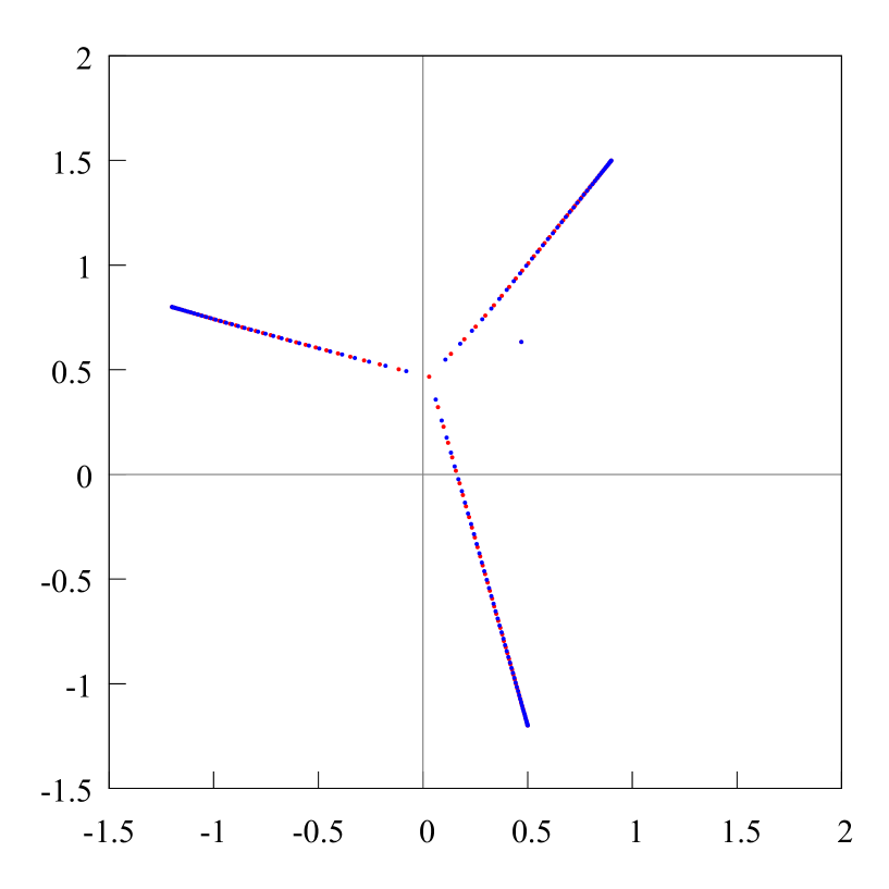
Figure 1. Zeros (blue points) and poles (red points) of PA $[130/130]_{f}$ of the function $f(z)=\bigl{(}z-(-1.2+0.8i)\bigr{)}^{1/3}\bigl{(}z-(0.9+1.5i)\bigr{)}^{1/3}\bigl{(}z-(0.5-1.2i)\bigr{)}^{-2/3}$. Since the genus of the corresponding Stahl’s two-sheeted Riemann surface equals $1$ (i.e. it is an elliptic Riemann surface), there might be at most a single “spurious” zero-pole pair, i.e. a single Froissart doublet. It is really present on the picture.

Conjectures 1 and 2 are based on the rigorous results from [38, Theorem 1.8] and [58], as well as on the numerical experiments produced by the authors in [26], [27]; for more details see §3.4 and Fig. 1–14.

2. Padé approximants

2.1. Padé approximants and $J$-fractions

Since Hermite approximants are a generalization of classical Padé approximants, we start from the basic definition of Padé polynomials $P_{n,0},P_{n,1}$ and of Padé approximants $[n/n]_{f}:=-P_{n,0}/P_{n,1}$.

We recall the definition of PA of an analytic function, given by the power (in fact, by Laurent) series (1) at the infinity point $z=\infty$. For the sake of convenience, we introduce the Padé polynomials $P_{n,0},P_{n,1}\in\mathbb{C}^{*}_{n}[z]$ in the following way. There exist polynomials $P_{n,0}$ and $P_{n,1}$ of degree $\leqslant{n}$ such that (cf. (2))

$$(P_{n,0}\cdot 1+P_{n,1}\cdot f)(z)=O\left(\frac{1}{z^{n+1}}\right),\quad z\to\infty.$$ (7)

The rational function $-P_{n,0}/P_{n,1}$ is uniquely determined and is called the diagonal Padé approximant $[n/n]_{f}=-P_{n,0}/P_{n,1}$ of the function $f$ (at the infinity point).

In the “generic case” the relation (7) is equivalent to the relation

$$\bigl{(}f-[n/n]\bigr{)}(z)=O\left(\frac{1}{z^{2n+1}}\right),\quad z\to\infty.$$ (8)

Thus, from (8) follows that the $n$-th PA $[n/n]_{f}$ is the best local rational approximant of order $\leqslant{n}$ of the given power series (1). Notice that $[n/n]_{f}$ is a rational function with free poles and free zeros. Furthermore, it interpolates the given power series $f$ at the fixed point $z=\infty$ up to the order $2n+1$. Hence,

$$[n/n]_{f}(z)=c_{0}+\frac{c_{1}}{z}+\dots+\frac{c_{2n}}{z^{2n}}+O\left(\frac{1}{z^{2n+1}}\right),\quad z\to\infty.$$ (9)

Recall that by definition of the partial sums $S_{2n}(z)$ of the power series (1)

$$S_{2n}(z)=c_{0}+\frac{c_{1}}{z}+\dots+\frac{c_{2n}}{z^{2n}},$$ (10)

that is,

$$[n/n]_{f}(z)-S_{2n}(z)=O\left(\frac{1}{z^{2n+1}}\right),\quad z\to\infty.$$

Relations (9) and (10) together lead to a very natural question, namely: do the PA $[n/n]_{f}(z)$ have some real advantages over the partial sums $S_{2n}(z)$?

The answer is “yes” and comes from the classical $J$-fractions theory. This is the well-known classical way to evaluate an analytic function going out from its germ, a way which goes back to Gauss and Jacoby (see [6]). However, they used it to evaluate only special (in particular, hypergeometric) functions.

Recall that $f$ is a multivalued analytic function with a finite set $\Sigma$ of branch points, $\operatorname{card}\Sigma<\infty$. To be more precise, we suppose that $f$ is analytic in the domain $\overline{\mathbb{C}}\setminus\Sigma$, but not holomorphic in $\overline{\mathbb{C}}\setminus\Sigma$. We adopt the notation $f\in\mathscr{A}^{\circ}(\overline{\mathbb{C}}\setminus\Sigma):=\mathscr{A}(\overline{\mathbb{C}}\setminus\Sigma)\setminus\mathscr{H}(\overline{\mathbb{C}}\setminus\Sigma)$.

Let $Q\in\mathbb{C}[z]$ be an arbitrary complex polynomial. We denote the zero-counting measure of the polynomial $Q$ by $\chi(Q)$, that is,

$$\chi(Q):=\sum_{\zeta:Q(\zeta)=0}\delta_{\zeta},$$ (11)

where the zeros of $Q$ are counted with regards to their multiplicities; as usual, $\delta_{\zeta}$ denotes the Dirac measure, concentrated at the point $\zeta\in\overline{\mathbb{C}}$.

Let $f\in\mathscr{L}$ be in a “generic case”.

Then we can use the functional analog of Euclid’s algorithm to obtain the formal expansion (see [16], [6])

$$f(z) =1+\frac{A_{1}}{z-B_{1}-f_{1}(z)}=1+\frac{A_{1}}{z-B_{1}-\dfrac{A_{2}}{z-B_{2}-f_{2}(z)}}$$

$$\simeq 1+{\frac{{A_{1}}\vphantom{b}\hfill}{z-B_{1}-\dfrac{A_{2}\vphantom{b}\hfill}{z-B_{2}-\dfrac{A_{3}\qquad\vphantom{b}\hfill}{\begin{smallmatrix}\\ \ddots\end{smallmatrix}}}}}\simeq J(z),$$

where all $A_{n}$ do not vanish, $A_{n}\neq 0$, $n=2,3,\dotsc$. As usual, the notation “$\simeq$” means only a formal equality with no convergence statements. Thus let us consider the $n$-th truncate $J_{n}(z)$ of the continued fraction $J(z)$, i.e.

$$J_{n}(z):=1+\frac{A_{1}\vphantom{b}\hfill}{z-B_{1}-\dfrac{A_{2}\vphantom{b}\hfill}{z-B_{2}-\dfrac{A_{3}\qquad\vphantom{b}\hfill}{\dfrac{\qquad\ddots\qquad}{z-B_{n-1}-\dfrac{A_{n}}{z-B_{n}}}.}}}$$

We recall that $J_{n}$ is a rational function of order $n$, $J_{n}\in\mathbb{C}_{n}(z)$. Set $J_{\infty}(z):=\lim\limits_{n\to\infty}J_{n}(z)$. The problem of convergence of the $J$-fraction to $f$ may be stated as the problem of equality

$$f(z)\overset{\text{?}}{=}J_{\infty}(z),$$ (12)

in other words, it is the problem of evaluation of $f(z)$ via $J_{\infty}(z)$. Since $f$ is a multivalued function and all the $J_{n}$ are single valued functions, two main questions arise in connection with Problem (12): in what sense this equality might be understood and in what domain does it hold true?

2.2. Problem of equality $f(z)=J_{\infty}(z)$: case $p=2$

Let in (3) $p=2$, i.e.

$$f(z)=\left(\frac{z+1}{z-1}\right)^{\alpha},\quad\alpha\in\mathbb{C}\setminus\mathbb{Z}.$$ (13)

Let assume that $\alpha\in(-1/2,1/2)$, $\alpha\neq 0$. Then for $Q_{n}$, where $J_{n}=P_{n}/Q_{n}$, we easily obtain (see [16], [59])

$$\int_{-1}^{1}Q_{n}(x)\,x^{k}\left(\frac{1+x}{1-x}\right)^{\alpha}\,dx=0,\quad k=0,\dots,n-1.$$ (14)

Thus $Q_{n}(x)=P^{(-\alpha,\alpha)}_{n}(x)$ is the Jacobi polynomial of degree $n$ with the parameters $(-\alpha,\alpha)$, $\alpha\in(-1/2,1/2)$, and orthogonal on $E=[-1,1]$. It follows immediately from (14) that all zeros of $Q_{n}$ belong to the segment $[-1,1]$, furthermore, for $\chi(Q_{n})$ the relation

$$\frac{1}{n}\chi(Q_{n})\overset{*}{\longrightarrow}\frac{dx}{\pi\sqrt{1-x^{2}}},\quad n\to\infty.$$ (15)

holds (see (11)). It is well-known that $P^{(-\alpha,\alpha)}_{n}(z)$ solves the following linear differential equation of 2-nd degree

$$(z^{2}-1)w^{\prime\prime}+2(z-\alpha)w^{\prime}-n(n+1)w=0.$$ (16)

By applying the classical asymptotic Liouville–Steklov method [59, § 8.63] to the equation (16), we obtain a formula for the strong asymptotics of the Jacobi polynomials

$$P_{n}^{(-\alpha,\alpha)}(z)=\left(\frac{z-1}{z+1}\right)^{\alpha/2}\frac{(z+(z^{2}-1)^{1/2})^{n+1/2}}{(z^{2}-1)^{1/4}}\left(1+O\left(\frac{1}{n}\right)\right),\quad z\notin\Delta.$$ (17)

Since for the numerator $P_{n}$ of $J_{n}=P_{n}/Q_{n}$ we have $P_{n}=P^{(\alpha,-\alpha)}_{n}$, i.e. $P_{n}$ is Jacobi polynomial of order $n$ with parameters $(\alpha,-\alpha)$, a direct analog of the strong asymptotics formula (17) is also valid for $P_{n}$. Thus after combining them, these two formulae provide a strong asymptotics formula for the rational function $J_{n}$

$$J_{n}(z)=\left(\frac{z+1}{z-1}\right)^{\alpha}\left(1+O\left(\frac{1}{n}\right)\right),\quad z\notin\Delta.$$

Therefore,

$$f(z)=J_{\infty}(z)\quad\text{for}\quad z\in\overline{\mathbb{C}}\setminus\Delta.$$ (18)

2.3. Problem of equality $f(z)=J_{\infty}(z)$: case $p=3$

In 1885 Laguerre [32] made an attempt to solve Problem (12) for the partial case when $p=3$ and $f\in\mathscr{L}$ (cf. (3)), i.e.,

$$f(z)=\prod_{j=1}^{3}(z-a_{j})^{\alpha_{j}},\quad\alpha_{j}\in\mathbb{C}\setminus\mathbb{Z},\quad\sum_{j=1}^{3}\alpha_{j}=0,$$ (19)

where the points $a_{1},a_{2},a_{3}$ are in a “general position”; in particular, they are pairwise distinct and don’t belong to a straight line.

Laguerre derived in 1885 the property of nonhermittian orthogonality for the denominators $Q_{n}$ of the rational function $J_{n}=P_{n}/Q_{n}$, i.e.

$$\oint_{\Gamma}Q_{n}(\zeta)\zeta^{k}f(\zeta)\,d\zeta=0,\quad k=0,\dots,n-1,$$ (20)

where $\Gamma$ is an arbitrary closed contour that separates the three points $a_{1}$, $a_{2}$, $a_{3}$ from the infinity point. He also proved (see also [44], [42], [38]) that the polynomial $P_{n}$ and the function $Q_{n}f$ solve the following linear differential equation of second order

$$A_{3}(z)\Pi_{n,1}(z)w^{\prime\prime}+\Pi_{n,3}(z)w^{\prime}+\Pi_{n,2}(z)w=0,$$ (21)

where $A_{3}(z)=\prod_{j=1}^{3}(z-a_{j})$ and $\Pi_{n,k}\in\mathbb{C}_{k}[z]$, $k=1,2,3$, are some polynomials of degree $k$. To be more precise,

$$\Pi_{n,1}(z) =z-z_{n},$$

$$\Pi_{n,2}(z) =-n(n+1)(z-b_{n})(z-v_{n}),$$

$$\Pi_{n,3}(z) =(z-z_{n})B_{2}(z)-A_{3}(z),\quad B_{2}(z)=A_{3}^{\prime}(z)f^{\prime}(z)/f(z).$$

Thus the polynomial coefficients in equation (21) are of fixed degrees, but depend on $n$. These polynomial coefficients contain three so-called accessory parameters $z_{n},b_{n},v_{n}$, the behavior of which as $n\to\infty$ is presently unknown. That is why Laguerre couldn’t solve neither the problem about the asymptotic behavior of the polynomials $P_{n}$ and $Q_{n}$, nor the Problem about the equality $f(z)=J_{\infty}(z)$ as well.

For case $\Sigma=\{a_{1},a_{2},a_{3}\}$, Problem (12), which is about the strong convergence of $J$-fraction, was solved by J. Nuttall in 1986 only in terms of PA, and on the basis of the seminal Stahl’s Theorem [55] about the convergence in capacity of PA of an arbitrary multivalued analytic function with a finite set of branch points (for the strong asymptotics and strong convergence properties, see also [41], [43], [56], [7], [28], [4]).

In the “generic case” $[n/n]_{f}(z)=J_{n}(z)$. Hence, the Problem about the equality $f(z)=J_{\infty}(z)$ is in fact the problem about the convergence of the sequence of PA $\{[n/n]_{f}(z),n=0,1,\dots\}$ of the given analytic function $f$.

Nuttall proved (see [42]) that for the function $f\in\mathscr{L}$, given by (19), the equality $f(z)=J_{\infty}(z)$ holds true inside the domain $D:=\overline{\mathbb{C}}\setminus{S}$, where $S$ is Stahl’s compact set, up to a unique arbitrary zero-pole pair (in other words, a spurious zero-pole pair, or a Froissart doublet; see [19], [56], [4]). To be more precise, there is a sequence $z_{n}\in\overline{\mathbb{C}}$ such that for each compact set $K\subset{D}$ and for every positive $\varepsilon>0$

$$\sup_{z\in K\setminus\{z:|z-z_{n}|<\varepsilon\}}\bigl{|}f(z)-J_{n}(z)\bigr{|}\to 0,\quad n\to\infty$$ (22)

(cf. (18)). Notice that the convergence relation (22) does not result from Stahl’s Theorem, since it is dealing with the LZD (the Limit Zero Distribution) of Padé polynomials and with the convergence of PA in capacity; for the strong convergence see also [7], [4], [36], [29].

2.4. Classical Padé approximants: Stahl’s Theory

Let $f\in\mathscr{H}(\infty)$ be a multivalued analytic function in the class $\mathscr{A}^{\circ}(\overline{\mathbb{C}}\setminus\Sigma)$, $\operatorname{card}\Sigma<\infty$,

Given a positive Borel measure $\mu$ with a compact support $\operatorname{supp}\mu\subset\overline{\mathbb{C}}$, $\operatorname{supp}\mu\neq\overline{\mathbb{C}}$, let $V^{\mu}(z)$ be the logarithmic potential (see [33], [48]) associated with $\mu$, that is:

$$V^{\mu}(z):=\int_{\operatorname{supp}\mu}\log\frac{1}{|z-\zeta|}\,d\mu(\zeta).$$

We set $V_{*}^{\mu}(z)$ for the spherically normalized logarithmic potential of measure $\mu$, i.e.

$$V_{*}^{\mu}(z):=\int_{|\zeta|\leqslant 1}\log\frac{1}{|z-\zeta|}\,d\mu(\zeta)+\int_{|\zeta|>1}\log\frac{1}{|1-z/\zeta|}\,d\mu(\zeta).$$

Let $f$ be the germ of a multivalued analytic function $f$ with a finite set of branch points. Then the seminal Stahl’s Theorem gives a complete answer to the problem about the limit zero-pole distribution of the classical PA of $f$. The keystone of Stahl’s Theory is the existence of a unique “maximal domain” of holomorphy of $f$, i.e. of a domain $D=D(f)\ni\infty$ such that the given germ $f$ can be continued as a holomorphic (i.e. analytic and single-valued) function from a neighborhood of the infinity point $z=\infty$ into $D$ (i.e. the function $f$ is continued analytically along each path belonging to $D$). “Maximal” means that $\partial{D}$ is of “minimal capacity” among all compact sets $\partial{G}$ such that $G$ is a domain, $G\ni\infty$ and $f\in\mathscr{H}(G)$. To be more precise, we have

$$\operatorname{cap}{\partial D}=\min\{\operatorname{cap}{\partial G}:\,\text{domain}\,G\ni\infty,f\in\mathscr{H}(G)\}.$$

The “maximal” domain $D$ is unique up to an arbitrary compact set of zero capacity.

The compact set $S=S(f):=\partial{D}$ is called “Stahl’s compact set” or “Stahl’s $S$-compact set” and $D$ is called “Stahl’s domain”, respectively. The crucial properties of $S$ for the theory of Stahl to be true are the following: the complement $D=\overline{\mathbb{C}}\setminus{S}$ is a domain, $S$ consists of a finite number of analytic arcs (in fact, the union of the closures of the critical trajectories of a quadratic differential), and finally, $S$ possesses the following property of “symmetry” (compact sets of such type are usually called “$S$-compact sets” or “$S$-curves”, see [45], [30]):

$$\frac{\partial g_{S}(z,\infty)}{\partial n^{+}}=\frac{\partial g_{S}(z,\infty)}{\partial n^{-}},\quad z\in S^{\circ};$$ (23)

where $g_{S}(z,\infty)$ is the Green’s function of the domain $D$ with a logarithmic singularity at the point $z=\infty$, $S^{\circ}$ is the union of all open arcs of $S$ (whose closures constitute $S$, i.e. $S\setminus S^{\circ}$ is a finite set), and $\partial n^{+},\,\partial n^{-}$ mean the inner (with respect to $D$) normal derivatives of $g_{S}(z,\infty)$ at a point $z\in S^{\circ}$ from the opposite sides of $S^{\circ}$. Let $\lambda=\lambda_{S}$ be the unique equilibrium probability measure for $S$, i.e. $V^{\lambda}(z)\equiv\operatorname{const}=\gamma_{S}$ for $z\in S$; $\gamma_{S}$ is the Robin constant for $S$. Then, by the identity $g_{S}(z,\infty)\equiv\gamma_{S}-V^{\lambda}(z)$, the property of symmetry (23) is equivalent to the property

$$\frac{\partial V^{\lambda}}{\partial n^{+}}(z)=\frac{\partial V^{\lambda}}{\partial n^{-}}(z),\quad z\in S^{\circ}.$$ (24)

If

$$f(z)=\prod_{j=1}^{3}(z-a_{j})^{\alpha_{j}},$$

then we have that the compact set $S$ consists of the critical trajectories of the quadratic differential

$$-\frac{z-v}{A_{3}(z)}\,dz^{2}>0,\quad A_{3}(z):=\prod_{j=1}^{3}(z-a_{j}).$$ (25)

These trajectories emanate from the points $a_{j}$ and culminate at the so-called Chebotarëv’s point $z=v$ (see [31]). All points $a_{1},a_{2},a_{3}$ are the simple poles of the quadratic differential (25) and the Chebotarëv point is the simple zero of that differential. In general, Chebotarëv’s point couldn’t be found via elementary functions of the points $a_{1},a_{2},a_{3}$. It is uniquely determined from the condition that both periods of the Abelian integral

$$\int^{z}\sqrt{\frac{\zeta-v}{A_{3}(\zeta)}}\,d\zeta$$ (26)

are purely imaginary. Because of this, the function

$$\Re\int_{a_{1}}^{z}\sqrt{\frac{\zeta-v}{A_{3}(\zeta)}}\,d\zeta$$ (27)

is a single-valued harmonic function on the two-sheeted elliptic Riemann surface $\mathfrak{R}_{2}$, given by the equation $w^{2}=(z-v)A_{3}(z)$. The Chebotarëv–Stahl compact set is given by the equality

$$S=\biggl{\{}z\in\mathbb{C}:\Re\int_{a_{1}}^{z}\sqrt{\frac{\zeta-v}{A_{3}(\zeta)}}\,d\zeta=0\biggr{\}},$$ (28)

and the so-called $g$-function

$$g(z):=\Re\int_{a_{1}}^{z}\sqrt{\frac{\zeta-v}{A_{3}(\zeta)}}\,d\zeta$$ (29)

equals identically to the Green’s function $g_{S}(z,\infty)$ of the domain $D$. From the above results it follows immediately that for the equilibrium measure $\lambda$ (see (25)) the following representation holds:

$$d\lambda(z)=\frac{1}{\pi i}\sqrt{\frac{z-v}{A_{3}(z)}}\,dz>0,\quad z\in S.$$

One of the main results of Stahl’s Theory (see [49]–[53], and also [55]) is

Stahl Theorem (H. Stahl, 1985–1986).

Let the function $f\in\mathscr{H}(\infty)$, $f\in\mathscr{A}^{\circ}(\overline{\mathbb{C}}\setminus\Sigma$), $\operatorname{card}\Sigma<\infty$, let $D=D(f)$ be Stahl’s “maximal” domain of $f$, $S=\partial{D}$ be Stahl’s compact set, and $[n/n]_{f}=-P_{n,0}/P_{n,1}$ be the $n$-th diagonal Padé approximant of the function $f$. Then the following statements are valid:

1) There exists a LZD of Padé polynomials $P_{n,j}$, $j=0,1$, namely,

$$\frac{1}{n}\chi(P_{n,j})\overset{*}{\longrightarrow}\lambda,\quad\text{as}\quad n\to\infty,\quad j=0,1,$$ (30)

where $\lambda=\lambda_{S}$ is the unique probability equilibrium measure for the compact set $S$, i.e. $V^{\lambda}(z)\equiv\gamma_{S}$, $z\in S$, $\gamma_{S}$ – the Robin constant for $S$;

2) the $n$-th diagonal Padé approximants converge in capacity to the function $f$ inside the domain $D$,

$$[n/n]_{f}(z)\overset{\operatorname{cap}}{\longrightarrow}f(z),\quad n\to\infty,\quad z\in D;$$ (31)

3) the rate of the convergence in (31) is completely characterized by the equality

$$\bigl{|}(f-[n/n]_{f})(z)\bigr{|}^{1/n}\overset{\operatorname{cap}}{\longrightarrow}e^{-2g_{S}(z,\infty)},\quad n\to\infty,\quad z\in D.$$ (32)

In fact, for each $f\in\mathscr{A}^{\circ}(\overline{\mathbb{C}}\setminus\Sigma)$ with $\operatorname{card}\Sigma<\infty$, there is only a finite number of the so-called “spurious” zero-pole pairs, or Froissart doublets [19], which makes impossible the pointwise convergence of PA in Stahl’s domain.

The numerical distributions of zeros and poles of PA for the some functions from Laguerre class are demonstrated on the four pictures (see Fig. 1, 2, 3, 4).

2.5. Multipoint Padé approximants: Buslaev’s Theory

Let the set $\Sigma$ with $\operatorname{card}\Sigma<\infty$, the points $z_{k}\in\mathbb{C}\setminus\Sigma$ and functions $f_{k}\in\mathscr{A}^{\circ}(\overline{\mathbb{C}}\setminus\Sigma),\,k=1,\dots,m$ be given. We assume that $f_{j}\in\mathscr{H}(z_{j})$, $j=1,\dots,m$. Let $n\in\mathbb{N}$ be fixed. Then there exists two polynomials $P_{n},Q_{n}\not\equiv 0$ of degrees $\leqslant{n}$ each and such that the following characteristic relations

$$(Q_{n}f_{j}-P_{n})(z_{j})=O\bigl{(}(z-z_{j})^{n_{j}}\bigr{)},\quad z\to z_{j},\quad j=1,\dots,m,$$ (33)

hold, where $\sum_{j=1}^{m}n_{j}=2n+1$, $n_{j}\in\mathbb{Z}_{+}$, $j=1,\dots,m$. Such polynomials $P_{n}$ and $Q_{n}$ are not unique, but the rational function $B_{n}=P_{n}/Q_{n}$ is uniquely determined by the relation (33) and is called a multipoint (or $m$-point) PA of the given set $\mathfrak{f}=\{f_{1},\dots,f_{m}\}$ of the analytic functions $f_{j}\in\mathscr{A}^{\circ}(\overline{\mathbb{C}}\setminus\Sigma)$. In short, we will call the set $\mathfrak{f}=\{(f_{1},z_{1}),\dots,(f_{m},z_{m})\}$ of $m$ multivalued analytic functions $f_{j}\in\mathscr{H}(z_{j})$ the multi-germ or $m$-germ $\mathfrak{f}$.

In general, all functions of the $m$-germ $\mathfrak{f}$ are supposed to be different, i.e. not even one of them, say $f_{j}$, might be obtained as an analytic continuation of another germ, say $f_{k}$, $k\neq j$, along paths, avoiding the set $\Sigma$.

In the generic case, (33) is equivalent to the relation

$$(f_{j}-B_{n})(z)=O\bigl{(}(z-z_{j})^{n_{j}}\bigr{)},\quad z\to z_{j},\quad j=1,\dots,m.$$ (34)

We now suppose that in (33) $n_{j}/n\to 2p_{j}$ as $n\to\infty$, $\sum_{j=1}^{m}p_{j}=1$, $p_{j}\geqslant 0$, $j=1,\dots,m$. According to Buslaev’s Theory (2013–2015; see [11]–[12] and also [13], [14]), there exists (in the nondegenerate case) a unique (up to a set of zero capacity) compact set $F=F_{\operatorname{Bus}}$ which is an $S$-curve weighted in the presence of the external field, which is generated by the unit negative charge $-\nu$, $\nu=\sum_{j=1}^{m}p_{j}\delta_{z_{j}}$ concentrated at the interpolation points $z_{1},\dots,z_{m}$. This compact set possesses the following properties: $F$ consists of a finite number of analytic arcs, the complement $\overline{\mathbb{C}}\setminus F$ of $F$ consists of a finite number of domains $D_{j}\ni z_{j}$, $\overline{\mathbb{C}}\setminus F=\bigcup_{j=1}^{m}D_{j}$; each of the functions $f_{j}$ is holomorphic (i.e. analytic and single-valued) in the corresponding domain $D_{j}$, $f_{j}\in\mathscr{H}(D_{j})$; if for some $k\neq j$ the domains coincide with each other, $D_{j}=D_{k}$, then the corresponding functions are also equal, $f_{k}=f_{j}$; the compact set $F$ possesses the property of “symmetry” in the external field $V_{*}^{-\nu}$. Namely, the following relation holds

$$\frac{\partial(V^{\beta_{F}}-V_{*}^{\nu})}{\partial n^{+}}(z)=\frac{\partial(V^{\beta_{F}}-V_{*}^{\nu})}{\partial n^{-}}(z),\quad z\in{F}^{\circ},$$ (35)

where $\beta_{F}\in M_{1}({F})$ is a unique equilibrium probability measure concentrated on ${F}$ and weighted in $V_{*}^{-\nu}$. In other words, the identity

$$V^{\beta_{F}}(z)-V_{*}^{\nu}(z)\equiv\operatorname{const}=w_{F},\quad z\in{F},$$

is valid, where ${F}^{\circ}$ is the union of all open arcs which closures constitute the compact set $F$; $\partial/\partial n^{\pm}$ are the normal derivatives to ${F}$ at the point $z\in{F}^{\circ}$ from the opposite sides of $F$. It is worth noting that for the fixed $m$-germ $\mathfrak{f}$ the compact set $F$ depends on the numbers $p_{j}\geqslant 0$, $\sum_{j=1}^{m}p_{j}=1$. Therefore, the “optimal” (Buslaev’s) partition of the Riemann sphere into domains $D_{j}$ also depends on $p_{j}$.

Just as in Stahl’s Theory, the existence of the $V^{-\nu}$-weighted $S$-curve $F=F_{\operatorname{Bus}}$ is crucial for Buslaev’s Theory. In accordance with the theory of Stahl, the weighted $S$-property of the compact set $F$ (35) may be expressed in the following way

$$\frac{\partial\biggl{(}\sum\limits_{j=1}^{m}p_{j}g_{D_{j}}(z,z_{j})\biggr{)}}{\partial n^{+}}=\frac{\partial\biggl{(}\sum\limits_{j=1}^{m}p_{j}g_{D_{j}}(z,z_{j})\biggr{)}}{\partial n^{-}},\quad z\in F^{\circ},$$ (36)

where $g_{D_{j}}(z,z_{j})$ is the Green’s function for the domain $D_{j}$ (as usual, we set $g_{D_{j}}(z,z_{j})\equiv 0$ when $z\in D_{k}\neq D_{j}$).

In what follows, for the sake of simplicity, we restrict our attention to the particular case $m=2$ of Buslaev Theorem. Thus, we will discuss in details only the case of two-point Padé approximant.

Let $z_{1}=0$, $z_{2}=\infty$ and $\mathfrak{f}=\{f_{0},f_{\infty}\}$ be the set of two multivalued analytic functions, such that $f_{0}\in\mathscr{H}(0)$ and $f_{\infty}\in\mathscr{H}(\infty)$, and also $f_{0},f_{\infty}\in\mathscr{A}^{\circ}(\overline{\mathbb{C}}\setminus\Sigma)$, where $\operatorname{card}\Sigma<\infty$. Thus, each of the functions $f_{0}$ and $f_{\infty}$ is a multivalued analytic function on the Riemann sphere, punctured at a finite set of points, each of which is a branch point of $f_{0}$ or of $f_{\infty}$ or of both of them. In other words, $f_{0}$ and $f_{\infty}$ are two germs of the multivalued analytic function, given at the point $z_{1}=0$ and $z_{2}=\infty$, respectively. It is worth noting that they may be the two germs of the same analytic function, taken at two different points, namely at $z_{1}=0$ and $z_{2}=\infty$.

The two-point (in the classical terminology, this is the $n$-th truncated fraction of the classical $T$-fraction) PA is defined as follows. Given a number $n\in\mathbb{N}$, let $P_{n},Q_{n}\in\mathbb{C}_{n}[z]$, $Q_{n}\not\equiv 0$, be polynomials of degree $\leqslant{n}$, such that the following relations hold

$$R_{n}(z):=\bigl{(}Q_{n}f-P_{n}\bigr{)}(z)=\begin{cases}O(z^{n}),&z\to 0,\\ O(1/z),&z\to\infty.\end{cases}$$ (37)

The pair of polynomials $P_{n}$ and $Q_{n}$ is not unique, but the rational function $B_{n}:=P_{n}/Q_{n}$ is uniquely determined by (37), and is called the two-point diagonal PA of the set of $2$-germ of the functions $\mathfrak{f}=\{f_{0},f_{\infty}\}$. In the generic case, it follows from (37) that

$$\bigl{(}f-B_{n}\bigr{)}(z)=\begin{cases}O(z^{n}),&z\to 0,\\ O(1/z^{n+1}),&z\to\infty.\end{cases}$$ (38)

If it exists, then the rational function $B_{n}=B_{n}(z;f)\in\mathbb{C}_{n}(z)$ is uniquely determined by the relation (38).

As for the classical Stahl’s case, the existence of an $S$-curve, associated with the two-point PA and weighted in the external field $V_{*}^{-\nu}$, $\nu=(\delta_{0}+\delta_{\infty})/2$, is the crucial element of Buslaev’s two-point convergence theorem. Such a weighted $S$-curve ${F}={F}_{\operatorname{Bus}}(f_{0},f_{\infty})$ exists and realizes the “optimal” partition of the Riemann sphere into two domains $D_{0}\ni 0$ and $D_{\infty}\ni\infty$, such that $\overline{\mathbb{C}}=D_{0}\sqcup{F}\sqcup D_{\infty}$, $f_{0}\in\mathscr{H}(D_{0})$ and $f_{\infty}\in\mathscr{H}(D_{\infty})$. The compact set ${F}$ is a weighted $S$-curve, i.e. ${F}$ consists of a finite number of analytic arcs and possesses the following property of “symmetry”:

$$\frac{\partial(V^{\beta}-V_{*}^{\nu})}{\partial n^{+}}(z)=\frac{\partial(V^{\beta}-V_{*}^{\nu})}{\partial n^{-}}(z),\quad z\in{F}^{\circ},$$ (39)

where $\beta=\beta_{F}$ is the probability measure concentrated on ${F}$ and the equilibrium measure in the external field $V_{*}^{-\nu}(z)=\frac{1}{2}\log|z|$, that is,

$$V^{\beta}(z)-V_{*}^{\nu}(z)\equiv\operatorname{const},\quad z\in{F}$$ (40)

(In fact, the equilibrium measure $\beta$ is generated by the negative unit charge $-\nu$, $\nu=(\delta_{0}+\delta_{\infty})/2$). As before, ${F}^{\circ}$ is the union of all open arcs of ${F}$ (the closures of which constitute ${F}$) and $\partial n^{+}$ and $\partial n^{-}$ are the inner (with respect to $D_{0}$ and $D_{\infty}$) normal derivatives at a point $z\in{F}^{\circ}$ from the opposite sides of ${F}^{\circ}$. Clearly, $\beta$ is the balayage of the measure $\nu$ from $D_{0}\sqcup D_{\infty}$ onto ${F}$. It is worth noting that ${F}$ itself is a union of the closures of the critical trajectories of a quadratic differential and the weighted equilibrium measure $\beta=\beta_{F}$ is given by (see [10])

$$d\beta(\zeta)=\frac{1}{2\pi i}\frac{1}{\zeta}\sqrt{\frac{V_{p}(\zeta)}{A_{p}(\zeta)}}\,d\zeta>0,\quad\zeta\in F.$$ (41)

Here, for the sake of simplicity, we only consider the case of two-point PA, and we set $z_{1}=0$ and $z_{2}=\infty$. In what follows, we also suppose that $f_{0}$ and $f_{\infty}$ are the germs of the same multivalued analytic function $f$, and we denote them by $f_{0}\in\mathscr{H}(0)$ and $f_{\infty}\in\mathscr{H}(\infty)$. We suppose that the function $f$ has a finite set of singular points in $\overline{\mathbb{C}}$.

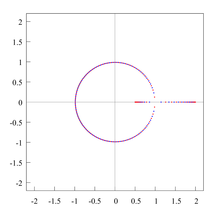
Figure 5. Numerical zeros (blue points) and poles (red points) distribution of two-point PA $[120/120]_{\mathfrak{f}}$ of the set of functions $\mathfrak{f}=\{f_{0},f_{\infty}\}$, where $f_{0}=((1-2z)(2-z))^{-1/2}$, $f_{0}\in\mathscr{H}(0)$, $f_{\infty}=((2z-1)(z-2))^{-1/2}+1$, $f_{\infty}\in\mathscr{H}(\infty)$. The germs $f_{0}$ and $f_{\infty}$ result in two different multivalued analytic functions. Thus, this is a generic case and by Buslaev’s Theorem the associated weighted $S$-curve divides the Riemann sphere into two domains.

Notice that the functions $f_{0}(z)=(1-z^{2})^{-1/2}\sim 1$, $z\to 0$, and $f_{\infty}=(z^{2}-1)^{-1/2}\sim 1/z$, $z\to\infty$, are the germs of the same analytic function $f$, given by the equation $(z^{2}-1)w^{2}=1$. But the functions $f_{0}(z)=(1-z^{2})^{-1/2}$ and $f_{\infty}=(z^{2}-1)^{-1/2}+1$ are not so. Thus, the latter case is the generic case, and hence $D_{0}\cap D_{\infty}=\varnothing$ (see Fig. 5, 6).

Now we are ready to formulate the particular case of Buslaev Theorem for two-point PA (cf. Stahl Theorem).

Buslaev Two-Point Theorem (V. I. Buslaev, 2013–2015).

Let the function $f\in\mathscr{H}(0)\cap\mathscr{H}(\infty)$, $f\in\mathscr{A}^{\circ}(\overline{\mathbb{C}}\setminus\Sigma)$, $\operatorname{card}\Sigma<\infty$, and let the pair of germs $f_{0},f_{\infty}$ be in a general position. Let $D_{0}\sqcup{F}\sqcup D_{\infty}=\overline{\mathbb{C}}$ be the optimal partition of the Riemann sphere into two domains $D_{0}\ni 0$ and $D_{\infty}\ni\infty$, such that $f_{0}\in\mathscr{H}(D_{0})$, $f_{\infty}\in\mathscr{H}(D_{\infty})$, $D_{0}\cap D_{\infty}=\varnothing$, and ${F}$ possesses the weighted $S$-property with respect to the external field $V_{*}^{-\nu}$, $\nu=(\delta_{0}+\delta_{\infty})/2$. Then for the $n$-diagonal two-point PA $B_{n}$ of the set of the germs $\mathfrak{f}=\{f_{0},f_{\infty}\}$ the following statements hold true:

1) there exists a limit zero-pole distribution for $B_{n}$, namely,

$$\frac{1}{n}\chi(P_{n}),\frac{1}{n}\chi(Q_{n})\overset{*}{\longrightarrow}\beta_{F},\quad n\to\infty;$$ (42)

2) there is a convergence in capacity as $n\to\infty$, namely,

$$B_{n}(z)\overset{\operatorname{cap}}{\longrightarrow}f_{0}(z),\quad z\in D_{0},\quad B_{n}(z)\overset{\operatorname{cap}}{\longrightarrow}f_{\infty}(z),\quad z\in D_{\infty};$$ (43)

3) the rate of the convergence in (43) is completely characterized by the relations

$$\bigl{|}f_{0}(z)-B_{n}(z)\bigr{|}^{1/n} \overset{\operatorname{cap}}{\longrightarrow}e^{-g_{D_{0}}(z,0)},\quad z\in D_{0},$$ (44)

$$\bigl{|}f_{\infty}(z)-B_{n}(z)\bigr{|}^{1/n} \overset{\operatorname{cap}}{\longrightarrow}e^{-g_{D_{\infty}}(z,\infty)},\quad z\in D_{\infty}.$$

3. Hermite–Padé polynomials and Hermite approximants

3.1. Definition and uniqueness of Hermite approximants

Let us now suppose that the functions $1,f,f^{2}$ are rationally independent and let us consider type I HP polynomials, i.e. $Q_{n,0},Q_{n,1},Q_{n,2}\in\mathbb{C}_{n}^{*}[z]$ and

$$(Q_{n,0}\cdot 1+Q_{n,1}\cdot f+Q_{n,2}\cdot f^{2})(z)=O\left(\frac{1}{z^{2n+2}}\right),\quad z\to\infty.$$ (45)

We are now facing two very natural questions. What kind of new results come out from Hermite–Padé polynomials? What can be said about the ratios $Q_{n,0}/Q_{n,2}$ and $Q_{n,1}/Q_{n,2}$ (cf. (7)), do they converge to analytic functions corresponding with the given $f$ in some way, or do they not? If yes, then does the sequence $\mathcal{H}_{n,0}(z):=-Q_{n,0}/Q_{n,2}$ provide more detailed information about the analytic properties of the function $f$ than the sequence of Padé approximants $[n/n]_{f}(z)=-P_{n,0}/P_{n,1}$? In general, the answer is unknown. However, in some special cases the answer is positive and appears to be very unusual for the HP polynomials theory. Hence, this problem is very promising for forthcoming investigations.

Lemma 1.

Let two triples of polynomials $Q_{n,0}$, $Q_{n,1}$, $Q_{n,2}\in\mathbb{C}_{n}^{*}[z]$ and $\widetilde{Q}_{n,0}$, $\widetilde{Q}_{n,1}$, $\widetilde{Q}_{n,2}\in\mathbb{C}_{n}^{*}[z]$ satisfy relation (45). Then the following equalities

$$\frac{Q_{n,0}}{\widetilde{Q}_{n,0}}(z)\equiv\frac{Q_{n,1}}{\widetilde{Q}_{n,1}}(z)\equiv\frac{Q_{n,2}}{\widetilde{Q}_{n,2}}(z).$$ (46)

are true.

Proof of Lemma 1.

Indeed, the conditions of Lemma 1 yield

$$(\widetilde{Q}_{n,0}\cdot 1+\widetilde{Q}_{n,1}\cdot f+\widetilde{Q}_{n,2}\cdot f^{2})(z)=O\left(\frac{1}{z^{2n+2}}\right),\quad z\to\infty.$$ (47)

After multiplying both sides of (45) by $\widetilde{Q}_{n,2}$ and both sides of (47) by ${Q}_{n,2}$, respectively and subtracting the new equations, we come to

$$(Q_{n,0}\widetilde{Q}_{n,2}-\widetilde{Q}_{n,0}Q_{n,2})(z)+(Q_{n,1}\widetilde{Q}_{n,2}-\widetilde{Q}_{n,1}Q_{n,2})(z)f(z)=$$

$$=O\left(\frac{1}{z^{n+2}}\right),\quad z\to\infty.$$ (48)

Just in the same way we obtain the equality

$$(\widetilde{Q}_{n,0}Q_{n,1}-Q_{n,0}\widetilde{Q}_{n,1})(z)+(Q_{n,1}\widetilde{Q}_{n,2}-\widetilde{Q}_{n,1}Q_{n,2})(z)f^{2}(z)=$$

$$=O\left(\frac{1}{z^{n+2}}\right),\quad z\to\infty.$$ (49)

It follows immediately from (3.1) and (3.1) that the polynomial

$$P_{2n}:=(Q_{n,1}\widetilde{Q}_{n,2}-\widetilde{Q}_{n,1}Q_{n,2})\in\mathbb{C}_{2n}[z],$$

being of degree $\leqslant{2n}$, is in fact a type II HP polynomial for the pair $f,f^{2}$. Since under the conditions of Lemma 1 the triple $1,f,f^{2}$ is rationally independent over the field $\mathbb{C}(z)$, it follows that in both relations (3.1) and (3.1) the order of approximation at the infinity point should be $O(1/z^{n+1})$ and not $O(1/z^{n+2})$, unless $P_{2n}\equiv 0$. Lemma 1 is proved. ∎

Definition 1.

In what follows, we call the uniquely defined rational functions $Q_{n,0}/Q_{n,2}$ and $Q_{n,1}/Q_{n,2}$ the Hermite Approximants (HA) $\mathcal{H}_{n,0}$ and $\mathcal{H}_{n,1}$, respectively.

3.2. Some theoretical results about Hermite approximants

Suppose that $f\in\mathscr{L}$. Let $Q_{nj},\,j=1,2,3$ be the HP polynomials for the collection $[1,f,f^{2}]$, and $\mathcal{H}_{n,0},\mathcal{H}_{n,1}$ be the corresponding HA of the function $f$.

The case (see (3)) $p=2$ and $a_{1}=-1$, $a_{2}=1$,

$$f(z)=\left(\frac{z+1}{z-1}\right)^{\alpha},\quad f(\infty)=1,$$

where $2\alpha\in\mathbb{R}\setminus\mathbb{Z}$, was treated by A. Martínez-Finkelshtein, E. A. Rakhmanov and S. P. Suetin, 2014–2015 (see [37], [38]). It was proven [38, Theorem 1.8] that for $z\in\mathbb{C}\setminus{F}$ and $F:=\overline{\mathbb{R}}\setminus[-1,1]$, we have for $n\to\infty$ (cf. (5) and (6))

$$\frac{Q_{n,1}}{Q_{n,2}}(z) \to-2\cos{\alpha\pi}\left(\frac{1+z}{1-z}\right)^{\alpha},\quad z\notin{F},$$ (50)

$$\frac{Q_{n,0}}{Q_{n,2}}(z) \to\left(\frac{1+z}{1-z}\right)^{2\alpha}=f^{2}(z),\quad z\notin{F},\quad f(0)=1.$$

Let now $f\in\mathscr{L}$ be given by the representation

$$f(z)=\prod_{j=1}^{q}\left(\frac{z-e_{2j-1}}{z-e_{2j}}\right)^{\alpha}=\left(\prod_{j=1}^{q}\frac{z-e_{2j-1}}{z-e_{2j}}\right)^{\alpha},\quad f(\infty)=1,\quad\alpha\in\mathbb{R}\setminus\mathbb{Z},$$ (51)

with $e_{j}\in\mathbb{R}$, $-1=e_{1}<\dots<e_{2q}=1$. We set $\mathscr{L}_{\mathbb{R}}$ for this subclass of $\mathscr{L}$. Notice that for $f\in\mathscr{L}_{\mathbb{R}}$ the pair $f,f^{2}$ forms the so-called Nikishin’s system (see [39], [40], [22], [18], [3], [34]).

Set $E:=\bigsqcup_{j=1}^{q}[e_{2j-1},e_{2j}]$, $D:=\overline{\mathbb{C}}\setminus{E}$. Since $E=S$ is the Stahl’s compact set for the function $f$ under consideration, then by Stahl’s Theorem

$$[n/n]_{f}(z)\overset{\operatorname{cap}}{\longrightarrow}f(z),\quad n\to\infty,\quad z\in D,$$ (52)

and

$$\bigl{|}f(z)-[n/n]_{f}(z)\bigr{|}^{1/n}\overset{\operatorname{cap}}{\longrightarrow}e^{-2g_{E}(z,\infty)}=e^{2\left(\gamma_{E}-V^{\lambda}(z)\right)},\quad n\to\infty,\quad z\in D,$$ (53)

where $g_{E}(z,\infty)\equiv\gamma_{E}-V^{\lambda}(z)$ is the Green’s function of $D$, $\lambda=\lambda_{E}$ is the unique equilibrium measure of $E$, i.e. $V^{\lambda}(x)\equiv\operatorname{const}$, $x\in E$.

Let now $f_{2}(z)=\operatorname{const}\cdot f(z)$, $\operatorname{const}\neq 0$, be another “branch” (see [17]) of the function $f$, which is holomorphic in the domain $G:=\overline{\mathbb{C}}\setminus F$, where $F:=\overline{\mathbb{R}}\setminus E$, that is, $G\neq D$. In general, if $f\in\mathscr{L}$ is given by the equality $f(z)=\prod\limits_{j=1}^{p}(z-a_{j})^{\alpha_{j}}$, then both functions $f_{1}=f$ and $f_{2}$ solve the same differential equation

$$A_{p}(z)w^{\prime}+B_{p-2}(z)w=0,$$

where

$$A_{p}(z)=\prod_{j=1}^{p}(z-a_{j})\ \text{ and }\ B_{p-2}(z)=-A_{p}(z)\sum_{j=1}^{p}\alpha_{j}(z-a_{j})^{-1}$$

are polynomials of degrees $p$ and $p-2$, respectively. If $p=2$, $a_{1}=-1$, $a_{2}=1$,

$$f(z):=\left(\frac{z+1}{z-1}\right)^{\alpha},\quad z\notin E=[-1,1],\quad f(\infty)=1,$$

then we have

$$f_{2}(z)=-2\cos\alpha\pi\left(\frac{1+z}{1-z}\right)^{\alpha},\quad z\notin F,\quad f_{2}(0)=1;$$

see A. Martínez-Finkelshtein, E. Rakhmanov and S. Suetin [38].

In wider sense, the following result is valid [58] (cf. [35]).

Theorem 1 ((S. Suetin, 2015)).

Let $f$ be of type (51) where $\alpha\in(-1/2,1/2)$, $\alpha\neq 0$, $-1=e_{1}<\dots<e_{2{q}}=1$. Then

1) all zeros of $Q_{n,0}$, $Q_{n,1}$ and $Q_{n,2}$, up to a finite number that is fixed and independent of $n$, belong to $F$; there exists a LZD of HP $Q_{n,j}$:

$$\frac{1}{n}\chi(Q_{n,j})\overset{*}{\longrightarrow}\eta^{\vphantom{p}}_{F},\quad n\to\infty,$$ (54)

$$\text{where}\quad 3V_{*}^{\eta^{\vphantom{p}}_{F}}(y)+G^{\eta^{\vphantom{p}}_{F}}_{E}(y)+3g_{E}(y,\infty)\equiv\operatorname{const},\quad y\in F,\quad\operatorname{supp}\eta^{\vphantom{p}}_{F}=F;$$ (55)

2) the rational function $\mathcal{H}_{n,1}:=-Q_{n,1}/Q_{n,2}$ interpolates the function $f_{2}$ at least at $2n-m$ distinct (“free”) nodes $x_{n,j}$ of $E^{\circ}:=\bigsqcup_{j=1}^{q}(e_{2j-1},e_{2j})$ where $m\in\mathbb{N}$ does not depend on $n$, and there exist LZD of those free nodes $x_{n,j}$, namely

$$\frac{1}{2n}\sum_{j=1}^{2n-m}\delta_{x_{n,j}}\overset{*}{\longrightarrow}\eta^{\vphantom{p}}_{E},\quad n\to\infty,$$ (56)

$$\text{where}\quad 3V^{\eta^{\vphantom{p}}_{E}}(x)+G^{\eta^{\vphantom{p}}_{E}}_{F}(x)\equiv\operatorname{const},\quad x\in E,\quad\operatorname{supp}\eta^{\vphantom{p}}_{E}=E;$$ (57)

3) in the domain $G:=\overline{\mathbb{C}}\setminus{F}$, the following relation is valid

$$\mathcal{H}_{n,1}(z)\overset{\operatorname{cap}}{\longrightarrow}f_{2}(z),\quad z\in G,\quad n\to\infty;$$ (58)

and the rate of convergence is completely characterized by the relations (cf. (53))

$$\bigl{|}f_{2}(z)-\mathcal{H}_{n,1}(z)\bigr{|}^{1/n} \overset{\operatorname{cap}}{\longrightarrow}e^{-2G_{F}^{\eta^{\vphantom{p}}_{E}}(z)}<1,\quad z\in G\setminus{\mathbb{R}},\quad n\to\infty,$$ (59)

$$\varlimsup_{n\to\infty}\bigl{|}f_{2}(x)-\mathcal{H}_{n,1}(x)\bigr{|}^{1/n} \leqslant e^{-2G_{F}^{\eta^{\vphantom{p}}_{E}}(x)}<1,\quad x\in E^{\circ},$$ (60)

where the measure $\eta^{\vphantom{p}}_{E}$ solves problem (57).

In Theorem 1

$$G_{F}^{\eta^{\vphantom{p}}_{E}}(z)=\int_{E}g_{E}(x,z)\,d\eta_{E}(x)$$

is the Green potential of the measure $\eta_{E}$, $\operatorname{supp}\eta_{E}=E$, $g_{E}(x,z)$ is the Green function for $D:=\overline{\mathbb{C}}\setminus{E}$,

$$G_{E}^{\eta^{\vphantom{p}}_{F}}(z)=\int_{F}g_{F}(x,z)\,d\eta_{F}(x)$$

is Green potential of measure $\eta_{F}$, $\operatorname{supp}\eta_{F}\subset F$, $g_{F}(x,z)$ is the Green function for $G:=\overline{\mathbb{C}}\setminus{F}$.

Notice that the equilibrium problem (55) was introduced by S. Suetin and E. Rakhmanov in [46] (see also [57], [9], [15]) and is different from the problem that was studied before in papers [20], [39], [21], [23]; see also [40] and [22].

The case when we have (51) with $q=1$ and $e_{1}=-1$, $e_{2}=1$, that is,

$$f(z)=\left(\frac{z+1}{z-1}\right)^{\alpha},\quad f(\infty)=1,$$

where $2\alpha\in\mathbb{C}\setminus\mathbb{Z}$, was treated by A. Martínez-Finkelshtein, E. A. Rakhmanov and S. P. Suetin in 2013–2015. The first version of Theorem 1 was established in [38, Theorem 1.8]; furthermore, the following explicit representation for both measures $\eta_{E}$ and $\eta_{F}$ were found, namely

$$\frac{d\eta_{F}}{dx}(x) =\frac{\sqrt{3}}{2\pi}\frac{1}{\sqrt[3]{x^{2}-1}}\biggl{(}\frac{1}{\sqrt[3]{|x|-1}}-\frac{1}{\sqrt[3]{|x|+1}}\biggr{)},\quad x\in\overline{\mathbb{R}}\setminus[-1,1],$$

$$\frac{d\eta_{E}}{dx}(x) =\frac{\sqrt{3}}{4\pi}\frac{1}{\sqrt[3]{1-x^{2}}}\biggl{(}\frac{1}{\sqrt[3]{1-x}}+\frac{1}{\sqrt{1+x}}\biggr{)},\quad x\in(-1,1).$$

Recall the explicit representation of Chebyshëv–Robin equilibrium probability measure $\lambda_{\operatorname{cheb}}$ for the unit segment $[-1,1]$:

$$\frac{d\lambda_{\operatorname{cheb}}}{dx}=\frac{1}{\pi\sqrt{1-x^{2}}},\quad x\in(-1,1).$$

Under the condition $\alpha=1/3$, i.e. for the function

$$f(z)=\left(\frac{z+1}{z-1}\right)^{1/3}$$

relation (60) from Theorem 1 might be improved in the following form. The Hermite approximation $\mathcal{H}_{n,1}(z):=-Q_{n,1}/Q_{n,2}(z)$ possesses the property of “almost Chebyshëv alternation” on the open interval $(-1,1)$ in the following sense. For each positive and arbitrary small $\theta>0$ on the interval $(-1,1)$ there exist at least $N_{n}=[2n(1-\theta)]$ consecutive points $x_{j}$, $-1<x_{1}<\dots<x_{N_{n}}<1$, such that the following equality holds:

$$f_{2}(x_{j})-\mathcal{H}_{n,1}(x_{j})=(-1)^{j}e^{-2nG_{F}^{\eta_{E}}(x_{j})}\biggl{\{}\frac{2}{3}\sqrt[3]{\frac{1+x_{j}}{1-x_{j}}\,}\,\bigl{(}1+\varepsilon_{n}(x_{j})\bigr{)}\biggr{\}},$$ (61)

where $\varepsilon_{n}(x)\to 0$ as $n\to\infty$ with a geometrical rate locally uniformly in $(-1,1)$. Let

$$w_{n}(z):=e^{2nG_{F}^{\eta_{E}}(x_{j})}\frac{3}{2}\sqrt[3]{\frac{1-x_{j}}{1+x_{j}}\,}$$

be the weight function. Then (61) implies the following weighted equality

$$w_{n}(x_{j})\bigl{(}f_{2}(x_{j})-\mathcal{H}_{n,1}(x_{j})\bigr{)}=(-1)^{j}(1+\varepsilon_{n}(x_{j})),\quad j=1,\dots,N_{n}.$$

3.3. Orthogonality relations

Let $f\in\mathscr{H}(\infty)$,

$$f(z)=\prod_{j=1}^{p}(z-a_{j})^{\alpha_{j}},\quad\alpha_{j}\in\mathbb{C}\setminus\mathbb{Z},\quad\sum_{j=1}^{p}\alpha_{j}=0,$$ (62)

where the points $a_{j}\in\mathbb{C}$ are pairwise distinct, i.e. $a_{j}\neq a_{k}$ when $j\neq k$. Thus $f\in\mathscr{A}^{\circ}(\overline{\mathbb{C}}\setminus\Sigma)$, where $\Sigma=\{a_{1},\dots,a_{p}\}$. We have in the partial case $f\in\mathscr{L}_{\mathbb{R}}$

$$f(z)=\prod_{j=1}^{q}\left(\frac{z-e_{2j-1}}{z-e_{2j}}\right)^{\alpha},\quad\alpha\in\mathbb{R}\setminus\mathbb{Z},$$ (63)

where $-1=e_{1}<\dots<e_{2q}=1$. Let $|\alpha|\in(0,1/2).$ Let $E:=\bigsqcup_{j=1}^{q}[e_{2j-1},e_{2j}]$, $E^{\circ}:=\bigsqcup_{j=1}^{q}(e_{2j-1},e_{2j})$, $E_{j}:=[e_{2j-1},e_{2j}]$.

We fix the branch of $f$ at $z=\infty$ by $f(\infty)=1$ and fix a number $n\in\mathbb{N}$. By definition (7)

$$\int_{\gamma}(P_{n,0}+P_{n,1}f)(\zeta)q(\zeta)\,d\zeta=0\quad\forall q\in\mathbb{C}_{n-1}[\zeta],$$ (64)

where $\gamma$ is an arbitrary contour separating the points $e_{1},\dots,e_{2q}$ from the infinity point. Let $f$ be given by (63); then it follows from (64) that

$$\int_{E}P_{n,1}(x)x^{k}\Delta{f}(x)\,dx=0,\quad k=0,\dots,n-1,$$ (65)

where $\Delta{f}(x):=f^{+}(x)-f^{-}(x)$, $x\in{E}$. Since $\operatorname{const}\cdot\Delta{f}>0$ on $E^{\circ}$ for some $\operatorname{const}\neq 0$, we conclude from (65) that:

1) all but some fixed and independent of $n$ number of zeros of $P_{n,1}$ belong to $E$;

2) by Stahl’s Theorem, there exists LZD of Padé polynomials $P_{n,1}$:

$$\frac{1}{n}\chi(P_{n,1})\overset{*}{\longrightarrow}\lambda,\quad n\to\infty,$$ (66)

where $\lambda=\lambda_{E}$ is a unique equilibrium probability measure concentrated on $E$, i.e.

$$V^{\lambda}(x)\equiv\operatorname{const},\quad x\in E;$$ (67)

$E=S$ is the Stahl’s compact set of $f$. From definition (2) of HP polynomials, we may write

$$\int_{\gamma}(Q_{n,0}+Q_{n,1}f+Q_{n,2}f^{2})(\zeta)q(\zeta)\,d\zeta=0\quad\forall q\in\mathbb{C}_{2n}[\zeta],$$ (68)

where $\gamma$ is an arbitrary closed contour that separates points $e_{1},\dots,e_{2q}$ from the infinity point. From (68) it follows that for $q(z)=P_{n+k,1}(z)=P_{n+k,1}(z;f)$ we have

$$\int_{E}Q_{n,2}(x)P_{n+k,1}(x)\widetilde{f}(x)\Delta{f}(x)\,dx=0,\quad k=1,\dots,n,$$ (69)

where $\widetilde{f}(x):=f^{+}(x)+f^{-}(x)$, $x\in{E}$, and $\operatorname{const}\widetilde{f}(x)\Delta{f}(x)>0$ for $x\in E^{\circ}$ with some $\operatorname{const}\neq 0$.

From (69), it follows (see [58]) that:

1) all but some fixed and independent of $n$ number of zeros of $Q_{n,2}$ belong to $F:=\overline{\mathbb{R}}\setminus{E}$;

2) there exists LZD of HP polynomials $Q_{n,2}$:

$$\frac{1}{n}\chi(Q_{n,2})\overset{*}{\longrightarrow}\eta_{F},\quad n\to\infty,$$

where $\eta_{F}$ is a unique special equilibrium probability measure concentrated on $F$, i.e.

$$3V_{*}^{\eta_{F}}(x)+G_{E}^{\eta_{F}}(x)+\psi(x)\equiv\operatorname{const},\quad x\in F;$$ (70)

here

$$G_{E}^{\mu}(z):=\int g_{E}(\zeta,z)\,d\mu(\zeta),\quad\psi(z):=3g_{E}(z,\infty),$$ (71)

$g_{E}(\zeta,z)$ is the Green function for $D:=\overline{\mathbb{C}}\setminus{E}$. The pair of compact sets $E,F$ forms the so-called Nuttall condenser $\mathscr{N}:=(E,F)=(E;F,\psi)$. We call the corresponding special equilibrium measure $\eta_{F}$ from (71) the Nuttall equilibrium measure (see [46], [57], [29]). For LZD of HP polynomials, the notion of Nuttall’s condenser plays a role, which is very similar to the role played by Stahl’s compact set $S$ in the case of Padé polynomials. In general, if the plates $E,F\not\subset\mathbb{R}$, then they both possess some special “symmetry” property, see [46], [57], [29].

3.4. Discussion of some numerical results

We are going to discuss some numerical examples in order to demonstrate a numerical basis for Conjectures 1 and 2 and for the results of Theorem 1 as well.

From numerical experiments made by R. Kovacheva, N. Ikonomov, and S. Suetin [26], [27], it follows that the distribution of zeros of HP polynomials and the convergence of Hermite approximants itself are very sensitive to the type of branching of multivalued analytic function. More precisely, the situation becomes generally much more complicated, even if all branch points $e_{j}$ still belong to the real line, but in (51) instead of one parameter $\alpha$ we take different parameters $\alpha_{j}$, $\alpha_{j}\in\mathbb{R}\setminus\mathbb{Z}$ (see (4)). To be more precise, let the multivalued analytic function $f$ be given by the explicit representation

$$f(z)=\prod_{j=1}^{q}\left(\frac{z-e_{2j-1}}{z-e_{2j}}\right)^{\alpha_{j}},$$ (72)

where $e_{1}<\dots<e_{2q}$, but $\alpha_{j}\neq\alpha_{k},\,j\neq k$. Let us fix the germ of $f$ by the relation $f(\infty)=1$.

Case 1.

Let $q=3$ and

$$f(z)=\left(\dfrac{z+2.5}{z+1.3}\right)^{1/3}\left(\dfrac{z+0.8}{z-0.8}\right)^{1/3}\left(\dfrac{z-1.3}{z-2.5}\right)^{1/3}.$$ (73)

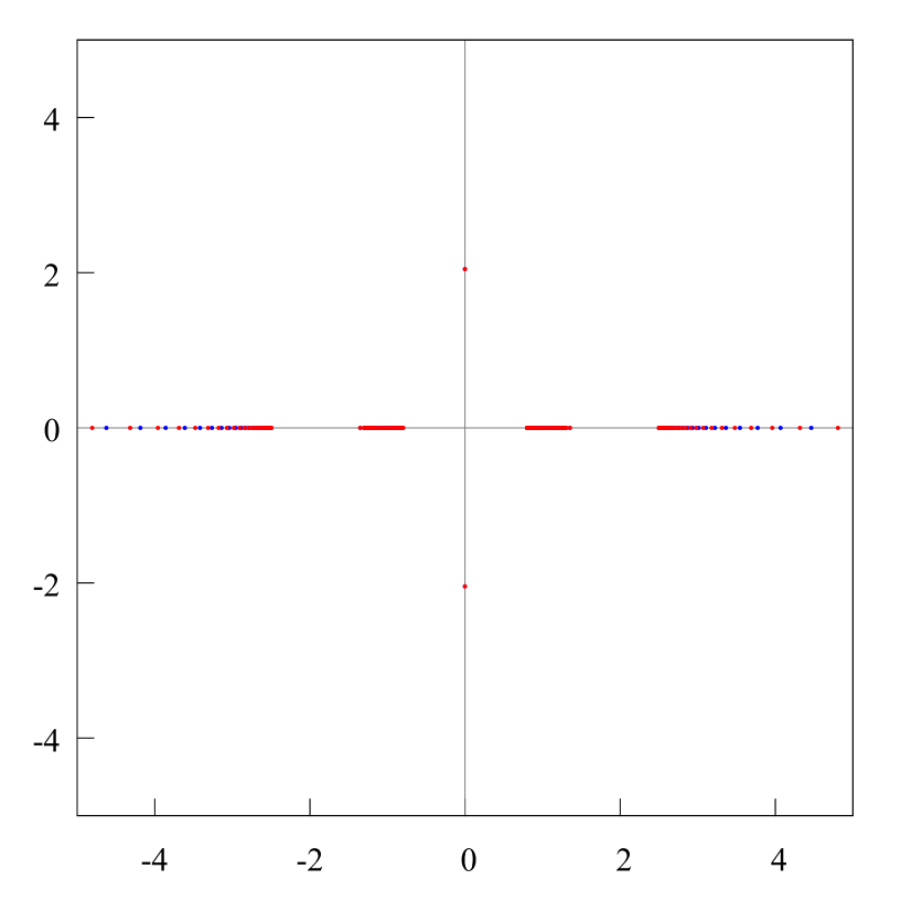
Figure 7. Zeros of HP polynomials $Q_{200,0}$ (blue points) and $Q_{200,1}$ (red points) for the triple of functions $[1,f,f^{2}]$, where $f(z)=\left(\dfrac{z+2.5}{z+1.3}\right)^{1/3}\left(\dfrac{z+0.8}{z-0.8}\right)^{1/3}\left(\dfrac{z-1.3}{z-2.5}\right)^{1/3}$. All but two pairs of zeros are distributed in accordance with Theorem 1 on the real line on the complement of the three closed segments $[-2.5,-1.3]$, $[-0.8,0.8]$, and $[1.3,2.5]$. There are two pairs of complex conjugate Froissart doublets; cf. Fig. 8.

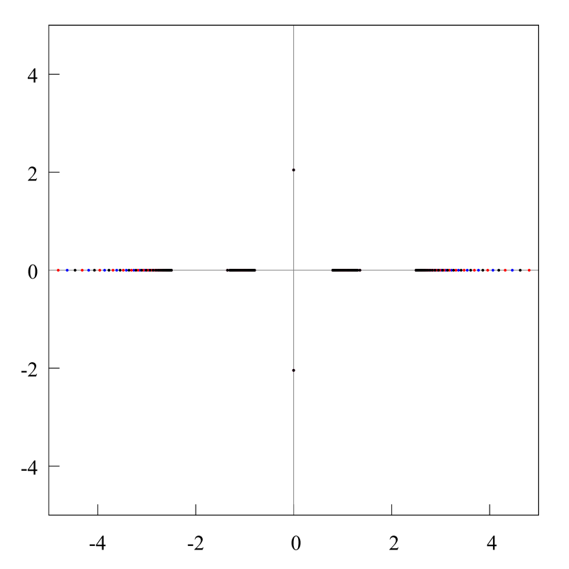
Figure 8. Zeros of HP polynomials $Q_{200,0}$ (blue points), $Q_{200,1}$ (red points), and $Q_{200,2}$ (black points) for the triple of functions $[1,f,f^{2}]$, where $f(z)=\left(\dfrac{z+2.5}{z+1.3}\right)^{1/3}\left(\dfrac{z+0.8}{z-0.8}\right)^{1/3}\left(\dfrac{z-1.3}{z-2.5}\right)^{1/3}$. All but two pairs of zeros are distributed in accordance with Theorem 1 on the real line on the complement of the three closed segments $[-2.5,-1.3]$, $[-0.8,0.8]$, and $[1.3,2.5]$. There are two pairs of complex conjugate Froissart triplets; cf. Fig. 7.

Since in (73) all the exponents are equal to the same $\alpha=1/3$, the zeros of the associated HP polynomials $Q_{200,0}$, $Q_{200,1}$, $Q_{200,2}$ of the collection $[1,f,f^{2}]$ should be distributed in accordance to Theorem 1. From figures 7–8, it follows that it is really the case. All zeros, except a pair of Froissart triplets, are distributed on the real line $\mathbb{R}$ on the complement of three real segments $[-2.5,-1.3]$, $[-0.8,0.8]$, and $[1.3,2.5]$.

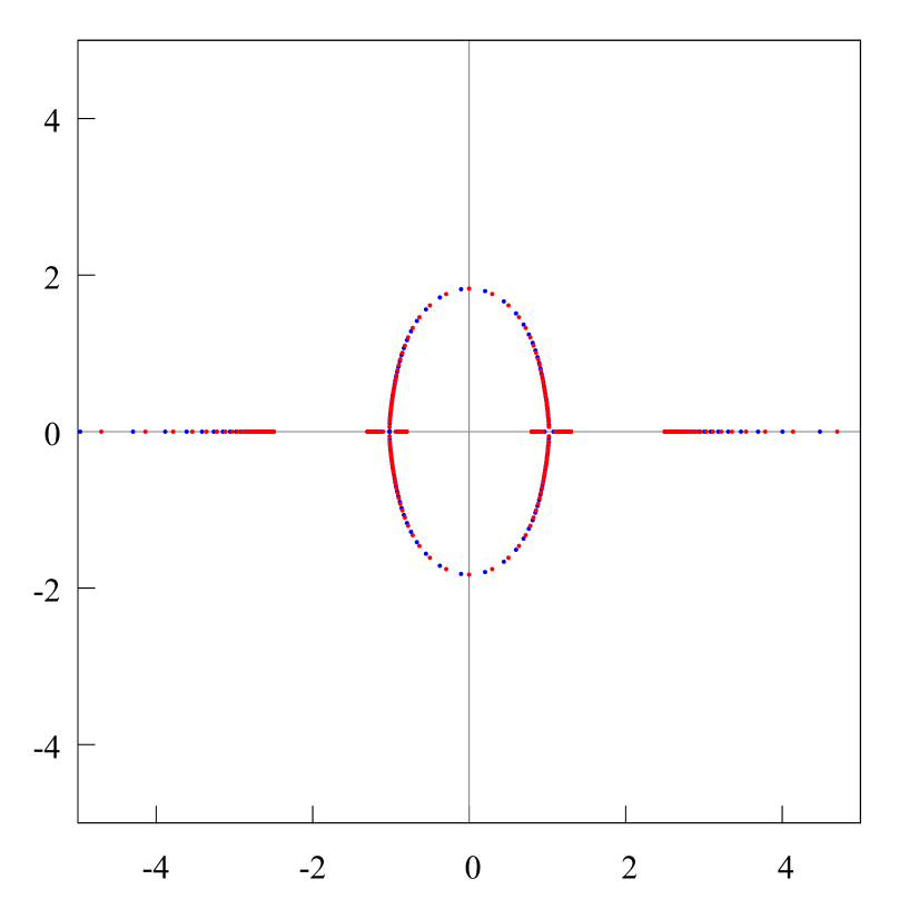
Figure 9. Zeros of HP polynomials $Q_{320,0}$ (blue points) and $Q_{320,1}$ (red points) for the triple of functions for $[1,f,f^{2}]$, where $f(z)=\left(\dfrac{z+2.5}{z+1.3}\right)^{1/3}{\left(\dfrac{z+.8}{z-.8}\right)^{-1/3}}\left(\dfrac{z-1.3}{z-2.5}\right)^{1/3}$. There is a membrane which splits the complement of the segments $[-2.5,-1.3]$, $[-0.8,0.8]$ and $[1.3,2.5]$ into two domains. Both domains are simply connected. The zeros of these HP polynomials are distributed on real line $\mathbb{R}$ on the complement of the segments $[-2.5,-1.3]$, $[-0.8,0.8]$ and $[1.3,2.5]$ and on this membrane. The points of intersection of the membrane with the two segments are the Chebotarëv’s points of zero-density for the equilibrium measure for a compact set $F$. By chance, there are no Froissart doublets at all; cf. Fig. 10.

In the general situation (72), when there are different $\alpha_{j}$ (instead of a single $\alpha$) there should be membranes which separate the segments of the set $F$ (see Fig. 9–14).

Case 2.

Let $q=3$ and

$$f(z)=\left(\dfrac{z+2.5}{z+1.3}\right)^{1/3}\left(\dfrac{z+0.8}{z-0.8}\right)^{-1/3}\left(\dfrac{z-1.3}{z-2.5}\right)^{1/3}.$$ (74)

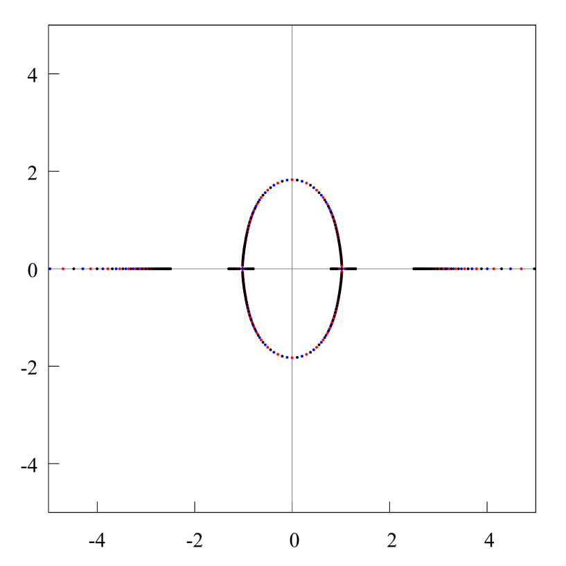
Figure 10. Zeros of HP polynomials $Q_{320,0}$ (blue points), $Q_{320,1}$ (red points), and $Q_{320,2}$ (black points) for the triple of functions for $[1,f,f^{2}]$, where $f(z)=\left(\dfrac{z+2.5}{z+1.3}\right)^{1/3}{\left(\dfrac{z+0.8}{z-.08}\right)^{-1/3}}\left(\dfrac{z-1.3}{z-2.5}\right)^{1/3}$. There is a membrane which splits the complement to the segments $[-2.5,-1.3]$, $[-0.8,0.8]$ and $[1.3,2.5]$ into two domains. Both domains are simply connected. The zeros of these HP polynomials are distributed on real line $\mathbb{R}$ on the complement of the segments $[-2.5,-1.3]$, $[-0.8,0.8]$ and $[1.3,2.5]$ and on this membrane. The points of intersection of the membrane with the two segments are the Chebotarëv’s points of zero-density for the equilibrium measure for a compact set $F$. By chance, there are no Froissart triplets at all; cf. Fig. 9.

Thus in (72) $\alpha_{j}=(-1)^{j+1}\alpha$. Figures 9–10 represent the numerical distribution of zeros of HP polynomials $Q_{320,0}$, $Q_{320,1}$, $Q_{320,2}$ of the collection of the functions $[1,f,f^{2}]$. In this case there is a membrane, which splits the complement of the segments $[-2.5,-1.3]$, $[-0.8,0.8]$ and $[1.3,2.5]$ into two domains. The zeros of these HP polynomials are distributed on the real line $\mathbb{R}$ on the complement of the segments $[-2.5,-1.3]$, $[-.8,.8]$ and $[1.3,2.5]$ and on this membrane. The points of intersection of the membrane with the two segments are the Chebotarëv’s points of zero-density for the equilibrium measure for a compact set $F$. By chance, there are no Froissart triplets at all (see Fig. 9–10).

Case 3.

Let $q=3$ and

$$f(z)=\left(\dfrac{z+2.5}{z+1.3}\right)^{1/3}\left(\dfrac{z+0.3}{z-0.3}\right)^{1/2}\left(\dfrac{z-1.3}{z-2.5}\right)^{-1/3}.$$ (75)

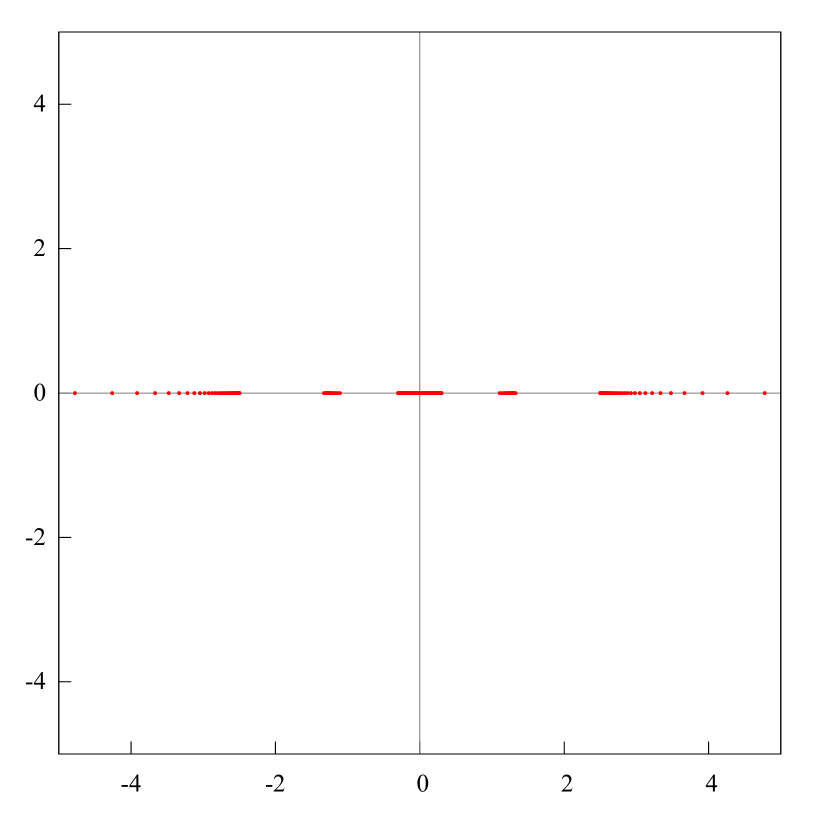
Figure 11. Zeros of HP polynomial $Q_{320,1}$ (red points) for the triple of functions $[1,f,f^{2}]$, where $f(z)=\left(\dfrac{z+2.5}{z+1.3}\right)^{1/3}{\left(\dfrac{z+0.3}{z-0.3}\right)^{1/2}}\left(\dfrac{z-1.3}{z-2.5}\right)^{1/3}$. There is no membrane here. The zeros of HP polynomial $Q_{320,1}$ are distributed on the real line on the complement of four segments $[-2.5,-1.3]$, $[-a,-0.3]$, $[0.3,a]$, and $[1.3,2.5]$ where $a\in(0.3,1.3)$ is an unknown parameter. This parameter should be evaluated from an appropriate theoretical-potential equilibrium problem. By chance, there are no Froissart doublets at all. In case of the given function $f$, the numerical distribution of zeros of HP polynomial $Q_{320,1}$ is very different from numerical distribution of zeros of HP polynomial $Q_{320,0}$ and $Q_{320,2}$; cf. Fig. 12, 13, 14.

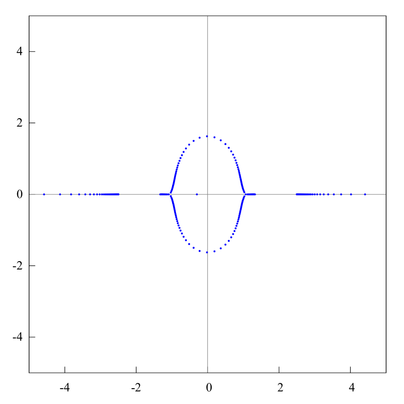
Figure 12. Zeros of HP polynomial $Q_{320,0}$ (blue points) for the triple of functions $[1,f,f^{2}]$, where $f(z)=\left(\dfrac{z+2.5}{z+1.3}\right)^{1/3}{\left(\dfrac{z+0.3}{z-0.3}\right)^{1/2}}\left(\dfrac{z-1.3}{z-2.5}\right)^{1/3}$. There is a membrane which splits the Riemann sphere into two domains. The zeros of HP polynomial $Q_{320,0}$ are distributed on this membrane and on the real line on the complement of three segments $[-2.5,-1.3]$, $[-a,a]$, and $[1.3,2.5]$. The membrane and a parameter $a\in(0.3,1.3)$ come from an appropriate theoretical-potential equilibrium problem. By chance, there are no Froissart doublets at all. In case of the given function $f$, the numerical distribution of zeros of HP polynomial $Q_{320,0}$ is very different from the numerical distribution of zeros of HP polynomial $Q_{320,1}$; cf. Fig. 11 and also 14. There is a zero of polynomial $Q_{320,0}$ inside the membrane which correspond to the simple zero of the function $f^{2}$ at the point $z=-0.3$.

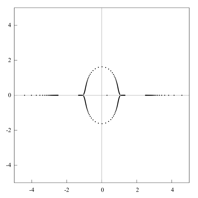
Figure 13. Zeros of HP polynomial $Q_{320,2}$ (black points) for the triple of functions $[1,f,f^{2}]$, where $f(z)=\left(\dfrac{z+2.5}{z+1.3}\right)^{1/3}{\left(\dfrac{z+0.3}{z-0.3}\right)^{1/2}}\left(\dfrac{z-1.3}{z-2.5}\right)^{1/3}$. There is a membrane which splits the Riemann sphere into two domains. The zeros of HP polynomial $Q_{320,2}$ are distributed on this membrane and on the real line on the complement of three segments $[-2.5,-1.3]$, $[-a,a]$, and $[1.3,2.5]$. The membrane and a parameter $a\in(0.3,1.3)$ come from an appropriate theoretical-potential equilibrium problem. By chance, there are no Froissart doublets at all. In case of the given function $f$, the numerical distribution of zeros of HP polynomial $Q_{320,2}$ is very different from the numerical distribution of zeros of HP polynomial $Q_{320,1}$; cf. Fig. 11 and also 14. There is a zero of polynomial $Q_{320,2}$ inside the membrane which correspond to the simple pole of the function $f^{2}$ at the point $z=0.3$.

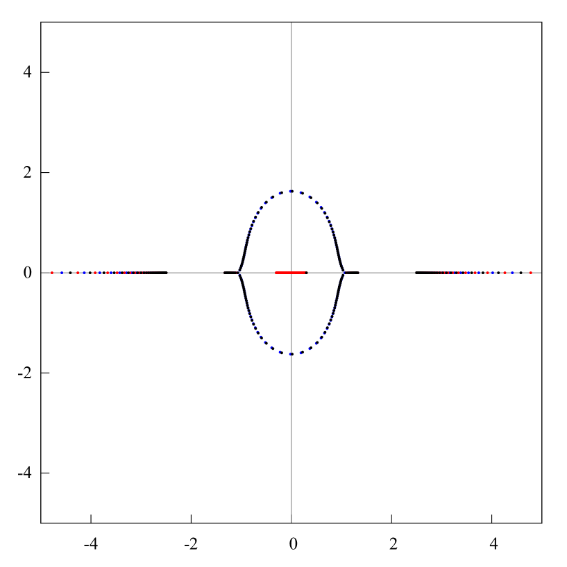
Figure 14. Zeros of HP polynomials $Q_{320,0}$ (blue points), $Q_{320,1}$ (red points), and $Q_{320,2}$ (black points) for the triple of functions $[1,f,f^{2}]$, where $f(z)=\left(\dfrac{z+2.5}{z+1.3}\right)^{1/3}{\left(\dfrac{z+0.3}{z-0.3}\right)^{1/2}}\left(\dfrac{z-1.3}{z-2.5}\right)^{1/3}$. There is a membrane which splits the Riemann sphere into two domains. One domain is simply connected, but the other is a doubly connected domain. The zeros of these HP polynomials are distributed in accordance with the description given in Fig. 11, 12, 13. The points of intersection of the membrane with the two segments $[-1.3,-a]$ and $[a,1.3]$ are the Chebotarëv’s points of zero-density for the equilibrium measure from an appropriate theoretical-potential equilibrium problem. By chance, there are no Froissart doublets at all.

Figures 11–14 represent the numerical distribution of zeros of HP polynomials $Q_{200,0}$, $Q_{200,1}$, $Q_{200,2}$ for the collections of functions $[1,f,f^{2}]$. There also exists a membrane, but of another type than in Case 2. This membrane splits the complement of the three segments $[-2.5,-1.3]$, $[-0.3,0.3]$ and $[1.3,2.5]$ into two domains. The zeros of those HP polynomials are distributed on the real line $\mathbb{R}$ on the complement of the segments $[-2.5,-1.3]$, $[-0.3,0.3]$ and $[1.3,2.5]$ on this new membrane. Just as in Case 2, the two points of intersection of the membrane with the segments are the Chebotarev’s points of zero-density for the equilibrium measure for compact set $F$.

3.5. Final remarks about Hermite approximants

Thus, from the numerical experiments of R. Kovacheva, N. Ikonomov, and S. Suetin, see [26], [27] it follows that the distribution of zeros of HP polynomials for the collection $[1,f,f^{2}]$ and the convergence of Hermite approximants $\mathcal{H}_{n,j}$, $j=0,1$, itself are very sensitive to the type of branching of the given multivalued analytic function $f$. By this reason, it might be very difficult to construct a general theory of limit zero distribution of HP polynomials of such type as Stahl’s and Buslaev’s theories are. But as surplus, this sensitivity makes Hermite approximants $\mathcal{H}_{n,j}$ very powerful tool to recover the unknown properties of a multivalued analytic function given by a germ.

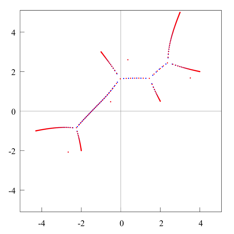
Figure 2. Zeros (blue points) and poles (red points) of PA $[267/267]_{f}$ of the function $f(z)=\{(z+(4.3+1.0i))(z-(2.0+0.5i))(z+(2.0+2.0i))(z+(1.0-3.0i))(z-(4.0+2.0i))(z-(3.0+5.0i))\}^{-1/6}$. These zeros and poles are distributed in a plane, under fixed $n=267$, accordingly to the electrostatic model by Rakhmanov [45]. There are $4$ Chebotarëv points on the picture. Thus the genus of the Stahl’s hyperelliptic Riemann surface is $4$. By this reason for each $n$ there might be no more than $4$ Froissart doublets. Here are observed $4$ Froissart doublets (cf. [58, Fig. 2]).

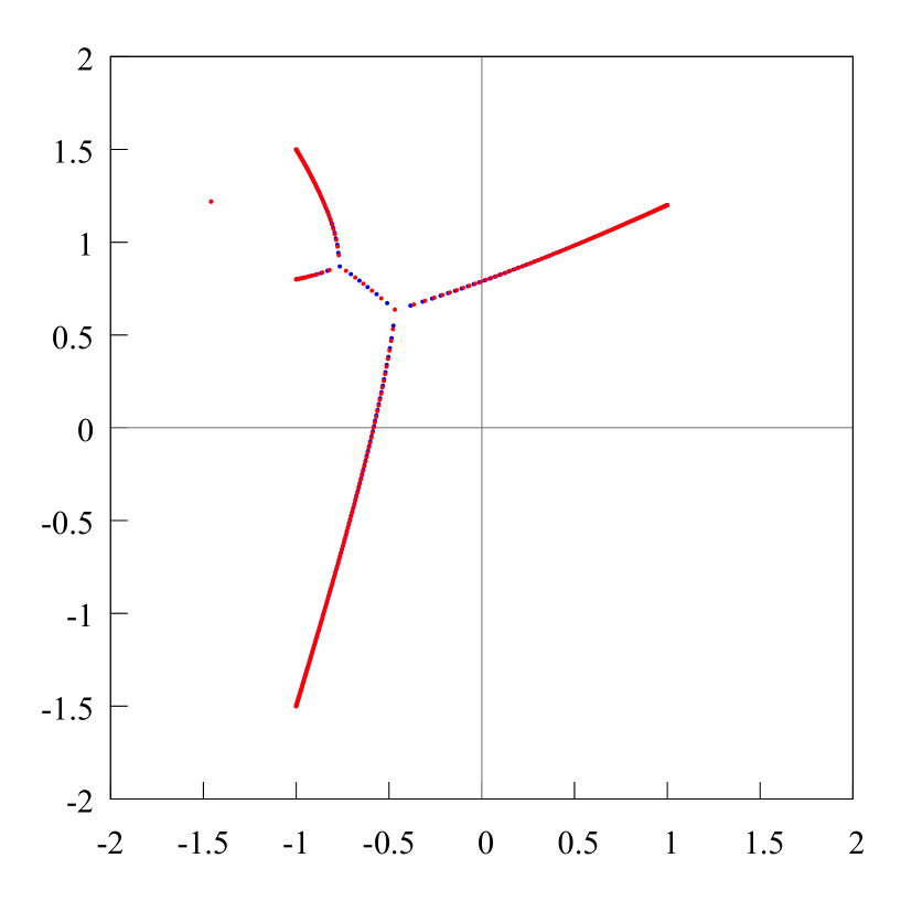
Figure 3. Zeros (blue points) and poles (red points) of PA $[300/300]_{f}$ of the quadratic function $f(z)=\left(\dfrac{z-(-1.0+0.8i)}{z-(1.0+1.2i)}\right)^{1/2}+\left(\dfrac{z-(-1.0+1.5i)}{z-(-1.0-1.5i)}\right)^{1/2}$. There are $2$ Chebotarëv points on the picture. Thus the genus of the Stahl’s hyperelliptic Riemann surface is $2$. Here we observe a single Froissart doublet located in the second quadrant. In full compliance with the Rakhmanov’s model [45], the Froissart doublet attracts to itself the Stahl’s $S$-compact set $S_{300}$; cf. Fig. 4.

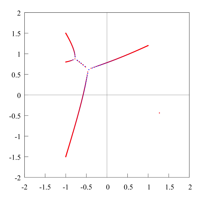
Figure 4. Zeros (blue points) and poles (red points) of PA $[300/300]_{f}$ of the logarithmic function $f(z)=\log\left(\dfrac{z-(-1.0+0.8i)}{z-(1.0+1.2i)}\right)+\log\left(\dfrac{z-(-1.0+1.5i)}{z-(-1.0-1.5i)}\right)$. There are $2$ Chebotarëv points on the picture. Thus the genus of the Stahl’s hyperelliptic Riemann surface is $2$. Here we observe a single Froissart doublet located in the fourth quadrant. In full compliance with the Rakhmanov’s model [45], the Froissart doublet attracts to itself the Stahl’s $S$-compact set $S_{300}$; cf. Fig. 3.

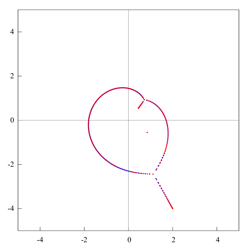
Figure 6. Numerical zeros (blue points) and poles (red points) distribution of two-point PA $[195/195]_{f}$ to the function $f(z)=\sqrt[4]{(z-a_{1})/(z-a_{2})}$, where $a_{1}=0.9-1.1i$ and $a_{2}=0.1+0.2i$. Here are selected two “quite different branches” of the function $f$, namely, $f_{0}=\sqrt[4]{(z-a_{1})/(z-a_{2})}$ and $f_{\infty}=-\sqrt[4]{(z-a_{1})/(z-a_{2})}$. All, but one pair, zeros (blue points) and poles (red points) approximate numerically Buslaev’s compact set. But there is a single Froissart doublet located in the domain $D_{0}(f)\ni 0$; cf. [58, Fig. 3].

References

- [1] A. I. Aptekarev, “Asymptotics of Hermite-Padé approximants for a pair of functions with branch points (Russian)”, Dokl. Akad. Nauk, 422:4 (2008), 443–445; translation in Dokl. Math., 78:2 (2008), 717–719.
- [2] A. I. Aptekarev, V. I. Buslaev, A. Martínez-Finkelshtein, S. P. Suetin, “Padé approximants, continued fractions, and orthogonal polynomials”, Russian Math. Surveys, 66:6 (2011), 1049–1131.
- [3] A. I. Aptekarev, A. Kuijlaars, “Hermite–Padé approximations and multiple orthogonal polynomial ensembles”, Russian Math. Surveys, 66:6 (2011), 1133–1199.
- [4] Alexander I. Aptekarev, Maxim L. Yattselev, “Padé approximants for functions with branch points – strong asymptotics of Nuttall–Stahl polynomials”, Acta Mathematica, 215: 2 (2015), 217–280.
- [5] N. U. Arakelian, “On efficient analytic continuation of power series” Math. USSR-Sb., 52:1 (1985), 21–39.
- [6] Baker, George A., Jr.; Graves-Morris, Peter, Padé approximants, Second edition, Encyclopedia of Mathematics and its Applications, 59, Cambridge University Press, Cambridge, 1996, xiv+746 pp. ISBN: 0-521-45007-1.
- [7] L. Baratchart, M. Yattselev, “Convergent interpolation to Cauchy integrals over analytic arcs”, Found. Comput. Math., 9 (2009), 675–715.
- [8] L. Bieberbach, Analytische Fortsetzung, Springer-Verlag, Berlin-Gottingen-Heidelberg, 1955, ii+168.
- [9] V. I. Buslaev, S. P. Suetin, “An extremal problem in potential theory”, Russian Math. Surveys, 69:5 (2014), 915–917.
- [10] V. I. Buslaev, A. Martínez-Finkelshtein, S. P. Suetin, “Method of interior variations and existence of -compact sets”, Proc. Steklov Inst. Math., 279 (2012), 25–51.
- [11] V. I. Buslaev, “Convergence of multipoint Padé approximants of piecewise analytic functions”, Sb. Math., 204:2 (2013), 190–222.
- [12] V. I. Buslaev, “Convergence of -point Padé approximants of a tuple of multivalued analytic functions”, Sb. Math., 206:2 (2015), 175–200.
- [13] V. I. Buslaev, “Capacity of a Compact Set in a Logarithmic Potential Field”, Proc. Steklov Inst. Math., 290 (2015), 238–255.
- [14] V. I. Buslaev, “An analogue of Polya’s theorem for piecewise holomorphic functions”, Sb. Math., 206:12 (2015), 1707–1721.
- [15] V. I. Buslaev, S. P. Suetin, “On Equilibrium Problems Related to the Distribution of Zeros of the Hermite–Padé Polynomials” Proc. Steklov Inst. Math., 290 (2015), 256–263.
- [16] P. Tchebycheff, “Sur les fractions continues”, J. de Math. Pures et Appl., Ser. 2, 3 (1858), 289–323.
- [17] Chudnovsky, D. V.; Chudnovsky, G. V., “The Wronskian formalism for linear differential equations and Padé approximations”, Adv. in Math., 53:1 (1984), 28–54.
- [18] Fidalgo Prieto U., Lopez Lagomasino G., “Nikishin Systems Are Perfect”, Constr. Approx., 34:3 (2011), 297–356.
- [19] M. Froissart, “Approximation de Padé: application a la physique des particules elementaires”, Recherche Cooperative sur Programme (RCP), 9, eds. Carmona, J., Froissart, M., Robinson, D.W., Ruelle, D., Centre National de la Recherche Scientifique (CNRS), Strasbourg, 1969, 1–13.
- [20] A. A. Gonchar, E. A. Rakhmanov, “On the convergence of simultaneous Padé approximants for systems of functions of Markov type”, Proc. Steklov Inst. Math., 157 (1983), 31–50.
- [21] A. A. Gonchar, E. A. Rakhmanov, “Equilibrium distributions and degree of rational approximation of analytic functions”, Math. USSR-Sb., 62:2 (1989), 305–348.
- [22] A. A. Gonchar, “Rational Approximations of Analytic Functions”, Proc. Steklov Inst. Math., 272, suppl. 2 (2011), S44–S57.
- [23] A. A. Gonchar, E. A. Rakhmanov, V. N. Sorokin, “Hermite–Padé approximants for systems of Markov-type functions”, Sb. Math., 188:5 (1997), 671–696.
- [24] M. Huttner, “Constructible sets of linear differential equations and effective rational approximations of polylogarithmic functions”, Israel J. Math., 153 (2006), 1–43.
- [25] R. K. Kovacheva, S. P. Suetin, “Distribution of zeros of the Hermite–Padé polynomials for a system of three functions, and the Nuttall condenser”, Proc. Steklov Inst. Math., 284 (2014), 168–191.
- [26] N. R. Ikonomov, R. K. Kovacheva, S. P. Suetin, Some numerical results on the behavior of zeros of the Hermite–Padé polynomials, 2015, 95 pp, arXiv:1501.07090.
- [27] N. R. Ikonomov, R. K. Kovacheva, S. P. Suetin, On the limit zero distribution of type I Hermite–Padé polynomials, 2015, 67 pp, arXiv:1506.08031.
- [28] N. R. Ikonomov, R. K. Kovacheva, S. P. Suetin, “Nuttall’s integral equation and Bernshtein’s asymptotic formula for a complex weight”, Izv. RAN. Ser. Mat., 79:6 (2015), 125–144.
- [29] A. V. Komlov, S. P. Suetin, “Strong asymptotics of two-point Padé approximants for power-like multivalued functions”, Dokl. Math., 89:2 (2014), 165–168.
- [30] Kuijlaars, Arno B. J.; Silva, Guilherme L. F., “-curves in polynomial external fields”, J. Approx. Theory, 191 (2015), 1–37.
- [31] G. V. Kuz’mina, “Moduli of families of curves and quadratic differentials”, Proc. Steklov Inst. Math., 139 (1982), 1–231.
- [32] E. N. Laguerre, “Sur la réduction en fractions continues d’une fraction qui satisfait à une équation différentiélle linéaire du premier ordre dont les coefficients sont rationnels”, J. de Math. Pures Appl., 1 (4) (1885), 135–165.
- [33] Landkof, N. S., Foundations of modern potential theory, Translated from the Russian by A. P. Doohovskoy, Die Grundlehren der mathematischen Wissenschaften, Band 180, Springer-Verlag, New York-Heidelberg,, 1972, x+424 pp.
- [34] M. A. Lapik, “Families of vector measures which are equilibrium measures in an external field”, Sb. Math., 206:2 (2015), 211–224.
- [35] G. Lopez Lagomasino, S. Medina Peralta, U. Fidalgo Prieto, “Hermite–Padé approximation for certain systems of meromorphic functions”, Sb. Math., 206:2 (2015), 225–241.
- [36] A. Martínez-Finkelshtein, E. A. Rakhmanov, S. P. Suetin, “Heine, Hilbert, Padé, Riemann, and Stieltjes: a John Nuttall’s work 25 years later”, Recent Advances in Orthogonal Polynomials, Special Functions, and Their Applications, 11th International Symposium (August 29-September 2, 2011 Universidad Carlos III de Madrid Leganes, Spain), Contemporary Mathematics, 578, eds. J. Arvesú, and G. López Lagomasino, American Mathematical Society, Providence, RI, 2012, 165–193.
- [37] A. Martínez-Finkelshtein, E. A. Rakhmanov, S. P. Suetin, “A differential equation for Hermite–Padé polynomials”, Russian Math. Surveys, 68:1 (2013), 183–185.
- [38] A. Martínez-Finkelshtein, E. A. Rakhmanov, S. P. Suetin, “Asymptotics of type I Hermite–Padé polynomials for semiclassical functions”, Contemporary Mathematics, 2015 (accepted).
- [39] E. M. Nikishin, “Asymptotic behavior of linear forms for simultaneous Padé approximants”, Soviet Math. (Iz. VUZ), 30:2 (1986), 43–52.
- [40] Nikishin, E. M.; Sorokin, V. N., Rational approximations and orthogonality, Translated from the Russian by Ralph P. Boas, Translations of Mathematical Monographs, 92, American Mathematical Society, Providence, RI, 1991, viii+221 pp. ISBN: 0-8218-4545-4.
- [41] J. Nuttall, “Asymptotics of diagonal Hermite–Padé polynomials”, J. Approx.Theory, 42 (1984), 299–386.
- [42] J. Nuttall, “Asymptotics of generalized Jacobi polynomials”, Constr. Approx., 2:1 (1986), 59–77.
- [43] J. Nuttall, “Padé polynomial asymptotics from a singular integral equation”, Constr. Approx., 6:2 (1990), 157–166.
- [44] O. Perron, Die Lehre von den Kettenbrüchen, Bd. II, Teubner, Stuttgart, 1957.
- [45] E. A. Rakhmanov, “Orthogonal polynomials and S-curves”, Recent Advances in Orthogonal Polynomials, Special Functions, and Their Applications, 11th International Symposium (August 29-September 2, 2011 Universidad Carlos III de Madrid Leganes, Spain), Contemporary Mathematics, 578, eds. J. Arvesú, and G. López Lagomasino, American Mathematical Society, Providence, RI, 2012, 195–239.
- [46] E. A. Rakhmanov, S. P. Suetin, “The distribution of the zeros of the Hermite-Padé polynomials for a pair of functions forming a Nikishin system”, Sb. Math., 204:9 (2013), 1347–1390.
- [47] E. A. Rakhmanov, “Gonchar-Stahl’s -theorem and associated directions in the theory of rational approximation of analytic functions”, Sb. Math., 2016, accepted, 30 pp.; arXiv:1503.06620.
- [48] E. B. Saff, V. Totik, Logarithmic potentials with external fields, Appendix B by Thomas Bloom, Grundlehren der Mathematischen Wissenschaften, 316, Springer-Verlag, Berlin, 1997.
- [49] H. Stahl, “Extremal domains associated with an analytic function. I”, Complex Variables Theory Appl., 4 (1985), 311–324.
- [50] H. Stahl, “Extremal domains associated with an analytic function. II”, Complex Variables Theory Appl., 4 (1985), 325–338.
- [51] H. Stahl, “Structure of extremal domains associated with an analytic function”, Complex Variables Theory Appl., 4 (1985), 339–354.
- [52] H. Stahl, “Orthogonal polynomials with complex valued weight function. I”, Constr. Approx., 2 (1986), 225–240.
- [53] H. Stahl, “Orthogonal polynomials with complex valued weight function. II”, Constr. Approx., 2 (1986), 241–251.
- [54] H. Stahl, “Asymptotics of Hermite–Padé polynomials and related convergence results. A summary of results”, Nonlinear numerical methods and rational approximation (Wilrijk, 1987), Math. Appl., 43, Reidel, Dordrecht, 1988, 23–53; also the fulltext preprint version is avaible, 79 pp.
- [55] H. Stahl, “The convergence of Padé approximants to functions with branch points”, J. Approx. Theory, 91:2 (1997), 139–204.
- [56] S. P. Suetin, “Uniform convergence of Padé diagonal approximants for hyperelliptic functions”, Sb. Math., 191:9 (2000), 81–114.
- [57] Sergey Suetin, On the distribution of zeros of the Hermite–Padé polynomials for three algebraic functions and the global topology of the Stokes lines for some differential equations of the third order, 2013, 59 pp, arXiv:1312.7105.
- [58] S. P. Suetin, “Distribution of the zeros of Padé polynomials and analytic continuation”, Russian Math. Surveys, 70:5 (2015), 901–951.
- [59] Gabor Szegö, Orthogonal polynomials, Fourth edition, Colloquium Publications, XXIII, American Mathematical Society, Providence, R.I., 1975, xiii+432 pp.