Analysis and Design of Phase Desynchronization in Pulse-coupled Oscillators

Abstract

By spreading phases on the unit circle, desynchronization algorithm is a powerful tool to achieve round-robin scheduling, which is crucial in applications as diverse as media access control of communication networks, realization of analog-to-digital converters, and scheduling of traffic flows in intersections. Driven by the increased application of pulse-coupled oscillators in achieving synchronization, desynchronization of pulse-coupled oscillators is also receiving more attention. In this paper, we propose a phase desynchronization algorithm by rigorously analyzing the dynamics of pulse-coupled oscillators and carefully designing the pulse based interaction function. A systematic proof for convergence to phase desynchronization is also given. Different from many existing results which can only achieve equal separation of firing time instants, the proposed approach can achieve equal separation of phases, which is more difficult to achieve due to phase jumps in pulse-coupled oscillators. Furthermore, the new strategy can guarantee achievement of desynchronization even when some nodes have identical initial phases, a situation which fails most existing desynchronization approaches. Numerical simulation results are provided to illustrate the effectiveness of the theoretical results.

I Introduction

Pulse-coupled oscillators (PCOs) were originally proposed to model synchronization in biological systems such as flashing fireflies [1, 2] and firing neurons [3, 4]. In recent years, with impressive scalability, simplicity, accuracy, and robustness, the PCO based synchronization strategy has become a powerful clock synchronization primitive for wireless sensor networks [5, 6, 7, 8, 9].

A less explored property of pulse-coupled oscillators is desynchronization, which spreads the phase variables of all PCOs uniformly apart (with equal difference between neighboring phases). Desynchronization has been found in many biological phenomena, such as spiking neuron networks [10] and the communication signals of fish [11]. What’s more, desynchronization is also very important for Deep Brain Stimulation (DBS) which has been proven an effective treatment for Parkinson’s disease [12]. Recently, phase desynchronization has also been employed to perform time-division multiple access (TDMA) medium access control (MAC) protocol [13, 14, 15]. Since desynchronization enables all agents to send messages in a round-robin manner, it provides collision-free message transmissions and obtains a high throughput [16].

In the literature, a number of papers have emerged on PCO based desynchronization. Based on the PCO model in [1], the authors in [17] proposed a desynchronization algorithm (INVERSE-MS) for an all-to-all network. The convergence property of INVERSE-MS was further explored in [18] and [19, 20], using an algebraic framework and a hybrid systems framework, respectively. However, all the above results are about the achievement of uniform firing time interval (equal time interval between any two consecutive PCOs’ firings), which is referred to as weak desynchronization [17], [18]. Weak desynchronization relies on persistent phase jumps to achieve equal time interval between consecutive firings, and hence cannot guarantee uniformly spread of phases.

Recently, algorithms also emerged for phase desynchronization. The authors in [21] proposed DESYNC in which each PCO relies on the firing information of the PCOs firing before and after this PCO when updating its phase variable. A modified algorithm V-DESYNC was proposed in [22] to mitigate the beacon collision problem by randomly adding a small offset to the firing time. The authors in [18, 23] proposed a phase desynchronization algorithm by limiting the listening interval. The authors in [24] obtained phase desynchronization by adding an anchored PCO that never adjusts its phase when other PCOs fire. Generally speaking, performance of these desynchronization algorithms is very difficult to analyze rigorously unless some kind of approximation is performed first to simplify the PCO dynamics. Recently, a stochastic framework is introduced to analyze the statistical behavior of the above desynchronization algorithms [25, 26, 27, 28]. However, such stochastic analysis assumes that PCO phase variables are subject to additive white noise, which is restrictive in many applications. In fact, as pointed out in [24], there is still a lack of rigorous mathematical proof for the convergence of PCO based phase desynchronization algorithms.

In this paper, we propose a distributed PCO based phase desynchronization algorithm, and systematically characterize its convergence properties using rigorously mathematical analysis. In addition, through designing the update rule we can achieve desynchronization even when some nodes have equal initial phase values, a situation which fails almost all existing PCO based desynchronization approaches.

II PCO based phase desynchronization

In this section, we will first introduce the PCO model, and then we propose a phase desynchronization algorithm.

II-A PCO model

We consider a network of $N$ PCOs with an all-to-all communication pattern. Each oscillator has a phase variable $\phi_{k}\in\mathbb{S}^{1}$ ($k=1,2,\ldots,N$) where $\mathbb{S}^{1}$ denotes the one-dimensional torus. Each phase variable $\phi_{k}$ evolves continuously from 0 to $2\pi$ with a constant speed determined by its natural frequency $w_{k}$. In this paper, the natural frequencies are assumed identical, i.e., $w_{1}=w_{2}=\ldots=w_{N}=w$. When an oscillator’s phase reaches $2\pi$, it fires (emit a pulse) and resets its phase to $0$, after which the cycle repeats. When an oscillator receives a pulse from a neighboring oscillator, it shifts its phase by a certain amount according to the phase response function, which is defined below:

Definition 1

Phase response function $F(\phi_{k})$ is defined as the phase shift (or jump) induced by a pulse as a function of phase at which the pulse is received [29].

Therefore, the interaction mechanism of PCOs can be described as follows:

1. Each PCO has a phase variable $\phi_{k}\in\mathbb{S}^{1}$ with initial value set to $\phi_{k}(0)$. $\phi_{k}$ evolves continuously from $0$ to $2\pi$ with a constant speed $w$;

2. When the phase variable $\phi_{k}$ of PCO $k$ reaches $2\pi$, this PCO fires, i.e., emits a pulse, and simultaneously resets $\phi_{k}$ to 0. Then the same process repeats;

3. When a PCO receives a pulse from others, it updates its phase variable according to the phase response function $F(\phi_{k})$:

   $$\phi_{k}^{+}=\phi_{k}+F(\phi_{k})$$ (1)

   where $\phi_{k}^{+}$ and $\phi_{k}$ denote the phases of the $k$th oscillator after and before a pulse.

II-B PCO based phase desynchronization

It is already well-known that if the phase response function is chosen appropriately, pulse-coupled oscillators can achieve synchronization. For example, reference [30] shows that using a delay-advance phase response function in which the value of phase shift is negative in the interval $(0,\pi)$, positive in the interval $(\pi,2\pi)$, and zero at $0$ and $2\pi$, oscillator phases can achieve synchronization.

Inspired by this idea, we propose a phase desynchronization algorithm by designing the phase response function of PCOs. Phase desynchronization in this paper is defined as follows:

Definition 2

For a network of $N$ oscillators, phase desynchronization denotes the state on which all phase are distributed evenly on the unit circle with identical differences $\frac{2\pi}{N}$ between any two adjacent phases.

As discussed earlier, in PCO networks, phase desynchronization is more stringent than weak desynchronization [17, 18] which uniformly spreads firing time instants of constituent nodes. This is because in PCO networks, weak desynchronization can be realized by using persistent phase jumps (caused by pulse interactions), which is not permitted by phase desynchronization; whereas weak synchronization follows naturally if phase desynchronization is achieved.

The phase response function $F(\phi_{k})$ we propose is given by

$$F(\phi_{k})=\left\{\begin{aligned} &-l(\phi_{k}-\frac{2\pi}{N})&{\quad}&0\leq\phi_{k}<\frac{2\pi}{N}\\ &\quad 0&{\quad}&\frac{2\pi}{N}\leq\phi_{k}\leq 2\pi\end{aligned}\right.$$ (2)

where $0<l<1$. According to this phase response function, PCO $k$ updates its phase variable $\phi_{k}$ only when $\phi_{k}$ is within the interval $[0,\frac{2\pi}{N})$ as illustrated in Fig. 1. Therefore, the phase update (1) can be rewritten as:

$$\phi_{k}^{+}=\left\{\begin{aligned} &(1-l)\phi_{k}+l\frac{2\pi}{N}&{\quad}&0\leq\phi_{k}<\frac{2\pi}{N}\\ &\quad\phi_{k}&{\quad}&\frac{2\pi}{N}\leq\phi_{k}\leq 2\pi\end{aligned}\right.$$ (3)

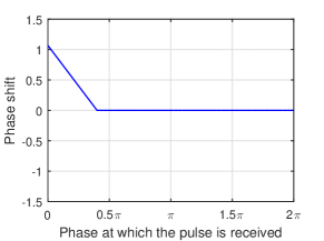
Figure 1: Phase response function (2) for phase desynchronization algorithm based on PCOs ($N=5$, $l=0.85$).

Theorem 1

For a network of $N$ PCOs with no two PCOs having identical initial phases, the PCOs will achieve phase desynchronization if the phase response function $F(\phi_{k})$ is given by (2) for $0<l<1$.

Intuitively, under the phase response function (2) which is positive in the interval $[0,\frac{2\pi}{N})$, an oscillator whose phase variable $\phi_{k}$ satisfies $\phi_{k}\in[0,\frac{2\pi}{N})$ will be pushed toward $\frac{2\pi}{N}$ when it receives a pulse from a firing oscillator (whose phase should be $2\pi$). Therefore, the phase difference between oscillator $k$ and the oscillator who just fired will evolve towards $\frac{2\pi}{N}$. In the next section, we will provide a rigorous mathematical proof for Theorem $1$.

III Convergence properties of the proposed phase desynchronization algorithm

In order to prove Theorem 1, we need Theorem 2 on the firing order of PCOs.

Theorem 2

Under the phase response function (2), the firing order of PCOs is time-invariant, i.e., if initially the $i$th oscillator fires immediately after the $j$th oscillator, then it will always fires immediately after the $j$th oscillator. In other words, the phase response function will not make one phase variable overpass another on $\mathbb{S}^{1}$.

Proof: Assume that a phase variable $\phi_{k}$ reaches $2\pi$ and emits a pulse at time instant $t_{k}$. Then after receiving this pulse, all the other phase variables will update their values according to (2). Suppose there are two phase variables satisfying $\phi_{i}<\phi_{j}$ before the pulse-induced update, and their values after update are denoted by $\phi_{i}^{+}$ and $\phi_{j}^{+}$, respectively. To prove theorem 2, we only need to show that $\phi_{i}^{+}<\phi_{j}^{+}$ is always true. Because the values of $\phi_{i}$ and $\phi_{j}$ are changed by pulses only when they are less than $\frac{2\pi}{N}$, depending on the relationship between $\phi_{i}$, $\phi_{j}$, and $\frac{2\pi}{N}$, we divide the analysis into the following three cases:

1. If $\phi_{i}\geq\frac{2\pi}{N}$ and $\phi_{j}\geq\frac{2\pi}{N}$ hold, then the values of both $\phi_{i}$ and $\phi_{j}$ will not be affected by the pulse according to (2). So it follows naturally that $\phi_{i}^{+}<\phi_{j}^{+}$ is still true after the pulse;

2. If $\phi_{i}<\frac{2\pi}{N}$ and $\phi_{j}<\frac{2\pi}{N}$ hold, then the values of both $\phi_{i}$ and $\phi_{j}$ will be changed by the pulse. According to the phase update (3), they will become

   $$\phi_{i}^{+}=(1-l)\phi_{i}+l\frac{2\pi}{N}$$ (4)

   and

   $$\phi_{j}^{+}=(1-l)\phi_{j}+l\frac{2\pi}{N}$$ (5)

   respectively. It can be verified that $\phi_{i}^{+}<\phi_{j}^{+}$ is still true if before the pulse the condition $\phi_{i}<\phi_{j}$ holds;

3. If $\phi_{i}<\frac{2\pi}{N}$ and $\phi_{j}\geq\frac{2\pi}{N}$ are true, then only the value of $\phi_{i}$ will be affected by the pulse. So we have $\phi_{j}^{+}=\phi_{j}\geq\frac{2\pi}{N}$ and $\phi_{i}^{+}=(1-l)\phi_{i}+l\frac{2\pi}{N}$, which is still less than $\frac{2\pi}{N}$ since

   $$\phi_{i}^{+}-\frac{2\pi}{N} =(1-l)\phi_{i}+l\frac{2\pi}{N}-\frac{2\pi}{N}$$ (6)

   $$=(\phi_{i}-\frac{2\pi}{N})(1-l)$$

   $$<0$$

   Therefore, we have $\phi_{i}^{+}<\frac{2\pi}{N}$ and $\phi_{j}^{+}\geq\frac{2\pi}{N}$, which means that $\phi_{i}^{+}<\phi_{j}^{+}$ is still true.

In conclusion, $\phi_{i}^{+}<\phi_{j}^{+}$ will always be true if $\phi_{i}<\phi_{j}$ holds, which means that the phase response function (2) will not change the firing order of all the PCOs. $\blacksquare$

To prove Theorem 1 we also need an index to measure the degree of achievement of desynchronization. Without loss of generality, we denote the initial time instant as $t=0$ and assume at $t=0$ that the phases of PCOs are arranged in a way such that $\phi_{1}(0)>\phi_{2}(0)>\ldots>\phi_{N}(0)$ holds, as illustrated in Fig. 2. (Note that here we assume that no two PCOs’ initial phases are identical. The assumption will be relaxed in Sec. IV.) From Theorem 2, we know that the firing order of PCOs will not be affected by the pulse-induced update. So if $\phi_{k}$ is the immediate follower (anti-clockwisely) of $\phi_{k-1}$ on $\mathbb{S}^{1}$ at $t=0$, it will always be the immediate follower (anti-clockwisely) of $\phi_{k-1}$ on $\mathbb{S}^{1}$. Therefore, the phase differences between neighboring PCOs can always be expressed as:

$$\left\{\begin{aligned} \Delta_{k}&=(\phi_{k}-\phi_{k+1})\ {\rm mod}\ 2\pi,\quad k=1,2,\ldots,N-1\\ \Delta_{N}&=(\phi_{N}-\phi_{1})\ {\rm mod}\ 2\pi\end{aligned}\right.$$ (7)

As we discussed earlier, phase desynchronization is defined as that the phase variables of all PCOs are uniformly spread apart. In other words, all the phase differences between neighboring (in terms of phase) PCOs are equal to $\frac{2\pi}{N}$. Therefore, for the convenience in analysis, we introduce an index $P$ to measure the degree of achievement of phase desynchronization by using the phase differences between neighboring (in terms of phase) PCOs:

$$P\triangleq\sum\limits_{k=1}^{N}|\Delta_{k}-\frac{2\pi}{N}|$$ (8)

When phase desynchronization is achieved, the phase differences between neighboring PCOs are equal to $\frac{2\pi}{N}$, so the index $P$ in (8) will reach its minimum $0$. It can also be easily verified that $P$ equals $0$ only when phase desynchronization is achieved.

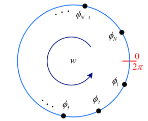
Figure 2: Initially (at $t=0$), the phases of PCOs are arranged in a way such that $\phi_{1}(0)>\phi_{2}(0)>\ldots>\phi_{N}(0)$ holds.

Therefore, in order to prove Theorem 1, we only need to prove that the index $P$ will converge to $0$ under the phase response function (2).

Proof of Theorem 1: From the analysis above, to prove Theorem 1, we only need to prove that the index $P$ will converge to $0$. According to the interaction mechanism of PCOs in Sec. II-A, all phase variables will evolve towards $2\pi$ with the same speed $w$, thus the phase differences between neighboring PCOs will not change during two consecutive pulses, neither will $P$. Therefore we only need to concentrate on how $P$ evolves at discrete-time instants when pulses are emitted.

After $t=0$, according to the dynamics of PCOs, all phase variables evolve towards $2\pi$ with the same speed $w$. Since $\phi_{1}$ is the largest, it will reach $2\pi$ first without perturbation (denote this time instant as $t=t_{1}$), upon which PCO $1$ will send a pulse which will be received by all the other PCOs. After receiving the pulse, PCO $i$ will update $\phi_{i}$ ($2\leq i\leq N$) according to (2). From (2), we know that the value of $\phi_{i}$ will be changed if it is within the interval $[0,\frac{2\pi}{N})$; otherwise, it will keep unchanged. Therefore we call the interval $[0,\frac{2\pi}{N})$ as the “effective interval.” If at least one phase variable is within the “effective interval,” then this phase variable will be affected by the pulse, which will in turn affect the phase differences between neighboring (in terms of phase) PCOs. In this case the pulse will be called an “active pulse.” Otherwise, if no $\phi_{i}$ ($2\leq i\leq N$) are within the “effective interval,” then the pulse from PCO $1$ will not affect any phase variable and it will be referred to as a “silent pulse.” If the pulse from PCO $1$ is a “silent pulse,” other than resetting $\phi_{1}$ from $2\pi$ to $0$, it will not disturb the evolution of any other phase variable towards $2\pi$. After $t=t_{1}$, $\phi_{1}$ becomes the smallest and $\phi_{2}$ becomes the largest who will reach $2\pi$ next. Suppose $\phi_{2}$ reaches $2\pi$ at time instant $t=t_{2}$ and emits a pulse. Similar to the pulse from PCO $1$, this pulse could be an “active pulse” or a “silent pulse.” Following the same line of reasoning, it can be inferred that $\phi_{3}$ will reach $2\pi$ after $\phi_{2}$’s resetting and its pulse can be an “active pulse” or a “silent pulse.” So do the other $\phi_{i}$s and their corresponding pulses. Next we prove that there cannot be $N$ consecutive “silent pulses” unless phase desynchronization is achieved.

We use proof of contradiction. Assume that $N$ consecutive pulses are all “silent pulses” but phase desynchronization has not been achieved. From Theorem 2, no phase variable can surpass another on $\mathbb{S}^{1}$, so the $N$ consecutive pulses must be from $N$ different PCOs. For a pulse from oscillator $i$ to be a “silent pulse,” the phase variable of the PCO who sents a pulse immediately before oscillator $i$ (whose phase is the smallest according to Theorem 2) must be no less than $\frac{2\pi}{N}$ (outside the “effective interval”). Therefore, if there are $N$ consecutive “silent pulses,” then the phase difference between any two neighboring PCOs is no less than $\frac{2\pi}{N}$. Because the sum of all the phase differences are $2\pi$, we can infer that all the phase differences are equal to $\frac{2\pi}{N}$, meaning that phase desynchronization is achieved, which contradicts the initial assumption.

Therefore, there cannot be $N$ consecutive “silent pulses” unless phase desynchronization is achieved. Without loss of generality, we assume that the pulse from oscillator $k$ is the first “active pulse,” and its phase variable $\phi_{k}$ reaches $2\pi$ at time instant $t=t_{k}$. Since the pulse is an “active pulse,” there is at least one phase variable within the “effective interval” when the pulse is sent. Without loss of generality, we assume that there are $M$ ($M$ is an integer satisfying $1\leq M\leq N-1$) phase variables within the “effective interval” which can be represented as $\phi_{\Widehat{k-1}},\ldots,\phi_{\Widehat{k-M}}$, where the superscript “ $\Widehat{}$ ” represents modulo operation on $N$, i.e., $\Widehat{\bullet}\triangleq(\bullet)\ {\rm mod}\ N$, as illustrated in Fig. 3. According to the assumption, we have $\phi_{\Widehat{k-M}}<\frac{2\pi}{N}\leq\phi_{\Widehat{k-M-1}}$. Since $\phi_{\Widehat{k-1}},\ldots,\phi_{\Widehat{k-M}}$ are in the “effective interval,” they will update their values after receiving the pulse from oscillator $k$ according to the phase update in (3) as follows:

$$\phi_{\Widehat{k-i}}^{+}=(1-l)\phi_{\Widehat{k-i}}+l\frac{2\pi}{N},\quad i=1,\ldots,M$$ (9)

Note that we also have $\phi_{k}^{+}=0$ and $\phi_{\Widehat{k-j}}^{+}=\phi_{\Widehat{k-j}}$ for $j=M+1,\ldots,N-1$ (because $\phi_{\Widehat{k-j}}$ for $j=M+1,\ldots,N-1$ are not in the “effective interval” and thus will not be changed according to the phase response function in (2)).

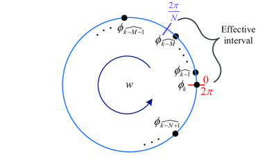
Figure 3: The phase variables $\phi_{\Widehat{k-1}},\ldots,\phi_{\Widehat{k-M}}$ are in the “effective interval” when oscillator $k$ sends the first “active pulse” at $t=t_{k}$.

Therefore, phase differences after the update can be rewritten as follows:

$$\left\{\begin{aligned} &\Delta_{k}^{+}=\phi_{k}^{+}-\phi_{\Widehat{k-N+1}}^{+}+2\pi=2\pi-\phi_{\Widehat{k-N+1}}\\ &\Delta_{\Widehat{k-1}}^{+}=\phi_{\Widehat{k-1}}^{+}-\phi_{k}^{+}=(1-l)\phi_{\Widehat{k-1}}+l\frac{2\pi}{N}\\ &\Delta_{\Widehat{k-i}}^{+}=\phi_{\Widehat{k-i}}^{+}-\phi_{\Widehat{k-i+1}}^{+}=(1-l)(\phi_{\Widehat{k-i}}-\phi_{\Widehat{k-i+1}}),i=2,\ldots,M\\ &\Delta_{\Widehat{k-M-1}}^{+}=\phi_{\Widehat{k-M-1}}^{+}-\phi_{\Widehat{k-M}}^{+}=\phi_{\Widehat{k-M-1}}-(1-l)\phi_{\Widehat{k-M}}-l\frac{2\pi}{N}\\ &\Delta_{\Widehat{k-j}}^{+}=\phi_{\Widehat{k-j}}^{+}-\phi_{\Widehat{k-j+1}}^{+}=\phi_{\Widehat{k-j}}-\phi_{\Widehat{k-j+1}},j=M+2,\ldots,N-1\\ \end{aligned}\right.$$ (10)

According to (8), the new $P$ (denote it as $P^{+}$) after the update is given by:

$$P^{+}=\sum\limits_{j=0}^{N-1}|\Delta_{\Widehat{k-j}}^{+}-\frac{2\pi}{N}|$$ (11)

To show that the pulse from oscillator $k$ will decrease $P$, we calculate the difference of $P$ before and after the pulse-induced update:

$$P^{+}-P =\sum\limits_{j=0}^{N-1}|\Delta_{\Widehat{k-j}}^{+}-\frac{2\pi}{N}|-\sum\limits_{j=0}^{N-1}|\Delta_{\Widehat{k-j}}-\frac{2\pi}{N}|$$ (12)

$$=\underbrace{|\Delta_{k}^{+}-\frac{2\pi}{N}|-|\Delta_{k}-\frac{2\pi}{N}|}_{\rm part\,1}+\underbrace{|\Delta_{\Widehat{k-1}}^{+}-\frac{2\pi}{N}|-|\Delta_{\Widehat{k-1}}-\frac{2\pi}{N}|}_{\rm part\,2}$$

$$\quad+\underbrace{\sum\limits_{i=2}^{M}|\Delta_{\Widehat{k-i}}^{+}-\frac{2\pi}{N}|-\sum\limits_{i=2}^{M}|\Delta_{\Widehat{k-i}}-\frac{2\pi}{N}|}_{\rm part\,3}$$

$$\quad+\underbrace{|\Delta_{\Widehat{k-M-1}}^{+}-\frac{2\pi}{N}|-|\Delta_{\Widehat{k-M-1}}-\frac{2\pi}{N}|}_{\rm part\,4}$$

$$\quad+\underbrace{\sum\limits_{j=M+2}^{N-1}|\Delta_{\Widehat{k-j}}^{+}-\frac{2\pi}{N}|-\sum\limits_{j=M+2}^{N-1}|\Delta_{\Widehat{k-j}}-\frac{2\pi}{N}|}_{\rm part\,5}$$

The part 1, part 2, part 3, and part 5 in (12) can be simplified as follows, respectively:

1. $$\underbrace{|\Delta_{k}^{+}-\frac{2\pi}{N}|-|\Delta_{k}-\frac{2\pi}{N}|}_{\rm part\,1}$$ (13)

   $$= |2\pi-\phi_{\Widehat{k-N+1}}-\frac{2\pi}{N}|-|2\pi-\phi_{\Widehat{k-N+1}}-\frac{2\pi}{N}|$$

   $$= \ 0$$

2. $$\underbrace{|\Delta_{\Widehat{k-1}}^{+}-\frac{2\pi}{N}|-|\Delta_{\Widehat{k-1}}-\frac{2\pi}{N}|}_{\rm part\,2}$$ (14)

   $$= |(1-l)\phi_{\Widehat{k-1}}+l\frac{2\pi}{N}-\frac{2\pi}{N}|-|\phi_{\Widehat{k-1}}-\frac{2\pi}{N}|$$

   $$= (1-l)(\frac{2\pi}{N}-\phi_{\Widehat{k-1}})-(\frac{2\pi}{N}-\phi_{\Widehat{k-1}})$$

   $$= -l(\frac{2\pi}{N}-\phi_{\Widehat{k-1}})$$

   In the above derivation we used $\phi_{\Widehat{k-1}}<\frac{2\pi}{N}$.

3. $$\underbrace{\sum\limits_{i=2}^{M}|\Delta_{\Widehat{k-i}}^{+}-\frac{2\pi}{N}|-\sum\limits_{i=2}^{M}|\Delta_{\Widehat{k-i}}-\frac{2\pi}{N}|}_{\rm part\,3}$$ (15)

   $$= \sum\limits_{i=2}^{M}\{|(1-l)(\phi_{\Widehat{k-i}}-\phi_{\Widehat{k-i+1}})-\frac{2\pi}{N}|$$

   $$\quad-|(\phi_{\Widehat{k-i}}-\phi_{\Widehat{k-i+1}})-\frac{2\pi}{N}|\}$$

   $$= \sum\limits_{i=2}^{M}\{\frac{2\pi}{N}-(1-l)(\phi_{\Widehat{k-i}}-\phi_{\Widehat{k-i+1}})-\frac{2\pi}{N}$$

   $$\quad+(\phi_{\Widehat{k-i}}-\phi_{\Widehat{k-i+1}})\}$$

   $$= \sum\limits_{i=2}^{M}l(\phi_{\Widehat{k-i}}-\phi_{\Widehat{k-i+1}})$$

   where we used the relationships $\phi_{\Widehat{k-i}}-\phi_{\Widehat{k-i+1}}<\frac{2\pi}{N}$ and $(1-l)(\phi_{\Widehat{k-i}}-\phi_{\Widehat{k-i+1}})<\frac{2\pi}{N}$, $i=2,\ldots,M$.

4. $$\underbrace{\sum\limits_{j=M+2}^{N-1}|\Delta_{\Widehat{k-j}}^{+}-\frac{2\pi}{N}|-\sum\limits_{j=M+2}^{N-1}|\Delta_{\Widehat{k-j}}-\frac{2\pi}{N}|}_{\rm part\,5}$$ (16)

   $$= \sum\limits_{j=M+2}^{N-1}\{|\phi_{\Widehat{k-j}}-\phi_{\Widehat{k-j+1}}-\frac{2\pi}{N}|-|\phi_{\Widehat{k-j}}-\phi_{\Widehat{k-j+1}}-\frac{2\pi}{N}|\}$$

   $$= \ 0$$

Combining (12)-(16) leads to:

$$P^{+}-P= -l(\frac{2\pi}{N}-\phi_{\Widehat{k-1}})+\sum\limits_{i=2}^{M}l(\phi_{\Widehat{k-i}}-\phi_{\Widehat{k-i+1}})$$ (17)

$$\quad+|\Delta_{\Widehat{k-M-1}}^{+}-\frac{2\pi}{N}|-|\Delta_{\Widehat{k-M-1}}-\frac{2\pi}{N}|$$

$$= l\phi_{\Widehat{k-M}}-l\frac{2\pi}{N}+|\Delta_{\Widehat{k-M-1}}^{+}-\frac{2\pi}{N}|-|\Delta_{\Widehat{k-M-1}}-\frac{2\pi}{N}|$$

Next, we discuss the value of $P^{+}-P$ in (17) under three different cases:

1. If $\Delta_{\Widehat{k-M-1}}>\frac{2\pi}{N}$ and $\Delta_{\Widehat{k-M-1}}^{+}\geq\frac{2\pi}{N}$ hold, (17) can be rewritten as:

   $$P^{+}-P= l\phi_{\Widehat{k-M}}-l\frac{2\pi}{N}+\Delta_{\Widehat{k-M-1}}^{+}-\Delta_{\Widehat{k-M-1}}$$ (18)

   $$= l\phi_{\Widehat{k-M}}-l\frac{2\pi}{N}+\phi_{\Widehat{k-M-1}}-(1-l)\phi_{\Widehat{k-M}}$$

   $$\quad-l\frac{2\pi}{N}-\phi_{\Widehat{k-M-1}}+\phi_{\Widehat{k-M}}$$

   $$= 2l(\phi_{\Widehat{k-M}}-\frac{2\pi}{N})$$

   $$< 0$$

2. If $\Delta_{\Widehat{k-M-1}}>\frac{2\pi}{N}$ and $\Delta_{\Widehat{k-M-1}}^{+}<\frac{2\pi}{N}$ hold, we have $\phi_{\Widehat{k-M}}-\phi_{\Widehat{k-M-1}}+\frac{2\pi}{N}<0$. Then (17) can be rewritten as:

   $$P^{+}-P= l\phi_{\Widehat{k-M}}-l\frac{2\pi}{N}+\frac{2\pi}{N}-\Delta_{\Widehat{k-M-1}}^{+}-\Delta_{\Widehat{k-M-1}}$$ (19)

   $$\quad+\frac{2\pi}{N}$$

   $$= l\phi_{\Widehat{k-M}}-l\frac{2\pi}{N}+\frac{2\pi}{N}-\phi_{\Widehat{k-M-1}}+(1-l)\phi_{\Widehat{k-M}}$$

   $$\quad+l\frac{2\pi}{N}-\phi_{\Widehat{k-M-1}}+\phi_{\Widehat{k-M}}+\frac{2\pi}{N}$$

   $$= 2(\phi_{\Widehat{k-M}}-\phi_{\Widehat{k-M-1}}+\frac{2\pi}{N})$$

   $$< 0$$

3. If $\Delta_{\Widehat{k-M-1}}\leq\frac{2\pi}{N}$ and $\Delta_{\Widehat{k-M-1}}^{+}<\frac{2\pi}{N}$ hold, (17) can be rewritten as:

   $$P^{+}-P= l\phi_{\Widehat{k-M}}-l\frac{2\pi}{N}-\Delta_{\Widehat{k-M-1}}^{+}+\Delta_{\Widehat{k-M-1}}$$ (20)

   $$= l\phi_{\Widehat{k-M}}-l\frac{2\pi}{N}-\phi_{\Widehat{k-M-1}}+(1-l)\phi_{\Widehat{k-M}}$$

   $$\quad+l\frac{2\pi}{N}+\phi_{\Widehat{k-M-1}}-\phi_{\Widehat{k-M}}$$

   $$= 0$$

Remark 1

According to (2), we cannot have a fourth case where $\Delta_{\Widehat{k-M-1}}\leq\frac{2\pi}{N}$ and $\Delta_{\Widehat{k-M-1}}^{+}\geq\frac{2\pi}{N}$ hold because of the following constraint according to (7) and (10):

$$\Delta_{\Widehat{k-M-1}}^{+}-\Delta_{\Widehat{k-M-1}}$$ (21)

$$= \phi_{\Widehat{k-M-1}}-(1-l)\phi_{\Widehat{k-M}}-l\frac{2\pi}{N}-\phi_{\Widehat{k-M-1}}+\phi_{\Widehat{k-M}}$$

$$= l(\phi_{\Widehat{k-M}}-\frac{2\pi}{N})$$

$$< 0$$

It is worth noting that in (21) we used the initial assumption $\phi_{\Widehat{k-M}}<\frac{2\pi}{N}$.

From the above analysis, we know that the value of $P$ will be decreased or unchanged by each “active pulse.” Next we proceed to show that $P$ will not be retained at a non-zero value, i.e., the “Case 3” above cannot always be true before phase desynchronization is achieved.

It can be easily inferred that before achieving the phase desynchronization there always exists one phase difference larger than $\frac{2\pi}{N}$ and one phase difference smaller than $\frac{2\pi}{N}$, and in between the two phase differences there may be some phase differences (represent the number as $Q$, $0\leq Q\leq N-2$) that are equal to $\frac{2\pi}{N}$, which is defined as “state one.” Denote the phase difference larger than $\frac{2\pi}{N}$ and the phase difference smaller than $\frac{2\pi}{N}$ as $\Delta_{\Widehat{j-Q-2}}$ and $\Delta_{\Widehat{j-1}}$, respectively, and the $Q$ phase differences (which are equal to $\frac{2\pi}{N}$) in between as $\Delta_{\Widehat{j-2}},\ldots,\Delta_{\Widehat{j-Q-1}}$ (cf. Fig. 4). It can be proven that “state one” must evolve to a “state two” (cf. Fig. 5) after $Q(N-1)$ pulses. In the “state two,” the $Q$ phase differences which were equal to $\frac{2\pi}{N}$ in the “state one” become smaller than $\frac{2\pi}{N}$, meaning that the condition in “Case 3” is not satisfied when oscillator $\Widehat{j-Q}$ fires because phase $\phi_{\Widehat{j-Q-1}}$ is within the “effective interval” and $\Delta_{\Widehat{k-M-1}}=\Delta_{\Widehat{j-Q-2}}>\frac{2\pi}{N}$ ($k=\Widehat{j-Q}$ and $M=1$) is true.

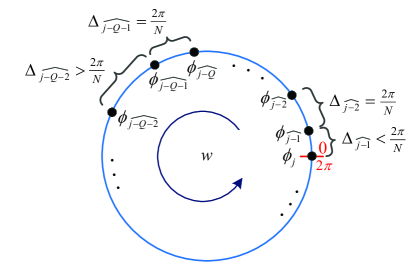
Figure 4: The “state one” that $Q$ ($0\leq Q\leq N-2$) phase differences between the larger phase difference and the smaller phase difference are equal to $\frac{2\pi}{N}$ .

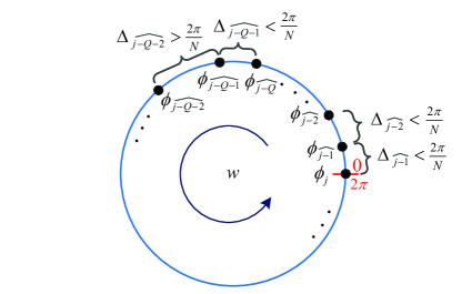
Figure 5: The “state two” that $Q$ ($0\leq Q\leq N-2$) phase differences between the larger phase difference and the smaller phase difference become smaller than $\frac{2\pi}{N}$.

Now we will illustrate how those phase differences equal to $\frac{2\pi}{N}$ become smaller than $\frac{2\pi}{N}$ after $Q(N-1)$ firing. Suppose at $t=t_{j}$, an “active pulse” is emitted by oscillator $j$. This pulse only affects $\phi_{\Widehat{j-1}}$ since only $\phi_{\Widehat{j-1}}$ is within the “effective interval,” and it increases the value of $\phi_{\Widehat{j-1}}$ ($\phi_{\Widehat{j-1}}^{+}-\phi_{\Widehat{j-1}}=l(\frac{2\pi}{N}-\phi_{\Widehat{j-1}})>0$), which in turn makes $\Delta_{\Widehat{j-2}}$ smaller than $\frac{2\pi}{N}$. As time evolves, oscillators $\Widehat{j+1},\ldots,\Widehat{j-Q-2}$ will fire one by one. To discuss the evolution of PCOs under these pulses, we need to distinguish between two different cases. The first case is that $\phi_{\Widehat{j-1}}$ is still within the “effective interval” which means that the pulses will make $\Delta_{\Widehat{j-2}}$ smaller and smaller. The second case is that $\phi_{\Widehat{j-1}}$ is not within the “effective interval” and thus it is not affected by those pulses. Therefore, $\Delta_{\Widehat{j-2}}$ keeps unchanged and is still smaller than $\frac{2\pi}{N}$ as we discussed above. Both cases render the same result that $\Delta_{\Widehat{j-2}}$ is smaller than $\frac{2\pi}{N}$ after those pulses. Next oscillators $\Widehat{j-Q-1},\ldots,\Widehat{j-2}$ will fire one after another. However, their pulses are all “silent pulses” since no phase variables are within the “effective interval.” So all the phase differences will keep unchanged, meaning that $\Delta_{\Widehat{j-Q-2}}$ is still larger than $\frac{2\pi}{N}$, $\Delta_{\Widehat{j-Q-1}},\ldots,\Delta_{\Widehat{j-3}}$ are equal to $\frac{2\pi}{N}$, and $\Delta_{\Widehat{j-2}}$ is smaller than $\frac{2\pi}{N}$. Therefore, after $N-1$ consecutive firing, the number of phase differences equal to $\frac{2\pi}{N}$ is reduced by one to $Q-1$, as illustrated in Fig. (6). Therefore, after $Q(N-1)$ firing, the phase differences equal to $\frac{2\pi}{N}$ in the “state one” become smaller than $\frac{2\pi}{N}$, which means that the “state two” is achieved.

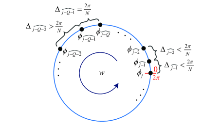
Figure 6: $Q-1$ ($0\leq Q\leq N-2$) phase differences between the larger phase difference and the smaller phase difference are equal to $\frac{2\pi}{N}$.

So the “state one” must evolve to the “state two,” and thus the condition in “Case 3” cannot always exist before achieving phase desynchronization because $\Delta_{\Widehat{k-M-1}}>\frac{2\pi}{N}$ ($k=\Widehat{j-Q}$ and $M=1$) will be true when PCO $\Widehat{j-Q}$ fires after the “state two” is achieved. Consequently, $P$ will keep decreasing until it reaches $0$, i.e., until phase desynchronization is achieved. Therefore, the PCOs will achieve phase desynchronization under the phase response function (2) for $0<l<1$. $\blacksquare$

IV Dealing with oscillators with identical phases

In Sec. II and Sec. III, we achieved phase desynchronization for a network of $N$ PCOs if no two oscillators have identical initial phases. In fact, under the proposed mechanism, if there are some oscillators (represent the number as $X$, $2\leq X\leq N$) having equal initial phases, these $X$ PCOs will always have equal phases. This is because these $X$ PCOs will always make updates simultaneously with identical phase shifts. Therefore, these $X$ PCOs will become inseparable, making phase desynchronization impossible.

We propose the following modifications to the original phase update rule to address this issue: When an oscillator’s phase reaches $2\pi$, this oscillator resets its phase to different values depending on whether a phase is detected. More specifically, if at this time instant, the oscillator also detect a pulse from its neighbor (meaning that this oscillator has equal phase with the neighbor), it will reset its phase to a value randomly chosen from $[0,2\pi)$; otherwise it will still reset its phase to 0.

Therefore, the interaction mechanism of PCOs will become:

1. Each PCO has a phase variable $\phi_{k}\in\mathbb{S}^{1}$ with initial value set to $\phi_{k}(0)$. $\phi_{k}$ evolves continuously from $0$ to $2\pi$ with a constant speed $w$;

2. When the phase variable $\phi_{k}$ of PCO $k$ reaches $2\pi$, this PCO fires, i.e., emits a pulse, and simultaneously resets $\phi_{k}$ to $\phi_{k,0}$ whose value depends on whether a pulse from a neighbor is detected: 1) if no pulses from neighbors are detected, then $\phi_{k,0}=0$; and 2) if a pulse from neighbors is detected, then $\phi_{k,0}$ will be a value randomly chosen from the interval $[0,\,2\pi)$. Then the same process repeats;

3. When a PCO receives a pulse from others, it updates its phase variable according to the phase response function $F(\phi_{k})$:

   $$\phi_{k}^{+}=\phi_{k}+F(\phi_{k})$$ (22)

   where $\phi_{k}^{+}$ and $\phi_{k}$ denote the phases of the $k$th oscillator after and before the pulse.

Under this new mechanism, oscillators with identical phases will be separated and hence desynchronization can also be achieved even some oscillator have equal initial phase values, which will be confirmed by numerical simulations in Sec. V.

V Simulation results

We use simulation results to demonstrate the proposed phase desynchronization algorithm. We first considered the case where no two oscillators have equal initial phases. The initial phases were randomly chosen from $[0,2\pi)$ and $l$ in the phase response function $(\ref{eqn:PRC})$ was set to $0.85$. $w$ was set to $2\pi$. The evolutions of oscillator phases, phase differences between neighboring PCOs, and the index $P$ are given in Fig. 7 and Fig. 8, respectively. It can be seen that the PCO phases were uniformly spread apart, the phase differences between neighboring PCOs converged to $\frac{2\pi}{5}$, and the index $P$ converges to $0$. This confirmed the effectiveness of the proposed desynchronization algorithm.

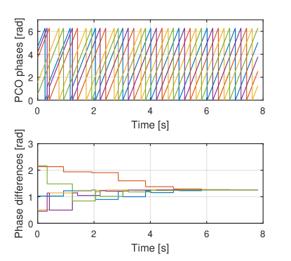
Figure 7: The evolution of PCO phases $\phi_{k}(k=1,\ldots,N)$ (upper panel) and phase differences between neighboring PCOs $\Delta_{k}(k=1,\ldots,N)$ (lower panel) under the phase response function $(\ref{eqn:PRC})$. The initial phase values were randomly chosen from the interval $[0,\,2\pi)$.

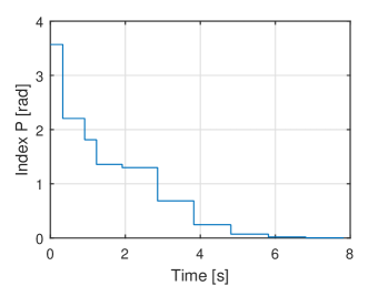
Figure 8: The evolution of index $P$ under the phase response function $(\ref{eqn:PRC})$. The initial phase values were randomly chosen from the interval $[0,\,2\pi)$.

We also considered the case where oscillators may have equal initial phases. We set the initial phases of all oscillators to $\pi$ and set $l$ in $(\ref{eqn:PRC})$ to $0.85$. $w$ was set to $2\pi$. Under the mechanism in Sec. IV, the evolutions of oscillator phases, phase differences between neighboring oscillators, and the index $P$ are given in Fig. 9 and Fig. 10, respectively. It can be seen that the proposed phase desynchronization approach can indeed achieve phase desynchronization even when all PCOs have equal initial phases.

Figure 9: The evolution of oscillator phases $\phi_{k}(k=1,\ldots,N)$ (upper panel) and phase differences between neighboring oscillators $\Delta_{k}(k=1,\ldots,N)$ (lower panel) under the phase response function $(\ref{eqn:PRC})$. The initial phases of all nodes were set to the same value.

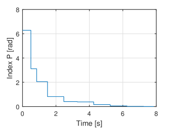
Figure 10: The evolution of the index $P$ under the phase response function $(\ref{eqn:PRC})$. The initial phases of all nodes were set to the same value.

VI Conclusions

A phase desynchronization approach is proposed based on the pulse coupled oscillators. Different from existing results which address equal separation of firing time instants and thus are subject to uneven spread of phases due to pulse based interaction, the proposed approach can achieve constant and even phase spread and its performance is guaranteed by systematic and rigorously mathematical analysis. Further more, we also proposed a mechanism to achieve desynchronization when some oscillators have equal initial phases, under which condition almost all existing approaches fail to fulfil desynchroniztion. Numerical simulations are given to confirm the theoretical results.

References

- [1] R. Mirollo and S. Strogatz. Synchronization of pulse-coupled biological oscillators. SIAM J. Appl. Math., 50:1645–1662, 1990.
- [2] P. Goel and B. Ermentrout. Synchrony, stability, and firing patterns in pulse-coupled oscillators. Physica D: Nonlinear Phenomena, 163(3):191–216, 2002.
- [3] C. S. Peskin. Mathematical aspects of heart physiology. Courant Institute of Mathematical Science, New York University, New York, 1975.
- [4] B. Ermentrout. Type I membrances, phase resetting curves, and synchrony. Neural Comput., 8(5):979–1001, 1996.
- [5] O. Simeone, U. Spagnolini, Y. Bar-Ness, and S Strogatz. Distributed synchronization in wireless networks. IEEE Signal Process. Mag., 25:81–97, 2008.
- [6] A. Tyrrell, G. Auer, and C. Bettstetter. Emergent slot synchronization in wireless networks. IEEE. Trans. Mob. Comput., 9:719–732, 2010.
- [7] G. Werner-Allen, G. Tewari, A. Patel, M. Welsh, and R. Nagpal. Firefly inspired sensor network synchronicity with realistic radio effects. In Proc. SenSys 05, pages 142 –153, USA, 2005.
- [8] Y. Q. Wang, F. Núez, and F. J. Doyle III. Increasing sync rate of pulse-coupled oscillators via phase response function design: theory and application to wireless networks. IEEE Trans. Control Syst. Technol., 21:1455–1462, 2013.
- [9] Y. Q. Wang, F. Nunez, and F. Doyle. Energy-efficient pulse-coupled synchronization strategy design for wireless sensor networks through reduced idle listening. IEEE Trans. Signal Process., 60(10):5293–5306, 2012.
- [10] M. Stopfer, S. Bhagavan, B. H. Smith, and G. Laurent. Impaired odour discrimination on desynchronization of odour-encoding neural assemblies. Nature, 390(6655):70–74, 1997.
- [11] J. Benda, A. Longtin, and L. Maler. A synchronization-desynchronization code for natural communication signals. Neuron, 52(2):347–358, 2006.
- [12] A. Nabi and J. Moehlis. Nonlinear hybrid control of phase models for coupled oscillators. In American Control Conference (ACC), 2010, pages 922–923, Baltimore, USA, 2010. IEEE.
- [13] J. Degesys, I. Rose, A. Patel, and R. Nagpal. DESYNC: self-organizing desynchronization and TDMA on wireless sensor networks. In Proc. IPSN 07, pages 11–20, Massachusetts, USA, 2007.
- [14] S. Ashkiani and A. Scaglione. Pulse coupled discrete oscillators dynamics for network scheduling. In Communication, Control, and Computing (Allerton), 2012 50th Annual Allerton Conference on, pages 1551–1558, UIUC, USA, 2012. IEEE.
- [15] Y. Taniguchi, G. Hasegawa, and H. Nakano. Self-organizing transmission scheduling considering collision avoidance for data gathering in wireless sensor networks. Journal of Communications, 8(6), 2013.
- [16] J. Degesys, I. Rose, A. Patel, and R. Nagpal. Self-organizing desynchronization and tdma on wireless sensor networks. In Bio-Inspired Computing and Communication, pages 192–203. Springer, 2008.
- [17] A. Patel, J. Degesys, and R. Nagpal. Desynchronization: The theory of self-organizing algorithms for round-robin scheduling. In Self-Adaptive and Self-Organizing Systems, 2007. SASO’07. First International Conference on, pages 87–96. IEEE, 2007.
- [18] R. Pagliari, Y.-W. Hong, and A. Scaglione. Bio-inspired algorithms for decentralized round-robin and proportional fair scheduling. Selected Areas in Communications, IEEE Journal on, 28(4):564–575, 2010.
- [19] S. Phillips and R. G. Sanfelice. Results on the asymptotic stability properties of desynchronization in impulse-coupled oscillators. In American Control Conference (ACC), 2013, pages 3272–3277, Washington DC, USA, 2013. IEEE.
- [20] S. Phillips and R. G. Sanfelice. Robust asymptotic stability of desynchronization in impulse-coupled oscillators. IEEE Trans. Control Netw. Syst., accepted, 2015.
- [21] J. Degesys, I. Rose, A. Patel, and R. Nagpal. Desync: self-organizing desynchronization and tdma on wireless sensor networks. In Proceedings of the 6th international conference on Information processing in sensor networks, pages 11–20. ACM, 2007.
- [22] T. Settawatcharawanit, S. Choochaisri, C. Intanagonwiwat, and K. Rojviboonchai. V-desync: Desynchronization for beacon broadcasting on vehicular networks. In Vehicular Technology Conference (VTC Spring), 2012 IEEE 75th, pages 1–5. IEEE, 2012.
- [23] A. Rueetschi, S. Ashkiani, and A. Scaglione. On scheduling without a master clock: Coupled oscillator time division multiplexing. In Signals, Systems and Computers (ASILOMAR), 2011 Conference Record of the Forty Fifth Asilomar Conference on, pages 1161–1165. IEEE, 2011.
- [24] C.-M. Lien, S.-H. Chang, C.-S. Chang, and D.-S. Lee. Anchored desynchronization. In INFOCOM, 2012 Proceedings IEEE, pages 2966–2970. IEEE, 2012.
- [25] D. Buranapanichkit, N. Deligiannis, and Y. Andreopoulos. On the stochastic modeling of desynchronization convergence in wireless sensor networks. In Acoustics, Speech and Signal Processing (ICASSP), 2014 IEEE International Conference on, pages 5045–5049. IEEE, 2014.
- [26] D. Buranapanichkit, N. Deligiannis, and Y. Andreopoulos. Convergence of desynchronization primitives in wireless sensor networks: A stochastic modeling approach. Signal Processing, IEEE Transactions on, 63(1):221–233, 2015.
- [27] N. Deligiannis, J. F. C. Mota, G. Smart, and Y. Andreopoulos. Decentralized multichannel medium access control: Viewing desynchronization as a convex optimization method. In Proceedings of the 14th International Conference on Information Processing in Sensor Networks, pages 13–24. ACM, 2015.
- [28] N. Deligiannis, J. F. C. Mota, G. Smart, and Y. Andreopoulos. Fast desynchronization for decentralized multichannel medium access control. Communications, IEEE Transactions on, 63(9):3336–3349, 2015.
- [29] E. Izhikevich. Dynamical systems in neuroscience: the geometry of excitability and bursting. MIT Press, London, 2007.
- [30] Y. Q. Wang and F. J. Doyle III. Optimal phase response functions for fast pulse-coupled synchronization in wireless sensor networks. IEEE Trans. Signal Process., 60:5583–5588, 2012.