Live Phylogeny with Polytomies: Finding the Most Compact Parsimonious Trees

Abstract

Construction of phylogenetic trees has traditionally focused on binary trees where all species appear on leaves, a problem for which numerous efficient solutions have been developed. Certain application domains though, such as viral evolution and transmission, paleontology, linguistics, and phylogenetic stemmatics, often require phylogeny inference that involves placing input species on ancestral tree nodes (live phylogeny), and polytomies. These requirements, despite their prevalence, lead to computationally harder algorithmic solutions and have been sparsely examined in the literature to date. In this article we prove some unique properties of most parsimonious live phylogenetic trees with polytomies, and describe novel algorithms to find the such trees without resorting to exhaustive enumeration of all possible tree topologies.

1 Introduction

Phylogeny is the evolutionary history of a set of species whose relationships are often represented by a tree. Phylogenetic trees can be rooted or unrooted, and their edges are labelled with lengths that correspond to evolutionary distances between species.

Maximum Parsimony is a method that uses characters, associates a cost with each character mutation (event), and aims to build a tree with the smallest possible cost. In recent years, statistical methods [1, 2] have supplanted maximum parsimony approaches for constructing phylogenies in certain domains. However, maximum parsimony remains an effective and widely-used method to predict correct viral phylogenies based on genomic data [3, 4, 5], for morphological characters [6], to build supertrees [7], and to perform fast heuristic tree searches [8].

This article focuses on phylogenies where ancestors can be present among the input species, a concept termed live phylogeny by Telles et al. in [9]. Existing phylogenetic methods have primarily focused on fully bifurcating trees where all extant species are placed on the leaves of the tree. However, in domains such as virology, paleontology, linguistics, and phylogenetic stemmatics, it is often the case that internal ancestor nodes can be either hypothetical or input species. The ability to identify known common ancestors using molecular data has been successfully demonstrated with the Ebolavirus and Marburgvirus genera [10]. Patterns of evolution of HIV within patients have been shown to detect emergence of specific strains [11], using serial evolution networks, which resemble trees with extant ancestor nodes. In the area of paleontology, ancestors of species may be known and well characterized, prompting the need for phylogenetic reconstruction methods that account for labeled internal nodes. Notably, the fossil record is incomplete, and it does not provide a high guarantee of recording the common ancestor of species [12]. However, there are certain species where the fossil record has been extensively studied and extinct common ancestors are highly known, such as the case for graptolites (e.g. [13, 14]). Existing efforts to build trees which incorporate known ancestors, such as the paleotree package [15], can greatly benefit from the algorithmic methods presented in this paper.

Besides allowing for input species to appear on internal nodes, it is also important in certain domains, such as viral transmission and phylogenetic stemmatics, to account for polytomies, utilizing multifurcating trees instead of strictly bifurcating ones. For example, in a study of phylogenies that were reconstructed from 38 different RNA viruses, all phylogenies contained a number of polytomies. Forcing the polytomy to a bifurcating structure due to limitations in the implemented algorithm added a source of uncertainty to the phylogenetic reconstructions [16]. Some previous work in polytomies focused on constant time heuristic improvements [17]; our work instead focuses on native methods for identifying the most parsimonious tree allowing for polytomies. Lack of work in this area may be a result of the additional complexity polytomies add to an already hard computational problem [18, 19, 20, 21].

With this work, we aim to explore the construction of maximum parsimony trees that allow for polytomies and internal species nodes. Such trees have been named X-trees by Steel et al. and certain of their properties have been examined in [22]. Mapping species to internal nodes reduces tree size, as do edge contractions among internal nodes, which introduce (or increase the degree of) polytomies. As such, minimization of the number of nodes in a tree with $n$ species becomes now an additional parsimony criterion to the number of events along the edges, as we aim to create the most compact parsimonious trees.

The rest of the paper is structured as follows: In section 2 we provide terminology for most terms encountered in this paper. Section 3 examines the number of phylogenetic trees with $n$ species that make up our search space, and compares its magnitude to the number of cubic trees with $n$ species, which is explored in traditional phylogenetic algorithms. In section 4 we describe Hartigan’s algorithm, which solves the small parsimony problem with polytomies, and adapt it from rooted to unrooted trees. In section 5 we describe an algorithm to find the most compact parsimonious tree using edge contractions. We present results that demonstrate the efficiency of the contraction algorithm in section 6 and conclude with observations and discussion in section 7.

2 Definitions

A rooted tree where all nodes have a maximum degree of $3$ is called a binary or bifurcating tree. If all internal nodes except for the root have a degree of 3 (one parent and two children) then the rooted tree is called a full binary tree. An unrooted tree where all nodes have either a degree of 1 (leaves) or 3 (internal nodes) we will call a cubic tree, following the terminology of [23]. A tree whose nodes can have degrees $>3$ is called multifurcating. Nodes in a tree can be labelled, i.e. assigned values. A labelled-leaf tree has values assigned to all of its leaves. In our study we will define a mixed-labelled tree (or mixed tree) to be a tree where all leaves are labelled, and internal nodes may be labelled.

The following definitions follow to a large extent the terminology in [24]. Let $S$ be a set of $n$ objects $\{S_{1},S_{2},\dots,S_{n}\}$. We will refer to these objects as species. Each species has a set of $m$ ordered features $C$, called characters. Each character can take a constant number of values, called states.

Each species $S_{i},1\leq i\leq n$ is a fixed tuple of $m$-character states $(C(i)_{1},C(i)_{2},$ $\dots,C(i)_{m})$. Character states are unordered (Fitch parsimony). Species can be assigned to nodes in a tree, which are then considered labelled. As such, every labelled (species) node in a tree will have an m-tuple of character states associated with it, which will be the value $V$ of the node. Each labelled node $v$ will also have a root set $VV$ associated with it, which is an $m$-tuple of character state singleton sets. For example, a labelled node $v_{i}$ corresponding to species $S_{j}$ will have a value $V(i)=(A,B,\dots,Z)$ and a root set $VV(i)=(\{A\},\{B\},\dots,\{Z\})$, where $C(j)_{1}=A,C(j)_{2}=B,\dots,C(j)_{m}=Z$. Unlabelled nodes in the tree will also have root sets $VV$, whose state sets can contain more than one state. If an unlabelled node $u$ is assigned a single state for each character, then the node is called fitted and the assignment is called a node fit $f$, with $f\in VV(u)_{1}\times VV(u)_{2}\times\dots\times VV(u)_{m}$. A tree fit is an assignment of node fits to all unlabelled nodes in the tree.

A mutation or event is a change between states of a character. A single mutation will carry a unit cost. Let $nei_{i}(x,y):X_{i}\times X_{i}\to\{0,1\}$, where $X_{i}$ is the powerset of the states of character $C_{i}$, be a function such that

$$nei(x,y)=\left\{\begin{array}[]{ll}0\text{ if }x\cap y\neq\emptyset\\ 1\text{ otherwise}\end{array}\right.$$

The minimum distance $md(u,v)$ between two adjacent nodes $u$ and $v$ is defined as

$$md(u,v)=\sum_{1\leq i\leq m}{nei_{i}(VV(u)_{i},VV(v)_{i})}$$

The potential cost of an edge $(u,v)$, is the number of mutations between a pair of fits of $u$ and $v$. The cost of an edge $(u,v)$ is the number of mutations between the values of $u$ and $v$. The minimum cost or min-cost of an edge $(u,v)$ is defined as the minimum number of mutations between all pairs of fits between $u$ and $v$, and is equal to $md(u,v)$. The cost of a tree fit is the sum of costs along the tree’s edges. The most parsimonious cost (MP-cost) of a tree is the minimum sum of potential costs along all of its edges for any tree fit. An MP-cost tree fit is called a best fit.

3 Enumerating mixed trees

According to Flight [25], there are $\displaystyle\sum_{m=0}^{n-2}T(n,m)$ unrooted mixed labelled trees, where all leaf nodes are labelled, and internal nodes may be labelled, where $T(n,m)$ is the number of unique trees with n labelled nodes and m unlabelled nodes. Observably, there are four different ways to construct a tree with $n$ labelled species from a tree with $n-1$ labelled species, allowing polytomies:

1. Insert an unlabelled node into any of the $n+m-3$ edges of any of the $T(n-1,m-1)$ trees and have the $nth$ labelled node descend from it.

2. Insert the labelled node directly into any of the $n+m-2$ edges of any of the $T(n-1,m)$ trees.

3. Make the labelled node the child of any of the $n+m-1$ available nodes belonging to any of the $T(n-1,m)$.

4. Label any of the $m+1$ unlabelled nodes in any of the $T(n-1,m+1)$ trees.

This leads to the following recurrence:

$$\textrm{T}(n,m)=\left\{\begin{array}[]{ll}\quad a\cdot T(n-1,m-1)\\ +\;b\cdot T(n-1,m)\\ +\;c\cdot T(n-1,m+1)\end{array}\right.$$

where $a=m+n-3$ if $m>0$ or $a=0$ otherwise, $b=2n+2m-3$, and $c=m+1$ if $n>m+2$ or $c=0$ otherwise. The base case of this recurrence is: $T(1,0)=1$ and $T(1,i)=0$ $\forall_{i},i>0$. Utilizing sequence A005263 from N.J.A. Sloane’s Online Encyclopedia of Integer Sequences [26] we identified the following closed form formula as an approximation for the number of trees as a function of the labelled nodes $n$: $\frac{\displaystyle n^{n-2}}{\displaystyle\sqrt{2}e^{\frac{n}{2}}\left(2-e^{\frac{1}{2}}\right)^{n-\frac{3}{2}}}$

The exhaustive search method on cubic trees with labelled leaves and unlabelled internal nodes is computationally impractical for any but the smallest input sets [8]. Comparatively, the number of mixed multifurcating trees grows at a hyper-exponentially faster rate, as can be seen in Fig. 1. This motivates a need for an alternative method to exhaustive enumeration of all $n$-species trees.

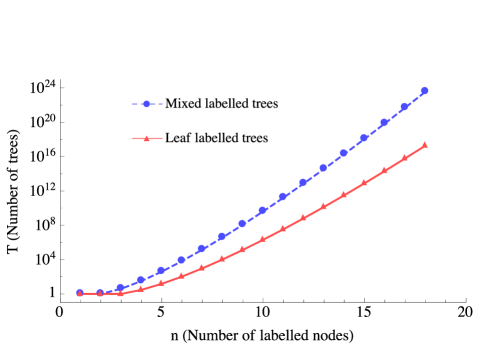
Figure 1: Comparison of growth rates of mixed and leaf labelled trees.

4 Maximum Parsimony for trees with labelled leaves

According to the parsimony criterion, we seek a tree that explains divergence of species with the fewest number of evolutionary events. As such, we seek to identify a tree with $n$ labelled nodes and fitted unlabelled nodes such that the tree cost, which is the sum of edge costs and therefore the total number of mutations, is minimized. This problem can be broken into two subproblems. Small parsimony problem (SPP): Given a tree $\tau$ with $n$ species nodes and a specified topology, compute its MP-cost. Large parsimony problem (LPP): Given a set of $n$ species, find the tree(s) with the minimum MP-cost among all possible tree topologies. Such tree(s) is/are called the most parsimonious tree(s) (MP-trees).

4.1 Hartigan’s algorithm

Hartigan’s algorithm provides a powerful framework for calculating best fits of a given tree. It solves the SPP for multifurcating rooted trees with $n$ labelled leaves [24]. The bottom-up procedure of Hartigan’s algorithm processes every unlabelled internal node $u_{i},1\leq i\leq n-2$ that has children $v_{i},i\geq 2.$ The procedure recursively calculates upper $VU(u)_{i}$ and lower $VL(u)_{i}$ sets for every character of every unlabelled node $u$ as follows (theorem 2 in [24]):

If $k(A)$ the number of times a value $A$ occurs in the sets $VU(u)_{i}$ of every child $v$ of $u$, and $K=\max{k(A)}$, then

1. $VU(u)_{i}=\{A|k(A)=K\}$

2. $VL(u)_{i}=\{A|k(A)=K-1\}$

Hartigan’s top down refinement allows the computation of optimal assignments to each node. For any character $i$ of the root node, selecting any of the candidate states from its root set would yield a most parsimonious labelling. The algorithm then proceeds to compute the root sets of characters of internal nodes $v$ using the following result (theorem 3 in [24]):

For $v$ child of $u$:

1. If $VV(u)_{i}\subseteq VU(v)_{i}$, then $VV(v)_{i}=VV(u)_{i}$

2. Otherwise, $VV(v)_{i}=VU(v)_{i}\cup(VV(u)_{i}\cap VL(v)_{i})$

By storing all optimal and next-to-optimal values in sets $VU(u)$ and $VL(u)$ respectively, and by computing $VV(u)$, Hartigan’s algorithm can be used to find all co-optimal solutions to the SPP. An example of Hartigan’s algorithm can be seen in Fig. 2.

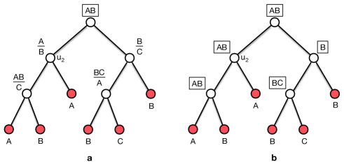
Figure 2: Hartigan’s algorithm: (a) Computation of upper $VU$ and lower $VL$ sets of all unlabelled nodes, as well as root $VV$ set of root node, after bottom-up step. (b) Computation of root sets $VV$ of all unlabelled nodes after top-down step.

4.2 Unrooting trees

Tree enumeration for the LPP on rooted full binary trees involves the systematic generation of cubic trees, for which MP-costs are computed by arbitrarily rooting the trees. To maintain bifurcation, a root can be added to a tree by replacing an edge $(v_{1},v_{2})$ with a new unlabelled root node $r$ and two edges $(r,v_{1})$ and $(r,v_{2})$. It is evident that the cost of the new tree will remain unaltered, since the root node can be assigned the same root set and value as one of either $v_{1}$ or $v_{2}$.

Conversely, the following theorem also holds true:

Theorem 1.

Removing the root of a binary tree, as well as any unlabelled node of degree 2, does not change the MP-cost of the tree.

Proof.

Hartigan’s algorithm on a rooted binary tree computes the root sets of all internal nodes, including the root set $VV(r)$ of the root node $r$. Let $VV(x)$ and $VV(y)$ be the corresponding root sets of the root’s children $x$ and $y$. Any assignment of a state $S_{i}\in VV(r)_{j}$ to the character $C_{j}$ of the root node will result in

1. A cost of $0$ for mutating this character from the root to both children, if $VV(r)_{j}\in(VV(x)_{j}\cap VV(y)_{j})$ or

2. A cost of $1$ otherwise (when $VV(r)_{j}\in(VV(x)_{j}\cup VV(y)_{j}$)).

Removing the root and connecting nodes $x$ and $y$ directly with an edge will not cause an increase to the MP-cost of the tree, as the same assignments that would minimize the edge costs between the root and its children will now be maintained on the edge $(x,y)$, meaning $0$ for each character $j$ whose state does not mutate ($VV(x)_{j}\cap VV(y)_{j}\neq\emptyset$), and $1$ when the state mutates. ∎

Therefore, cubic trees with $n$ labelled leaves share the same MP-cost with binary rooted counterparts (not necessarily full).

5 Towards a compact most parsimonious tree

Our ultimate goal is to find the most compact parsimonious $n$-species trees. To solve this problem, in this section we will demonstrate that it is sufficient to find the cubic $n$-species MP-trees and contract them. Towards that goal we will prove that most compact $n$-species MP-tree cannot have a lower cost fit than the cubic $n$-species MP-tree. To prove this claim we will utilize the following lemmas:

Lemma 1.

An $n$-species MP-tree with labelled internal nodes cannot have a lower cost than an $n$-species MP-tree with $n$ labelled leaves.

Proof.

We will prove by construction, while maintaining the invariant of lowest tree cost. Consider an $n$-species MP-tree with labelled internal nodes. Let $u_{i}$ be one of these nodes. Let $(u_{i},v)$ be an edge connecting $u_{i}$ with another node $v$. We will create a new internal node $u_{k}$ with the same root set as $u_{i}$, meaning $VV(u_{k})=VV(u_{i})$. We will then remove the $(u_{i},v)$ edge and connect $u_{k}$ to $u_{i}$ and $v$ with two edges $(u_{i},u_{k})$ and $(u_{k},v)$. We will then create a new leaf node $u_{l}$ with $VV(u_{l})=VV(u_{i})$ and connect it to node $u_{k}$ with an edge $(u_{k},u_{l})$. Finally we will move the label from $u_{i}$ to $u_{l}$, effectively removing a labelled internal node and creating a labelled leaf. The construction is shown in Fig. 3.

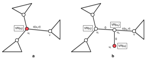
Figure 3: Moving an internal labelled node to a leaf while maintaining tree cost

The tree cost remains unchanged during these operations, since edge $(u_{k},v)$ will have the same potential cost (for the same fit of $v$) as edge $(u_{i},v)$ had, where the other new edges $(u_{i},u_{k})$ and $(u_{k},u_{l})$ will have potential costs of $0$, since they connect nodes with the same single-fit root sets. We can repeat this process independently on every internal labelled node, until the only labelled nodes are leaves, while the MP-cost of the tree remains the same. ∎

Lemma 2.

In leaf-labelled trees, a multifurcating $n$-species MP-tree cannot have a lower cost fit than an $n$-species cubic MP-tree.

Proof.

We will prove this lemma by construction, once again without modifying the MP-tree cost. A multifurcating tree has two types of nodes that do not appear in a cubic tree, nodes of degree $2$ and nodes of degrees $\geq 4$. We have seen how to remove unlabelled nodes of degree 2 in Theorem 1 without increasing the MP-tree cost. To remove tree nodes with degrees greater than $3$ we will introduce a split operation that will create a new node, reduce the degree of an existing node by $1$, and conserve the tree cost.

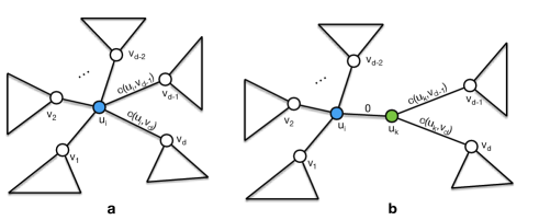
Figure 4: Node split to reduce degree of a node while maintaining tree cost

Consider a node $u_{i}$ with degree $d>3$. Node $u_{i}$ will be adjacent to $d$ other nodes $v_{1},v_{2},\dots,v_{d}$. We will create a new unlabelled node $u_{k}$ with the same root set as $u_{i}$, which we will connect to $u_{i}$. Then we will disconnect nodes $v_{d-1}$ and $v_{d}$ from $u_{i}$, and connect them to $u_{k}$. The modified node $u_{i}$ is now connected to nodes $v_{1},v_{2},\dots,v_{d-2},u_{k}$ and has degree $d-1$, where node $u_{k}$ is adjacent to $u_{i},v_{d-1}$ and $v_{d}$, and has degree $3$. The degrees of all other nodes are unchanged. The MP-tree cost remains the same, as new edge $(u_{i},u_{k})$ has a potential cost of 0 with an original tree best fit, and removed edges $(u_{i},v_{d-1})$ and $(u_{i},v_{d})$ carry the same potential cost with added edges $(u_{k},v_{d-1})$ and $(u_{k},v_{d})$ respectively. The split operation is shown in Fig. 4.

Repeating the split operation on all nodes with degrees $\geq 4$ until their degrees are reduced to $3$ will produce a cubic tree with the same MP-cost as the original multifurcating tree. ∎

Lemma 3.

Unlabelled nodes with degrees $d<3$ can be removed from an $n$-species tree without increasing its MP-cost.

Proof.

We have seen how to remove unlabelled nodes of degree $2$ in Theorem 1 without increasing the tree MP-cost. To remove an unlabelled leaf $v$, we can notice that its incident edge can always have a cost of $0$ for any given fit, since we can always set $VV(v)=VV(u)$, where $u$ is the single neighbor of $v$. As such, removal of $v$ and its incident edge does not increase the tree cost. ∎

Lemma 4.

A most compact parsimonious $n$-species tree will have at most $n-2$ unlabelled nodes.

Proof.

Based on Lemma 3, all leaves of a most compact MP-tree will be labelled. Thus, such a tree will have $n$ leaves. Assume to the contrary of our stated lemma that a most compact $n$-species MP-tree has $k\geq n-1$ internal nodes, all of which have degrees $\geq 3$, as per Lemma 3. Then the total number of nodes of the tree is $n+k$. A tree with $n+k$ nodes has $n+k-1$ edges. The sum of the node degrees then will be $2n+2k-2$, since every edge contributes $2$ to the total sum.

The sum of the degrees of the $n$ leaves is $n$, which means that the sum of degrees of the internal nodes $S=n+2k-2$. Since every internal node has a degree $\geq 3$, the $k$ internal nodes will have a sum of degrees $S\geq 3k\Leftrightarrow n+2k-2\geq 3k\Leftrightarrow k\leq n-2$, which contradicts our assumption $k\geq n-1$. ∎

Now we can proceed with the proof of our main theorem:

Theorem 2.

The most compact $n$-species MP-tree cannot have a lower cost fit than the $n$-species cubic MP-tree.

Proof.

Assume to the contrary that there exists a tree $\tau_{c}$ on $n$ species $S$ that has a lower cost than the cubic MP-tree $\tau$ on $S$. Using the construction in Lemma 1 we can move all labelled internal nodes to leaves without increasing the MP-cost of $\tau_{c}$. Based on Lemma 4 we could remove all unlabelled nodes with degrees $\leq 2$ without altering the MP-cost of $\tau_{c}$ as well. Now $\tau_{c}$ has only nodes with degree $1$ or degree $\geq 3$. Using the construct of Lemma 2 we can convert $\tau_{c}$ to a cubic tree, by successively splitting nodes of degree higher than 3, again without affecting the MP-cost of $\tau_{c}$. The resulting tree is cubic, has all species in $S$ associated with leaves, and a lower cost than $\tau$. ∎

Theorem 2 enables us to build the most compact MP-tree without enumerating all $n$-species trees, but only cubic trees with $n$ species. It also supplies us with a systematic procedure to create the most compact parsimonious tree by reversing the process described in Theorem 2. Starting with the $n$-species cubic MP-trees, we can contract edges with $0$ min-cost, effectively reversing the split operation. But which is the right order to contract edges, so that we can produce the most compact parsimonious tree? The relation $R:V\to V:(u,v)\in R\iff md(u,v)=0$ is not transitive, and edge contraction order can matter. Therefore we will consider all possible orders of edge contractions.

Lemma 5.

The root tuple $VV(v)$ of a node $v$ is independent of the placement of the root of the tree and its character sets are maximal.

Proof.

$VV(v)$ indicates the tuple of maximal sets of states that can be assigned to corresponding characters of $v$ in a most parsimonious fit. These are computed by the top-down procedure of Hartigan’s algorithm , the correctness of which is proven in theorem 3 of [24]. ∎

Corollary 1.

$VV(v)=VU(v)$ when $v$ is placed on the root.

The following lemma will help us prove the correctness of our contraction algorithm.

Lemma 6.

Only edges with $0$ min-cost can be contracted without increasing tree cost.

Proof.

Assume to the contrary that we can contract an edge with min-cost $>0$ where the contracted tree $\tau_{c}$ has the same MP-cost $MM(\tau)$ as the initial MP-tree $\tau$. Let $(u,v)$ be such an edge. Then $\exists i,1\leq i\leq m:VV(v)_{i}\cap VV(u)_{i}=\emptyset$.

Let $w$ be the new node created once edge $(u,v)$ is contracted. A value $V(w)$ with $V(w)_{i}=x\in VV(u)_{i}$ (we select $u$ without loss of generality) would set $MM(\tau_{c})>MM(\tau)$. To see that, let us root $\tau$ at $u$. Clearly $VV(u)_{i}\not\subseteq VV(v)_{i}$, which means, based on theorem 2 of [24] and Lemma 5, that $VV(v)_{i}=VU(v)_{i}\cup(VV(u)_{i}\cap VL(v)_{i})$. But then $x\not\in VU(v)_{i}$, since $x\in VU(v)_{i}\implies x\in VV(v)_{i}\implies VV(v)_{i}\cap VV(u)_{i}\neq\emptyset$. Also $x\not\in VL(v)_{i}$, since $x\in VL(v)_{i}\implies x\in VV(u)_{i}\cap VL(v)_{i}\implies x\in VV(v)_{i}\implies VV(v)_{i}\cap VV(u)_{i}\neq\emptyset$. Thus an assignment of $x$ to $V(v)_{i}$ in $\tau$ would increase the cost of the subtree rooted at $v$ by $2$ more than any other assignment from $VV(v)_{i}=VU(v)_{i}$. Even with the gain of one mutation from the contraction of edge $(u,v)$, $MM(\tau_{c})>MM(\tau)$, which is a contradiction. ∎

Corollary 2.

After an edge $(u,v)$ contraction, the new node $w$ will have root set $VV(w):\forall_{i}1\leq i\leq m,VV(w)_{i}=VV(u)_{i}\cap VV(v)_{i}$.

Proof.

The proof follows from the same process as in Lemma 6. ∎

Our algorithm for contracting a cubic tree to the most compact tree on $n$ species with the same cost is described in Algorithm 1.

Algorithm 1 Tree contraction algorithm

1:loop For each $0$-min-cost edge

2:     Contract edge $(u,v)$, remove $u,v$ and create new node $w$

3:     Update root set of w: $\forall_{i}1\leq i\leq mVV(w)_{i}=VV(u)_{i}\cap VV(v)_{i}$

4:     Root tree on w and run DFS to:

5:     (a) Update root sets of all unlabelled tree nodes and

6:     (b) Update list of $0$-min-cost edges

Theorem 3.

Algorithm 1 yields the most compact parsimonious tree

Proof.

The proof of correctness of Algorithm 1 follows from the reversal of the conversion of the most compact MP-tree to a cubic MP-tree. We are exhaustively enumerating all $n$-species cubic trees and, for the most parsimonious of them, we are considering all possible orders of edge contractions. Contracting edges reverses the node split operation that was utilized in Theorem 2. ∎

The initial cubic tree (before any contractions) has $n$ labelled and $n-2$ unlabelled nodes, therefore $2n-2$ nodes and $2n-3$ edges. The minimum number of nodes a compact tree can have is $n$, so the maximum number of consecutive contractions that can be performed is $n-2$. In the worst case our algorithm can iterate $(2n-3)(2n-4)\cdot\dots\cdot n=\binom{2n-3}{n-2}$ times. Each iteration involves a DFS traversal that takes linear time as a function of the size of the tree. Therefore the worst-case time complexity of the edge contraction algorithm is hyperexponential. Previous work in tree refinement, where maximum parsimony is pursued by contracting edges in trees, has shown that the tree refinement problem is NP-hard [27], indicating that our problem may not have efficient solutions in the worst case without bounding the values of any parameters. On average we would expect the edge contraction algorithm to be much more efficient, as the probability of contracting a tree edge decreases exponentially as a function of the number of characters examined, assuming character independence.

6 Experimental Results

Table I: Mixed Tree Enumeration vs Cubic MP-Tree Contraction

Number of	MTEA	CTEECA	Compact Mixed	Cubic	Contracted Cubic	Number of
Species	Time (ms)	Time (ms)	MP-Trees (#)	MP-Trees (#)	MP-Trees (#)	Contractions
4	10	8	1.1	1.1	3	1.4
5	36	10	1.6	1.9	5.4	1.7
6	191	43	2	2.7	13.4	1.8
7	796	167	3.5	4.4	162	2.3
8	8540	811	2.5	4	30.2	2.4
9	128242	10458	4.8	10.5	328.8	2.8
10	865839	139922	5.2	10.1	752	3.1
11	3831436	1778987	3.9	18.7	1716.8	3.5

We implemented two branch-and-bound algorithms to identify the most compact MP-trees for $n$ species. The first algorithm, the Mixed Tree Enumeration Algorithm (MTEA), exhaustively enumerates all mixed trees to identify the most compact MP-trees. The second algorithm, the Cubic Tree Enumeration and Edge Contraction Algorithm (CTEECA), exhaustively enumerates all cubic trees to find the MP-trees, on which it applies our edge contraction method to identify the most compact MP-trees.

We run these two algorithms on a dataset of viral sequences from the genes lef-8 and ac22 of the Baculoviridae family, analyzed in [28]. A multiple alignment of these sequences was downloaded from TreeBASE [29], and the first 30 characters of each taxon were used. We excluded 4 taxa for which the first 30 characters were not known.

We run our two algorithms to find most compact MP-trees for $n$ species with $4\leq n\leq 11$. The $n$ species were selected at random from the 35 available sequences, and for each value of $n$ we run 10 seperate randomized experiments, averaging the results. All experiments were run on a desktop computer with an Intel i7-4820k processor running at 3.7Ghz with 16 GB of RAM, an amount adequate for all data to be stored in memory once the input sequences were imported from the solid state drive.

The results of our experiments are shown in Table I. Execution times displayed include the time needed to enumerate and score mixed trees, or the time needed to enumerate, score, and contract cubic trees. Running times varied significantly among trials for any given $n$, due to the nature of branch and bound algorithms; in some trials, low scoring trees were found earlier on in the enumeration, allowing for more efficient pruning of the search space. The number of compact mixed trees reported is the mean number of most parsimonious mixed trees that had the fewest number of nodes. The number of most compact trees from the cubic enumeration includes all possible most compact trees generated by contracting edges in the most parsimonious cubic trees. This comparatively high number includes possible duplicate trees as well as possible rerootings of the same tree. The number of contractions is the mean number of zero min-cost edges that were contracted in the most parsimonious cubic trees. This shows the average difference in the number of nodes between the most compact trees and the cubic trees from which they were generated. Our results experimentally demonstrate that the CTEECA outperforms the MXEA by at least an order of magnitude on reasonable biological datasets, with similar behavior observed on datasets from the domain of phylogenetic stemmatics.

The programs used to perform these experiments were written in the Java programming language and the documented source code be downloaded at: https://github.com/ottj3/phylotreecontract.

7 Conclusion

In this work we have established a novel connection between mixed MP-trees and cubic MP-trees, and shown a mapping from the cubic MP-trees to the most compact mixed MP-trees, enabling more efficient algorithms for live phylogeny with polytomies. We have designed and implemented an efficient optimal algorithm to generate the most compact MP-trees for $n$ species by enumerating all cubic $n$-species trees, finding the most parsimonious ones, and optimally contracting them. Although contraction requires potentially hyper-exponential time as a function of the number of species, the running time of our algorithm is superior to the enumeration of all multifurcating trees with $n$ species, even in the worst case. On average we expected the contraction algorithm to be comparatively very efficient, an expectation that was confirmed experimentally. Furthermore, cubic tree enumeration has been refined in several existing phylogenetic software suites for many years [30, 31], and a large number of heuristics, approximations, and parallel algorithms have been developed and used effectively to speed up enumeration [27, 17, 32, 33, 34, 35, 36, 37], advancements of which our edge contraction algorithm can easily take advantage to further improve its efficiency.

It is our hope that our theoreticaly advances in the understanding of maximum live parsimony with polytomies and our optimal algorithms for identifying the most compact MP-trees for $n$ species – providing the ability to handle polytomies and input species on internal nodes natively – will enhance studies and enable new advances in evolutionary virology, paleontology, linguistics, and phylogenetic stemmatics.

References

- [1] J. Huelsenbeck and F. Ronquist, “Mrbayes: Bayesian inference of phylogenetic trees,” Bioinformatics, vol. 17, no. 8, pp. 754–755, 2001. [Online]. Available: http://www.ncbi.nlm.nih.gov/pubmed/11524383
- [2] J. Felsenstein, “Evolutionary trees from DNA sequences: A maximum likelihood approach,” Journal of Molecular Evolution, vol. 17, no. 6, pp. 368–376, 1981.
- [3] D. Hillis, J. Bull, M. White, M. Badgett, and I. Molineux, “Experimental phylogenetics: generation of a known phylogeny,” Science, vol. 255, no. 5044, pp. 589–592, 1992.
- [4] T. Zhu, B. Korber, A. Nahmias, E. Hooper, P. Sharp, and D. Ho, “An african hiv-1 sequence from 1959 and implications for the origin of the epidemic,” Nature, vol. 391, no. 6667, pp. 594–597, 1998.
- [5] R. Bush, C. Bender, K. Subbarao, N. Cox, and W. Fitch, “Predicting the evolution of human influenza A,” Science, vol. 286, no. 5446, pp. 1921–1925, 1999. [Online]. Available: http://www.ncbi.nlm.nih.gov/pubmed/10583948
- [6] G. D. Wilson and G. D. Edgecombe, “The triassic isopod protamphisopus wianamattensis (chilton) and comparison with extant taxa (crustacea, phreatoicidea),” Journal of Paleontology, vol. 77, no. 3, pp. 454–470, 2003. [Online]. Available: http://www.jstor.org/stable/pdf/4094794.pdf?seq=1#page_scan_tab_contents
- [7] N. Salamin, T. R. Hodkinson, and V. Savolainen, “Building supertrees: an empirical assessment using the grass family (Poaceae).” Systematic biology, vol. 51, no. 1, pp. 136–150, 2002.
- [8] D. L. Swofford and J. Sullivan, “Phylogeny inference based on parsimony and other methods using PAUP,” in The Phylogenetic Handbook, 2nd ed., P. Lemey, M. Salemi, and A.-M. Vandamme, Eds. Cambridge University Press, 2009, pp. 267–312, cambridge Books Online. [Online]. Available: http://dx.doi.org/10.1017/CBO9780511819049.010
- [9] G. P. Telles, N. F. Almeida, R. Minghim, and M. E. M. T. Walter, “Live phylogeny.” Journal of computational biology : a journal of computational molecular cell biology, vol. 20, no. 1, pp. 30–7, 2013. [Online]. Available: http://www.ncbi.nlm.nih.gov/pubmed/23294270
- [10] S. A. Carroll, J. S. Towner, T. K. Sealy, L. K. McMullan, M. L. Khristova, F. J. Burt, R. Swanepoel, P. E. Rollin, and S. T. Nichol, “Molecular evolution of viruses of the family filoviridae based on 97 whole-genome sequences,” Journal of Virology, vol. 87, no. 5, pp. 2608–2616, 2013. [Online]. Available: http://jvi.asm.org/content/87/5/2608.abstract
- [11] P. Buendia and G. Narasimhan, “Serial evolutionary networks of within-patient HIV-1 sequences reveal patterns of evolution of X4 strains.” BMC Systems Biology, vol. 3, p. 62, 2009.
- [12] M. Foote, “On the probability of ancestors in the fossil record,” Paleobiology, vol. 22, pp. 141–151, 1996. [Online]. Available: http://journals.cambridge.org/article_S0094837300016146
- [13] P. Mierzejewski, “A new graptolite, intermediate between the tuboidea and the. camaroidea,” Acta Palaeontologica Polonica, vol. 46, no. 3, pp. 367–376, 2001. [Online]. Available: https://www.app.pan.pl/archive/published/app46/app46-367.pdf
- [14] A. Urbanek, “Oligophyly and evolutionary parallelism: A case study of silurian graptolites,” Acta Palaeontologica Polonica, vol. 43, no. 4, pp. 549–572, 1998.
- [15] D. W. Bapst, “paleotree: an R package for paleontological and phylogenetic analyses of evolution,” Methods in Ecology and Evolution, vol. 3, no. 5, pp. 803–807, 2012. [Online]. Available: http://dx.doi.org/10.1111/j.2041-210X.2012.00223.x
- [16] A. F. Y. Poon, L. W. Walker, H. Murray, R. M. McCloskey, P. R. Harrigan, and R. H. Liang, “Mapping the Shapes of Phylogenetic Trees from Human and Zoonotic RNA Viruses,” PLoS ONE, vol. 8, no. 11, pp. 78–122, 2013. [Online]. Available: http://dx.doi.org/10.1371%2Fjournal.pone.0078122
- [17] P. A. Goloboff, “Optimization of polytomies: state set and parallel operations.” Molecular phylogenetics and evolution, vol. 22, no. 2, pp. 269–275, 2002.
- [18] R. L. Graham and L. R. Foulds, “Unlikelihood that minimal phylogenies for a realistic biological study can be constructed in reasonable computational time,” Mathematical Biosciences, vol. 60, no. 2, pp. 133–142, 1982.
- [19] W. H. E. Day, “Computationally difficult parsimony problems in phylogenetic systematics,” Journal of Theoretical Biology, vol. 103, no. 3, pp. 429–438, 1983.
- [20] W. H. E. Day, D. S. Johnson, and D. Sankoff, “The computational complexity of inferring rooted phylogenies by parsimony,” Mathematical Biosciences, vol. 81, no. 1, pp. 33–42, 1986.
- [21] A. Carmel, N. Musa-Lempel, D. Tsur, and M. Ziv-Ukelson, “The worst case complexity of maximum parsimony,” in Lecture Notes in Computer Science (including subseries Lecture Notes in Artificial Intelligence and Lecture Notes in Bioinformatics), vol. 8486 LNCS, 2014, pp. 79–88.
- [22] C. Semple and M. Steel, Phylogenetics, ser. Oxford lecture series in mathematics and its applications. Oxford University Press, 2003. [Online]. Available: https://books.google.gr/books?id=uR8i2qetjSAC
- [23] G. Exoo, “A simple method for constructing small cubic graphs of girths 14, 15, and 16.” The Electronic Journal of Combinatorics, vol. 3, no. 1, p. 30, 1996. [Online]. Available: http://eudml.org/doc/119250
- [24] J. A. Hartigan, “Minimum mutation fits to a given tree,” Biometrics, vol. 29, no. 1, pp. 53–65, 1973. [Online]. Available: http://www.jstor.org/stable/2529676
- [25] C. Flight, “How many stemmata?” Manuscripta, vol. 34, no. 2, pp. 122–128, 1990. [Online]. Available: http://dx.doi.org/10.1484/J.MSS.3.1335
- [26] N. Sloane. (2010) The On-Line Encyclopedia of Integer Sequences. [Online]. Available: http://oeis.org
- [27] M. Bonet, M. Steel, T. Warnow, and S. Yooseph, “Better methods for solving parsimony and compatibility,” J Comput Biol, vol. 5, no. 3, pp. 391–407, 1998. [Online]. Available: http://www.ncbi.nlm.nih.gov/pubmed/9773340
- [28] E. a. Herniou, J. a. Olszewski, D. R. O’Reilly, and J. S. Cory, “Ancient coevolution of baculoviruses and their insect hosts.” Journal of virology, vol. 78, no. 7, pp. 3244–3251, 2004.
- [29] W. H. Piel, M. Donoghue, and M. Sanderson, “TreeBASE : A database of phylogenetic information,” in Proceedings of the 2nd International Workshop of Species 2000, 2002, pp. 41–47. [Online]. Available: http://phylogeny.harvard.edu/treebase.
- [30] J. Felsenstein, “Phylip: phylogeny inference package (version 3.2),” Cladistics, vol. 5, pp. 164–166, 1989.
- [31] D. L. Swofford, “Phylogenetic Analysis Using Parsimony,” Options, vol. 42, pp. 294–307, 2003. [Online]. Available: http://www.springerlink.com/index/10.1007/BF02198856
- [32] M. Yan and D. A. Bader, “D.a.: Fast character optimization in parsimony phylogeny reconstruction,” Georgia Institute of Technology, Tech. Rep., 2003.
- [33] D. A. Bader, V. P. Chandu, and M. Yan, “ExactMP: An efficient parallel exact solver for phylogenetic tree reconstruction using maximum parsimony,” in Proceedings of the International Conference on Parallel Processing, 2006, pp. 65–73.
- [34] S. Sridhar, F. Lam, G. E. Blelloch, R. Ravi, and R. Schwartz, “Mixed integer linear programming for maximum-parsimony phylogeny inference,” in IEEE/ACM Transactions on Computational Biology and Bioinformatics, vol. 5, no. 3, 2008, pp. 323–331.
- [35] A. Goeffon, J. M. Richer, and J. K. Hao, “Progressive tree neighborhood applied to the maximum parsimony problem,” IEEE/ACM Transactions on Computational Biology and Bioinformatics, vol. 5, no. 1, pp. 136–145, 2008.
- [36] N. Alon, B. Chor, F. Pardi, and A. Rapoport, “Approximate maximum parsimony and ancestral maximum likelihood,” IEEE/ACM Transactions on Computational Biology and Bioinformatics, vol. 7, no. 1, pp. 183–187, 2010.
- [37] W. T. J. White and B. R. Holland, “Faster exact maximum parsimony search with XMP,” Bioinformatics, vol. 27, no. 10, pp. 1359–1367, 2011.