Impulse-induced localized control of chaos in starlike networks

Abstract

Locally decreasing the impulse transmitted by periodic pulses is shown to be a reliable method of taming chaos in starlike networks of dissipative nonlinear oscillators, leading to both synchronous periodic states and equilibria (oscillation death). Specifically, the paradigmatic model of damped kicked rotators is studied in which it is assumed that when the rotators are driven synchronously, i.e., all driving pulses transmit the same impulse, the networks display chaotic dynamics. It is found that the taming effect of decreasing the impulse transmitted by the pulses acting on particular nodes strongly depends on their number and degree of connectivity. A theoretical analysis is given explaining the basic physical mechanism as well as the main features of the chaos-control scenario.

I
INTRODUCTION

Controlling the dynamical state of a complex network is a fundamental problem in science [1-5] with many potential applications, including neuronal disorders in brain networks [6] and evaluation of risks in financial markets [7]. While most of these works consider networks of linear systems [1,2,5], only recently has the general and richer case of networks of nonlinear systems [4] started to be investigated. Here we are interested in controlling networks in the sense of driving the network from a subset of particular chaotic initial states to a subset of final (stable) regular states with the view of not merely identifying driver nodes but also their relative effectiveness as well as obtaining estimates of the regions in parameter space where suitable control signals are effective. Regarding the control (suppression and enhancement) of chaotic states, which is of fundamental interest partly because of the ubiquity of chaos in nature, including man-made systems, and partly because of its practical relevance [8-10], it has been shown that the application of judiciously chosen periodic external excitations is a reliable procedure for taming chaos in diverse coupled systems such as arrays of electrochemical oscillators [11], Frenkel-Kontorova chains [12], and recurrent neural networks [13], just to cite a few instances. Most studies of coupled nonlinear systems subjected to external excitations have focused on either global (all-to-all) or local (homogeneous) diffusive-type coupling, while little attention has been paid to the possible influences of a heterogeneous connectivity on the regularization of a network’s dynamics.

Many diverse real-world networks exhibit heterogeneous connectivity in the form of a scale-free topology [14] which means that just a small set of nodes are highly connected $-$the so-called hubs$-$ while the rest of the nodes have few connections. Since starlike structures are the main motifs of scale-free networks, here we study the control of chaos in starlike networks of dissipative driven nonlinear oscillators, expecting that the main features of such an impulse control scenario may be extensible to the case of scale-free networks. This is a major motivation for the present work. Chaos control and synchronization are deeply related phenomena [9], and there have been recent studies of diverse synchronization phenomena in oscillator networks with starlike couplings [15-18].

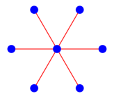
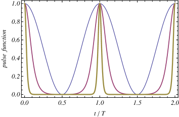
Figure 1: (Color online) Top: Schematic representation of a starlike network of $N=7$ rotators. Bottom: Pulse function $p(t;T,m)\equiv\operatorname{cn}^{2}\left[2K(m)t/T;m\right]$ [cf. Eq. (1)] versus $t/T$ for $m=0$ (thin line), $m=0.999$ (medium line), and $m=1-10^{-14}$ (thick line). The quantities plotted are dimensionless.

We shall consider a topology-induced chaos-control scenario in starlike networks of dissipative non-autonomous systems subjected to local chaos-suppressing (CS) external excitations. Specifically, the findings will be discussed through the analysis of starlike networks of $N$ damped kicked rotators (DKRs) – see Fig. 1 top. This system is sufficiently simple to allow analytical predictions while retaining the universal characteristics of a dissipative chaotic system. The complete model system reads

$$\overset{..}{x}_{H}+\operatorname{cn}^{2}\left(\Omega_{H}t;m_{H}\right)\sin x_{H} =-\delta\overset{.}{x}_{H}+\lambda\sum_{i=1}^{N-1}\sin\left(x_{i}-x_{H}\right),$$

$$\overset{..}{x}_{i}+\operatorname{cn}^{2}\left(\Omega_{i}t;m_{i}\right)\sin x_{i} =-\delta\overset{.}{x}_{i}+\lambda\sin\left(x_{H}-x_{i}\right),$$ (1)

$i=1,...,N-1$, and where all variables and parameters are dimensionless: $\Omega_{H,i}=\Omega_{H,i}\left(T,m_{H,i}\right)\equiv 2K(m_{H,i})/T$, $T$ is the common excitation period, $\delta$ is the damping coefficient, $\lambda$ is the coupling constant, $\operatorname{cn}\left(\cdot;m\right)$ is the Jacobian elliptic function of parameter $m$, and $K(m)$ is the complete elliptic integral of the first kind. Equations (1) describe the dynamics of a highly connected rotator (or hub), $x_{H}$, and $N-1$ linked rotators (or leaves), $x_{i}$. The shape parameter is taken to be $m=0$ except for certain sets of rotators that are subjected to pulses of variable width $\left(m\in\left[0,1\right]\right)$. The effect of renormalization of the elliptic cosine argument is clear: with $T$ constant, solely the pulse’s wave form is varied by changing $m$ between $0$ and $1$. Increasing $m$ makes the pulse narrower, and for $m\simeq 1$ one recovers a periodic sharply kicking excitation very close to the periodic $\delta$ function, but with finite amplitude and width (see Fig. 1 bottom). Also, $\operatorname{cn}^{2}\left(\Omega t;m=0\right)=\cos^{2}\left(\pi t/T\right)$, while at the other limit, $m=1$, the pulse area vanishes. It is worth mentioning that the limiting case $m=\delta=\lambda=0$ corresponds to an isolated Hamiltonian kicked rotator subjected to trigonometric pulses, which has been used to describe the center-of-mass motion of cold atoms in an amplitude-modulated standing wave of light [19], and that numerical studies have shown the suppressory effectiveness of decreasing the impulse transmitted by localized periodic pulses in homogeneous chains of DKRs [20].

Here we describe theoretical and numerical studies of the new chaos-control scenario arising from Eq. (1) by assuming parameter values such that each isolated rotator driven by trigonometric pulses $\left(m_{H}=m_{i}=0,i=1,...,N-1\right)$ displays chaotic behavior characterized by a positive Lyapunov exponent [21,22]. The remainder of the communication is organized as follows. Section II studies both the chaotic dynamics and the oscillation death (OD) [23] of isolated rotators (Eq.(1) with $\lambda=0$). Analytical estimates of the chaotic threshold in parameter space are obtained by using Melnikov’s method (MM) [24,25], while the phenomenon of OD is anticipated theoretically with the aid of an energy analysis. The interplay between heterogeneous connectivity and local decrease of the pulse’s impulse in networks described by Eq. (1) is discussed in Sec. III. We characterize a fairly complex regularization scenario, and determine how the effectiveness of the local reshaping of pulses depends upon the number of control nodes and their degree of connectivity. Finally, Sec. IV is devoted to a discussion of the major findings and to some concluding remarks.

II DYNAMICS OF ISOLATED ROTATORS

Before considering the chaos-control scenario of DKRs coupled in a starlike topology, it is necessary to understand the main features of the dynamics of an isolated DKR:

$$\overset{..}{x}+\operatorname{cn}^{2}\left(\Omega t;m\right)\sin x=-\delta\overset{.}{x}.$$ (2)

In particular, we are interested in obtaining an analytical estimate of the order-chaos threshold in parameter space, and in providing a theoretical argument showing that the equilibrium $\left(x=0,\overset{.}{x}=0\right)$ may be a stable attractor of Eq. (2) for pulses of a (certain) finite width $\left(m<1\right)$. For the sake of clarity, we shall consider these analyses separately.

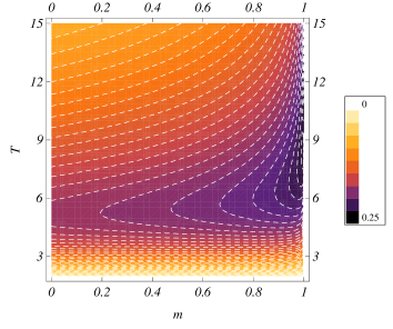
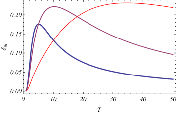
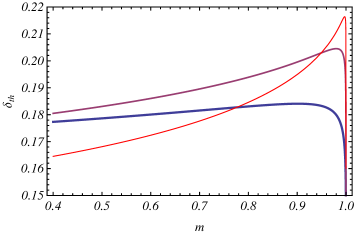
Figure 2: (Color online) Top: Contour plot of the chaotic threshold damping $\delta_{th}\left(T,m\right)$ [cf. Eq. (7)] vs shape parameter $m$ and period $T$. Middle: Chaotic threshold damping $\delta_{th}\left(T,m\right)$ [cf. Eq. (7)] vs period $T$ for $m=0$ (thick line), $m=0.999$ (medium line), and $m=1-10^{-14}$ (thin line). Bottom: Chaotic threshold damping $\delta_{th}\left(T,m\right)$ [cf. Eq. (7)] vs period $m$ for $T=4.5$ (thick line), $T=6$ (medium line), and $T=8$ (thin line). The quantities plotted are dimensionless.

II.1 Order-chaos threshold

To obtain analytical estimates of the chaotic threshold in parameter space $\left(T,m,\delta\right)$, we first note that Eq. (2) can be recast into the form

$$\overset{..}{x}+\sin x=-\delta\overset{.}{x}+\operatorname{sn}^{2}\left(\Omega t;m\right)\sin x,$$ (3)

where $\operatorname{sn}\left(\cdot;m\right)$ is the Jacobian elliptic function of parameter $m$, and assume that the DKR (3) satisfies the MM requirements, i.e., the dissipation and parametric excitation terms are small-amplitude perturbations of the underlying conservative pendulum $\overset{..}{x}+\sin x=0$. Melnikov introduced a function (the so-called Melnikov function (MF), $M\left(t_{0}\right)$) which measures the distance between the perturbed stable and unstable manifolds in the Poincaré section at $t_{0}$. If the MF presents a simple zero, the manifolds intersect transversally and chaotic instabilities result. See Refs. [24,25] for more details about MM. Regarding Eq. (3), note that, in keeping with the assumption of the MM [24,25], it is assumed that one can write $\delta=\varepsilon\overline{\delta},$ where $0<\varepsilon\ll 1$ while $\overline{\delta}$ is of order unity. The term $\operatorname{sn}^{2}\left(\Omega t;m\right)\sin x$ in Eq. (3) is not $O\left(\varepsilon\right)$, and one should not consider it to be a perturbative term. However, this will be assumed in calculating the MF so as to obtain an effective (qualitative) estimate of the chaotic threshold in parameter space which may be useful in explaining the results of the numerical experiments. Thus, bearing in mind this caveat, the application of MM to Eq. (3) yields the MF

$$M^{\pm}\left(t_{0}\right) =-D+\sum_{n=1}^{\infty}a_{n}\left(m\right)b_{n}\left(T\right)\sin\left(\frac{2n\pi t_{0}}{T}\right),$$

$$D \equiv 8\delta,$$

$$a_{n}\left(m\right) \equiv\frac{2n\pi^{3}}{mK^{2}(m)}\operatorname{csch}\left[\frac{n\pi K(1-m)}{K(m)}\right],$$

$$b_{n}\left(T\right) \equiv\frac{4n^{2}\pi^{2}}{T^{2}}\operatorname{csch}\left(\frac{n\pi^{2}}{T}\right),$$ (4)

where the positive (negative) sign refers to the top (bottom) homoclinic orbit of the underlying conservative pendulum

$$\theta_{0}\left(t\right) =\pm 2\arctan\left[\sinh\left(t\right)\right],$$

$$\overset{.}{\theta}_{0}\left(t\right) =\pm 2\operatorname{sech}\left(t\right).$$ (5)

If $M^{\pm}\left(t_{0}\right)$ has a simple zero, then a heteroclinic bifurcation occurs, signifying the onset of chaotic instabilities. From Eq. (4) one sees that

$$\sum_{n=1}^{\infty}a_{n}\left(m\right)b_{n}\left(T\right)\sin\left(2n\pi t_{0}/T\right)\leqslant\sum_{n=1}^{\infty}a_{n}\left(m\right)b_{n}\left(T\right).$$

If the damping coefficient is such that

$$D\geqslant\sum_{n=1}^{\infty}a_{n}\left(m\right)b_{n}\left(T\right),$$

this relationship represents a sufficient condition for $M^{\pm}\left(t_{0}\right)$ to always have the same sign, i.e., $M^{\pm}\left(t_{0}\right)\leqslant 0$. Thus, a necessary condition for $M^{\pm}\left(t_{0}\right)$ to change sign at some $t_{0}$ is written

$$\delta<\delta_{th}\left(T,m\right),$$ (6)

where the chaotic threshold damping scales as

$$\delta_{th}\left(T,m\right)\sim\frac{1}{8}\sum_{n=1}^{\infty}a_{n}\left(m\right)b_{n}\left(T\right).$$ (7)

From Eq. (7) one readily obtains

$$\lim_{T\rightarrow 0,\infty}\delta_{th}\left(T,m\right)=\lim_{m\rightarrow 1}\delta_{th}\left(T,m\right)=0,$$

i.e., in such limits chaotic dynamics is not expected. Also, one finds that $\delta_{th}\left(T,m\right)$ presents a maximum in the $m-T$ plane at $\left(m=m_{\max},T=T_{\max}\right)$. A plot of $\delta_{th}\left(T,m\right)$ is shown in Fig. 2 top. Let us consider the chaotic threshold damping as a function of $T$, holding $m$ constant. Plots of $\delta_{th}\left(T,m=const\right)$ show that each curve presents a maximum $T_{\max}=T_{\max}(m)$ such that $T_{\max}(m)$ increases from its value at $m=0$ as $m\rightarrow 1$ (see Fig. 2 middle). Now we study the chaotic threshold damping as a function of $m$, holding $T$ constant. Plots of $\delta_{th}\left(T=const,m\right)$ show that each curve presents a maximum $m_{\max}=m_{\max}(T)$ such that $m_{\max}(T)$ increases as $T$ is increased (see Fig 2 bottom). Thus, these MM-based predictions indicate that by sufficiently decreasing the impulse transmitted by the pulses (time integral over a period), i.e., when $m$ is sufficiently near $1$, is a reliable procedure for suppressing chaos irrespective of the values of the remaining parameters. Next, we compare the chaotic thresholds predicted from MM and Lyapunov exponent (LE) calculations. It is worth mentioning that we cannot expect too good a quantitative agreement between the two types of results because MM is generally related with transient chaos while LE provides information concerning only steady motions. We compute LEs by using a version of the algorithm introduced in Ref. [26]. We typically integrate up to $10^{4}$ drive cycles for fixed period $T=5.52$. In a first step, we calculate the leading LE for each point on a $100\times 100$ grid, with shape parameter $m$ and damping coefficient $\delta$ given by the horizontal and vertical axes, respectively. Second, we construct the diagram shown in Fig. 3 by only plotting a point on the grid when the respective leading LE is larger than $10^{-3}$. The chaotic threshold (solid line in Fig. 3) predicted from MM gives a qualitative estimate for the upper boundary of the entire chaotic region, as expected (recall the aforementioned caveats). Notwithstanding, the theoretical estimate captures two main features of the numerically obtained chaotic boundary: the existence of a maximum at a certain value of the shape parameter, $m_{\max}^{LE}$, and that the chaotic boundary exhibits a monotonously decreasing behavior as a function of the shape parameter from $m=m_{\max}^{LE}$. Note that the corresponding theoretically predicted maximum $m_{\max}=m_{\max}(T=5.52)$ is very close to $m_{\max}^{LE}$.

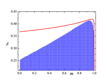
Figure 3: (Color online) Grid in the $m-\delta$ parameter plane for $T=5.52$. Dots indicate that the respective leading LE is larger than $10^{-3}$. The solid line denotes the theoretical estimate of the chaotic boundary $2.1\delta_{th}\left(T=5.52,m\right)$ [cf. Eq. (7)] from MM.

We will show in Sec. III how numerical simulations of starlike networks of DKRs confirmed the effectiveness of this chaos-control procedure.

II.2 Energy-based analysis

By analyzing the variation of the system’s kinetic energy, one straightforwardly predicts the occurrence of the phenomenon of OD. Indeed, Eq. (3) has the associated energy equation

$$\frac{dE_{K}}{dt}=-\delta\overset{.}{x}^{2}-\operatorname{cn}^{2}\left(\Omega t;m\right)\overset{.}{x}\sin x,$$ (8)

where $E_{K}(t)\equiv\left(1/2\right)\overset{.}{x}^{2}\left(t\right)$ is the kinetic energy function. Integration of Eq. (8) over any interval $\left[nT,nT+T\right]$, $n=0,1,2,...$, yields

$$E_{K}\left(nT+T\right) =E_{K}(nT)-\delta\int_{nT}^{nT+T}\overset{.}{x}^{2}\left(t\right)dt$$

$$-\int_{nT}^{nT+T}\operatorname{cn}^{2}\left(\Omega t;m\right)\dot{x}\left(t\right)\sin x(t)dt.$$ (9)

Now, after applying  the first mean value theorem for integrals [28] together with well-known properties of the Jacobian elliptic functions [27] to the last two integrals on the right-hand side of Eq. (9), one has

$$E_{K}\left(nT+T\right) =E_{K}(nT)-\delta\overset{.}{x}^{2}\left(t^{\ast\ast}\right)T$$

$$-\overset{.}{x}\left(t^{\ast}\right)\sin\left[x\left(t^{\ast}\right)\right]I\left(m\right)T,$$ (10)

where $t^{\ast},t^{\ast\ast}\in\left[nT,nT+T\right]$, while

$$I\left(m\right)\equiv\frac{E(m)+(m-1)K(m)}{mK(m)}$$ (11)

is the impulse transmitted over a period $T=1$ with $E(m)$ being the complete elliptic integral of the second kind. From Eq. (11) one straightforwardly obtains $I\left(m=0\right)=1/2,I\left(m=1\right)=0$. A plot of $I\left(m\right)$ is shown in Fig. 4. Now, if we consider fixing the parameters $\left(\delta,T\right)$ for the DKR to exhibit chaotic dynamics at $m=0$, there always exists an $n=n^{\ast}$ such that the kinetic energy increment

$$\Delta E_{K}^{m=0}\equiv E_{K}\left(n^{\ast}T+T\right)-E_{K}(n^{\ast}T)>0.$$

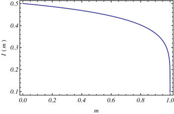
Figure 4: (Color online) Impulse function $I\left(m\right)$ versus shape parameter $m$ (cf. Eq. (11)). The quantities plotted are dimensionless.

In this situation, one decreases the impulse by increasing the shape parameter from $m=0$ while holding the remaining parameters constant. Equations (10) and (11) predict that, for each $n^{\ast}$, there always exists a minimum critical value $m=m_{c}>0$ such that the corresponding energy increment $\Delta E_{K}^{m=m_{c}}<0$ for all $n>n^{\ast}$, and hence the equilibrium $\left(x=0,\overset{.}{x}=0\right)$ is the single attractor of the DKR for $m\geqslant m_{c}$. Note that this property comes ultimately from the behavior of the impulse $I\left(m\right)$ as the shape parameter $m\rightarrow 1$ (see Fig. 4), i.e., that the DKR effectively behaves as a purely damped pendulum for sufficiently narrow pulses. Thus, one straightforwardly obtains from Eqs. (10) and (11) that, for sufficiently narrow pulses, the equilibrium $\left(x=0,\overset{.}{x}=0\right)$ is the single attractor of the DKR when $\delta>\delta_{c}$, where the critical damping coefficient scales as

$$\delta_{c}\sim I(m).$$ (12)

Numerical experiments confirmed the validity of this scaling for sufficiently narrow pulses, as in the example shown in Fig. 5.

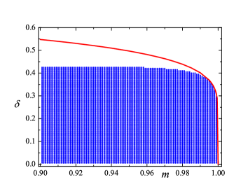
Figure 5: (Color online) Stability boundary of the equilibrium $\left(x=0,\overset{.}{x}=0\right)$ in the $m-\delta$ parameter plane for $T=5.52$. The instability region (dots) was numerically calculated on a grid of $100\times 100$ points. The solid line denotes the theoretical estimate of the stability boundary $\delta_{c}=1.5I(m)$ from Eq. (12). The quantities plotted are dimensionless.

III LOCALIZED CONTROL IN STARLIKE NETWORKS

In this section, we study the relative effectiveness of locally reshaping the pulses $\operatorname{cn}^{2}\left(\Omega t;m\right)$, in the sense of decreasing their impulse, on $M$ nodes of chaotic starlike networks of $N$ DKRs (cf. Eq. (1), $M<N$) while holding the remaining parameters constant. Before applying any control, we assume parameter values $\left(\delta,T\right)$ such that each isolated rotator driven by trigonometric pulses $\left(m_{H}=m_{i}=0,i=1,...,N-1\right)$ displays chaotic behavior. Equation (1) was numerically integrated using a fourth-order Runge-Kutta algorithm with a time step $\Delta t=0.001$. To visualize the global spatiotemporal dynamics of networks, we calculated the average velocity

$$\sigma\left(jT\right)\equiv\frac{1}{N}\sum_{i=1}^{N}\frac{dx_{i}}{dt}\left(jT\right),$$ (13)

where $j$ is an integer multiple of the pulse period $T$, while the degree of synchronization is characterized by the correlation function

$$C\equiv\frac{2}{N(N-1)}\sum_{\left(il\right)}\left\langle\cos\left(x_{i}-x_{l}\right)\right\rangle_{t},$$ (14)

with the summation being over all pairs of rotators, and where $\left\langle\cdot\right\rangle_{t}$ indicates time averaging over a predefined (sufficiently long) observation window. Note that $C$ is $1(0)$ for the perfectly synchronized (desynchronized) state. Calculations of LEs for the starlike networks [Eq. (1)] confirmed the reliability of the information provided by bifurcation diagrams of the average velocity $\sigma$ concerning transitions order-chaos. An illustrative example is shown in Fig. 6 for the case $N=10,M=5,\lambda=0.1,\delta=0.2,T=5.52$.

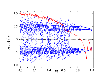
Figure 6: (Color online) Bifurcation diagrams of the average velocity $\sigma$ (blue (black) dots) and leading LE $\Lambda$ (red (gray) line) as a function of the shape parameter $m=m_{j}$ for the case of a central rotator subjected to trigonometric pulses $\left(m_{H}=0\right)$, $N=10,\lambda=0.1,\delta=0.2,T=5.52$, and $M=5$ peripheral rotators $x_{j}$ subjected to impulse control. The quantities plotted are dimensionless.

III.1 Control on a single peripheral rotator

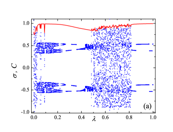
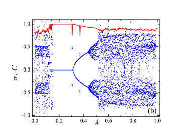
Figure 7: (Color online) Bifurcation diagrams of the average velocity $\sigma$ (blue (black) dots) and correlation function $C$ (red (gray) line) as a function of the coupling $\lambda$ for the case of a central rotator subjected to trigonometric pulses, $N=10,M=1,\delta=0.2,T=5.52$, and two values of the shape parameter: (a) $m_{j}=0.9$ and (b) $m_{j}=1-10^{-14}$. The quantities plotted are dimensionless.

Let us first consider the effect of decreasing the pulses’ impulse on a single peripheral rotator $x_{j}$ $\left(M=1\right)$ while the remaining rotators, including the hub, are subjected to trigonometric pulses $\left(m_{H}=m_{i}=0,i=1,...N-1,i\neq j\right)$. Note that this could be, a priori, the most unfavorable case in terms of completely regularizing the whole network. Numerical simulations indicate, however, that regularization to periodic states is possible over certain coupling intervals even for relatively wide pulses, such as for $m_{j}=0.9$ (see Fig. 7(a)), as expected from the above MM-based predictions. The symmetry of the bifurcation diagrams comes from the DKR’s symmetry with respect to the transformation $\left(x_{i}\rightarrow-x_{i}\right)$, i.e., if $\left[x_{i}(t),\overset{.}{x}_{i}\left(t\right)\right]$ is a solution of Eq. (1), then so is $\left[-x_{i}(t),-\overset{.}{x}_{i}\left(t\right)\right]$. The bifurcation diagram was constructed by means of a Poincaré map at the parameters indicated in the caption to Fig. 7. Starting at $\lambda=0$, and taking the transient time as $500$ pulse periods after every increment of $\Delta\lambda=3.3\times 10^{-3}$, we sampled $20$ pulse periods by picking up the first $\sigma$ values of every pulse cycle, while to obtain the correlation function [see Eq. (14)] we calculated $C$ averaged over $200$ additional pulse periods. In accordance with the above energy analysis, we typically find that the phenomenon of OD occurs over certain coupling intervals for sufficiently narrow pulses, the equilibrium $\left(x=0,\overset{.}{x}=0\right)$ being the asymptotic behavior of the perfectly synchronized network, as in the illustrative instance shown in Fig. 7(b) for $m_{j}=1-10^{-14}$. In general, the equilibrium $\left(x=0,\overset{.}{x}=0\right)$ becomes stable at a certain value $\lambda=\lambda_{\min}$ via a boundary crisis, while it becomes unstable at a certain higher value $\lambda=\lambda_{\max}$ via a supercritical Hopf bifurcation [29]. These threshold values of the coupling, $\lambda_{\max,\min}$, depend upon the remaining parameters. In particular, the dependence on the number of rotators $N$ of the width of the coupling interval in which OD occurs, $\Delta\lambda=\Delta\lambda\left(N\right)\equiv\lambda_{\max}\left(N\right)-\lambda_{\min}\left(N\right)$, follows a linear law, as is shown in Fig. 8. Note that $\Delta\lambda\rightarrow 0$ as $N$ approximates a sufficiently large but finite number of rotators. Besides the correlation function $C$, bifurcation diagrams of the average velocity $\sigma$ also provide useful information regarding the existence of multistability [30] over certain ranges of parameters. In the present case of starlike networks which are sufficiently far from the Hamiltonian limiting case, multistability comes from the conjoint effect of localized-control-induced heterogeneity and the aforementioned parity symmetry. Typically, we found that the ranges of existence of particular attractors are relatively narrow so that the qualitative behavior of the starlike networks can change dramatically after slightly varying their parameters. An example of multistability of periodic attractors is found to occur over a short coupling interval around $\lambda=0.3$ for the fixed parameters $N=10,M=1,\delta=0.2,T=5.52,m=0.9$ (see Fig. 7(a)). Thus, after exploring the initial conditions space, one finds many coexisting periodic attractors which correspond to pairs of antisymmetric $2T$-periodic attractors (see Fig. 9). Other different cases, including the coexistence of periodic and chaotic attractors, were detected: An exhaustive study of multistability is beyond the scope of the present work.

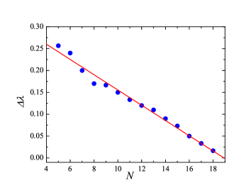
Figure 8: (Color online) Width of the coupling interval where OD occurs, $\Delta\lambda\equiv\lambda_{\max}-\lambda_{\min}$ (see the text), as a function of the number of rotators $N$ for $M=1,\delta=0.2,T=5.52,m_{j}=1-10^{-14}$. The line denotes the linear fit $\left(0.32988-0.01744N\right)$. The quantities plotted are dimensionless.

Figure 9: (Color online) Phase-space portraits of different periodic attractors corresponding to a starlike network [Eq. (1)] within a range of multistability for $N=10,M=1,\delta=0.2,T=5.52,\lambda=0.3$. (a) Hub ($m_{H}=0$, dotted line), single leaf subjected to control ($m_{1}=0.9$, solid line), and remaining leaves being fully synchronized ($m_{i}=0,i=2,...,9$, dashed line). (b) Antisymmetric versions of the attractors plotted in (a), respectively. (c) Hub ($m_{H}=0$, dotted line), single leaf subjected to control ($m_{1}=0.9$, solid line), and remaining leaves grouped into two clusters of distinct synchronized dynamics (dashed lines). (d) Antisymmetric versions of the attractors plotted in (c), respectively.

III.2 Control on an increasing number of peripheral rotators

It is interesting to study the accumulative effect of decreasing the pulses’ impulse on an increasing number of peripheral rotators $\left(M>1\right)$, while the hub remains subjected to trigonometric pulses, in the weak coupling regime where synchronization phenomena do not yet dominate the networks’ dynamics. We start from a situation where regularization is not possible for almost any value of the shape parameter when the pulses’ impulse is decreased on a single peripheral rotator ($M=1$, see Fig. 10(a)). Then, by increasing $M$ from unity, one typically obtains regularization of the whole network for sufficiently narrow pulses, on the one hand, and a deterioration of the synchronization of the chaotic dynamics for wider pulses on the other (see Fig. 10(b)). This further effect, which is especially noticeable when $M$ is near $N/2$ (compare the case $M=5$ with the cases $M=1$ and $M=7$, cf. Figs. 10(b), 10(a), 10(c), respectively), is due to the appearance of two different synchronized populations of rotators subjected respectively to pulses of different widths. As $M$ approximates $N-1$, i.e., when the impulse control is applied to all the peripheral rotators, the width of the interval $\Delta m$ where reshaping-induced regularization occurs increases, while the synchronization increases drastically even when the dynamics is chaotic, as for $M=9=N-1$ (see Fig. 10(d)).

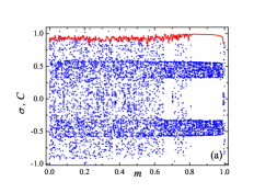
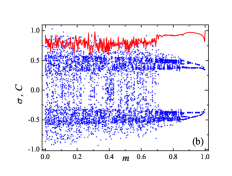
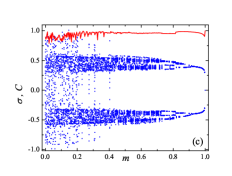
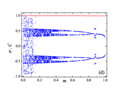
Figure 10: (Color online) Bifurcation diagrams of the average velocity $\sigma$ (blue (black) dots) and correlation function $C$ (red (gray) line) as a function of the shape parameter $m=m_{j}$ for the case of a central rotator subjected to trigonometric pulses $\left(m_{H}=0\right)$, $N=10,\lambda=0.1,\delta=0.2,T=5.52$, and four values of the number of peripheral rotators $x_{j}$ subjected to impulse control: (a) $M=1$, (b) $M=5$, (c) $M=7$, and (d) $M=9$. The quantities plotted are dimensionless.

III.3 Control on the central rotator

In the present subsection and the next, we study the role played by the degree of connectivity in the reshaping-induced chaos-control scenario by decreasing the pulses’ impulse on the central rotator. In the case of a single control (the present subsection), one finds that controlling the most highly connected rotator is by far the most effective control procedure (compare Fig. 11 with Fig. 10(a)). Strikingly, solely decreasing the impulse of the pulses acting on the hub $\left(M=0\right)$ is a much better choice than controlling even several peripheral rotators but not the hub, as in the case $M=5=N/2$ shown in Fig. 10(b). The reason for this relatively good effectiveness stems from two facts. First, solely controlling the hub does not significantly break the synchronization of the whole network when $N$ is sufficiently large (as for $N=10$, cf. Fig. 11). Second, its maximum degree of connectivity allows the hub to directly influence all the remaining (peripheral) rotators$-$in the sense of taming their chaotic dynamics$-$due to it is behaving as an energy sink for sufficiently narrow pulses, as seen in the energy analysis above (cf. Sec. II B).

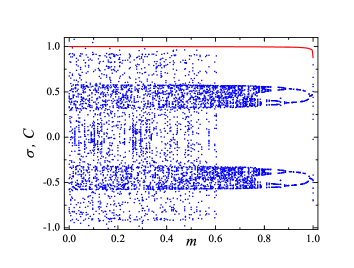
Figure 11: (Color online) Bifurcation diagrams of the average velocity $\sigma$ (blue (black) dots) and correlation function $C$ (red (gray) line) as a function of the shape parameter $m=m_{H}$ when the central rotator (hub) is the single rotator subjected to impulse control for $N=10,\lambda=0.1,\delta=0.2,T=5.52$. The quantities plotted are dimensionless.

III.4 Control on both the central and the peripheral rotators

Once the hub has been subjected to impulse control, one could expect a priori that additionally controlling other (peripheral) rotators should improve the network’s regularization. When the impulse transmitted by the control pulses is comparable to that transmitted by the trigonometric pulses (see Fig. 4), one typically finds the opposite effect however: a deterioration of the network’s regularization, as for the case $M=1$ (cf. Fig. 12(a)). This deterioration effect, which occurs together with increasing desynchronization, persists, and even increases, as the number of peripheral rotators subjected to control is increased, as for the case $M=5=N/2$ (cf. Fig. 12(b)) where desynchronization is maximum (compare Fig. 12(b) with Figs. 12(a) and 12(c) which correspond to the cases $M=1$ and $M=7$, respectively). As expected, when all rotators are subjected to the same impulse control, as for the case $M=9$ (cf. Fig. 12(d)), the network synchronization becomes perfect and the regularization route as the shape parameter is varied coincides with that of an isolated rotator subjected to the same remaining parameters, involving several consecutive crises followed by an inverse period doubling to finally reach the equilibrium $\left(x=0,\overset{.}{x}=0\right)$ when the common shape parameter is sufficiently near $1$.

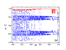
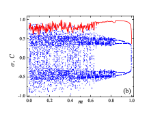
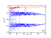
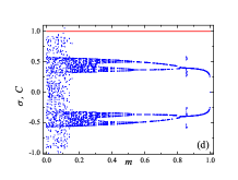
Figure 12: (Color online) Bifurcation diagrams of the average velocity $\sigma$ (blue (black) dots) and correlation function $C$ (red (gray) line) as a function of the shape parameter $m=m_{j}=m_{H}$ for the case of a central rotator subjected to impulse control, $N=10,\lambda=0.1,\delta=0.2,T=5.52$, and four values of the number of peripheral rotators $x_{j}$ subjected to impulse control: (a) $M=1$, (b) $M=5$, (c) $M=7$, and (d) $M=9$. The quantities plotted are dimensionless.

IV DISCUSSION

To summarize, we have demonstrated theoretically and numerically that the impulse transmitted by periodic pulses is a fundamental quantity for the reliable control of the chaotic behavior of starlike networks of damped kicked rotators. We have shown how the effectiveness of pulse reshaping, when it is applied to a single node, strongly depends upon the degree of the target node: applying impulse-decreasing pulses to the highest-degree node is by far the best suppressory strategy, while applying them to low-degree nodes is the poorest choice. In the case of applying pulse control to several nodes, we found rather counterintuitive results: more is not only different but often means poorer regularization. We have shown that this is due to desynchronization phenomena which result from the competition between two comparable populations of rotators subjected to pulses transmitting comparable but different impulses. When the pulses’ impulse is sufficiently small, the rotator subjected to control behaves as an energy sink for the remaining rotators, and this is ultimately the basic physical mechanism leading to the network’s regularization. Clearly, the effectiveness of this localized dissipation of energy strongly depends upon the target node’s degree, which explains why controlling the central node is a much better choice than controlling a peripheral node. The decreasing-impulse-induced chaos-control scenario discussed could find applications in diverse biological coupled systems [31], including neuronal networks [32]. It may also be useful to optimally control chaos in scale-free networks of dissipative periodically-kicked oscillators since a highly connected node in such a network can be thought of as a hub of a locally starlike part of the network, with a degree of connectivity that belongs to the complete network’s degree-of-connectivity distribution.

- (1) Y.-Y. Liu, J.-J. Slotine, and A.-L. Barabási, Nature 473, 167 (2011).
- (2) T. Nepusz and T. Vicsek, Nat. Phys. 8, 568 (2012).
- (3) M. Pósfai, Y.-Y. Liu, J.-J. Slotine, and A.-L. Barabási, Sci. Rep. 3, 1067 (2013).
- (4) S. P. Cornelius, W. L. Kath, and A. E. Motter, Nat. Commun. 4, 1942 (2013).
- (5) G. Menichetti, L. Dall’Asta, and G. Bianconi, Phys. Rev. Lett. 113, 078701 (2014).
- (6) R. Laje and D. V. Buonomano, Nat. Neurosci. 16, 925 (2013).
- (7) D. Delpini et al., Sci. Rep. 3, 1626 (2012).
- (8) G. Chen and X. Dong, From Chaos to Order (World Scientific, Singapore, 1998).
- (9) R. Chacón, Control of Homoclinic Chaos by Weak Periodic Perturbations (World Scientific, Singapore, 2005).
- (10) Handbook of Chaos Control, 2nd ed., edited by E. Schöll and H. G. Schuster (Wiley-VCH, Weinheim, 2008).
- (11) W. Wang, I. Z. Kiss, and J. L. Hudson, Phys. Rev. Lett. 86, 4954 (2001).
- (12) P. J. Martínez and R. Chacón, Phys. Rev. Lett. 93, 237006 (2004); 96, 059903(E) (2006).
- (13) K. Rajan, L. F. Abott, and H. Sompolinsky, Phys. Rev. E 82, 011903 (2010).
- (14) R. Albert and A.-L. Barabási, Rev. Mod. Phys. 74, 47 (2002).
- (15) L. M. Pecora, Phys. Rev. E 58, 347 (1998).
- (16) Z. Ma, G. Zhang, Y. Wang, and Z. Liu, J. Phys. A: Math. Theor. 41, 155101 (2008).
- (17) A. Bergner et al., Phys. Rev. E 85, 026208 (2012).
- (18) P. V. Kuptsov and A. V. Kuptsova, Phys. Rev. E 92, 042912 (2015).
- (19) D. A. Steck, W. H. Oskay, and M. G. Raizen, Science 293, 274 (2001).
- (20) R. Chacón, Phys. Rev. E 74, 046202 (2006).
- (21) R. Chacón and A. Martínez García-Hoz, Phys. Lett. A 281, 231 (2001).
- (22) R. Chacón and A. Martínez García-Hoz, Phys. Rev. E 68, 066217 (2003).
- (23) A. Koseska, E. Volkov, and J. Kurths, Phys. Rep. 531, 173 (2013).
- (24) V. K. Melnikov, Trans. Moscow Math. Soc. 12, 1 (1963) [Tr. Mosk. Ova. 12, 3 (1963)].
- (25) J. Guckenheimer and P. Holmes, Nonlinear Oscillations, Dynamical Systems, and Bifurcations of Vector Fields (Springer-Verlag, New York, 1983).
- (26) G. Benettin, L. Galgani, and J. M. Strelcyn, Phys. Rev. A 14, 2338 (1976); I. Shimada and T. Nagasama, Prog. Theor. Phys. 61, 1605 (1979).
- (27) I. S. Gradshteyn and I. M. Ryzhik, Table of Integrals, Series, and Products (Academic Press, San Diego, 1980).
- (28) J. V. Armitage and W. F. Eberlein, Elliptic Functions (Cambridge University Press, Cambridge, 2006).
- (29) See, e.g., S. H. Strogatz, Nonlinear Dynamics and Chaos (Addison-Wesley, Reading, MA, 1994), p. 249.
- (30) A. N. Pisarchik and U. Feudel, Phys. Rep. 540, 167 (2014).
- (31) E. Ullner, A. Zaikin, E. I. Volkov, and J. García-Ojalvo, Phys. Rev. Lett. 99, 148103 (2007).
- (32) S. J. Schiff, Neural Control Engineering (MIT Press, Cambridge, 2012).