Using Newton’s method to model a spatial light distribution of a LED with attached secondary optics

Abstract

In design of optical systems based on LED (Light emitting diode) technology, a crucial task is to handle the unstructured data describing properties of optical elements in standard formats. This leads to the problem of data fitting within an appropriate model. Newton’s method is used as an upgrade of previously developed most promising discrete optimization heuristics showing improvement of both performance and quality of solutions. Experiment also indicates that a combination of an algorithm that finds promising initial solutions as a preprocessor to Newton’s method may be a winning idea, at least on some datasets of instances.

Highlights:

• Model for data fitting of LED photometry with the evaluation function is presented.

• The effects of a numerical method in conjunction with heuristics are studied.

• Algorithms are developed with the use of C++ programing language.

• The success of developed algorithms is tested on real and artificial datasets.

• The results are statistically evaluated.

• The numerical Newton’s method prevails on both datasets, and provides substantial runtime shortening.

1 Introduction

The LED (Light emitting diode) industry has been evolving rapidly in the past several years. The fast pace of research and development in the field had some expected impact. One of the results is a massive use and implementation od LED elements in all kind of luminaires. While some of these luminaires are designed for ambient illumination the majority are technical luminaires that have to conform not only to electrical and mechanical safety regulations but also to regulations that define and restrict the photometry of a certain luminaire. This means that the photometry of a luminaire has to be defined prior to the production. In order to do that efficiently and with minimal errors the design engineer must virtually test the luminaires performance. Tools that can be used (OpticsWorks, LigthTools, TracePRO) [1, 2, 3] do exist and they offer a vast repository of sub-modules to develop and design custom lenses, reflectors, light guides, etc. These universal tools however do not completely exploit the luminaire design possibilities that were introduced by the transition from conventional light source technologies to LED. One of the possibilities which is also the main goal of a bigger study that incorporates the research presented here is to have an expert or intelligent system which would be capable of suggesting a secondary lens combination that would result in a user defined end photometry. In other words, the system would take some stock secondary LED lenses from different manufactures, place them on a defined LED array and search for the optimal combination of the lenses so that the resulting photometry would be as close as possible to the user defined one.

The method could enable the luminaire designer to custom design the light engine to a specific area of illumination, while keeping the mechanical and electrical parts of a luminaire untouched. This would in turn provide a customer with a tailored solution that would guarantee a maximum efficiency, lower prices, fewer light pollution and the possibility to individualize the illumination effect while maintaining a consistent visual appearance of the luminaries. There are several optimization tasks related to development of the above idea. Here we focus on the approximation of spatial light distribution with a moderate number of suitable basis functions [4, 5]. The problem that is defined formally in the next section is motivated by the following. The data describing the properties of the lenses and/or of the desired light distribution is nowadays usually given in some standard format files that correspond to the measured (or desired) values at a number of points in space. This results in relatively large data files of unstructured data. Clearly, if the data can be well enough approximated c.f. as a linear combination of certain basis functions, this may enable faster computations using less computer storage. Indeed, for some special cases including LED lenses with symmetric light distribution, it is possible to find reasonably good approximations fast (8 minutes runtime on a Intel Core I7-4790K CPU @ 4 Ghz, the code is written in C++ and is not fully optimized). Sufficiently good approximation here means 2-5% RMS error (to be defined later) for target light distribution, taking into account expected noise in measurement using current technology. Recent experiments showed that sufficiently good approximations can be obtained by some basic optimization algorithms, including local search algorithms and genetic algorithms [6, 7, 8]. However, when using predefined lenses to design a luminaire that closely approximates a desired light distribution, it may be essential that the approximation error is much lower.

The same task can also be seen as solving a problem of data compression, replacing a long unstructured data file with a much shorter one, in this case a sequence of parameters. It makes sense to aim at 0% approximation when considering the data compression task.

As the functions to be approximated are smooth, it is natural to try to improve the basic discrete optimization methods with continuous optimization techniques, c.f. Newton’s method [9]. Here we consider Newton’s method both as a standalone (restarted) algorithm and as a post-processor of other algorithms. The datasets used for testing and analysis are a selection of real lenses as used in previous studies and an artificial dataset that is large enough for statistical analysis. The artificial dataset is also generated in a way which assures that 0% approximation is possible. Note that we have no guarantee that the realistic lenses may be approximated within our model with arbitrary low RMS error. The rest of the paper is organized as follows. In section two we discus the problem and present the mathematical model, section three is all about the algorithms and Newton method implementation, section four presents the datasets used in the experiment, section five provides the experiment set-up, section six unveils the results section seven wraps everything up in the conclusion. Appendix provides all equations needed for the Newton method.

2 The model

The method mentioned above seems natural and straightforward, but at a closer look, we observe some fundamental problems related to realization of the main idea. Namely, both the spatial light distribution of LED lenses and the desired illumination are given in the standard data formats, that are just a long unstructured lists of data. In particular when the aim is to construct a lighting system that provides the desired illumination of the environment, it is necessary or at least very convenient to have the data in some more structured format. It is known that the spatial light distribution of some LED lenses can be approximated by a sum of a small number of certain basis functions [4]. Provided the approximation is sufficiently good, it may be possible to provide designs combining several lenses with controlled error rate.

This naturally opens several research avenues. For example, it is important to have error free or at least very good approximations of the basic lenses, and to have methods that are stable in the sense that they are not too sensitive to the noise in the presentation of basic elements.

Here we focus on the first above mentioned task, approximation of the unstructured spatial light distribution data. We search for an approximation of the Luminous intensity $I\left(\varPhi;\textbf{a},\textbf{b},\textbf{c}\right)$ at the polar angle of $\varPhi$ in the form

$$I\left(\varPhi;\textbf{a},\textbf{b},\textbf{c}\right)=I_{max}\sum_{k=1}^{K}\ a_{k}\cos^{c_{k}}(\varPhi-b_{k})$$ (1)

where $K$ is the number of functions to sum and $a_{k}$, $b_{k}$, $c_{k}$ are the function coefficients that we search for. For brevity, coefficients are written as vectors $\textbf{a}=(a_{1},a_{2},\dots,a_{K})$, $\textbf{b}=(b_{1},b_{2},\dots,b_{K})$, and $\textbf{c}=(c_{1},c_{2},\dots,c_{K})$. The interval range of the coefficients is: $a=[0,1]$, $b=[0,90]$ and $c=[0,100]$, more accurately the discrete values are : $a_{\star}\in[0,0.001,0.002,\dots,1]$, $b_{\star}\in[-90,-89.9,-89.8,\dots,90]$, and $c_{\star}\in[0,1,2,\dots,100]$. Here we need to note two restrictions on the model. First restriction emerges from the LEDs physical design. The LED can not emit any light to the back side which is the upper hemisphere in our case. That is why all intermediate values that are calculated at the combined angle $(\varPhi-b_{k})$ greater than 90° equal 0. The second restriction deals with the slightly unusual description of the light distribution in standard files such as Elumdat (file extension .ldt) [10] and Iesna (.ies) [11]. These files present measured candela values per angle $○\varPhi$ on so called C planes which can be observed on Figure 1. One C plane is actually only one half of the corresponding cross-section and does not describe the other half. But from a physical point of view we need to consider the impact from the other half of the cross-section. Because all the lenses used here are symmetric, we can simplify the calculation of the intermediate values and incorporate the impact of the other half by mirroring (multiplying by -1) all values that are calculated with the combined angle $(\varPhi-b_{k})$ less than 0°. Note however that this only works with symmetrical distributions, and should be reconsidered carefully when the method is to be applied to asymmetrical distributions.

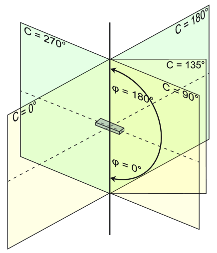
Figure 1: C-planes according to standard. C-planes angles : 0° - 360° — $\varPhi$ angles : 0° to 90°

The goodness of fit is defined as the root mean square error ($RMS$), formally defined by the expression:

$$RMS\left(\textbf{a},\textbf{b},\textbf{c}\right)=\sqrt{\frac{1}{N}\sum_{i=1}^{N}\left[I_{m}(\varPhi_{i})-I(\varPhi_{i},\textbf{a},\textbf{b},\textbf{c})\right]^{2}}$$ (2)

where $RMS$ represents the error of the approximation.Later in tables we provide the relative RMS error (RMSp) defined with equation 3. $N$ is the number of measured points in the input data, $I_{m}(\varPhi_{i})$ the measured Luminous intensity value at the polar angle $\varPhi$ from the input data, and $I(\varPhi_{i},\textbf{a},\textbf{b},\textbf{c})$ the calculated Luminous intensity value at the given polar angle $\varPhi$.

$$RMS_{p}\left(\textbf{a},\textbf{b},\textbf{c}\right)=\frac{100*N*RMS\left(\textbf{a},\textbf{b},\textbf{c}\right)}{\sum_{i=1}^{N}\left[I_{m}(\varPhi_{i})\right]}\left[\%\right]$$ (3)

Remark. The model was successfully applied to LED’s with attached secondary optics and symmetric light distribution [4] showing that sufficiently good approximations (RMS error below 5%) can be obtained using a sum of only three functions ($K=3$). Approximation of spatial light distribution of a LED with uniform distribution and without a secondary lens using this type of functions was first proposed in [5]. The model was slightly modified in [4] where a new normalizing parameter was introduced, and consequently, all other parameters will have values in fixed intervals known in advance. It should be noted that the modified model is equivalent to the original, only the number of parameters and their meaning differ. It may be interesting to note that due to symmetries of the examples, $K=3$ is sufficient for both applications [4, 5]. In general case, we expect that $K>3$ functions will be needed for sufficiently good approximations, and in view of optimization of the design of a luminaire it is interesting to have an idea how large the parameter $K$ can grow to assure that the light distribution fits the desired (and/or standard) sufficiently well. We do not address this question here.

When applying the model to the data compression problem, the target RMS error is 0%. Therefore, we aim to improve the approximation results that were obtained previously [6, 7] and restrict attention to symmetric light distributions. Also, we fix $K=3$ functions in the model. Besides the dataset of 14 realistic lenses that was used in some previous studies, here we also generate an artificial dataset in which a sample is simply a sum of three basis functions with randomly chosen parameters. This assures that zero error approximation is possible for the instances of the artificial dataset.

We are interested first in minimizing the approximation error, and second, in computational time of the methods. In the next section we briefly outline the algorithms we use in the experiments.

3 The algorithms

In previous work [6, 7], the model described above was applied in conjunction with several custom build algorithms that are based on local search heuristics and some meta-heuristics. The algorithms implemented include a steepest descend algorithm, two iterative improvement algorithms with different neighbourhoods and two genetic algorithms, a standard one and a hybrid one in which the best individuals of every generation are optimized with the iterative improvement algorithm. For more detailed description of the algorithms we refer to [6, 7]. The results of the experiments showed that all of the algorithms applied are capable of providing satisfactory results on all tested instances, and differed mainly in computational time needed. The average RMS values obtained on real lenses were around $RMS=2\%$. Hence, the results mentioned proved that the model is accurate and that sufficiently good approximations can be found with a variety of algorithms for sufficiently good description of lenses.

However, recall that the model can also be used for data compression task. Zero or very low RMS error is also essential in the foreseen application, in which the pre manufactured lenses are to be combined into a more complex luminaire with prescribed light distribution.

In the model we use a sum of functions that are smooth and hence the first and second derivatives can be calculated allowing application of continuous optimization methods in addition to the general discrete optimization meta-heuristics that were used before. We have chosen to use the Newton (also known as the Newton–Raphson) iterative method [9] to find the solution that we seek. It is well known that convergence of the Newton method largely depends on the initial solution. Therefore we have applied the method in two ways. First, we use the Newton method as an optimizer which will pinpoint the local minimum of the solutions found by heuristic algorithms. In a sense this implementation of the Newton method will be an extension of the discrete optimization algorithm, used to finalize the search to end in a local minimum. (Note that the local minima may be missed by the discrete optimization algorithms due to predefined length of the discrete moves.) Second, we use the Newton method as a standalone algorithm that will on initialization generate a number of random (initial) solutions that are uniformly scattered over the whole search space and then it will use the Newton method on a number of the best initial solutions to find the local minimums. Of course, for both implementations to be comparable the iteration count has to be controlled so that the overall maximum amount of computation time will be roughly the same.

Preprocessor multi-start IF. The multi-start iterative improvement with fixed neighbourhood (IF) algorithm [7, 8] first initializes several initial solutions. The initial solutions are randomly chosen from the whole search space. Each of the initial solutions is then optimized using the following steps. In the beginning the search step values (a step for a numerical differentiation) $da=0.01$, $db=1$, and $dc=\frac{I_{max}}{10}$ are initialized, giving the 512 neighbours of the initial solution: ($a_{1}\pm da,b_{1}\pm db,c_{1}\pm dc$, $a_{2}\pm da,b_{2}\pm db,c_{2}\pm dc$, $a_{3}\pm da,b_{3}\pm db,c_{3}\pm dc$). Then the algorithm randomly chooses a neighbour, and immediately moves to the neighbour if its RMS value is better than the current RMS value. If no better neighbour is found after 1000 trials, it is assumed that no better neighbour exists. In this case the algorithm morphs the neighbourhood by changing the step according to the formula $d_{i+1}=d_{i}+d_{0}$. More precisely, $da_{i+1}=da_{i}+da_{0}$ where $da_{0}$ is the initial step value. Analogously for $db$ and $dc$.

This is repeated until $i=10$. If there still is no better solution, the initial step value is multiplied by $0.9$ and the search resumes from the current solution with a finer initial step. The algorithm stops when the number of generated solutions reaches $T_{max}$.

Newton method. Newton’s method [9, 12, 13] is a well-known numerical optimization method that can provide very good results under certain assumptions on the evaluation function and on the initial solution. Newton’s method indirectly minimizes the evaluation function by looking for a solution of a system of nonlinear equations (first derivatives of the evaluation function). Newton’s method solves the system of nonlinear equations iteratively by approximating it with a system of linear equations in each step which produce the delta vector. The delta vector is a part of the iterative sheme $\textbf{x}_{k}^{i+1}=\textbf{x}_{k}^{i}-\textbf{d}_{k}^{i}$. Newton method converges when the delta vector vanishes, $d=0$. At this point the evaluation coefficients found are the local minimum. Details are given in the Appendix. An obvious assumption is that the evaluation function has to be a continuous non-linear function for which first and second order derivatives are defined. The initial solution has to be close enough to a local or global optimum, for Newton’s method to converge. Hence the method is very sensitive to the choice of the initial solution.

4 The datasets

The experimental study uses two batches of instances, a dataset of 14 instances that correspond to real LED lenses, and a dataset of artificial instances generated for purpose of this experiment. The artificial lenses are used to obtain more conclusive result on the statistical test, because a sample of 14 is rather small and may provide statistically insignificant results. The real lenses on the other hand show that the algorithms are useful in real life scenarios.

Real lenses. We have chosen 14 different symmetrical lenses which are meant to be used with a CREE XT-E series LED, from one of the world’s leading lens manufacturer LEDIL from Finland. We acquired the photometric data from LEDIL’s on-line catalogue [14] The data was provided in .ies format, which we then converted to a vector list which is more suitable to use in our algorithms. LEDIL measured the individual lenses with a 1° polar precision on four C panels. This means that from every .ies file we extracted 720 vectors. As the lenses are symmetric we only needed one C panel, and because we are only working on the lower half of the sphere (DLOR) we end up with 91 vectors (counting the 0° vector) on which we approximate the model.

Artificial lenses. In the dataset of 100 artificial examples, each element in the dataset was generated as follows.

A value from an interval was generated using uniform random distribution. (Intervals are $[0,1]$, $[0,90]$, or $[0,10]$, depending on the parameter. More precisely, the random generator chose one of the values from the finite sets: $a_{1},a_{2},a_{3}\in\{0,0.001,0.002,\dots,0.999,1\}$, $b_{1},b_{2},b_{3}\in\{0,0.01,0.02,$ $\dots,$ $90\}$ and $c_{1},c_{2},c_{3}\in\{0,0.1,0.2,$ $\dots,$ $10\}$.) Then the function values or candela values were computed for each polar angle $\varPhi\in\{0,1,2,\dots,89\}$. The candela values for polar angles $\varPhi\in\{90,91,92,\dots,180\}$ were set to 0. The data was then encoded into a .ies file structure, giving a datafile of the same format as the real lenses have. Note that the data generated assure that in each case zero RMS error approximation is possible within our model. Second, the dataset of 100 samples is sufficiently large for meaningful statistical analysis of experimental results.

5 The experiment setup

Before we go ahead and explain the experiment set-up, let us first remember the evaluation function that is the basis of the Newton method [9]. We already showed that the goodness of fit is measured with the $RMS$ value which is calculated from (2). From that we can define the evaluation function as:

$$E\left(\textbf{a},\textbf{b},\textbf{c}\right)=\frac{1}{N}\sum_{i=1}^{N}\left[I_{max}(a_{1}\cos^{c_{1}}(\varPhi-b_{1})+a_{2}\cos^{c_{2}}(\varPhi-b_{2})+a_{3}\cos^{c_{3}}(\varPhi-b_{3}))-I_{m}(\varPhi_{i})\right]^{2}$$ (4)

where $E$ represents the error to be minimized, $N$ the number of measured points in the input data, $I_{max}$ the maximum candela value, $I_{m}(\varPhi_{i})$ the measured Luminous intensity value at the polar angle $\varPhi$ from the input data, and $I(\varPhi_{i})$ the calculated Luminous intensity value at the given polar angle $\varPhi$.

The experiment was set-up to provide data from different algorithms. This in turn enables an objective comparison and a statistical test to determine the best algorithm. Recall that we implemented the Newton method in two distinct ways. The first implementation uses the multi-start version of iterative improvement (IF) to find a good approximation which is then optimized via the Newton method. The second implementation uses the random generator to generate initial solutions of which 100 best are optimized with the Newton method. Table belowshows different algorithms that were prepared for the experiment.

Table 1: Experiment algorithms.

Config.	Algorithm	Multi-start	IF steps
Short runs 1 million
1	S-Newton	1000000	NA
3	IF10	10	100000
4	IF20	20	50000
5	IF50	50	20000
6	IF100	100	10000
Long runs 4 million
2	L-Newton	4000000	NA
7	IF40	40	100000
8	IF80	80	50000
9	IF200	200	20000
10	IF400	400	10000

Time. We ran the algorithms in two different lengths. The short run evaluates approximately one million possible solutions per instance (lens) in just under 45s, and the long run approximately four million possible solutions per instance in about 3 minutes on a Core I7 - 4790K CPU. Newton’s method took in average 3 to 4 iterations to converge which means that the time it took to run the Newton’s method is negligible in contrast to the time the whole algorithm run. Expressed in seconds, the Newton’s method took approximately $2*10^{-3}s$, opposed to minutes CPU for the heuristics. In addition to the different time/iteration spans we ran the algorithms on two instance sets.

Datasets. Recall the two datasets of instances explained above, the dataset of 14 real lenses and a the dataset of 100 randomly generated artificial instances.

Algorithms. We apply the Newton method both as a standalone algorithm (restarted on randomly generated initial solutions) and as a final step after discrete local search algorithm (IF) outlined above. There are several algorithms that vary in the number of multi-starts (or, equivalently in the length of each local search). Depending on the length (short run, long run) and the number of restarts we denote the algorithms by IF10, IF20, IF50, IF100 and by IF40, IF80, IF200, IF400. The versions without local search are denoted by S-Newton and L-Newton for short and long runs, respectively. See Table 1.

6 Experimental results

We will begin the section with a comparison of the raw experimental data followed by the performance (quality of results) ranking and finish with the results of the Wilcoxon Signed rank test.

Table 2: Artificial lenses statistical data in RMSp for short and long runs. Best two results are emphasized.

Algorithm	Mean	Std. dev.	Min.	Max.
Short runs 1 million
S-Newton	1.3797E-04	8.5102E-05	3.5054E-05	3.9148E-04
IF 10	2.3393E+01	3.0447E+01	5.8079E-05	2.4287E+02
IF 20	1.1211E+01	1.6382E+01	4.9583E-05	1.3287E+02
IF 50	6.3340E+00	9.2152E+00	4.1291E-05	6.8720E+01
IF 100	7.2277E-01	2.7120E+00	3.4934E-05	1.9051E+01
Long runs 4 million
L-Newton	1.3797E-04	8.5102E-05	3.5054E-05	3.9148E-04
IF 40	1.2085E+01	2.5447E+01	4.8905E-05	2.4287E+02
IF 80	1.7490E+00	4.2982E+00	3.5054E-05	1.9504E+01
IF 200	4.0423E-01	1.9606E+00	3.5054E-05	1.4237E+01
FI 400	6.1717E-01	2.4068E+00	3.4934E-05	1.8938E+01

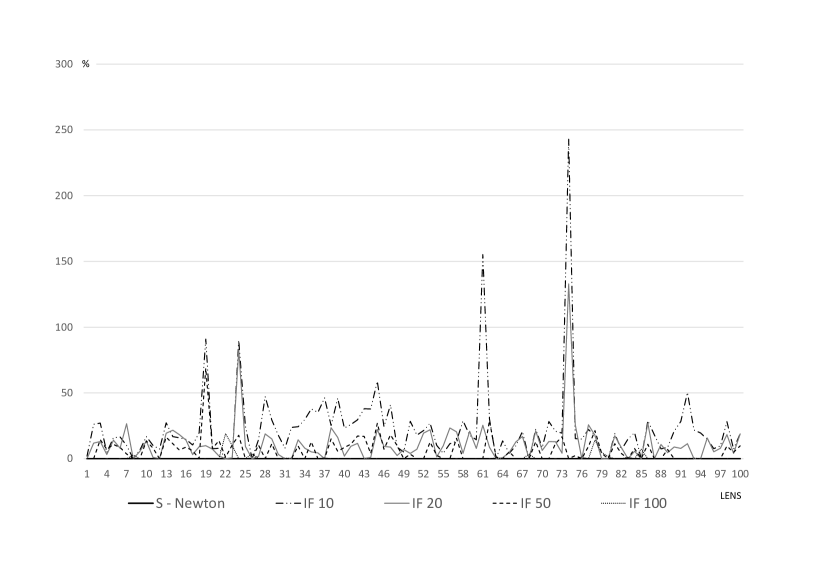
Figure 2: Best found solution on a short run. Artificial lenses per algorithm.

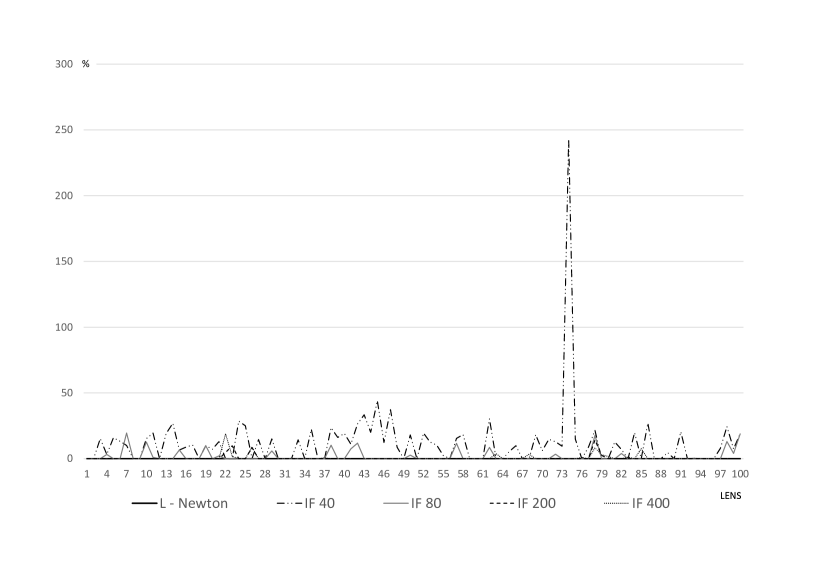
Figure 3: Best found solution on a long run. Artificial lenses per algorithm.

Table 3: Real lenses statistical data in RMSp for short and long runs.

Algorithm	Mean	Std. dev.	Min.	Max.
Short runs 1 million
S-Newton	5.3910E+00	3.7429E+00	1.7935E+00	1.5780E+01
IF 10	1.8657E+01	1.1726E+01	2.0361E+00	3.9179E+01
IF 20	5.4893E+00	2.9982E+00	1.4134E+00	1.0765E+01
IF 50	5.2665E+00	3.1108E+00	1.1120E+00	1.0768E+01
IF 100	4.8658E+00	2.6844E+00	1.1081E+00	1.0781E+01
Long runs 4 million
L-Newton	4.6116E+00	2.6540E+00	1.1254E+00	1.0327E+01
IF 40	1.8218E+01	1.1024E+01	6.3836E+00	3.9179E+01
IF 80	5.5141E+00	2.9581E+00	1.7265E+00	1.0764E+01
IF 200	5.2529E+00	2.9357E+00	1.9582E+00	1.0766E+01
FI 400	4.9059E+00	2.6582E+00	1.3586E+00	1.0786E+01

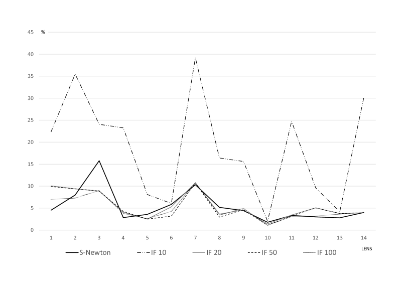
Figure 4: Best found solution on a short run. Real lenses per algorithm.

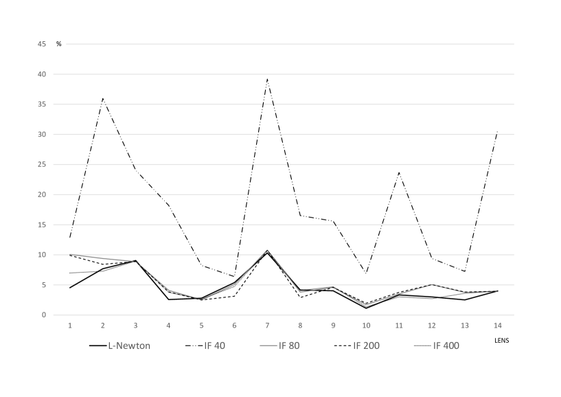
Figure 5: Best found solution on a long run. Real lenses per algorithm.

Experimetal results are given in Figures 2, 3, 4, 5 and are summarized in Table 2 and Table 3.

Comparison of the algorithms based on raw experimental results. Obviously, the pure multi-start Newton method is by far the best on artificial instances.

On the real lenses, the situation is a bit different. The Iterative improvement on several occasions outperforms the Newton method with random initial solutions. On both datasets, the long run yields only slightly better results as the short run does (and the short run is four times faster in executing). While we have no idea how far from optimal solutions the achieved values are for real lenses, we know that, by construction, a solution with 0% RMS error exists for each of the artificial lenses. Because of that it is worth to note that on the artificial set, the random algorithms found nearly optimal solutions in all cases. The RMS errors are in the range of E-04, which still is not pure 0% RMS error, but the very small difference could be due to rounding of the values in the .ies files.

On the other hand we did not find very low RMS values on the real set. The values that were found corresponded with the values of previous test that were performed without any numerical assistance. We did however perform an experiment on the real set with longer running time, in which we generated 16 million and 64 million initial solutions that showed similar behaviour. The mean error and the minimum error over 14 lenses decreased under 3.0% and 1.50% with 16 million generated solutions, and under 2.0% and 1.0% RMS error after 64 million.

While the success of the Newton method on artificial lenses is not surprising, it is not clear why the method is struggling on the realistic dataset. The winners in this comparison are on both sets the same, but on the real set the differences between the random Newton and IF assisted Newton algorithms are a lot smaller than on the artificial set, we even see that on some instances the IF algorithms are better. This could be due to the fact that IF algorithm was previously developed for real lenses that are from a limited range in search space and thus has a slight advantage on the set. The advantage of the pure Newton method on the artificial dataset can nicely be observed from the data scatter in Figure 6. We see that the IF algorithms provide very high degree of data scatter where the random ones provide very narrow result window. This may be due to the nature of the search because the IF algorithms focus in one defined direction which may not be the best one. Because of that the Newton optimization can not escape the potential pitfall of the direction. In contrast, the randomly generated solutions generally find lower quality results that at the same time provide more maneuvering space for the Newton method to find the best direction on more takes.

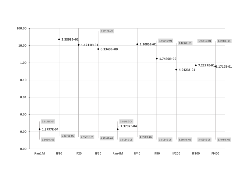
Figure 6: Min-Max scatter diagram for artificial lenses. Logarithmic y axis!

A comparison of the algorithms based on weighted ranking.

We assign a weight from 1 to 10 to each instance solution per algorithm. If the algorithm found the best solution on an instance it would get the weight 10 and if it found the second best solution it would get the weight 9, and so on until 1 for the worst solution. The total score of the algorithm is the sum of the scores on each instance.

In the same way, we compute the score based on the average values per algorithm and lens. The results are presented in Table 4.

Table 4: Weight based ranking.

R A N K
	Artificial				Real
	Best		Mean		Best		Mean
	Alg.	Score	Alg.	Score	Alg.	Score	Alg.	Score
1	L-Newton	944	L-Newton	1000	L-Newton	102	L-Newton	140
2	S-Newton	940	S-Newton	900	IF 100	97	S-Newton	124
3	IF 200	836	IF 20	588	IF 400	96	IF 10	114
4	IF 80	810	IF 100	585	IF 50	94	IF 50	89
5	IF 100	678	IF 10	559	S-Newton	90	IF 20	77
6	IF 400	660	IF 50	538	IF 20	88	IF 100	72
7	IF 50	529	IF 400	385	IF 200	86	IF 40	61
8	IF 40	514	IF 40	358	IF 80	83	IF 80	39
9	IF 20	379	IF 80	304	IF 10	23	IF 400	34
10	IF 10	212	IF 200	283	IF 40	21	IF 200	20

Note that the ranking here compares both short and long runs. As expected, Table 4 confirms the superiority of the pure Newton method on the artificial dataset. However, the situation is much more complicated on the dataset of real lenses. Despite the Newton method (long and short run) being the two best when considering the average results, they are not both when looking at the best solutions! The long run Newton is still the overall best, but the short run Newton is on the fifth place outran by two short IF algorithms and one long IF algorithm. We can also observe that the score differences are much smaller on the real set, which indicates that the pure Newton method is not as superior as it was on the artificial set. The lesser superiority could be explained in part by fact that the IF algorithms were developed using the real lens set. Hence the IF could have some unexpected advantages. However the Newton method improves the results in all cases.

Wilcoxon test. The third comparison is based on the statistical paired singed Wilcoxon [15] rank test. The statistical test compares algorithms pair by pair to estimate the difference between them. This is done via the asymptotic difference. If the value of the asymptotic difference is lower than $0.05$ then the algorithms in pair significantly differ one from another. The asymptotic differences of algorithm pairs will be presented in tables 5,6,7, and 8.

Table 5: Asymptotic significances of Wilcoxon Signed rank test for results for short runs on artificial lenses.

ALG	IF 20	IF 50	IF 100	S-Newton
IF 10	4.078E-11	1.020E-13	1.000E-13	1.000E-13
IF 20		7.162E-04	3.120E-13	1.000E-13
IF 50			3.628E-06	1.650E-13
IF 100				3.234E-08

Table 6: Asymptotic significances of Wilcoxon Signed rank test for results for long runs on artificial lenses.

ALG	IF 80	IF 200	IF 400	L-Newton
IF 40	1.736E-11	3.917E-11	7.950E-09	1.899E-12
IF 80		3.269E-11	5.563E-01	3.411E-06
IF 200			4.818E-06	7.044E-05
IF 400				1.176E-08

Table 7: Asymptotic significances of Wilcoxon Signed rank test for results for short runs on real lenses.

ALG	IF 20	IF 50	IF 100	S-Newton
IF 10	9.815E-04	9.815E-04	9.815E-04	9.815E-04
IF 20		4.326E-01	4.133E-02	5.936E-01
IF 50			5.098E-01	9.750E-01
IF 100				4.703E-01

Table 8: Asymptotic significances of Wilcoxon Signed rank test for results for long runs on real lenses.

ALG	IF 80	IF 200	IF 400	L-Newton
IF 40	9.815E-04	9.815E-04	9.815E-04	9.815E-04
IF 80		5.509E-01	5.553E-02	3.546E-02
IF 200			4.703E-01	1.240E-01
IF 400				4.703E-01

A look over the Wilcoxon test results reveals that there mostly are no similarities between algorithms when they ran on the artificial set. We can see that the Asymptotic significance values are very low, which means that there are significant differences between algorithms in pairs. We do however have one exception that is the pair IF 80 - IF 400, where the asymptotic difference is just over the margin, so we could say that these two have some similarities. The story is completely different on the real dataset, where we can find that most IF algorithms are similar to random algorithms. This also corresponds with the findings of the ranking and RMS error comparison. The Wilcoxon test provided similar conclusions as the previous tests did, but we need to be careful because the data sets differ in size and the real lenses set can be a bit inconclusive as it is a rather small sample with only 14 instances. That is why the artificial lenses with 100 instances could give a more accurate result.

Table 9: . Real lens RMSp for RAN 4M with and without Newton’s method. Quality increase $\Delta$ in %.

Instance	RAN 4M	Newton	$\Delta$
CP12632	27,996	7,6908	72,53
CP12634	45,8986	9,05513	80,27
CP12633	10,7706	2,57185	76,12
CA11934	10,2492	2,7982	72,70
CA11268	15,1818	5,38851	64,51
CP12817	29,6252	10,3279	65,14
CA11265	9,64366	4,1553	56,91
CP12636	7,62895	4,03813	47,07
CA13013	2,70647	1,12548	58,42
FP13030	10,1866	3,34882	67,13
CA11525	12,0224	3,00557	75,00
CA12392	6,87747	2,51916	63,37
CA11483	24,5813	4,0032	83,71

7 Conclusion

Here we presented an upgrade of a previously developed most promising discrete optimization heuristics with a numerical approach to optimization. It was shown that application of Newton’s method gave improvement of both performance and quality of solutions. In terms of raw performance, we got from the initial 8 minutes’ runtime for one algorithm on one lens to about 45s runtime with the upgraded IF 10 or S-Newton algorithm. The stated runtime is accurate for symmetric lenses and an input of 91 vectors. When working on asymmetric lenses the input will be around 33.000 vectors, this is when the problem becomes a big data problem. But because of the algorithms construction the runtime should increase to about 2 hours and 15 minutes. The increase will be by a factor of 180, while the amount of vectors is increased by a factor 360. On the asymmetric lenses the runtime will be lowered from around 24 hours to 2 hours and 15 minutes. Despite the drastic time shortening the quality of the solutions was not worse thanks to Newton’s method, which enabled us to find local minimums on the majority of solutions found by the heuristic algorithms. Newton’s method in fact successfully minimized the RMS error on all of the experiment cases with the average of 60% increased quality (minimized RMS) over previous experiments done in [4, 7]. This can be well observed in Table 9, where we can see the RMS error found by the RAN 4M algorithm before the application of Newton’s method and after. We can conclude that the integration of numerical approach with previously developed heuristics significantly improved the application performance to the level at which it is useful in the main research. On the other hand, we have learned that due to sensitiveness of Newton’s method to the choice of initial solutions, it may be rewarding to use a preprocessor that may provide promising initial solutions. In particular, on the dataset consisting of real lenses, the experiment showed that the initial solutions provided by a discrete local search algorithm improved the overall performance of the algorithm. This leads to the conclusion that a combination of an algorithm that finds promising initial solutions as a preprocessor to Newton’s method may be a winning combination, at least on some datasets of instances. Hence, in a practical application, it may be worth developing good heuristics that may handle specific properties of the instances and thus provide promising initial solutions for final optimization.

8 Acknowledgement

This work was supported in part by ARRS, the Research agency of Slovenia, grants P1-0285 and ARRS-1000-15-0510. We sincerely thank both reviewers for carefully reading the manuscript and for constructive remarks.

References

Appendix A

Evaluation function :

$$E\left(\textbf{a},\textbf{b},\textbf{c}\right)=\frac{1}{N}\sum_{i=1}^{N}\left[I_{max}(a_{1}\cos^{c_{1}}(\varPhi_{i}-b_{1})+a_{2}\cos^{c_{2}}(\varPhi_{i}-b_{2})+a_{3}\cos^{c_{3}}(\varPhi_{i}-b_{3}))-I_{m}(\varPhi_{i})\right]^{2}$$ (5)

Partial equations:

$$G_{i}=I_{max}(a_{1}\cos^{c_{1}}(\varPhi_{i}-b_{1})+a_{2}\cos^{c_{2}}(\varPhi_{i}-b_{2})+a_{3}\cos^{c_{3}}(\varPhi_{i}-b_{3}))-I_{m}(\varPhi_{i})$$ (6)

$$F_{1_{i}}=I_{max}\cos^{c_{1}}(\varPhi_{i}-b_{1})$$ (7)

$$F_{2_{i}}=I_{max}\cos^{c_{2}}(\varPhi_{i}-b_{2})$$ (8)

$$F_{3_{i}}=I_{max}\cos^{c_{3}}(\varPhi_{i}-b_{3})$$ (9)

$$F_{4_{i}}=I_{max}a_{1}c_{1}\cos^{(c_{1}-1)}(\varPhi_{i}-b_{1})\sin(\varPhi_{i}-b_{1})$$ (10)

$$F_{5_{i}}=I_{max}a_{2}c_{2}\cos^{(c_{2}-1)}(\varPhi_{i}-b_{2})\sin(\varPhi_{i}-b_{2})$$ (11)

$$F_{6_{i}}=I_{max}a_{3}c_{3}\cos^{(c_{3}-1)}(\varPhi_{i}-b_{3})\sin(\varPhi_{i}-b_{3})$$ (12)

$$F_{7_{i}}=I_{max}a_{1}\cos^{c_{1}}(\varPhi_{i}-b_{1})\ln(\cos(\varPhi_{i}-b_{1}))$$ (13)

$$F_{8_{i}}=I_{max}a_{2}\cos^{c_{2}}(\varPhi_{i}-b_{2})\ln(\cos(\varPhi_{i}-b_{2}))$$ (14)

$$F_{9_{i}}=I_{max}a_{3}\cos^{c_{3}}(\varPhi_{i}-b_{3})\ln(\cos(\varPhi_{i}-b_{3}))$$ (15)

$$S_{14_{i}}=I_{max}c_{1}\cos^{(c_{1}-1)}(\varPhi_{i}-b_{1})\sin(\varPhi_{i}-b_{1})$$ (16)

$$S_{17_{i}}=I_{max}\cos^{c_{1}}(\varPhi_{i}-b_{1})\ln(\cos(\varPhi_{i}-b_{1}))$$ (17)

$$S_{25_{i}}=I_{max}c_{2}\cos^{(c_{2}-1)}(\varPhi_{i}-b_{2})\sin(\varPhi_{i}-b_{2})$$ (18)

$$S_{28_{i}}=I_{max}\cos^{c_{2}}(\varPhi_{i}-b_{2})\ln(\cos(\varPhi_{i}-b_{2}))$$ (19)

$$S_{36_{i}}=I_{max}c_{3}\cos^{(c_{3}-1)}(\varPhi_{i}-b_{3})\sin(\varPhi_{i}-b_{3})$$ (20)

$$S_{39_{i}}=I_{max}\cos^{c_{3}}(\varPhi_{i}-b_{3})\ln(\cos(\varPhi_{i}-b_{3}))$$ (21)

$$S_{41_{i}}=I_{max}c_{1}\cos^{(c_{1}-1)}(\varPhi_{i}-b_{1})\sin(\varPhi_{i}-b_{1}))$$ (22)

$$S_{44_{i}}=I_{max}a_{1}c_{1}\cos^{(c_{1}-2)}(\varPhi_{i}-b_{1})(c_{1}\sin^{2}(\varPhi_{i}-b_{1})-1)$$ (23)

$$S_{47_{i}}=-I_{max}a_{1}\cos^{(c_{1}-1)}(\varPhi_{i}-b_{1})\sin(\varPhi_{i}-b_{1})(c_{1}\ln(\cos(\varPhi_{i}-b_{1}))+1)$$ (24)

$$S_{52_{i}}=I_{max}c_{2}\cos^{(c_{2}-1)}(\varPhi_{i}-b_{2})\sin(\varPhi_{i}-b_{2}))$$ (25)

$$S_{55_{i}}=I_{max}a_{2}c_{2}\cos^{(c_{2}-2)}(\varPhi_{i}-b_{2})(c_{2}\sin^{2}(\varPhi_{i}-b_{2})-1)$$ (26)

$$S_{58_{i}}=-I_{max}a_{2}\cos^{(c_{2}-1)}(\varPhi_{i}-b_{2})\sin(\varPhi_{i}-b_{2})(c_{2}\ln(\cos(\varPhi_{i}-b_{2}))+1)$$ (27)

$$S_{63_{i}}=I_{max}c_{3}\cos^{(c_{3}-1)}(\varPhi_{i}-b_{3})\sin(\varPhi_{i}-b_{3}))$$ (28)

$$S_{66_{i}}=I_{max}a_{3}c_{3}\cos^{(c_{3}-2)}(\varPhi_{i}-b_{3})(c_{3}\sin^{2}(\varPhi_{i}-b_{3})-1)$$ (29)

$$S_{69_{i}}=-I_{max}a_{3}\cos^{(c_{3}-1)}(\varPhi_{i}-b_{3})\sin(\varPhi_{i}-b_{3})(c_{3}\ln(\cos(\varPhi_{i}-b_{3}))+1)$$ (30)

$$S_{71_{i}}=I_{max}\cos^{c_{1}}(\varPhi_{i}-b_{1})\ln(\cos(\varPhi_{i}-b_{1}))$$ (31)

$$S_{74_{i}}=-I_{max}(a_{1}\cos^{c_{1}-1}(\varPhi_{i}-b_{1})\sin(\varPhi_{i}-b_{1})-a_{1}c_{1}\ln(\cos(\varPhi_{i}-b_{1}))\cos^{c_{1}-1}(\varPhi_{i}-b_{1})\sin(\varPhi_{i}-b_{1}))$$ (32)

$$S_{77_{i}}=I_{max}a_{1}\cos^{c_{1}}(\varPhi_{i}-b_{1})\ln(\cos(\varPhi_{i}-b_{1}))\ln(\cos(\varPhi_{i}-b_{1}))$$ (33)

$$S_{82_{i}}=I_{max}\cos^{c_{2}}(\varPhi_{i}-b_{2})\ln(\cos(\varPhi_{i}-b_{2}))$$ (34)

$$S_{85_{i}}=-I_{max}(a_{2}\cos^{c_{2}-1}(\varPhi_{i}-b_{2})\sin(\varPhi_{i}-b_{2})-a_{2}c_{2}\ln(\cos(\varPhi_{i}-b_{2}))\cos^{c_{2}-1}(\varPhi_{i}-b_{2})\sin(\varPhi_{i}-b_{2}))$$ (35)

$$S_{88_{i}}=I_{max}a_{2}\cos^{c_{2}}(\varPhi_{i}-b_{2})\ln(\cos(\varPhi_{i}-b_{2}))\ln(\cos(\varPhi_{i}-b_{2}))$$ (36)

$$S_{93_{i}}=I_{max}\cos^{c_{3}}(\varPhi_{i}-b_{3})\ln(\cos(\varPhi_{i}-b_{3}))$$ (37)

$$S_{96_{i}}=-I_{max}(a_{3}\cos^{c_{3}-1}(\varPhi_{i}-b_{3})\sin(\varPhi_{i}-b_{3})-a_{3}c_{3}\ln(\cos(\varPhi_{i}-b_{3}))\cos^{c_{3}-1}(\varPhi_{i}-b_{3})\sin(\varPhi_{i}-b_{3}))$$ (38)

$$S_{99_{i}}=I_{max}a_{3}\cos^{c_{3}}(\varPhi_{i}-b_{3})\ln(\cos(\varPhi_{i}-b_{3}))\ln(\cos(\varPhi_{i}-b_{3}))$$ (39)

First order derivatives:

$$\frac{\partial E(\textbf{a},\textbf{b},\textbf{c})}{\partial a_{1}}=\sum_{i=1}^{N}G_{i}F_{1_{i}}\qquad\frac{\partial E(\textbf{a},\textbf{b},\textbf{c})}{\partial a_{2}}=\sum_{i=1}^{N}G_{i}F_{2_{i}}$$

$$\frac{\partial E(\textbf{a},\textbf{b},\textbf{c})}{\partial a_{3}}=\sum_{i=1}^{N}G_{i}F_{3_{i}}\qquad\frac{\partial E(\textbf{a},\textbf{b},\textbf{c})}{\partial b_{1}}=\sum_{i=1}^{N}G_{i}F_{4_{i}}$$

$$\frac{\partial E(\textbf{a},\textbf{b},\textbf{c})}{\partial b_{2}}=\sum_{i=1}^{N}G_{i}F_{5_{i}}\qquad\frac{\partial E(\textbf{a},\textbf{b},\textbf{c})}{\partial b_{3}}=\sum_{i=1}^{N}G_{i}F_{6_{i}}$$ (40)

$$\frac{\partial E(\textbf{a},\textbf{b},\textbf{c})}{\partial c_{1}}=\sum_{i=1}^{N}G_{i}F_{7_{i}}\qquad\frac{\partial E(\textbf{a},\textbf{b},\textbf{c})}{\partial c_{2}}=\sum_{i=1}^{N}G_{i}F_{8_{i}}$$

$$\frac{\partial E(\textbf{a},\textbf{b},\textbf{c})}{\partial c_{3}}=\sum_{i=1}^{N}G_{i}F_{9_{i}}$$

Second order derivatives:

$$\frac{\partial^{2}E(\textbf{a},\textbf{b},\textbf{c})}{\partial a_{1}^{2}}=\sum_{i=1}^{N}F_{1_{i}}F_{1_{i}}\qquad\frac{\partial^{2}E(\textbf{a},\textbf{b},\textbf{c})}{\partial a_{2}\partial a_{1}}=\sum_{i=1}^{N}F_{1_{i}}F_{2_{i}}$$

$$\frac{\partial^{2}E(\textbf{a},\textbf{b},\textbf{c})}{\partial a_{3}\partial a_{1}}=\sum_{i=1}^{N}F_{1_{i}}F_{3_{i}}\qquad\frac{\partial^{2}E(\textbf{a},\textbf{b},\textbf{c})}{\partial b_{1}\partial a_{1}}=\sum_{i=1}^{N}F_{1_{i}}F_{4_{i}}+G_{i}S_{14_{i}}$$

$$\frac{\partial^{2}E(\textbf{a},\textbf{b},\textbf{c})}{\partial b_{2}\partial a_{1}}=\sum_{i=1}^{N}F_{1_{i}}F_{5_{i}}\qquad\frac{\partial^{2}E(\textbf{a},\textbf{b},\textbf{c})}{\partial b_{3}\partial a_{1}}=\sum_{i=1}^{N}F_{1_{i}}F_{6_{i}}$$

$$\frac{\partial^{2}E(\textbf{a},\textbf{b},\textbf{c})}{\partial c_{1}\partial a_{1}}=\sum_{i=1}^{N}F_{1_{i}}F_{7_{i}}+G_{i}S_{17_{i}}\qquad\frac{\partial^{2}E(\textbf{a},\textbf{b},\textbf{c})}{\partial c_{2}\partial a_{1}}=\sum_{i=1}^{N}F_{1_{i}}F_{8_{i}}$$

$$\frac{\partial^{2}E(\textbf{a},\textbf{b},\textbf{c})}{\partial c_{3}\partial a_{1}}=\sum_{i=1}^{N}F_{1_{i}}F_{9_{i}}$$

$$\frac{\partial^{2}E(\textbf{a},\textbf{b},\textbf{c})}{\partial a_{1}\partial a_{2}}=\sum_{i=1}^{N}F_{2_{i}}F_{1_{i}}\qquad\frac{\partial^{2}E(\textbf{a},\textbf{b},\textbf{c})}{\partial a_{2}^{2}}=\sum_{i=1}^{N}F_{2_{i}}F_{2_{i}}$$

$$\frac{\partial^{2}E(\textbf{a},\textbf{b},\textbf{c})}{\partial a_{3}\partial a_{2}}=\sum_{i=1}^{N}F_{2_{i}}F_{3_{i}}\qquad\frac{\partial^{2}E(\textbf{a},\textbf{b},\textbf{c})}{\partial b_{1}\partial a_{2}}=\sum_{i=1}^{N}F_{2_{i}}F_{4_{i}}$$

$$\frac{\partial^{2}E(\textbf{a},\textbf{b},\textbf{c})}{\partial b_{2}\partial a_{2}}=\sum_{i=1}^{N}F_{2_{i}}F_{5_{i}}+G_{i}S_{25_{i}}\qquad\frac{\partial^{2}E(\textbf{a},\textbf{b},\textbf{c})}{\partial b_{3}\partial a_{2}}=\sum_{i=1}^{N}F_{2_{i}}F_{6_{i}}$$

$$\frac{\partial^{2}E(\textbf{a},\textbf{b},\textbf{c})}{\partial c_{1}\partial a_{2}}=\sum_{i=1}^{N}F_{2_{i}}F_{7_{i}}\qquad\frac{\partial^{2}E(\textbf{a},\textbf{b},\textbf{c})}{\partial c_{2}\partial a_{2}}=\sum_{i=1}^{N}F_{2_{i}}F_{8_{i}}+G_{i}S_{28_{i}}$$

$$\frac{\partial^{2}E(\textbf{a},\textbf{b},\textbf{c})}{\partial c_{3}\partial a_{2}}=\sum_{i=1}^{N}F_{2_{i}}F_{9_{i}}$$

$$\frac{\partial^{2}E(\textbf{a},\textbf{b},\textbf{c})}{\partial a_{1}\partial a_{3}}=\sum_{i=1}^{N}F_{3_{i}}F_{1_{i}}\qquad\frac{\partial^{2}E(\textbf{a},\textbf{b},\textbf{c})}{\partial a_{2}\partial a_{3}}=\sum_{i=1}^{N}F_{3_{i}}F_{2_{i}}$$

$$\frac{\partial^{2}E(\textbf{a},\textbf{b},\textbf{c})}{\partial a_{3}^{2}}=\sum_{i=1}^{N}F_{3_{i}}F_{3_{i}}\qquad\frac{\partial^{2}E(\textbf{a},\textbf{b},\textbf{c})}{\partial b_{1}\partial a_{3}}=\sum_{i=1}^{N}F_{3_{i}}F_{4_{i}}$$

$$\frac{\partial^{2}E(\textbf{a},\textbf{b},\textbf{c})}{\partial b_{2}\partial a_{3}}=\sum_{i=1}^{N}F_{3_{i}}F_{5_{i}}\qquad\frac{\partial^{2}E(\textbf{a},\textbf{b},\textbf{c})}{\partial b_{3}\partial a_{3}}=\sum_{i=1}^{N}F_{3_{i}}F_{6_{i}}+G_{i}S_{35_{i}}$$

$$\frac{\partial^{2}E(\textbf{a},\textbf{b},\textbf{c})}{\partial c_{1}\partial a_{3}}=\sum_{i=1}^{N}F_{3_{i}}F_{7_{i}}\qquad\frac{\partial^{2}E(\textbf{a},\textbf{b},\textbf{c})}{\partial c_{2}\partial a_{3}}=\sum_{i=1}^{N}F_{3_{i}}F_{8_{i}}$$

$$\frac{\partial^{2}E(\textbf{a},\textbf{b},\textbf{c})}{\partial c_{3}\partial a_{3}}=\sum_{i=1}^{N}F_{3_{i}}F_{9_{i}}+G_{i}S_{39_{i}}$$

$$\frac{\partial^{2}E(\textbf{a},\textbf{b},\textbf{c})}{\partial a_{1}\partial b_{1}}=\sum_{i=1}^{N}F_{4_{i}}F_{1_{i}}+GS_{41_{i}}\qquad\frac{\partial^{2}E(\textbf{a},\textbf{b},\textbf{c})}{\partial a_{2}\partial b_{1}}=\sum_{i=1}^{N}F_{4_{i}}F_{2_{i}}$$

$$\frac{\partial^{2}E(\textbf{a},\textbf{b},\textbf{c})}{\partial a_{3}\partial b_{1}}=\sum_{i=1}^{N}F_{4_{i}}F_{3_{i}}\qquad\frac{\partial^{2}E(\textbf{a},\textbf{b},\textbf{c})}{\partial b_{1}\textasciicaron{2}}=\sum_{i=1}^{N}F_{4_{i}}F_{4_{i}}+G_{i}S_{44_{i}}$$

$$\frac{\partial^{2}E(\textbf{a},\textbf{b},\textbf{c})}{\partial b_{2}\partial b_{1}}=\sum_{i=1}^{N}F_{4_{i}}F_{5_{i}}\qquad\frac{\partial^{2}E(\textbf{a},\textbf{b},\textbf{c})}{\partial b_{3}\partial b_{1}}=\sum_{i=1}^{N}F_{4_{i}}F_{6_{i}}$$

$$\frac{\partial^{2}E(\textbf{a},\textbf{b},\textbf{c})}{\partial c_{1}\partial b_{1}}=\sum_{i=1}^{N}F_{4_{i}}F_{7_{i}}+G_{i}S_{47_{i}}\qquad\frac{\partial^{2}E(\textbf{a},\textbf{b},\textbf{c})}{\partial c_{2}\partial b_{1}}=\sum_{i=1}^{N}F_{4_{i}}F_{8_{i}}$$

$$\frac{\partial^{2}E(\textbf{a},\textbf{b},\textbf{c})}{\partial c_{3}\partial b_{1}}=\sum_{i=1}^{N}F_{4_{i}}F_{9_{i}}$$

$$\frac{\partial^{2}E(\textbf{a},\textbf{b},\textbf{c})}{\partial a_{1}\partial b_{2}}=\sum_{i=1}^{N}F_{5_{i}}F_{1_{i}}\qquad\frac{\partial^{2}E(\textbf{a},\textbf{b},\textbf{c})}{\partial a_{2}\partial b_{2}}=\sum_{i=1}^{N}F_{5_{i}}F_{2_{i}}+G_{i}S_{52_{i}}$$

$$\frac{\partial^{2}E(\textbf{a},\textbf{b},\textbf{c})}{\partial a_{3}\partial b_{2}}=\sum_{i=1}^{N}F_{5_{i}}F_{3_{i}}\qquad\frac{\partial^{2}E(\textbf{a},\textbf{b},\textbf{c})}{\partial b_{1}\partial b_{2}}=\sum_{i=1}^{N}F_{5_{i}}F_{4_{i}}$$

$$\frac{\partial^{2}E(\textbf{a},\textbf{b},\textbf{c})}{\partial b_{2}^{2}}=\sum_{i=1}^{N}F_{5_{i}}F_{5_{i}}+G_{i}S_{55_{i}}\qquad\frac{\partial^{2}E(\textbf{a},\textbf{b},\textbf{c})}{\partial b_{3}\partial b_{2}}=\sum_{i=1}^{N}F_{5_{i}}F_{6_{i}}$$

$$\frac{\partial^{2}E(\textbf{a},\textbf{b},\textbf{c})}{\partial c_{1}\partial b_{2}}=\sum_{i=1}^{N}F_{5_{i}}F_{7_{i}}\qquad\frac{\partial^{2}E(\textbf{a},\textbf{b},\textbf{c})}{\partial c_{2}\partial b_{2}}=\sum_{i=1}^{N}F_{5_{i}}F_{8_{i}}+G_{i}S_{58_{i}}$$

$$\frac{\partial^{2}E(\textbf{a},\textbf{b},\textbf{c})}{\partial c_{3}\partial b_{2}}=\sum_{i=1}^{N}F_{5_{i}}F_{9_{i}}$$

$$\frac{\partial^{2}E(\textbf{a},\textbf{b},\textbf{c})}{\partial a_{1}\partial b_{3}}=\sum_{i=1}^{N}F_{6_{i}}F_{1_{i}}\qquad\frac{\partial^{2}E(\textbf{a},\textbf{b},\textbf{c})}{\partial a_{2}\partial b_{3}}=\sum_{i=1}^{N}F_{6_{i}}F_{2_{i}}$$

$$\frac{\partial^{2}E(\textbf{a},\textbf{b},\textbf{c})}{\partial a_{3}^{2}}=\sum_{i=1}^{N}F_{6_{i}}F_{3_{i}}+GS_{63_{i}}\qquad\frac{\partial^{2}E(\textbf{a},\textbf{b},\textbf{c})}{\partial b_{1}\partial b_{3}}=\sum_{i=1}^{N}F_{6_{i}}F_{4_{i}}$$

$$\frac{\partial^{2}E(\textbf{a},\textbf{b},\textbf{c})}{\partial b_{2}\partial b_{3}}=\sum_{i=1}^{N}F_{6_{i}}F_{5_{i}}\qquad\frac{\partial^{2}E(\textbf{a},\textbf{b},\textbf{c})}{\partial b_{3}^{2}}=\sum_{i=1}^{N}F_{6_{i}}F_{6_{i}}+G_{i}S_{66_{i}}$$

$$\frac{\partial^{2}E(\textbf{a},\textbf{b},\textbf{c})}{\partial c_{1}\partial b_{3}}=\sum_{i=1}^{N}F_{6_{i}}F_{7_{i}}\qquad\frac{\partial^{2}E(\textbf{a},\textbf{b},\textbf{c})}{\partial c_{2}\partial b_{3}}=\sum_{i=1}^{N}F_{6_{i}}F_{8_{i}}$$

$$\frac{\partial^{2}E(\textbf{a},\textbf{b},\textbf{c})}{\partial c_{3}\partial b_{3}}=\sum_{i=1}^{N}F_{6_{i}}F_{9_{i}}+G_{i}S_{69_{i}}$$

$$\frac{\partial^{2}E(\textbf{a},\textbf{b},\textbf{c})}{\partial a_{1}\partial c_{1}}=\sum_{i=1}^{N}F_{7}F_{1_{i}}+GS_{71_{i}}\qquad\frac{\partial^{2}E(\textbf{a},\textbf{b},\textbf{c})}{\partial a_{2}\partial c_{1}}=\sum_{i=1}^{N}F_{7_{i}}F_{2_{i}}$$

$$\frac{\partial^{2}E(\textbf{a},\textbf{b},\textbf{c})}{\partial a_{3}\partial c_{1}}=\sum_{i=1}^{N}F_{7_{i}}F_{3_{i}}\qquad\frac{\partial^{2}E(\textbf{a},\textbf{b},\textbf{c})}{\partial b_{1}\partial c_{1}}=\sum_{i=1}^{N}F_{7_{i}}F_{4_{i}}+G_{i}S_{74_{i}}$$

$$\frac{\partial^{2}E(\textbf{a},\textbf{b},\textbf{c})}{\partial b_{2}\partial c_{1}}=\sum_{i=1}^{N}F_{7_{i}}F_{5_{i}}\qquad\frac{\partial^{2}E(\textbf{a},\textbf{b},\textbf{c})}{\partial b_{3}\partial c_{1}}=\sum_{i=1}^{N}F_{7_{i}}F_{6_{i}}$$

$$\frac{\partial^{2}E(\textbf{a},\textbf{b},\textbf{c})}{\partial c_{1}^{2}}=\sum_{i=1}^{N}F_{7_{i}}F_{7_{i}}+G_{i}S_{77_{i}}\qquad\frac{\partial^{2}E(\textbf{a},\textbf{b},\textbf{c})}{\partial c_{2}\partial c_{1}}=\sum_{i=1}^{N}F_{7_{i}}F_{8_{i}}$$

$$\frac{\partial^{2}E(\textbf{a},\textbf{b},\textbf{c})}{\partial c_{3}\partial c_{1}}=\sum_{i=1}^{N}F_{7_{i}}F_{9_{i}}$$

$$\frac{\partial^{2}E(\textbf{a},\textbf{b},\textbf{c})}{\partial a_{1}\partial c_{2}}=\sum_{i=1}^{N}F_{8_{i}}F_{1_{i}}\qquad\frac{\partial^{2}E(\textbf{a},\textbf{b},\textbf{c})}{\partial a_{2}\partial c_{2}}=\sum_{i=1}^{N}F_{8_{i}}F_{2_{i}}+G_{i}S_{82_{i}}$$

$$\frac{\partial^{2}E(\textbf{a},\textbf{b},\textbf{c})}{\partial a_{3}\partial c_{2}}=\sum_{i=1}^{N}F_{8_{i}}F_{3_{i}}\qquad\frac{\partial^{2}E(\textbf{a},\textbf{b},\textbf{c})}{\partial b_{1}\partial c_{2}}=\sum_{i=1}^{N}F_{8_{i}}F_{4_{i}}$$

$$\frac{\partial^{2}E(\textbf{a},\textbf{b},\textbf{c})}{\partial b_{2}\partial c_{2}}=\sum_{i=1}^{N}F_{8_{i}}F_{5_{i}}+G_{i}S_{85_{i}}\qquad\frac{\partial^{2}E(\textbf{a},\textbf{b},\textbf{c})}{\partial b_{3}\partial c_{2}}=\sum_{i=1}^{N}F_{8_{i}}F_{6_{i}}$$

$$\frac{\partial^{2}E(\textbf{a},\textbf{b},\textbf{c})}{\partial c_{1}\partial c_{2}}=\sum_{i=1}^{N}F_{8_{i}}F_{7_{i}}\qquad\frac{\partial^{2}E(\textbf{a},\textbf{b},\textbf{c})}{\partial c_{2}^{2}}=\sum_{i=1}^{N}F_{8_{i}}F_{8_{i}}+G_{i}S_{88_{i}}$$

$$\frac{\partial^{2}E(\textbf{a},\textbf{b},\textbf{c})}{\partial c_{3}\partial c_{2}}=\sum_{i=1}^{N}F_{8_{i}}F_{9_{i}}$$

$$\frac{\partial^{2}E(\textbf{a},\textbf{b},\textbf{c})}{\partial a_{1}\partial c_{3}}=\sum_{i=1}^{N}F_{9_{i}}F_{1_{i}}\qquad\frac{\partial^{2}E(\textbf{a},\textbf{b},\textbf{c})}{\partial a_{2}\partial c_{3}}=\sum_{i=1}^{N}F_{9_{i}}F_{2_{i}}$$

$$\frac{\partial^{2}E(\textbf{a},\textbf{b},\textbf{c})}{\partial a_{3}^{2}}=\sum_{i=1}^{N}F_{9_{i}}F_{3_{i}}+G_{i}S_{93_{i}}\qquad\frac{\partial^{2}E(\textbf{a},\textbf{b},\textbf{c})}{\partial b_{1}\partial c_{3}}=\sum_{i=1}^{N}F_{9_{i}}F_{4_{i}}$$

$$\frac{\partial^{2}E(\textbf{a},\textbf{b},\textbf{c})}{\partial b_{2}\partial c_{3}}=\sum_{i=1}^{N}F_{9_{i}}F_{5_{i}}\qquad\frac{\partial^{2}E(\textbf{a},\textbf{b},\textbf{c})}{\partial b_{3}\partial c_{3}}=\sum_{i=1}^{N}F_{9_{i}}F_{6_{i}}+G_{i}S_{96_{i}}$$

$$\frac{\partial^{2}E(\textbf{a},\textbf{b},\textbf{c})}{\partial c_{1}\partial c_{3}}=\sum_{i=1}^{N}F_{9_{i}}F_{7_{i}}\qquad\frac{\partial^{2}E(\textbf{a},\textbf{b},\textbf{c})}{\partial c_{2}\partial c_{3}}=\sum_{i=1}^{N}F_{9_{i}}F_{8_{i}}$$

$$\frac{\partial^{2}E(\textbf{a},\textbf{b},\textbf{c})}{\partial c_{3}^{2}}=\sum_{i=1}^{N}F_{9_{i}}F_{9_{i}}+G_{i}S_{99_{i}}$$

Jacobian matrix:

$$J(a_{1},...,c_{3})=\begin{bmatrix}\dfrac{\partial^{2}E(\textbf{a},\textbf{b},\textbf{c})}{\partial a_{1}\partial a_{1}}&\cdots&\dfrac{\partial^{2}E(\textbf{a},\textbf{b},\textbf{c})}{\partial c_{3}\partial a_{1}}\\ \vdots&\ddots&\vdots\\ \dfrac{\partial^{2}E(\textbf{a},\textbf{b},\textbf{c})}{\partial a_{1}\partial c_{3}}&\cdots&\dfrac{\partial^{2}E(\textbf{a},\textbf{b},\textbf{c})}{\partial c_{3}\partial c_{3}}\par\end{bmatrix}$$

Delta vector:

$$\textbf{d}=\begin{bmatrix}da_{1}&da_{2}&da_{3}&db_{1}&db_{2}&db_{3}&dc_{1}&dc_{2}&dc_{3}\end{bmatrix}$$

Right side:

$$R(a_{1},...,c_{3})=\begin{bmatrix}\dfrac{\partial E(\textbf{a},\textbf{b},\textbf{c})}{\partial a_{1}}&\cdots&\dfrac{\partial E(\textbf{a},\textbf{b},\textbf{c})}{\partial c_{3}}\end{bmatrix}^{T}$$

System of equations to solve for d:

$$J(\textbf{x}_{i})\times\textbf{d}_{i}=R(\textbf{x}_{i})$$ (41)

Coeficient vector:

$$\textbf{x}=\begin{bmatrix}a_{1}&a_{2}&a_{3}&b_{1}&b_{2}&b_{3}&c_{1}&c_{2}&c_{3}\end{bmatrix}$$

Iterative scheme :

$$\textbf{x}_{i+1}=\textbf{x}_{i}-\textbf{d}_{i}$$ (42)

References

- [1] Optis, optisworks, http://bit.ly/1CjKp4t, accessed: July 07.
- [2] Lighttools, http://optics.synopsys.com/lighttools/, accessed: 2015, July 07.
- [3] Lambardes, tracepro, http://www.lambdares.com/, accessed: 2015, July 07.
- [4] D. Kaljun, J. Žerovnik, Function fitting the symmetric radiation pattern of a led with attached secondary optic, Opt. Express 22 (24) (2014) 29587–29593.
- [5] I. Moreno, C.-C. Sun, Modeling the radiation pattern of leds, Opt. Express 16 (3) (2008) 1808–1819.
- [6] D. Kaljun, J. Žerovnik, On local search based heuristics for optimization problems, Croat. Oper. Res. Rev. 5 (2) (2014) 317–327.
- [7] D. Kaljun, D. R. Poklukar, J. Žerovnik, Heuristics for optimization of led spatial light distribution model, Informatica 39 (2) (2015) 317–327.
- [8] D. Kaljun, J. Žerovnik, Developing led ilumination optics design, in: G. Papa (Ed.), Advances in Evolutionary Algorithms Research, Nova Science Publishers, Inc., 400 Oser Ave Suite 1600, Hauppauge NY, USA, 11788-3619, 2015, Ch. 6.
- [9] A. Quarteroni, R. Sacco, F. Saleri, Nonlinear systems and numerical optimization, in: J. Marsden, L. Sirovich, S. Antman (Eds.), Numerical Mathematics, Springer-Verlag GmbH,, Tiergartenstrasse 17, D-69121 Heidelberg, Germany, 2015, Ch. 6.
- [10] CEN, Light and lighting - measurement and presentation of photometric data of lamps and luminaries - part 1: Measurement and file format en 13032-1:2004+a1:2012, Tech. rep., CEN (2012).
- [11] IESNA, Standard file format for the electronic transfare of photometric data and related information lm-63-02, Tech. rep., ANSI (2002).
- [12] R. Thukral, Introduction to a newton-type method for solving nonlinear equations, Appl. Math. Comput. 195 (2008) 663–668.
- [13] D. Herceg, Means based modifications of newton’s method for solving nonlinear equations, Appl. Math. Comput. (216) (2013) 6126–6133.
- [14] Ledil oy., “technical resources,”, http://www.ledil.com/products/?y, accessed: 2015, July 07.
- [15] F. Wilcoxon, Individual comparisons by ranking methods, Biometrics 1 (1945) 80–83.